Submitted:
16 February 2026
Posted:
26 February 2026
Read the latest preprint version here
Abstract
How does life evolve on Earth if pre-biotic chemistry can’t explain how the complex molecules that make up life occur spontaneously in nature? This paper presents the first part of a comprehensive theory of heat transformation, focusing on the pre-biotic Earth and the role of heat dissipation and order in driving the emergence of complexity. The study challenges traditional assumptions of a biological singularity and the unlikelihood of life, proposing that life is an inevitable outcome of sustainable planetary systems. The theory utilizes the concept of dissipative structures (DSs), matter organized into heat engine cycles that grow and organize while dissipating heat. Using the laws of thermodynamics, the paper develops models to explain how heat dissipation through conservative force fields results in both entropy and order. The tropospheric water cycle (TWC) and tropospheric air cycle (TAC) are analyzed as gravitational dissipative structures (GDSs), providing examples of the massive mixing of matter and heat delivery that occurs in the gravity well of Earth. Part I of the development of a theory of heat transformation concludes with insights into the concept of negentropy proposed by Erwin Schrödinger and the nature of entropy in the universe.
Keywords:
dissipative structures
; entropy
; complexity
; order
; heat quality
; sustainability
; prebiotic
; evolution
1. Introduction
The theory of evolution is based upon a major assumption; as Charles Darwin stated it, “…probably all organic beings who have ever lived on this earth have descended from some one primordial form...” [1] (p. 484). This assumption, given by Darwin as an analogy, has driven mainstream thinking regarding the theory of evolution, such as the conclusion that intelligent life is unlikely in the universe due to it requiring a series of hard steps, events that had to occur on Earth for humans to evolve that are each independently unlikely [2,3,4,5]. Much of the articles on this topic agree that abiogenesis, the development of a single life form from no life, is the first hard step [2,3,6,7,8,9,10,11]. Each hard step is believed to be associated with a single clade (a group of organisms believed to have evolved from a common ancestor) in the tree of life, the tree from which all extant life descends. This thinking makes each hard step a singular event [12]. This confirms the supposition arrived at by Darwin. The singularity thinking of evolutionary biology has had a major influence on the related sciences. There is quite a broad scientific acceptance of this assumption, though any supporting evidence for it seems to be based on a dataset of one. We have measured Earth and found it to contain life.
Space researchers say that there is no other life in the universe that they can yet find [13,14,15,16,17,18]. We search the skies for life, and see no visitors in spaceships, no worm-hole tunnel or hyperspace transport created by an advanced civilization. We listen for communications from space and only hear patterns that can be explained by astrophysical phenomena. We develop powerful telescopes to identify exoplanets and measure them for the presence of molecules that we have hypothesized to be indicators of either Earth-like life, or early life based upon the current thinking of pre-biotic chemical development on Earth that, in turn, is based on biological singularity evolution theory. If the signs we look for in space are based on the hard steps model, then we are looking for the very particular way in which the clades identified on Earth accomplished their hard steps. Thus, we are looking for indicators that we know are unlikely, and our bias is confirmed. We tell ourselves that we have measured many datapoints and only found a non-null result for one of those datapoints, Earth.
The non-null Earth has been measured for life much more rigorously than any other place in the universe. We have vast evidence on Earth of a present cornucopia of life. We have vast evidence in the fossil record of extinct life very different than the life we have today. We still tell ourselves that life is rare as confirmed by our very limited dataset of all of the other places where we have looked to varying extents. Perhaps we should be thinking that life is not rare, because we have a preponderance of evidence of a vast diversity of life on Earth, from west to east, from north to south, from high in the atmosphere to deep underground and in the oceans, from very cold to very hot, from aerobic to anaerobic, and over the course of Earth history. Even with all these Earth measurements indicating orders of magnitude of diversity, we can be sure that we are missing a bunch of the diversity that has been on Earth for which evidence is long decomposed back into the molecular storm. Perhaps we should remind ourselves that we have not really measured other places in the universe thoroughly enough to consider them to be used as data points to validate our assumption. We only have one datapoint we can be sure of. In no other science would we accept one datapoint to be the validation of an assumption that something happens regularly by natural law, or does not happen at all by natural law, or at least happens very rarely. To arrive at a conclusion that something happens very rarely requires probabilistic statistics, and that requires more than one datapoint.
What else are we to think, considering the hard steps identified by evolutionary biology? Mills et al. [12] raise the possibility that there are no hard steps. They propose that the seeming appearance of singularities may be a result of a biospheric development that deterministically sequences windows of opportunity during which hard steps may occur. To examine this proposal, the status of evolutionary innovations as true singularities needs to be more thoroughly questioned. Are hard steps intrinsically difficult, or are there multiple paths to the same result, with each path by itself being low in likelihood (one of them present in a known clade), but the sum of paths increasing the probability of evolution of function? In addition, the environmental conditions required for each candidate hard step need to be better defined and compared to Earth system models to determine the window of availability of the conditions required for the hard step.
The study of the evolution of life that is not based on assumptions of rarity and the limited results extant on Earth today requires a standard model that stands independent of the one that biological evolution is based on. Considering such a model should reveal things that are unknown due to being unavailable to specific observation, the model must be based upon universal laws more fundamental than those developed based on observed biology and paleontology. Appeal must be made to chemistry, and even more fundamentally to physics. By way of example, consider the concept of the last universal common ancestor (LUCA), the amalgam of all clades for which life is extant on Earth today. Recent studies of the physiology, habitat, and nature of LUCA [19,20] have examined the makeup of the genome of LUCA based on the genomes of the known clades that are assumed to have descended from LUCA. The latest LUCA models identify horizontal gene transfer from other life-forms that are not extant on Earth, that there is life present with LUCA when it first evolves, and that such life is extinct [20], perhaps with no obvious paleontological record left behind. Even in these models, there is assumed (perhaps not purposefully assumed) to be a universal common ancestor (UCA) for all life that has ever existed on Earth [20] (p. 1658, Figure 3b), a tree of life with a single trunk, LUCA being the only branch from the trunk for which descendants are extant. How does the first individual of the UCA population survive and multiply?
An individual UCA must have food. The latest ecosystem models of LUCA state that its metabolism could have been fueled by carbon dioxide and hydrogen [12]. But metabolism isn’t everything in an ecosystem. Ecosystems depend upon populations of species that make up a community of multiple species in an ecosystem that includes a physical environment to which the various species have adapted, or even more to the point, a physical environment from which they evolved. Let’s focus first on the population of UCA. Perhaps it is fueled the same way LUCA is, with carbon dioxide and hydrogen. How does it multiply to create a population? Assuming it multiplies by some form of subdividing of itself, it must take matter into itself to grow big enough before it subdivides such that it survives the subdivision. This is more than just fueling metabolism. This is feeding for growth. It requires matter to grow beyond just the carbon dioxide and hydrogen used to fuel metabolism. The model of the appearance and growth of a species population in an ecosystem requires that population to consume matter that exists in the ecosystem. For much of extant life, that matter is in the form of other existing species populations laid out in a network of trophic levels, a food network. The UCA had no other species to eat or to be eaten by. Most plants, however, take in elemental and molecular matter without consuming other plants. As the first individual of the first species of life, the singular original UCA (OGUCA) had to act like a plant of today, not consuming other living things, but consuming non-living matter. This requires taking in pre-biotic elements and molecules from its ecosystem to grow and multiply.
With at least one source of food, the OGUCA must survive long enough until it genetically learns how to subdivide, assuming our definition of the UCA requires it to have some form of deoxyribonucleic acid (DNA). Just because it had the genetic wherewithal to even come into existence in a way that meets our definition of life does not mean that the DNA came with the function to subdivide and multiply. The options seem to be:
- It formed with the DNA needed to subdivide.
- It remained as a single individual for a very long period of time until radiation or genetic drift mutated a functional capability in the DNA to replicate itself.
- It consumes matter and grows larger until it becomes structurally unstable and breaks apart by physical forces, such as hydrolysis or surface tension in water. The pieces coalesce into new individuals that have full strands of the DNA of the original individual, or perhaps each has functional pieces of the disintegrated DNA, of which at least one has sufficient DNA to survive and continue this process.
None of these options seem plausible in a universe where the laws of physics are assumed to stand against the formation of life, making it unlikely. For option 1, it is even more unlikely than the formation of life itself. For OGUCA to form with all of the DNA and molecular machinery needed to function as an advanced life form that we assume is possessed by the LUCA seems the most unlikely possibility in a universe in which life is unlikely. For option 2, one of the reasons why life has been theorized to be unlikely is because the violence present in the physical world makes survival of even the fittest life form difficult. Disruptions result in species extinction. Even lower-grade disturbances can drive the weakest species toward extinction. For the OGUCA to appear on Earth and survive for a long enough period that its DNA eventually mutates the replication function, it must not first mutate a defect that kills it and it must not be killed by its environment. This suggests an increase in the improbability of the already assumed improbable appearance of life.
Option 3 has a similar problem to option 2, in that the structural breaking apart of the OGUCA would likely result in its demise, as is evident in any lifeform today that is disintegrated in any uncontrolled fashion. The lifeforms of today subdivide, but these are processes that are tightly controlled by molecular machinery coded by DNA. Even if the first disintegration is survived by one or more of the piece-parts, they are likely to be degraded in functional DNA machinery, which would suggest they become more unlikely to survive multiplication by disintegration. The UCA species is likely dissolved into the molecular storm of the environment, likely before its population reaches 10.
If the OGUCA manages to survive this type of procreative process, it still has other ecosystem factors it must contend with, such as loss of food source. If it evolved because of a particular source of food that enabled it to come into being, and then that food source declines or dissipates, it must have an alternative food source. The OGUCA is likely unable to survive loss of an only or primary food source. In the ecosystems of today, life forms either have multiple types of food, or they have multiple sources of their type of food. Trees have root systems that spread out, ensuring that their food source is not localized. Even populations of plants with shorter root systems utilize the network of the roots systems of their population to survive, and even symbiotically utilize lichen networks in their survival. The OGUCA has no such biological network, being the only life form present.
This all suggests that our definition of when life first comes into being (i.e., must have DNA) cannot be the start of the life-support system that life needs to survive. There must be a chemosystem that precedes life, such that life can then leverage the chemosystem. And the chemosystem must have developed extensively to the point that the transition into life is fairly seamless. This suggests that an OGUCA, if indeed there is only a single trunk to the tree of life, is not just a one-off from which all life had to replicate and evolve, but that a chemosystem process started generating a population of OGUCA, such that the population survives and grows when the death rate is lower than the borth rate. The prebiotic chemosystem must look very similar to an ecosystem, with the chemical forms looking and acting very much like species of life forms, perhaps with the only difference being that there is not yet natural selection that proceeds according to biological evolution theory. This would seem to be the only sustainable way to generate the OGUCA. The OGUCA must look and act very similar to “non-living” populations of molecular species present when the first one instantiates, that chemosystem now becoming the first ecosystem for a “living” OGUCA. In a system of chemicals, the only chemicals that have some role in multiplying themselves are autocatalytic. However, autocatalysis is not exactly the same as biological self-replication. Autocatalysis involves the singular molecule replicating itself catalytically by way of the synthetic transformation of a separate individual precursor molecule. In essence, the molecular species is converting other molecular species into itself. Considering how DNA assists in the replication of itself, self-replication by conversion of other molecules seems like a plausible first step toward biological replication.
This logical argument of the need for precursor systems can be pushed back further and further to simpler and simpler molecules in a molecular storm that is the pre-biotic Earth. This ultimately is a sustainability question. If today’s Earth and its ecosystems are considered to be sustainable, especially considering the long history of disruptions that life has survived [21,22,23], then the first life and associated ecosystem must have had that same property of sustainability. Without it, life becomes even more unlikely than theory currently claims it to have been. Not only does Earth need to achieve the highly unlikely production of the OGUCA, but Earth then must sustain it long enough for it to develop a population in a niche. Pushing the bounds of the logical argument extends to a prebiotic Earth that sustains the transformation of the elements that coalesced into Earth out of the protoplanetary system into molecules of a greater and greater complexity. The logic leads to an inescapable conclusion. The unlikely element of all of this might be the development of a planet in a solar system that has the capacity to provide the support functions necessary for an ecosphere to function. With such a sustainable system, perhaps life then becomes an inevitability, and not an unlikelihood. What would such a planet look like, and how would a chemosphere and eventually an ecospshere come into being on a planet where they are sustainable.
This paper is the first of multiple parts. What will be shown in these papers is that species of chemicals and eventually life can occur spontaneously and grow, that complexity is a result of the storage and decay of energy, and that the growth of complexity is associated with physical properties of state and process. These papers provide a more complete theory with mathematically developed quantities that have their basis in the thermodynamics of energy storage caused by heat dissipating out of the potential energy wells of conservative force fields.
The theory presented is of the growth of Earth to what it is today from where it started as stardust in a proto-planetary disk around a young star. In attempting to name such a theory to assist with communication, it is important to avoid confusing it with other existing theories that have canonical interpretations. To avoid confusion with biological evolutionary theory, the word evolution will not be used in this theory unless referring specifically to biological growth of complexity. The word evolution comes from the Latin word evolutio meaning “an unrolling and reading of a scroll.” Though poetic, it is not a meaning that this theory intends to imply. The theory presented in these papers is based in the physical sciences that frequently use Greek root words for naming. Rudolfo Clausius used the Greek word entropia to name the property of state now called entropy. Entropia means “a turning or a transformation,” which is a meaning that the theory presented herein intends to imply. However, we can’t call it entropy theory, considering that is Clausius’ innovation. Entropy has a central meaning of loss of heat quality. That is a meaning that this theory will leverage and rework. As such, the objective of this theory is to present an explanation of how heat dissipation out of conservative force fields results in both entropy and order, resulting in a growth of complexity. As a theory of growth that is a result of the transformation of heat, these papers will use the name heat transformation theory, a theory of the transformation of Earth that is driven by heat dissipation and conservative forces.
2. A Growth Postulate
The goal is to understand how the natural world progresses from simple aqueous molecules to the more complex organic molecules that are magnitudes of scale larger and longer as seen in biology, today. Considering the current theories of how Earth forms [24,25], it seems reasonable to postulate that pre-biotic chemical reactions starts with relatively simple molecules in the protoplanetary accretion disk of the solar system and results in progressively larger and longer molecules developing on Earth. If some of these complex molecules such as simple salts, ammonia, simple organic molecules, amino acids, and single nucleotides form on smaller celestial bodies in space [26,27] before coalescing under the attractive force of gravity to form Earth, there still must be a chemical process that starts with molecular hydrogen. Early in the universe, a molecular cloud of hydrogen-2 forms the earliest stars that undergo star fusion followed by star collapse to supernova, resulting in the formation of all the nuclides of the elements of the periodic table of chemistry. Further chemical reactions commence and form within the stellar nursery, such as the formation of carbon monoxide [28], within which forms the Sun surrounded by a protoplanetary disk filled with all the ionic and molecular contents of the molecular cloud. The theory that explains the growth of large and long-chain molecules might start in space [29], but might also start on Earth [30].
To attempt to follow this growth postulate from elements to simple molecules to the complex molecules present on Earth, today, it seems appropriate to apply the same growth logic in the use of fundamental physics and chemistry to “stick-build” models and thought experiments, starting with simple and progressively getting more complex. To build from the simple to the complex fundamentally requires physical processes of heat and work, as established by James Joule in 1850 [31,32]. Heat and work are macroscopic process properties. In 1850, Rudolfo Clausius subsequently develops the first and second laws of thermodynamics [33,34], revealing that the universe acts according to these process properties to change the state properties of matter in the storage and release of internal energy. The form of the second law of thermodynamics simply states that heat can only dissipate from high temperature to low temperature. This form of the law only addressed local heat transfer as a result of a local temperature gradient (or pressure gradient associated with a temperature difference), and did not differentiate on the involvement of a non-equilibrium conditions that might be driving the heat direction.
Heat is a macroscopic process property in which particles (i.e., atoms and molecules) of matter at a greater macroscopic intensive state property of temperature pass energy to particles at a lesser temperature according to the second law of thermodynamics. James Maxwell subsequently built on the work of Clausius by showing that the difference in temperature between two systems is a difference in the microstate intensive property of average kinetic-molecular energy of the particles of the two systems, the greater temperature system having particles with a greater average molecular-kinetic energy [35,36].
When a cooler system comes into contact with a warmer system, meaning that heat can transfer between them by conduction, convection, or radiation, the kinetic particles in the warmer system transfer momentum to the kinetic particles in the cooler system, on average. This is because the particles in the warmer system are interacting with the particles in the cooler system, momentum is conserved in any interaction, and greater momentum particles that are vibrating at greater kinetic energy, on average, transfer some of their momentum to lesser momentum particles that are vibrating at lesser kinetic energy, on average. “On average” means that less than 50% of particles in the cooler system have a greater momentum than particles in the warmer system that they interact with, resulting in more momentum transfer into the warmer system than into the cooler system. The majority of particles have greater momentum in the warmer system than particles in the cooler system. Heat transfer is a net effect, so the macroscopic process property of heat is transferred from the warmer system into the cooler system. Fundamentally, the microscopic transfer of momentum is a result of a differential force of interaction between two particles, with the net force against the greater momentum particle slowing it down somewhat, and the net force against the lesser momentum particle speeding it up somewhat, according to Newton’s second and third laws of motion from which conservation of momentum is derived. If these two systems are in contact through an equal-surface-area interface and have differences in the macroscopic state intensive property of pressure, then the macroscopic process property of work is exhibited by bulk mass movement and acceleration. The macroscopic process property of work is performed.
Clausius subsequently refined his second law of thermodynamics, defining the state property of entropy and stating a second form of the second law of thermodynamics that the entropy of the universe tends to a maximum as the universe approaches equilibrium [37,38,39]. This version of the law does not allow for work to reverse entropy, because any such work that would reverse the heat dissipation would produce its own heat dissipation and result in universal (i.e., equilibrium) entropy. As a result, non-equilibrium entropy resulting from far-from-equilibrium work and universal entropy resulting from heat dissipation to low equilibrium temperatures that can no longer perform work are different properties. According to the state postulate of thermal equilibrium, only equilibrium entropy can be used as one of two required properties of state to determine all other properties for a system in thermal equilibrium.
With the first and second laws of thermodynamics firmly established, science since the late nineteenth century is now able to mathematically model effectively anything in the universe, because everything runs on energy release, energy capture, and heat dissipation. To stick build the prebiotic Earth, the place to start is with such models. What follows is a series of models that progressively add functional elements until we arrive at a model that is as close as possible to the aqueous environments of Earth.
3. Heat Dissipation Causes Growth
3.1. Open-System Simple-Heat-Transfer Model
The simplest model to start with is the open-system simple-heat-transfer model of Figure 1.
Heat transfer from the heat source to the heat sink through the open system is governed by the second law of thermodynamics. The heat source and heat sink are modeled as much larger than the open system and the open system has reached a steady state condition. This means that the heat source and heat sink are large enough that their temperatures do not change as they release or absorb heat, therefore they can be idealized to be sufficiently near equilibrium (quasi-equilibrium) to be in thermal equilibrium. The heat source and heat sink temperatures do not change as heat transfers into and out of the open system. The heat source and heat sink together are considered to be the universe within which the open system exists.1 The open system contains homogeneous, gravitationally inert matter (at gravitational equilibrium), chemically inert matter (at electro-chemical equilibrium), and radioactively-stable matter (at nuclear equilibrium). The open system has dissipated heat long enough that temperatures have stabilized everywhere in the open system. Though the heat source and heat sink are idealized to be in equilibrium, the open system is considered to be in a far-from-equilibrium steady state considering it is actively transferring heat at a fixed rate.
Consider a fixed time frame of constant heat transfer from the heat source (subscript H) through the open system (subscript sys) to the heat sink (subscript C) in an isochoric process according to the second law of thermodynamics. The conductive heat transfer equation,
assumes heat transfer by conduction only. If the heat transfer is occurring by convection resulting from a movement of mass into the system from the heat source and out of the system to the heat sink, then the heat transfer rate is provided by
for a homogenous distribution of flowing material.2
A fixed time frame of constant heat transfer allows us to put the model in terms of scalar changes in internal energy, net heat input, and net work output over the given time period. To develop a mathematical expression of this model, start with the first law of thermodynamics,
that relates macroscopic process properties of heat and work to the macroscopic state properties of energy.
For an isochoric process, macroscopic work output from or work input to the system is zero, , meaning there are no changes in pressure or kinetic energy within the open system as a result of the exertion of an external non-conservative force on the system. The change in the macroscopic state extensive property of internal energy, , of the open system of matter is equal to the net heat transfer, , into the open system (i.e., the heat input from the heat source minus the heat output to the heat sink),
The definition of entropy is used to define the change in the macroscopic state extensive property of entropy of a system of matter of average temperature (subscript avg) with positive net heat transfer into the system or a negative net heat transfer out of the system,
It is noted that using this definition of entropy as a property of an open system that is far-from-equilibrium does not then allow one to use this entropy as one of the two independent properties needed to specify an equilibrium state for the open system according to the state postulate (see Section 2). The open system is far from equilibrium, so attempting to use the state postulate to calculate equilibrium states would seem pointless. With this clarification, the change in non-equilibrium entropy can still be utilized as a property of an open far-from-equilibrium system just as one can use change in internal energy as a property of an open far-from-equilibrium system. For the remainder of the paper, Equation 5 is referred to as non-equilibrium entropy when it is used for a far-from-equilibrium system. When it is used for a near equilibrium system or for the universe, it is referred to interchangeably as equilibrium entropy or universal entropy.
3.2. Explanation of Heat Capacity
Using the change in non-equilibrium entropy as a property of an open far-from-equilibrium system assists in understanding the heat capacity of the system. Combining the isochoric first law of thermodynamics, Equation 4, with the definition of change in entropy, Equation 5, results in a relationship of the change in internal energy of a far-from-equilibrium system being proportional to the change in non-equilibrium entropy, with the constant of proportionality being the steady-state average temperature of the open system of matter,
This relationship means that the change in non-equilibrium entropy of the system and the change in internal energy of the system are correlated. Considering the change in internal energy is due to a net heat input or output (or a non-isochhoric process of a net work input or output that becomes heat as the work is dissipated), this change in internal energy is a result of the heat capacity of the system, which heat capacity is a measure of how much heat can be absorbed by a system of matter (i.e., how much molecular-kinetic energy a system of matter can have) for each degree of temperature. The term is related to change in internal energy by the net heat absorbed or released by the system based on its heat capacity. This equation also works for changes in internal energy and equilibrium entropy of a near-equilibrium system. The first law of thermodynamics sets no limits on the dynamics of the system.
3.3. Determining the Macroscopic Properties of State of the System
Heat entering the open far-from-equilibrium system in steady state from the high temperature heat source, , has a positive contribution to the first law of thermodynamics and is equal and opposite to the contribution of the heat leaving the system into the low temperature heat sink, ,
The first law of thermodynamics reveals that the total change in internal energy of the open system in steady state heat transferring over a fixed time frame from the heat source through the open system to the heat sink is zero,
Finally, applying the definition of entropy, the non-equilibrium entropy change in the system is zero, because of the stabilized average temperature and because the heat output from the system is equal to the heat input to the system,
3.4. Determining the Macroscopic Extensive State Property of Entropy of the Universe
When determining the entropy change of the universe as a result of the heat being transferred through the open far-from-equilibrium system, it is an equilibrium entropy that is being calculated. Equilibrium entropy can be used as one of the two independent properties needed to specify an equilibrium state of the universe (within the time period of concern of the history of the universe in which Earth exists) according to the state postulate of thermal equilibrium. This and the second law of thermodynamics establish the theory that universal equilibrium entropy always increases. Evaluating the equilibrium entropy change of the universe made up of the heat source and heat sink, the decrease in entropy of the higher temperature heat source is less in magnitude than the increase in entropy of the lower temperature heat sink, resulting in the entropy change of the universe being positive,
Combining this with the change in non-equilibrium entropy of the open far-from-equilibrium system would be invalid considering equilibrium entropy and non-equilibrium entropy are not the same property. Non-equilibrium entropy should only be used for calculations of the internal energy of heat capacity of a far-from-equilibrium system. More on this is discussed below.
3.5. Open-System Simple-Heat-Transfer Model in a Conservative Force Field
Now consider the same problem of a constant rate of heat transfer through an open system but with the presence of a conservative force field in the system of matter between the heat source and the heat sink , as shown in Figure 2.
As the heat dissipates through the matter from the heat source to the heat sink, it must do so in a way that allows it to dissipate in the direction opposite to the force of the conservative field. A graph of distance from the center of the source of the conservative field vs. potential energy stored in the conservative field looks like a well, shown in Figure 3.
This is called a potential energy well. The energy balance equation to be used combines the first law of thermodynamics with the work-energy theorem,
The left side of the relationship includes a change in potential energy (subscript PE) of the matter that holds the internal energy of the heating as the matter “rises” to the top of the conservative potential energy well, To help keep track of terms, give the change in internal energy a subscript Q associated with heat, .3 Assuming there is no initial macroscopic kinetic energy of material movement in the system, there must be a combination of heat input captured by internal energy of the material and heat movement through the system by way of conduction, radiation, or convection. Conduction is slow, and heat transfer by a material generating radiation tends to be less effective, as other surrounding material can tend to absorb the emitted radiation, effectively blocking it from transfer. Convection is more effective and must be driven by a work input (i.e., a negative work output) to move the material against the conservative force field for the heat to transfer “up” the gradient of the potential energy well to reach the heat sink, if possible. If not possible, it remains in the system until the system rises to a sufficiently high temperature to make the differential temperature with the heat sink high enough to force the heat to transfer. Within a potential energy well, heat tends to move by convection until the moving material that holds the heat gets high enough in the potential energy well to enable radiative heat transfer to become more effective at radiating the heat into the heat sink. The material movement implies that the material must be in a fluid state.
For Equation 11, the work-energy theorem and first law of thermodynamics are combined to require a term of work input (subscript in) to the system, , that is a positive contribution of energy to the heat-bearing material to overcome the potential energy well to convectively move the heat captured by the internal energy of the system to the top of the gravity well where it can be released as radiation. Note that the increase in potential energy is a result of internal-energy-holding matter being displaced against the conservative force field, whereas the input work is caused by a different force driving the comvective displacement. The model has no qualifier regarding whether the work input is a result of a conservative or a non-conservative force. Both the work-energy theorem and the first law of thermodynamics allow for non-conservative work, though the work-energy theorem considers conservative forces to only be part of the change in potential energy term and the non-conservative forces to be part of the work term. For Equation 11, the change in potential energy term only includes consideration of the four standard conservative forces and the work input term includes all other forces.
Heat escape from a potential energy well is governed by this analytical model. Also note that this model allows for the work input to become either or both a change in internal energy and a change in potential energy. The creation of an internal energy change, by the work input, would be a result of bulk kinematic motion caused by the work input to the fluid molecules of the material being quickly internalized to molecular-kinetic energy as a result of the acceleration of the individual molecules This bulk kinematic motion can also result in kinetic energy being quickly converted to potential energy of the material in the conservative force field, . By the time it reaches a location in the potential energy well where the heat can now escape by radiation, the convective heat transfer produced by the work input is converted into potential energy of the fluid material in the potential energy well and possibly some increase in internal energy. Therefore, the immediate heat output to the heat sink is equal in magnitude to the heat input from the heat source with possibly some additional heat output resulting from some of the work input.
The system now has potential energy in it. This is why the work is treated as an input. The potential energy is contained by the material that also contains the internal energy of heat capacity. For the sake of simplifying this model, assume the potential energy is released and converts to heat, with the heat being output from the system to the heat sink. The change in non-equilibrium entropy of the system due to heat transfer into and out of the system is zero just as for the open-system simple-heat-transfer model. The work input of the conservative force field initially converts completely to kinetic energy, with the bulk kinetic energy of material then dissipating into additional heat output from the system, . This adds to the original heat input to the system from the heat source, resulting in an additional positive change in entropy to the universe. The result is that the change in universal entropy for this model is somewhat greater than for the isochoric model,
3.6. Temporary Equilibrium with Stored Potential Energy
Now consider a system in which the potential energy is not released immediately. Assume the material that is transferring heat to the top of the potential energy well of the system is held in place by a normal force plateau that is a temporary equilibrium point for the material in equal opposition to the conservative force field at the point in the potential energy well where the heat leaves the system by radiation. This assumption fits real phenomena in nature known as dissipative structures (DSs). Prigogine, Wiame, and Nicolis first recognized the existence of DSs in nature as collections of material that organize and grow while dissipating heat [41,42,43,44]. Irons and Irons [45] postulated that the DS is a far-from-equilibrium heat engine that drives against a conservative force field, resulting in a cycling of potential energy storage followed by a release that acts as an ideal pump in the return cycle of the heat engine. Conceptually for a DS to experience growth, there must be a work input. Work input to a system is the mathematical representation of growth or gain of system energy in physics. The existence of a normal-force plateau in the system that stores potential energy for some period of time fits the DS phenomenon. Thus, the model of an open-system simple heat transfer in a conservative force field with a temporary equilibrium plateau appears to be a good candidate for modeling a DS in nature.
With the development of these models, the progression is toward a model that looks like Earth with heat pouring onto it from the Sun and then dissipating from Earth back into space. This particular model of heat dissipation out of a conservative force field well with a temporary storage of potential energy matches the situation on Earth in which the heat from the Sun that strikes Earth must escape from the gravity well of Earth. The question is what natural phenomenon produces the work input required by this model. The next step is to examine more closely the ways in which heat dissipates from Earth by modeling a gravitational DS.
4. Dissipation of Heat Through a Gravitational System
4.1. Gravitational Dissipative Structures (GDS) Model of the Tropospheric Water Cycle (TWC)
When the force field in Figure 2 is replaced by gravity, it is a model of how the tropospheric water cycle (TWC) on Earth enables heat to escape the gravity well of Earth. However, the model does not include the entire TWC shown in Figure 4. The TWC includes the return of the water to ground level. The gravitational dissipative structure (GDS) model of the TWC is analyzed in Appendix A. Stage 1 (superscript S1), stage 2 (superscript S2), stage 3 (superscript S3), and stage 4 (superscript S4) of Figure 4 align with the same stages in Figure A1. Application of the first law of thermodynamics and the work energy theorem to the model results in the energy balance (also Equation A5),
The Sun is a heat source reservoir for Earth, because heat in the form of radiation is emitted by the nuclear fusion of hydrogen into helium in the Sun and travels at the speed of light as photons (electromagnetic packets of energy) to Earth with an energy equivalent to the temperature of the Sun at which it was radiated, A photon from the Sun comes into contact with the electric field of an atom on Earth and is thereby absorbed by the atom. The absorption of the energy of the photon by the atom causes the atom to increase the average speed of its vibration. An influx of such photons against a large mass of material, such as the surface of a lake, results in the temperature of the mass of material rising as its internal energy increases based on its heat capacity. This is stage 1 of the heat engine model of the TWC: heat input. The heat from the Sun, , enters water on Earth’s surface at stage 1 of the heat engine, increasing the internal energy of some of the water by an amount required to raise it to the temperature of vaporization and then transition its phase to water vapor (superscript wv), .
The warm water vapor that is formed is less dense than the cooler air around it and above it. At stage 2, this difference in density creates a buoyant force upward on the water vapor in opposition to the gravitational force on the water vapor. The expansion of the water vapor also lifts the atmosphere above it by the displacement of the cooler air, just as bath water rises when you sit in it. The buoyancy and lift forces (subscripts B and L) together result in work input being done on the atmospheric column made up of water vapor and air (subscript air) (from Equation A8),
The buoyancy work pushes evaporated water skyward with the internal energy it holds in its molecular-kinetic molecules, The work of the buoyancy and lift forces accelerates the molecules in the water vapor and air column, increasing the molecular kinetic energy of the water and air molecules, resulting in convective heat, The convective heat of the acceleration is simultaneously converted into the potential energy of gravity (subscript G) in an equal amount to the work of the buoyancy and lift (from Equation A13 and Equation A16),
As it is lifted skyward, the water vapor continues to take in more heat from the solar radiation, even as it dissipates some heat to cooler air molecules around it. This maintains the water vapor at the lower density needed to produce buoyancy work that is converted into gravitational potential energy as it continues to rise. At various altitudes, dependent upon environmental conditions of the atmosphere, stage 3 occurs with the heat dissipation from the water vapor becoming greater than the heat transfer into the water vapor from solar radiation. Water vapor releases the latent heat of vaporization, , condensing and releasing the heat that ultimately dissipates to space, .4
During stage 4, condensed water falls from the sky by the force of gravity. The total volume of water vapor decreases by the loss of vapor to condensation. This results in the lifted air falling as the total vapor bubble reduces in size. This is a gravitational leveling/rounding effect of the troposphere by the force of gravity (Figure 5), described by Irons and Irons [5] (Presentation 1). The energy balance for stage 4 just involves gravitational potential energy and heat (also Equation A23),
The decrease of the potential energy of the rain as it precipitates (superscript precip) and the lifted air as it atmospherically levels (superscript atmlev) at stage 4 is equal and opposite to the increase in potential energy of the buoyant water vapor and lifted air at stage 2,
The potential energy is converted to the kinetic energy of bulk water, molecular water, and air, a continuation of the convective cycle started by the rising water vapor and air column in stage 2. The water hits the ground and sinks into the ground or flows over the surface to collect back into streams, rivers, ponds, lakes, and oceans from which the water evaporated, with all kinetic energy gained from the gravitational potential energy being converted into the internal energy of the water and air warming up (superscript wu),
both from friction during the precipitation and leveling and from the impact of water hitting the ground, at which point its remaining kinetic energy is converted to internal energy The increase in internal energy then dissipates into the environment as heat. The energy balance gives the result that the heat dissipated into the environment at stage 4 due to the warmup is equal to the original increase in potential energy of the water vapor and air during stage 2,
4.2. Characteristics of DSs
Three interesting characteristics of a DS are revealed by this model. The first characteristic is that the restoration of internal energy from stored energy that does not deplete another energy source or reduce the quality of the restored energy makes stage 4 of the GDS act as an ideal pump, with conservative forces performing all work in the thermodynamic cycle. This means that the thermodynamic cycle of the DS is semi-reversible [45].
Sands [46] demonstrates by computational analysis that the canonical theory of Clausius that states that a Carnot cycle requires quasi-static conditions to achieve reversibility is incorrect and that a Carnot cycle is theoretically possible for any heat engine quasi-statically near to or dynamically far from thermodynamic equilibrium. It does not require a violation of the second law of thermodynamics, considering the universal entropy associated with such a dynamic Carnot cycle is zero, whether it is run forward or run in reverse. As demonstrated by Sands, a Carnot cycle still requires a heat engine that uses an ideal gas (no internal dissipation) and that has no heat losses. The Sands dynamic Carnot cycle must also strictly control when each stage of the heat engine ends and the next stage begins. It is notable in the literature that such controls theoretically and empirically (thus far) generate their own irreversible universal entropy by the process of deleting their information [47]. This suggests that the Sands dynamic Carnot cycle does have an information loss universal entropy.
The DS model presented here in heat transformation theory highlights a way by which the Sands unstated assumption of a zero-entropy control system can be achieved. The heat to work (stage 2) must physically capture the heat and hold it with no losses and the work to heat (stage 4) must return that exact same amount of heat with no change in quantity or quality (i.e., no temperature drop). For the GDS presented in Section 4.1 and Appendix A, stage 4 is a reversal of stage 2 with no universal entropy generation resulting from the action of the conservative force field at each stage. No loss in quantity and no loss of quality (heat is released without the need for a differential temperature to cause the release) means that specific timing of stage 2 and stage 4 of a GDS is not required, therefore the cycle need not follow a Carnot cycle and no control system is needed. True, the energy with no loss of quantity, quality, or information that is added back to the heat engine at stage 4 is eventually exhausted to the universal heat sink, but that is after the potential energy is converted back into internal energy of the same quantity and quality as it had when the potential energy was generated. The force acting at stage 2 and stage 4 is completely conservative and is independent of the boundary of the open system where internal energy is dissipated as heat to the heat sink as governed by the second law of thermodynamics. The TWC GDS does exactly this. This is a characteristic of all DSs. This is what makes them semi-reversible. Stages 1 and 3 of the DS cannot be reversible, because they are not controlled by conservative forces and they do not follow a Carnot cycle.
In contrast, stages 2 and 4 of an engineered forced-convection heat engine are performed by non-conservative forces in constrained but non-isolated energy conversion systems. Heat dissipation and loss still occurs through scattering of work output at stage 2 into degrees of freedom of heat dissipation that do not perform work and through imperfectly insulated barriers as a result of dampening. If the work output of stage 2 of an engineered forced-convection heat engine were to be utilized to perform the work input at stage 4 to pump the heat transfer medium back to stage 1, the work input power available at stage 4 would be less than the work output power at stage 2 due to such heat dissipation and loss at both the stage 2 work output and stage 4 work input machinery, both losing power and generating universal entropy.
When considering the TWC GDS and the portion of heat input from the Sun that is non-reflective (i.e., only considering heat that must convectively escape Earth’s gravity well), stage 2 and stage 4 of the GDSs occurring in the atmosphere have no such constrained, non-isolated energy conversion systems because the atmosphere acts as a whole, effectively isolating it from heat losses through any surface other than the stage 3 surface at the top of the troposphere. The buoyancy effect caused by density differences works because of pressure differences caused by the depth of a fluid in a gravitational field. The pressure differences drive motion by particle interactions of non-ideal fluids that can result in dissipation of the upward momentum of water molecules into transverse degrees of freedom, resulting in dissipation of the heat. However, greatly isolatable, single-dimensional motion of the water vapor results from barrier channeling. The vaporous ejections of high temperature water molecules from liquid water that occurs during evaporation are channeled in a common direction of the pressure gradient by the more compact and almost twice-as-massive air molecules made up mostly of diatomic oxygen and diatomic nitrogen that are also moving in the direction of the pressure gradient caused by a tropospheric air cycle (TAC) driven by the solar-radiative heating of the air. The compact, massive, moving air molecules act like walls against the spread out, less-massive water molecules, resulting in the water molecules giving up very little of their momentum to dispersion to degrees of freedom that are perpendicular to the pressure gradient. Thus, the water molecules mostly maintain their momentum along the pressure gradient that generally progresses vertically even as horizontal flow of air occurs barometrically. This upward movement of water vapor can be physically experienced by the bump of an airplane flying over a river on a hot day.
As a result of the dense air around the sparse water, superheating of the water vapor by solar radiation tends to be dissipated into the air, and the molecules of water that manage to continue to rise gradually vertically along the pressure gradient have sufficient internal energy to maintain their latent heat of vaporization. The dissipation of water vapor superheating being captured in the air of the atmosphere effectively still requires the dispersed heat captured by air molecules to transfer along the pressure gradient to the top of the troposphere. For the proportion of solar heating that is absorbed by water and air, the only way to escape efficiently from Earth’s gravity well is by convection of both water and air to the top of the troposphere where it is output at stage 3. Earth’s gravity well has no heat losses of absorbed solar radiation that depletes the natural convection of combined water vapor and air because it is a sphere with a radial conservative force field. Thus, though the combination of the TWC and TAC do not meet the theoretical requirements of a zero-entropy cycle at stage 1 and stage 3, they do at stage 2 and stage 4. Thus, the postulate of the DS being a semi-reversible heat engine cycle as proposed by Irons and Irons is supported theoretically.
The second interesting characteristic of a DS revealed by the TWC GDS is that the conversion of buoyancy to heat and then to potential energy, Figure 6, without depleting an energy source or reducing the ongoing quality of action of the gravitational field reveals that buoyancy is an extension of the conservative nature of the gravitational force field. Buoyancy is a force caused by a permanent differential pressure that does not dissipate, making it conservative. This conservative nature of the buoyant force is a result of being coupled to the force of gravity by the variation in depth pressure of matter in the presence of gravity. Unlike a temperature difference that results in a pressure gradient to drive heat convection until the temperature and pressure equalize as a result of heat dissipation, depth pressure never equalizes, due to the constant presence of gravity. Effectively, the gravidynamic energy of buoyancy and lift are added to the environment as new heat energy without depleting gravity or buoyancy. The moment the fallen water is evaporated again, the buoyant force returns, fully conserved.5
The third interesting characteristic of a DS is that it operates as an open system on a closed state cycle. This means that the properties of matter making up the DS return to the same values the matter has at the start of stage 1 when the matter reaches the end of stage 4. The net change in temperature, net change in pressure, net change in volume, net change in internal energy, net change in stored potential energy, and net change in non-equilibrium entropy of matter cycling back to the beginning of stage 1 are zero. Matter of the DS that is in process at any point between the beginning of stage 1 and the end of stage 4 are at non-zero net change values. The overall result is that the DS achieves average values of positive net changes in internal energy, stored potential energy, and non-equilibrium entropy when the DS achieves far-from-equilibrium steady state.
At steady state, the heat transfer rate out of the DS equals the heat transfer rate into the DS. It is at this steady state level where the DS achieves maximum universal entropy production equivalent to simple heat transfer. This is a principle of operation of DSs known as the maximum entropy production principle [48,49,50,51,52]. The model of the GDS demonstrates that this principle is a result of stage 4 decay occurring at the same rate as stage 2 growth upon reaching steady state, thus resulting in total heat output equaling total heat input. However, on the growth path to steady state, the GDS must output less heat than it takes in to achieve growth of stored potential energy. It is noteworthy that this means that the average net change in non-equilibrium entropy of the DS at steady state is positive and the net change in non-equilibrium entropy of the local heat source and heat sink appears to be negative (see Section 5.1). To understand the function of a GDS further, it is necessary for heat transformation theory to define mathematical equations for state properties. These equations assist in analyzing the functions of a GDS.
4.3. Auto-Powering Capacity and Auto-Restoring Order of a DS
The DS has six thermodynamic properties defined by heat transformation theory. Four of these properties are proposed at a high level in Irons and Irons [45] (pp. 2-6) as self-restoring order, capacity, entropy, and exergy. The following presents a refinement of terminologies, definitions, and mathematical developments of these properties.
The first two properties refined by heat transformation theory are associated with the extensive macroscopic properties of process of the DS. Auto-powering capacity (APC), referred to as capacity in [45], is defined as the flow within the DS that is generated by heat transfer per unit area of a DS. Auto-restoring order (ARO), referred to as self-restoring order in [45], is the flow within the DS that is generated by the release of the potential energy gained by work input at stage 2 and released at stage 4 to return the DS to its starting conditions. Flow is a network ecology term that can be expressed many ways, such as in properties of mass, energy, or population (number of “individuals”) and in quantities of sums, rates, or fluxes [53] (pp. 213-260). Flow ( is usually associated with a transfer between two nodes (subscripts and ) of a network. A DS is the node of a network that receives flows from local heat sources and outputs stage 3 flows to local heat sinks. The APC and ARO are flows within the node that sum, re-divide, and route the heat inputs to stage 3 heat outputs. Ecosystem networks on Earth today are made up of both physical (inanimate) and biological (animate) DS nodes. For a pre-biotic Earth, such a network is only comprised of physical components. Developing heat transformation theory in terms of network ecology gives advantages of leveraging the science of ecological thermodynamics to explain the growth phenomena covered by the theory and suits the context of pre-biotic evolution of inanimate material.
Equations for APC and ARO can be mathematically modeled by starting with the heat engine model of the DS in question. Specific DSs have unique heat engine models, the model developed in Appendix A for the TWC being an example. Using the heat engine model, thermodynamic equations specific to the model are developed for APC and ARO based upon heat inputs and work inputs seen in nature for the given DS.6 The equations and empirical values are used to calculate values.
4.3.1. The Tropospheric Water Cycle (TWC)
For the TWC model of Appendix A, APC is driven by the heat input of stages 1 through 3 (also Equation A17),
It is desired to put APC in terms of power fluxes, i.e., energy flow per unit time per unit area, considering these are common units used in the study of network ecology. Using Equation 20, APC (superscript APC) for the TWC (subscript twc) takes the form,
Calculation S1 in the Supplementary Materials provides the analysis, empirical research on Earth’s energy budget [54,55,56], and calculations for these values. The result from Equation S32 in the Supplementary Materials calculates the APC of the TWC of Earth to be,
For the TWC model of Appendix A, ARO is driven by the heat output of stage 4, Equation A32. Putting ARO (superscript ARO) in terms of power fluxes takes the form,
The result in Equation S34 in the Supplementary Materials calculates the ARO of the TWC of Earth to be,
Research on Earth’s energy budget [54,55,56] indicates the Earth receives an average flow of radiative-heat-transfer-rate flux from the node of the Sun (subscript sun) to the node of the DS of the TWC of . The result is an equivalent average convective-internal-energy-transfer-rate flux of rising water vapor through the atmosphere. This results in an average of of kinetic-mass power flux due to the work input of buoyancy and lift that goes into gravitational potential energy, which kinetic-mass power flux is associated with the average convective-heat power flux of evaporated water.
4.3.2. The Tropospheric Air Cycle (TAC)
Any heat dissipated away from causing superheating can also be utilized by other DSs in the environment, such as what happens when the superheating of water vapor is dissipated into the surrounding air. This dissipation of superheating away from water vapor becomes part of the of average convective-heat power flux due to solar heating of the air in the atmosphere [54,55,56].
The TAC is a result of the interaction of two collections of air molecules, one being a collection of warmer, low-altitude air and the other being cooler, high-altitude air. The interaction results in an upward natural convection due to the pressure difference. This convective gradient is a result of a differential pressure between the hotter, higher-pressure end of the system where the heat is input to internal energy of the air and the cooler end of the system at the top of the atmosphere where the pressure is lower and heat output occurs. The heat is carried by the mass convection of warmed air into the cooler, higher altitudes, carrying an internal energy of the air based on its specific heat capacity.
The work of natural convection that drives the air is driven by gravity and therefore conservative, and the resulting TAC is semi-reversible in the same way as explained for the TWC. Calculation S2 in the Supplementary Materials provides analysis, empirical research on Earth’s energy budget [54,55,56], and calculations for these values. The reader is left to prepare their own TAC GDS heat engine model similar to that of the TWC in Appendix A. The result of Equation S51 in the Supplementary Materials calculates the APC for the TAC (subscript tac) of Earth to be,
with the ARO of the TAC (Equation S53 in the Supplementary Materials) only including a gravitational-potential-energy-release-rate flux equal to the storage-rate flux,
All power fluxes used in APC and ARO are proportional to the kinematic-mass-flow-rate flux of the natural convection (subscript NC) of air, (Calculation S2, Equation S43 in the Supplementary Materials), considering it only involves specific heat capacity with no phase change. The result is of average kinetic-mass power flux that is driven by natural convection into a gravitational-potential-energy-storage-rate flux of air displacement that is almost triple the associated of average convective-internal-energy transfer rate flux of heat-capacity-carrying air.
The specific heat capacity of air results in much less internal energy carrying capacity than that of water vapor with its latent heat of vaporization. Air is also denser than water vapor. These two factors result in the kinetic-mass power flux of air needing to be greater than that of water vapor by two orders of magnitude. This high kinetic-mass power flux of air compared to water vapor is what mitigates the superheating of water vapor with the two DSs working together to mix the atmosphere.
4.3.3. Kinematic-Mass-Flow-Rate Flux Proportionality and the Combined Effect of TWC and TAC
The example of the TWC and TAC reveal an interesting aspect of GDSs. The kinetic-mass-flow-rate flux of the heat-carrying medium of a DS is proportional to both the APC and the ARO. For the TWC of Calculation S1 in the Supplementary Materials, the contribution of the kinematic-mass-power flux of air to APC and ARO is two orders of magnitude smaller than the total APC and one order of magnitude smaller than the total ARO. The lesser contribution of kinematic-mass-power flux of air to APC and ARO allows an approximation of proportionality. Therefore, all the power fluxes used in APC and ARO are treated as proportional to the kinematic-mass-flow-rate flux of water vapor as shown in Calculation S1 in the Supplementary Materials. The example of the TWC reveals that DSs in which the heat-carrying medium undergoes a phase transition require an estimation of proportionality. However, the TAC analysis in Calculation S2 in the Supplementary Materials shows that the APC and ARO are exactly proportional to the kinetic-mass-flow-rate flux, thus needing no approximation. GDSs that do not undergo a phase transition have this proportionality as an exact property.
For this approximation to be acceptable for the TWC in which the heat-carrying medium undergoes a phase transition, an assumption built into the calculations of Calculation S1 in the Supplementary Materials is that there is no superheating of the water medium of the DS (i.e., raising the temperature of the water above the vaporization temperature at atmospheric pressure). All the heat input from the heat source goes into the latent heat of vaporization of water with the temperature of the water vapor remaining at , the temperature of phase transition of liquid water into gaseous water at standard temperature and pressure.
This assumption requires questioning, considering kinematic-mass-flow-rate flux is governed not only by the quantity of mass involved but also by the velocity of flow. Superheating allows for the carrying of more heat by the same amount of mass. However, superheating would also result in an increase in velocity of flow due to a decrease in the density of the water vapor and an increase in the buoyancy force. These are competing changes that make it difficult to determine what is exactly happening in the environment. To address this unknown in the analysis, the heat transformation theory defines superheating as the carrying of a heat load above and beyond the mechanism of the DS to transform the extra heat load to potential energy. Considering the purpose of the heat transformation theory is to understand the mechanism of the DS that transforms heat into potential energy, the element of superheating is not a function of the DS and, therefore, is assumed to not be included in the transfer of heat through the DS. This is a valid assumption in that the open-system nature of DSs, even those without phase transitions, results in any superheating above and beyond what the DS can use for energy storage dissipating out of the DS and into the surrounding environment to either be used by another DS or to engage more mass in the given DS.
Based on this, the heat transformation theory excludes superheating from the APC calculations of the DS considering we are defining it as a capacity. In other words, it is a maximum engagement of available mass in the environment assuming no superheating. As a result, the kinematic-mass-flow-rate flux of a DS adjusts proportionally to changes in convective-internal-energy-transfer-rate flux by engaging a greater amount of mass from the environment in the DS or by passing the heat to other surrounding DSs for their use, both of which eliminate superheating from the function of the DS, making these fluxes proportional.
For the TWC and TAC that operate in the same space, any potential superheating that water vapor might tend toward as a result of solar radiation continuing to heat the water vapor as it rises is transferred to the surrounding air and becomes part of the contribution of of solar radiation to heating the air. The APC flows of the heat engines that drive the TWC and the TAC power the cycles from stage 1 to stage 3 where the portion of the flow associated with the direct solar heating is dissipated to the tropopause (subscript tropau),
and eventually to the stratosphere and upper layers of atmosphere, and to space. The ARO flows in the troposphere (subscript trosph),
release the potential energies and restore the internal energies of the DSs at stage 4, returning the DS to the state properties it has at the start of stage 1, thus maintaining Earth in average thermal steady state. The heat associated with ARO becomes part of the background environmental internal energy that supports average Earth temperatures. Combined, the APC and ARO of the TWC and TAC in the troposphere are substantially larger than the input flow from the radiative heat rate flux of the Sun to the troposphere. This makes up part of the total power flux that drives Earth weather.7
4.4. Specific Universal Entropies and Complexity Yield of a GDS
The last four properties of a DS as refined by heat transformation theory are intensive and associated with the macroscopic properties of state of the DS. Intensive properties are being used to reveal how the differences in matter and states of matter affect the dissipation of heat through a DS. The first is specific universal entropy (), defined as the amount of universal entropy per unit mass of a DS that is generated by the DS. This could also be called the change in universal entropy per unit mass. Considering it is a specific quantity, meaning “per unit mass,” it is already a differential. Calling it change of specific universal entropy would be redundant.
This causal property of the DS system is defined by the effect of the DS on universal entropy, and not by the non-equilibrium entropy of the DS itself. This follows heat engine theory in which the entropy of the heat engine is calculated based upon the output of heat from the heat source and the input of heat to the heat sink. However, unlike heat engine theory that uses local heat source and local heat sink temperatures, equilibrium heat source and equilibrium heat sink temperatures of the universe are used. By defining this property, the heat transformation theory uses the state property of the entropy of the universe in thermal equilibrium to define a process property of a far-from-equilibrium system. This avoids using the non-equilibrium entropy of the DS itself (i.e., taking the difference of the increase in non-equilibrium entropy of the DS of the input of heat from the local heat source and the decrease in non-equilibrium entropy of the DS of the output of heat to the local heat sink). Such non-equilibrium entropy cannot be compared to universal entropy, as discussed in Section 2. Referring to it loosely as “the entropy of the DS” can suggest it is the specific entropy of the heat-carrying medium of the DS that is being calculated. This is an incorrect interpretation. Non-equilibirum entropy of the system of a DS is discussed in Section 4.2.There are three quantities of specific universal entropy that assist in the analysis of the DS.
The first quantity of specific universal entropy to discuss is specific maximum universal entropy (), defined as the maximum (subscript max) change of universal entropy per unit mass of the medium (subscript med) of the DS (superscript DS) involved in the heat transfer. It is the result of a total heat output from the universal heat source (subscript uni-H) that goes through a DS and is subsequently input to the universal heat sink (subscript uni-C),
As discussed in Section 4.3, a DS can be a node in a network. The quantity of heat that is passed to the DS from its local heat source originated from the Sun. It is heat that is output from a universal equilibrium heat source and input to the GDS that is used to calculate universal entropy. Subscripting it as a local heat source (subscript loc-H) even though it originates from a universal heat source ensures inputs and outputs are properly tracked when the DS is analyzed in the context of a network. Notice, however, that the universal heat source temperature and universal heat sink temperature are used. These temperatures are used because the property is the amount of specific entropy that the DS is affecting on the universe.
In any given timeframe of operation of a DS that has achieved steady state, the same quantity of heat that is input is also output, such that the total heat input is equal to the total heat output. The equation could use either total heat input or total heat output, considering they are the same magnitude. For convention, the total heat input is used. To obtain the specific maximum universal entropy, the equation divides by the total mass of the heat-carrying medium of the DS (). The property is in units of kilojoules per kilogram-kelvin.
The objective of the specific maximum universal entropy is to include the total change of universal entropy per unit mass of the DSs that results from the complete dissipation to the universal heat sink of the heat from the heat source that passes through the DS. The maximum universal entropy is exactly equal to that generated for simple heat dissipation from the heat source reservoir to the heat sink reservoir without passing through a DS, mentioned previously as the maximum entropy production principle [48,49], from which the heat transformation theory derives the name specific maximum universal entropy.
For the specific maximum universal entropy of the TWC,
is the total sum of the heat inputs from stages 1 and 2 that originate from the universal heat source and that are passed through the network and input to the GDS from the local heat source that feeds it. Even though the heat input from the buoyancy and lift does not originate from the Sun, the mass that makes up Earth to produce the gravity with a corresponding buoyancy and lift does originate from stars that preceded the Sun, the elements making up Earth being the result of the high temperature fusion and supernova of stars operating at similar temperatures as the Sun. Therefore, the same universal heat source temperature is used for the heat input from buoyancy and lift. See Section 5.2 for further discussion on this topic.
To calculate specific maximum universal entropy for the TWC DS, it is convenient to put Equation 30 in terms of the empirical and calculated values of Calculation S1 in the Supplementary Materials,
As discussed in Section 4.3.3 and in Calculation S1 in the Supplementary Materials, the APC and kinematic-mass-flow-rate flux of water vapor are approximately proportional as calculated empirically and based on the modeled assumption of no superheating of water vapor. The ratio is approximately the same as the ratio of Equation 30 of the total heat input of a fixed period of time and the mass of the heat transfer medium used in that time period. Note that the term is the temperature of the sun where fusion occurs, the universal heat source of radiative heat for the TWC, and the term is the temperature of space as indicated by the cosmic microwave background radiation (CMBR), 2.7 K. The specific maximum universal entropy for the TAC DS similarly follows using the empirical and calculated values of Calculation S2 in the Supplementary Materials,
Total changes in maximum universal entropy over a given time-period are determined by the total amount of mass engaged in the medium of the DS in that time period. Considering the TAC has a kinematic-mass-flow-rate flux that is two orders of magnitude greater than that of the water vapor and air captured in the TWC, the reader can satisfy themselves that the maximum universal entropy generation rate of the TAC is the same order of magnitude as the TWC, even though the specific maximum universal entropy of the TAC is two orders of magnitude lesser than that of the TWC.
The specific maximum universal entropy is governed by the temperature of the heat source and heat sink, not by the strength or type of conservative force field and not by the quantity of mass of the DS. A separate intensive property is needed to quantify the conservative force field element of a DS. The fourth new property of the theory is used to do this and differentiate the transformation of heat. Complexity yield, related to exergy in [45], is a quantization of the ability of the DS to generate complexity (subscript Cx), i.e., conservatively store and release energy per mole of the heat carrying medium as a result of heat transfer through the DS,
This equation is a general form that can be applied to any DS with being the energy that is stored during the endothermic stage of a DS (always stage 2 for GDSs) and is the number of moles of heat carrying medium used in the storage of that energy. The reason for dividing by the number of moles rather than by mass is because Clausius’s temperature-based entropy and Boltzmann’s statistical-microstate-based entropy [57] are both based on particle dynamics and particle quantity, both based on molecular constitution. Temperature is a macroscopic intensive property that is based on kinetic-molecular energy according to Maxwell [35]. Boltzmann statistical entropy is based on the number of accessible microstates that are determined by molecular aggregation and granularity, both properties of the numbers and varieties of molecules. This is discussed further in part II of this paper series [58].
Complexity yield is a measure of the DS’s ability to produce a change in stored energy. The complexity yield is a result of the energy that is stored or released in the interaction between the matter that is the heat transfer medium of the DS and the conservative force field of the DS as a result of a property of the matter that couples the interaction (e.g., the mass property of matter couples with the gravitational force). A DS transforms heat into stored energy. Stored energy, can include a change in what is traditionally called internal energy in the context of chemistry that is held by the matter of the medium in addition to a change in what is traditionally called potential energy in the context of gravity. Internal energy is considered in Section 5. The work input of a DS is a result of universal heat source input to the DS. Therefore, conservation of energy using the first law of thermodynamics combined with the work-energy theorem requires that the change in stored energy is equal to the total heat input at stages 1 and 2 minus the heat output at stage 3 at steady state.
For the complexity yield of the TWC,
is the total sum of the solar (superscript sun) and buoyancy and life (superscript B/L) heat inputs from stages 1 and 2 that originate from the universal heat source and that are passed through the network and input to the GDS from the local heat source that feeds it and is the heat output at stage 3.
To calculate complexity yield for the TWC, it is again convenient to put Equation 34 in terms of the empirical and calculated values of Calculation S1 in the Supplementary Materials,
As discussed above and in Calculation S1 in the Supplementary Materials, the total gravitational-potential-energy-storage-rate flux and kinematic-mass-flow-rate flux of water vapor are approximately proportional as calculated empirically and based on the assumption of no superheating of water vapor. The ratio is approximately the same as the ratio of Equation 34 of the total heat input of a fixed period of time and the number of moles of the heat transfer medium used in that time period. This makes complexity yield a constant property of the DS. Thus, the differences in the heat source and heat sink that affect specific maximum universal entropy do not affect how the DS converts heat to potential energy at a constant per-unit-of-matter ratio. Complexity yield is not defined by the heat source and heat sink of the DS. Complexity yield is an intensive state property of the DS that is a result of the properties of matter and matter’s interaction with the conservative force field of the DS. However, the actual potential energy storage rate is extensive and is a portion of the APC. The complexity yield for the TAC DS similarly follows using the empirical and calculated values of Calculation S2 in the Supplementary Materials,
Both TWC and TAC calculations of complexity yield multiply by the molar mass of the heat transfer medium to convert the denominator to moles per unit time per unit area.
This leads to a second form of specific universal entropy. The specific conditional universal entropy () is defined as the change in universal entropy per unit mass of the heat transfer medium of the DS, which change is associated with direct pass-through heat that is not transformed to potential energy,
It is a general form that can be applied to any DS in a network. As with specific maximum universal entropy, specific conditional universal entropy is determined by local heat source inputs and local heat sink outputs that are ultimately from and to the universal heat source and universal heat sink and by the universal heat source and heat sink temperatures. The term conditional entropy is specifically used to relate to the conditional entropy of information theory, which relationship is discussed in Section 6. Heat transformation theory defines specific conditional universal entropy specifically to address the heat leaving the system at stage 3. The specific conditional universal entropy is a quantity that applies in exactly the same way to forced convection heat engines as it does to DSs. The specific conditional universal entropy results from the exhausting of the remaining heat from the heat source that is carried as internal energy in the heat engine medium following the work performance of the heat engine.
For the specific conditional universal entropy of the TWC,
the values of Calculation S1 in the Supplementary Materials are applied using similar ratios of power flux to mass flow rate flux as used for specific maximum universal entropy,
The specific conditional universal entropy of the TAC is calculated using values in Calculation S2 in the Supplementary Materials,
For these cycles, even though the heat of warmup as condensed water falls back to Earth and cooled air levels eventually ends up in space along with the heat from the Sun, only the heat carried by the medium from the Sun is considered in conditional entropy. This is because the warmup heat comes from the ARO of the heat engine, which ARO is a result of decay of the stored potential energy at stage 4. That warmup heat is not generated at the same time and place in stage 4 as the heat exhausted at stage 3. This difference in time and place of heat generation is consequential in heat transformation theory, especially in the case of GDSs that extend over great distances.
To understand the importance, the warmup heat associated with the decay of stored potential energy must be tracked separately by a third form of specific universal entropy of a DS. The specific mutual universal entropy () is defined as the difference between specific maximum universal entropy and specific conditional universal entropy and is the change in universal entropy per unit mass of the heat transfer medium of the DS, which change is mutual to the complexity yield or mutual to the heat that is transformed by the complexity yield,
This equation is a general form that can be applied to any DS in a network. It reveals that specific mutual universal entropy is fixed to the constant universal heat sink temperature. It is the quantity of specific maximum universal entropy that remains to be generated following the generation of specific conditional universal entropy at stage 3. It is specific universal entropy resulting from the decay of complexity by ARO at stage 4. The word mutual is specifically used to relate to the average mutual information of information theory and is discussed below in Section 6.
In the case of the TWC and TAC, there is no stage 4 heat input. There is only a stage 4 output that is equal to the heat originally converted to stored energy in stage 2. For the specific mutual universal entropy of the TWC,
the values of Calculation S1 in the Supplementary Materials are applied,
The specific mutual universal entropy of the TAC is calculated using values in Calculation S2 in the Supplementary Materials,
The reader can verify that these values are exactly equal to the specific maximum universal entropy minus the specific conditional universal entropy.
The three types of specific universal entropy of a DS presented above follow the convention of heat engine theory and the standard definition of universal entropy as a property of heat sources and heat sinks that are near or at thermal equilibrium. Entropy is discussed and calculated in heat engine theory. Non-conservative forced-convection heat engines are far-from-equilibrium systems. The way that entropy is calculated for such heat engines in theory is treated as if it is a universal entropy, being the calculated change in entropy of the universe with the universe defined as the local heat source connected to the engine (typically of a burning fuel) and the local heat sink of the engine cooling system connected to the heat engine (typically circulating air, water, or chemical coolant). The heat engine with local heat source and local heat sink are typically in the Earth environment (laying aside for now any discussion of heat engines on spaceships). Thus, the heat captured by the cooling system is carried away by design from the heat engine and exposed to the surrounding Earth environment (i.e., troposphere) to which the heat further dissipates. An example is the steam coming from the cooling tower of a power plant. That heat carried in the troposphere is transferred by the TWC and TAC to the tropopause, to the stratosphere and upper layers of atmosphere, and eventually to space. Thus, for complete and honest disclosure of universal entropy generated by such a heat engine, it should use the temperature of the Sun as the universal heat source and the temperature of space as the universal heat sink to calculate its universal entropy and its best case Carnot efficiency, because that is where true equilibrium in the universe is achieved. In such a case, the real efficiency of the heat engine in comparison to the Carnot efficiency is much less optimistic. This truly reveals the waste of heat engines that don’t capture and use heat exhausted to perform other functions. This is the big difference between DSs in nature and most non-conservative forced-convection heat engines designed and built by humans. DSs network together, with the heat exhaust from upstream DSs being used as heat sources for downstream DSs.
How do DSs compare to non-conservative forced-convection heat engines? The comparison can be made by considering local heat source temperatures and heat sink temperatures for DSs, just as is done in heat engine theory for non-conservative forced-convection heat engines. The questions to be answered generally by heat transformation theory for basal [45] (for usage of basal) DSs on Earth and specifically for the TWC and TAC that we have already discussed are (1) what quality of the exhausted heat of a DS is now available in the environment for use by other DSs and (2) what are these other DSs. Considering the heat quantities exhausted at stage 3 and stage 4 of a DS are known and do not immediately go to the universal heat sink, the calculated specific conditional universal entropy and specific mutual universal entropy suggest a quality of that heat in the local environment. Heat transformation theory needs far-from-equilibrium properties to represent the heat quality that remains in the environment prior to heat meeting its end fate of maximum universal entropy generation in the heat sink of space.
4.5. Specific Heat Qualities, Heat Transformation Effectivity, and Efficiency of a GDS
To address this need, the heat transformation theory proposes a fifth property called specific heat quality. Heat quality is another term that is occasionally used in the literature, typically to refer to the potential of heat to produce work based on the temperature of the local source of the heat. As such, it is related to entropy in that heat quality is considered to be lost as heat moves from a higher temperature environment into a lower temperature environment. Heat transformation theory defines and quantifies the specific heat quality available for use by a DS as being the amount of heat available per unit mass per unit temperature. It has the same units as specific universal entropy and is determined in a way that considers the specific universal entropy that can be produced from the point where the heat is made available to the DS by a heat source — following having been received by a local heat source from a universal heat source, perhaps through a network of DS — to poetically and literally the ends of the universe. When considered this way, specific heat quality is a measure of the potential specific universal entropy that can be generated as the available heat quality is used to perform work in the open system of Earth as heat dissipates on a path through Earth from the universal heat source to the universal heat sink.
In the equations of specific universal entropies, the heat source temperature of the Sun and the heat sink temperature of space are used, and . However, in calculating the specific heat quality depleted by a DS on Earth, the temperature of the heat source and heat sink of the local environment need to be used, and . The intent is to determine the amount of specific heat quality depleted by the DS and the amount remaining when the heat exhausts from the DS. Remembering that the heat quantities exhausted at stage 3 and stage 4 of a DS are different amounts and can be at different locations with different local temperatures, the specific heat qualities at stage 3 and stage 4 are considered separately.
The specific conditional heat quality output, is the quantity of heat per unit mass per unit temperature of the medium of a far-from-equilibrium DS receiving heat directly from the universal heat source and that is output at stage 3 and made available to the environment,
It is related to the APC of the DS. It has the same units as specific universal entropy, suggesting that it is a potential entropy. The second term in the expression is what the specific conditional universal entropy of the DS would be if the universal heat sink were the local environment rather than space. Considering that local heat sources and heat sinks are simple heat transferring open systems that are also far-from-equilibrium systems, this term cannot be called a specific universal entropy that is an equilibrium entropy. The first term of the equation is the specific conditional universal entropy. The second term of the equation is the specific total heat quality drop from the universal heat source to the local heat sink of the DS. It is the amount of heat quality that is depleted after leaving the universal heat source and entering the local heat sink of the DS.
The form of this second term of Equation 45 is used to define a specific conditional heat quality drop, of the DS,
This equation represents the amount of specific heat quality depleted by the DS because of the down step from the local heat source temperature to the local heat sink temperature of the environment at the location where the heat is released from the DS at stage 3 and, therefore, an amount of specific heat quality that is no longer available to be used by other DSs. For a DS that is using a local heat source rather than heat directly from a universal heat source, it is important to recognize the network effect of subdividing the original heat from the heat source to go down multiple branching and paralleling paths that break up the heat into multiple flows. This network effect results in each subsequent DS having specific heat quality drops and specific heat quality outputs based on local heat sources. Therefore, Equation 46 is defined by starting with the second term of Equation 45 and replacing with .
For the cases of the TWC and TAC dissipating heat at stage 3, the local environment is the tropopause. The average temperature of the environment at the tropopause of 222.15 K (–51 °C). To calculate specific conditional heat quality output for the TWC, put Equation 46 in terms of the empirical and calculated values of Calculation S1 in the Supplementary Materials,
The specific conditional heat quality output of the TAC is calculated using values in Calculation S2 in the Supplementary Materials,
Comparing these values to the specific conditional universal entropy values, it is interesting to note that the TWC has a specific conditional heat quality drop of 20 kJ/kg-K and the TAC has a specific conditional heat quality drop of 0.2 kJ/kg-K. What is exhausted to the environment as specific conditional heat quality output in both cases is 98.8% of the initial specific heat quality from the Sun. They each use 1.2% of the specific heat quality.
There are DSs in the layers of the atmosphere above the troposphere that can utilize the 98.8% of the remaining specific heat quality from stage 3 of the TWC and TAC. Between the troposphere and the stratosphere is another GDS that circulates the thinner, dryer air. This circulation is horizontal due to both the rotation of Earth and a temperature inversion in the stratosphere that prevents vertical convection.8 The result is the phenomena of jet streams. The jet stream GDSs utilize heat given off by the TWC and TAC GDSs of the troposphere, as well as the drag of the spinning Earth on the atmosphere and direct heating by solar radiation. For the purpose of calculating a maximum possible effect, assume the heat exhausted at stage 3 of the TWC and TAC of the troposphere goes mostly to these jet streams due to the temperature inversion of the stratosphere. The contribution of these heat inputs to drive the jet streams are estimated in Calculation S3 in the Supplementary Materials.
It is noteworthy in the calculations of Calculation S3 in the Supplementary Materials that a heat-quality-transfer-rate flux delivered from the TWC and the TAC to the jet streams is determined by multiplying the specific conditional heat quality outputs of the TWC and TAC by their kinematic-mass-flow-rate fluxes. How the jet streams receive this amount of power in the form of heat at this level of quality (i.e., per unit temperature) depends upon the quantity of air mass available as a heat transfer medium to the jet streams and the specific heat capacity of the air. A similar consideration applies to all transfers of specific heat quality outputs from upstream DSs as inputs to downstream DSs. This exhibits the use of the specific heat quality output property in enabling the tracking of heat quality drops through an ecosystem network.
The specific mutual heat quality output, is the quantity of heat per unit mass per unit temperature of the medium of a far-from-equilibrium DS that is output at stage 4 and made available to the environment,
This equation developed similarly to the specific conditional heat quality output of Equation 45 and is related to the ARO of the DS. It has the same units as specific universal entropy, suggesting that it also is a potential entropy, as the specific conditional heat quality output. The specific mutual heat quality drop, of the DS similarly follows,
based upon a local heat source temperature rather than the universal heat source temperature due to network effects. This equation represents the amount of heat quality that is depleted by the DS because of the release of stored energy as heat to the local heat sink temperature of the environment at the location of stage 4 and, therefore, an amount of specific heat quality that is no longer available to be used by other DSs.
For the cases of the TWC and TAC, again there is no stage 4 heat input. There is only a stage 4 output that is equal to the heat originally converted to stored energy in stage 2. The stage 4 heat output is to the local environment that is lower in the troposphere. The average temperature is 288.15 K (15 °C). To calculate specific mutual heat quality output for the TWC, put Equation 50 in terms of the empirical and calculated values of Calculation S1 in the Supplementary Materials,
The specific mutual heat quality output of the TAC is calculated using values in Calculation S2 in the Supplementary Materials,
Comparing these values to the specific mutual universal entropy values, it is interesting to note that the TWC specific mutual heat quality drop is 0.4 kJ/kg-K and that of the TAC is 0.3 kJ/kg-K. What is exhausted to the environment in both cases is 99.1% of the initial specific heat quality from the Sun. They each use 0.9% of the specific heat quality that initially goes into complexity yield and is exhausted following decay at stage 4.
A specific maximum heat quality output and a specific maximum heat quality drop are not defined, considering specific heat quality is a property that can affect separate local heat sinks at different heat sink temperatures, at different times, and with different quantities of heat. In some cases, it is possible for the local heat sinks at stage 3 and stage 4 to be co-located. However, the heat outputs at stage 3 and stage 4 are different amounts and occur at different times, which can result in the specific heat quality outputs being utilized by different downstream DSs. For this reason, there is no explanatory value in calculating a specific maximum heat quality output and specific maximum heat quality drop.
The property of specific heat quality suggests an efficacy of heat in being transformable to stored energy and the associated complexity yield, as discussed above. Therefore, heat transformation theory defines heat transformation effectivity, as a sixth property of a DS and defined as the effectiveness of the DS at transforming heat into stored energy based on the specific heat quality,
The factor of one over the molar mass of the medium of the DS is used to put the numerator in terms of per unit mass just as the denominator. Heat transformation effectivity is based on the heat storage occurring during stage 2. This definitional equation provides the first theorem of heat transformation theory when Equation 33 and Equation 50 are substituted into it, the heat transformation effectivity theorem,
Theorem 1.
Heat transformation effectivity theorem: A greater local heat sink temperature results in a DS yielding the same complexity yield at a greater specific heat quality output.
It reveals that a DS with a greater local heat sink temperature has a greater heat transformation effectivity. Though the simplified units are in temperature, it is helpful to think of heat transformation effectivity in terms of units of complexity yield per unit of specific heat quality.
Proof of Theorem 1.
To understand the heat transformation effectivity theorem, it is helpful to do an analysis of how it changes with environmental conditions of the DS. For any DS in steady state, a greater local heat sink temperature also results in an equivalently greater average temperature of the DS and an equivalently greater local heat source temperature to accomplish an unchanged local heat input and APC of the DS. This is because the internal energy of the local heat source that is available to be moved as heat is independent of the DS. The local temperatures are driven to increase or decrease for the heat source to reach a steady state in which its internal energy remains constant as it transfers heat into the DS. This results in the heat transfer from the local heat source to the local heat sink through the DS remaining constant with local changes in temperatures. Recall that the heat source and heat sink do not affect how the DS uses properties of matter to store energy, resulting in the complexity yield of a DS remaining constant even if the local heat sink temperature and associated heat transformation effectivity increase. A DS that involves the same conservative force field but has a greater heat transformation effectivity produces the same complexity yield with a lesser specific mutual heat quality drop. Also note that considering local heat input, , does not change and the energy storage of the constant complexity yield is only dependent on the properties of mass, this means that mass engagement is constant and local heat output at stage 3, , also does not change. Thus, a greater local heat sink temperature and associated heat transformation effectivity with the same local heat output at stage 3 results in a greater specific conditional heat quality output. In summary, a greater local heat sink temperature results in a greater heat transformation effectivity, which means that the complexity yield of the DS does not change but the specific heat quality output increases.
Heat transformation effectivity is not the same as real heat engine efficiency. The heat transformation effectivity is a conversion ratio. Real heat engine efficiency, , is work output divided by heat input,
The Carnot efficiency of an ideal heat engine,
is the best possible efficiency that the DS could theoretically achieve if it were a dynamic zero-non-equilibrium-entropy cycle. As noted at the end of Section 4.4, the Carnot efficiency of a given heat engine is historically based on the local heat source and heat sink temperatures.
Putting heat transformation effectivity in terms of these efficiencies results in
for which the specific maximum heat quality drop is
Equation 57 provides a second theorem that is a corollary of the heat transformation effectivity theorem of Equation 54.
Theorem 2.
Corollary to the heat transformation effectivity theorem: Heat transformation effectivity is greater and the real heat engine efficiency is constant for a DS with a greater local heat sink temperature.
Proof of Theorem 2.
Relating Equation 53 and Equation 57 results in,
Equation 59 reveals how heat transformation effectivity and real heat engine efficiency vary in relation to each other. As discussed previously, if the local heat sink temperature is greater for the same local heat input, then the steady state heat transformation effectivity is greater with complexity yield being a constant of the DS. Unlike specific universal entropy that is calculated based upon the universal heat source and heat sink temperatures, specific heat quality drop is affected by the conditions of the local temperatures. An analysis specific mutual heat quality drop of Equation 50 and the of Equation 58 reveals the effects. Recall that regardless of how heat input might change, the ratio of any energy flow through a DS to the mass flow through the DS is a constant. Equation 53 shows an inverse relationship of a greater local heat sink temperature to a lesser specific mutual heat quality drop with a constant complexity yield.
Considering the local heat source temperature must be greater by an equivalent amount, this results in a lesser difference of the inverse of the local heat sink temperature and the inverse of the local heat source temperature, , and, thus, a lesser as shown by Equation 58. Considering the specific mutual heat quality drop goes as the inverse of a single changing temperature multiplied by the difference in total heat input and heat output at stage 3 whereas goes as the difference of the inverses of two different temperatures that are changing by the same amount multiplied by the total heat input, therefore is lesser by a greater factor than specific mutual heat quality drop. The result is that specific conditional heat quality drop, Equation 46, is lesser by the greatest factor, it being the difference between and specific mutual heat quality drop. Using this analysis, the ratio on the left side of Equation 59 is greater with a greater heat sink temperature.
On the right-hand side of Equation 59, the Carnot efficiency of Equation 56 is lesser for equivalently greater local heat source and local heat sink temperatures. The real heat engine efficiency, Equation 55, does not change considering the local heat input and stage 3 heat output do not change. For heat engines that drive work output using non-conservative forces, a lesser real heat engine efficiency results from a greater local heat sink temperature. However, because of the fixed nature of the conservative work output per unit mass of a DS, local heat sink temperature does not affect the energy balance provided by the first law of thermodynamics, resulting in a constant real heat engine efficiency. This results in a greater ratio on the right side of Equation 59 equivalent to the greater ratio on the left side of the equation. DSs are just as efficient at any temperature and are more effective at great temperatures.
The two theorems of Equation 53 and Equation 57 are important to understand the function of DSs. DSs that operate in environments of greater local temperatures have less specific heat quality drop for the same complexity yield. This also means that specific heat quality outputs are greater even as local heat input and the local heat outputs at stage 3 and stage 4 do not change. Constant complexity yields and local heat flows with greater specific heat quality outputs at greater local heat sink temperatures means that the heat can support more DSs with their complexity yields in downstream in a network of DSs before the specific heat quality is routed into the universal heat sink of space or “burns out.” This is discussed further in Section 6.6.9
Though higher local heat sink temperatures are better for DSs operating in an ecosystem, this is not the case for augmentational [45] (for usage of augmentational) non-conservative forced-convection heat engines. The efficiency of the non-conservative forced convection heat engine decreases for an increase in heat sink temperature. This means less work output is generated for the same heat due to the non-conservative nature of the involved forces. Together, these mean that the power of the heat engine drops even as the engine requires more fuel to be burned for the dropping power. Augmentational non-conservative forced convection heat engines have greater power and greater efficiency with lesser heat sink temperatures, together resulting in less exhaust heat that is just waste, though at a lower specific heat quality output. The heat sink is usually the environment, and the environment is not always as cold as is needed for a heat engine to work at the power desired and without overheating and failing as a result. Contrary to the non-conservative forced convection heat engine, the DS has the same efficiency with a greater specific heat quality output with greater local heat sink temperatures resulting in greater complexity production on Earth due to a greater number of DSs with lesser specific heat quality drops.
4.6. Steady-State Seeking and Transient Growth of GDSs
To make it easier to develop the models and the properties associated with single DSs and networks of DS, the analyses used to initially develop the models are based on steady-state conditions. However, the models and associated equations are based on the laws of thermodynamics that apply to all conditions, including transient conditions. Therefore the models and equations of the properties also apply to transient conditions. Analyses of these models indicate that when transient conditions occur in the environment of a DS, the DS seeks to return to steady state, just as any heat engine, as governed by the laws of thermodynamics. This steady-state-seeking function shifts the properties of the DS to drive toward total heat output coming into equality with total heat input as the DS asymptotically approaches a maximum APC based upon the available heat and available materials of the DS’s heat transfer medium. This characteristic prevents a cascading temperature effect and maximizes universal entropy production to an amount equivalent to simple heat transfer. The difference between the DS and simple heat transfer is that DSs have complexity yield.
It is noteworthy that DSs are a result of two things, the first being collections of matter with properties that produce conservative force fields and the second being a universal heat source and universal heat sink that provide the ultimate temperature difference that drives heat through the collections of material. Without either, the DS does not exist. If both are initially present, and then either the source of matter or the source of heat are lost, the DS grows smaller and finally disperses. The matter with its conservative force fields can hypothetically be placed anywhere in the universe with any local solar or galactic heat source and the heat sink of space and still function to seek steady state heat dissipation while producing complexity yield. The DS is as an emergent property of the unique combination of heat source, heat sink, and matter with its conservative force fields.
Imagine an Earth-like planet in orbit around a star that provides a greater or lesser heat rate flux or has a greater or lesser temperature. The gravitational field, structure, and material makeup of the Earth-like planet is the same, but the solar heat source is different due to the size of the star in combination with the distance of the plant from the star, reducing the solar flux as the inverse of square of the distance from the star. The DS of the planet will adjust its steady state average temperature to bring the total heat output from the planet equal to the total heat input to the planet by the entire network of DSs that form on the planet coming into quasi-steady state with each other. This means that an Earth-like planet around some other star is driven by the same ecological thermodynamics. This science is not unique to Earth. It also means that over the course of the astro geological history of our solar system, as the heat generation rate and temperature of the Sun have varied, so has the average temperature of Earth to adjust up and down to maintain a steady state.
The steady-state-seeking characteristic of a DS results in a transient process associated with APC, ARO, complexity yield, specific heat quality drop, and specific heat quality output. The DS grows as both additional mass and additional heat are available and shrinks as either mass or heat or both become unavailable. This happens in a process in which either additional mass or additional heat is fed into a DS that has existing excess heat or excess mass respectively available. This puts a DS in a growth transient that increases APC. While in this transient, the DS is using its complexity yield, a property of the heat transfer material medium and the conservative force field, to increase APC, resulting in an increase in total stored energy to a new, greater level of total average stored energy. Occurring with this is a transient increase in heat input at stages 1 and 2 with a lagging increase in heat output at stage 3 such that heat input at stage 1 continues to increase its difference from the heat output at stage 3. This generally will not affect local heat sink temperature at the stage 3 location of the cycle considering that excess heat dissipation through the local ecosystem is typically greater than the amount of heat being utilized by the DS due to massive mixing, discussed below in the Section 4.7. Specific conditional heat quality drop and specific conditional heat quality output are generally not affected if local heat source and heat sink temperatures do not change. They are specific properties, so the increased heat input and APC are directly related to an increase in mass engaged by the DS. As this occurs, ARO and heat output at stage 4 increase in a lagging response to the greater APC as the decay portion of the cycle increases its processing of energy-storing mass through stage 4 in response to the increase in mass being engaged in the storage of energy at stage 2. As with stage 3, this generally does not affect local heat sink temperature, specific mutual heat quality drop, or specific mutual heat quality output at the stage 4 location of the cycle due to massive mixing.
The specific mutual universal entropy of a DS is the measure of the amount of universal entropy that is the result of the ARO of the DS as the stored energy built up by the DS is released as heat, resulting in a specific mutual heat quality drop. Because the heat that is captured as stored energy during stage 2 is not released right away as heat output as stage 3, the heat is not part of the specific conditional universal entropy. This means that the release of the heat at stage 4 and the result of the specific mutual universal entropy that it generates in the universal heat sink are delayed. What this looks like in an early Earth filled with DSs that are in a geological time period of transient growth is that the total heat output rate flux from Earth is less than the total heat input rate flux to Earth. During such a time period, growth of stored energy and decrease in Earth-wide average temperature can occur as heat is stored in mass interactions with conservative force fields resulting from heat-dissipating work. With a lower rate of heat output needed to keep up with a quasi-steady heat input rate because some of the heat input is going to stored energy simultaneously all over Earth, the local heat sink temperatures can drop, allowing the average temperature of the DS to decrease to maintain the heat output rate. When a growing DS finally achieves a far-from-equilibrium condition that is near steady state, this means that the stored energy decay rate of ARO has caught up with the energy storage rate associated with APC, a result of the total local heat output rate at stages 3 and 4 being equal to the total local heat input rate at stages 1 and 2. Temperatures also return to their steady-state levels.
4.7. Networking of GDSs Results in Massive Mixing, Heat Delivery, and Complexity
Before heat released from a GDS can pass all the way to the universal heat sink, it must pass through a network of GDSs that eventually allow the heat to radiate to space. The TWC, TAC, and jet stream cycles are not the only GDSs on Earth. There are natural convective heat engine cycles in the oceans of water (i.e., the hydrosphere) that are driven by direct solar heating and by inputs from other GDSs, resulting in ocean current cycles that move massive amounts of water to change longitude, latitude, and depth. The other GDSs that can have inputs to the ocean current cycles include lithospheric GDSs and the DS that is the rotation of Earth under the pulls of gravity from the Sun and the Moon.
There are also lithospheric GDSs in the core, mantel, and crust of Earth. They include lava cycles that surface at volcanoes and the mineral laden water of a lithospheric water cycle that carry heat generated in the lithosphere to the surface, such as by way of hot springs. They also include cycles that drive plate tectonics that produce new crust at mid-ocean ridges and drive old crust back underground at subduction zones. The GDSs of the lithosphere have various heat sources, one being the internal energy left in the core from the original collapse of matter into the formation of the Earth, a second being the friction of the liquid swirling pool of the core and the friction of earth being pulled and squeezed by the gravity of the Sun the Moon, both of these a result of the Earth rotation cycle DS. A third source of lithospheric heat is nuclear in nature and is a result of the radioactive decay of elements in the mantel and crust of Earth that have their origin in the fusion and eventual collapse and supernova of stars.
All heat that transfers to the surface of the lithosphere and hydrosphere escapes into the atmosphere by way of transferring their heat into the TWC and the TAC. The TWC and the TAC are a combination of direct solar heating and the specific heat quality outputs of all of the other GDSs of the Earth. The primary means of heat escaping from Earth is by gravity and buoyancy driving natural convection through the atmosphere, and not by black-body radiation directly from the lithosphere and hydrosphere.
All these GDSs of the atmosphere, the hydrosphere, and the lithosphere produce what heat transformation theory calls massive mixing. The massive mixing is a phenomenon of the emergent property of complexity that is driven by the complexity yields of the GDSs. The mathematical basis of complexity is developed in part II of this paper series [58]. For the conceptual basis of complexity, consider the example of water entering the TWC from a lake high in a mountain range that is fed by a hot spring at the bottom of the lake. A separate lithospheric water cycle GDS that is transferring heat from the mantel of Earth to the surface of Earth uses the water to lift the heat to the altitude of the lake, storing an increase in gravitational potential energy per mole of the water based on the change in distance from the center of Earth from the depth below the ground where the water received the heat from the mantel to the altitude of the mountain lake. That starting potential energy per mole of the water in the lake is transferred to the TWC when the water in the lake evaporates because of solar power and enters the TWC. That transfer of potential energy is what heat transformation theory defines as complexity. However, the potential energy per mole brought from the lithospheric water cycle with the water into the TWC is not included in the complexity yield of the TWC. The complexity yield of the TWC is the amount of potential energy per mole that the TWC imparts to the water as it takes the water to its new level of potential energy at the top of the troposphere. The starting potential energy that the water had in the mountain lake is still with that water. Thus, the networking of the TWC with the lithospheric water cycle increases complexity. If the water goes on to feed into another DS from the top of the troposphere, the complexity is a combination of the potential energy per unit mole imparted by the complexity yield of the lithospheric water cycle plus the potential energy per unit mole imparted by the complexity yield of the TWC.
On the decay portion of the TWC when the water precipitates, if it falls into a lake at the bottom of the mountain range and then flows downriver to an ocean, the amount of released potential energy per mole includes some of the potential energy per mole received from the lithospheric water cycle DS that lifted the water to the mountain lake. The remaining amount of stored gravitational potential energy per unit mole remaining in the water once its reaches the ocean is summative to the complexity of the network if it is taken up by another DS. The lesser amount of gravitational energy per unit mole that remains is transferred on the next DS as yet another positive, though lesser contribution to total network complexity. As the water continues to be passed from GDS to GDS, the total network grows in complexity as potential energy per mole stored in the water is passed along, taking heat with it. The same argument applies to lithospheric earth cycles (i.e., as in elements making up the mantel and crust) and atmospheric air cycles, as well as the cross connection from earth to water (e.g., magma to hot spring), water to air (e.g., TWC to jet stream), and water and air to earth (e.g., water and air penetrating and mixing with soil to start the carbon, nitrogen, and sulfur cycles).
The universal solvency and volatility of water is what ties this together. The TWC with the help of other DSs in the atmosphere move water all over the surface of Earth, picking it up from large bodies of water and then moving it with atmospheric air currents over land where it rains. The water is then driven by gravity downhill by soaking into the ground and down into subterranean lithospheric streams, or by running over the surface and collecting in streams and rivers where it eventually flows into ponds, lakes, seas, and oceans. As the water travels, it physically wears away at earth materials on and below the surface, resulting in it carrying silt and dissolved elements and minerals with it as it travels upward in lithospheric water cycles of hot springs on the surface or hydrothermal vents, smokers, and magma seafloor spreading along the Mid-Atlantic Ridge at the bottom of oceans, or downward on the decay side of the atmospheric, hydrospheric, and lithospheric water cycles. Some of these materials settle out in subterranean mineral deposits or surface level mineral deposits or sediments along the way, while others make it all the way into a larger body of water, where they mix with other materials that have collected there over geological periods of time. Once in a body of water that is large enough to have its own large-scale GDSs, the material gets moved around more in sea and ocean currents that spread the material out over great distances. This massive mixing is a result of the complexity of potential energy per mole that continues to drive water, air, and earth to the lowest gravitational point as heat is given off, only for water, air and earth to pick up heat again to be driven by buoyancy and natural convection away from the center of Earth to provide more complexity yield. The more water, air, and earth that becomes engaged in variations of these DSs, the greater the lengthening and spreading of these variations, the greater the complexity of the network as calculated by the stoichiometric summing of the hand-offs of potential energy per mole.
All of this massive mixing with water as the main solvent results in growing concentrations in the waters of Earth of simple chemicals that form when elements prevalent in the earth and in the air react with water: dissolved salts, acids, and bases (as the first-formed simplest chemicals) made from elements from the first three lines of the periodic table and particulates of minerals that include heavier elements. These concentrations are a direct result of the APCs, AROs, and complexities of the GDSs driven by solar heating, buoyancy, and the local heat sources in the Earth. The concentrations of simple chemicals grow over geological time, going through various surges resulting from large-scale events such as volcanoes, meteor strikes, and hurricanes. The more consistent growth toward high concentrations is a result of the regular, ongoing GDSs of the atmosphere, hydrosphere, and lithosphere driving either steadily higher or asymptotically toward a steady state of saturated concentrations that level out due to the plating out of minerals and the precipitation of salts.
The greater the complexity, the greater the massive mixing, the greater the material and heat carrying capacity as functions of the emergent property. The complexity of Earth resulting in massive mixing prevents superheating and mass disengagement, making DSs optimal in efficiency by reducing local heat sink temperatures, equalizing local heat source and heat sink temperatures to minimize specific heat quality drops, and maximizing use of available heat with available DS medium material. With the massive mixing of concentrations of ions, simple chemicals, and particulate minerals along with the heat being carried by the ions, molecules, and particulates themselves, comes the opportunity for more complex chemical reactions.
5. Conclusions
With the development of the portion of the heat transformation theory dealing with dissipation of heat through a gravitational system, several conceptions of thermodynamics become decipherable. Ever since Schrödinger pondered about the nature of life [59], scientists have been discussing his concept of negentropy. There is also much debate in science about the nature of entropy in the universe. The following are the conclusions that could be drawn from Part I of heat transformation theory.
5.1. Apparent Negative Changes in Local Entropy
Local heat sources and heat sinks are open systems through which simple heat transfer occurs, carrying heat without converting any of the heat to stored energy. If one is calculating change in entropy not as a state property of the universe at or near thermal equilibrium but as a non-equilibrium property of the local environment that directly provides heat input to the DS and directly receives heat output from the DS, then, as mentioned at the end of Section 4.2, it appears that there is a transient reversal of local non-equilibrium entropy of the combined local heat source and local heat sink during transient growth of the DS [45]. This apparent reversal is in stark contrast to the apparent maximum production of local non-equilibrium entropy occurring when the DS is at steady state. This apparent local transient effect is suggested by
The heat input increases relative to the heat output because heat output lags heat input during transient growth of the DS. This is due to a delay of the stage 4 decay part of the cycle. This apparent heat effect is compounded in Equation 60 for situations in which a local heat source temperature is equal to or not much greater than a local heat sink temperature, which can be the case with massive mixing. During transient growth of the DS, the second term of Equation 60 is greater than the first term, resulting in local non-equilibrium entropy appearing to reverse.
In his treatise on “What is Life?”, Schrödinger [59] discusses a property called negentropy that is related to the growth of forms of stored energy on Earth, including life. This steady-state-seeking process of a DS in which a combination of transient stored-energy growth behavior occurs with an apparent transient reduction in local non-equilibrium entropy seems to fit the description of Schrödinger’s negentropy. However, the change in entropy as a state property of the universe at or near thermal equilibrium is always greater than zero during transient growth of a DS,
because of how much greater the universal heat source temperature is relative to the local heat source temperature and how much more less the universal heat sink temperature is relative to the local heat sink temperature.
It is noteworthy that the non-equilibrium entropy of the DS is increasing. The DS system entropy,
provides an estimate of an increasing transient change in non-equilibrium entropy with the increasing heat input as a positive effect and the lagging increase in heat output as a negative effect. However, some of the heat input to internal energy of the DS is converted to increasing average conservative stored potential energy rather than a non-conservative work output, while the rest of the internal energy increase from the local heat source input is then output to the local heat sink. The delay between the increasing heat input and the heat output does result in an increasing average internal energy of heat capacity that is directly proportional to non-equilibrium entropy. Therefore, the transient system non-equilibrium entropy is more accurately calculated using
In the above analysis, the words appears and apparent are used to describe a transient reversal of local non-equilibrium entropy of the combined local heat source and local heat sink during this transient. These words are not used for the analysis of the universal equilibrium entropy or the system non-equilibrium entropy. There are two misconceptions that are leading to the incorrect conclusion that many have made based on the negentropy of Schrödinger that DSs reduce entropy locally even as universal entropy increases as a net result of summing universal entropy with local entropy.
The first misconception is that one can sum non-equilibrium entropies with equilibrium entropies. The non-equilibrium entropy property of the local heat source and heat sink and the equilibrium entropy property of the universal heat source and heat sink are not the same property and therefore cannot be summed to provide a net result that has any meaning. As presented in Section 2.1, Clausius’ original formulation of the second law of thermodynamics and his final formulation address separate aspects of heat dissipation, and these two aspects only apply simultaneously to heat dissipation from high temperature universal heat sources and to low temperature universal heat sinks. Local heat transfer as a result of a local temperature or pressure gradient, the first Clausius aspect, can only be considered for non-equilibrium entropy.
The second misconception is that even if one could sum a non-equilibrium entropy with an equilibrium entropy to obtain a net result that means something, the conclusion that there is a local decreasing entropy with a universal increasing entropy is the result of the erroneous double accounting of heat transfers into and out of the DS, the local heat source, and the local heat sink, Figure 7. The non-equilibrium entropy of the DS calculated based on local heat source and local heat sink temperatures uses the same heat source and heat sink heat quantities that leave the universal heat source before entering the local heat source and that enter the universal heat sink after having departed the local heat sink. Adding these two entropy values to arrive at a net effect counts the same heat input as it leaves the universal heat source and later leaves the local heat source into the DS (subscript loc-H-to-DS) and counts the same heat output as it enters the local heat sink from the DS (subscript DS-to-loc-C) and later enters the universal heat sink. It fails to account for the heat passing from the universal heat source to the local heat source (subscript uni-H-to-loc-H) and the heat passing from the local heat sink to the universal heat sink (subscript loc-C-to-uni-C). These latter heat transfers result in a zeroing of the local heat source and local heat sink non-equilibrium entropy change when they are properly accounted for in a calculation of all heat input and output contributions to local non-equilibrium entropy:
Though it is difficult to know exactly what Schrödinger was referring to as negentropy, modeling the entire heat transfer from universal heat source to universal heat sink reveals that there is no local negative change in non-equilibrium entropy per Clausius’ theory.
An alternative interpretation of negentropy and the reduction in entropy concept is that Boltzmann statistical entropy is being reduced due to the material being constrained in access to phase space microstates by the conservative force that is acting within the DS. According to the theoretical development presented in this paper, what can be said is that stored potential energy is heat that has been transformed and, as a result, has been delayed or prevented from generating universal entropy. However, it is clear that this has no effect on entropy as defined by Clausius. Considering that conservative forces cannot produce entropy when they act on material, by definition of the word conservative, this means that they also cannot reduce entropy according to that same definition of conservative. The conundrum between Clausius’ entropy and Boltzmann’s entropy is addressed further in part II of this paper series.
Considering these misconceptions have been promulgated using two different measures of entropy with different sets of conditions (i.e., equilibrium and non-equilibrium entropies), the heat transformation theory defines specific heat quality drop and specific heat quality output as properties that can be used to analyze non-equilibrium conditions. Change of universal entropy is only used to measure the effects of DSs on the thermal equilibrium states of the universe. Mathematically modeling GDSs, heat quality drop, and heat quality output goes a step beyond Clausius’ original concept of the second law of thermodynamics and entropy. There are far-from-equilibrium conditions in which heat can transfer without a temperature difference as a result of the decay part of the cycle of GDSs when they release gravitational potential energy. Part II of this paper series [58] will highlight chemical dissipative structures (CDSs) that occur within the flow of GDSs and can have no heat quality drop. The CDS causes an increase in complexity with no change in heat quality output. A locality in which many CDSs are networked together could result in a large network complexity with no loss of heat quality as a direct result of the CDSs. The potential impact of recycled heat on prebiotic growth of complex molecules demonstrates that heat quality drop and heat quality output are better measures of DS performance than universal entropy.
5.2. Sources of Heat and the Universality of the Universal Heat Source and Universal Heat Sink
The elements that make up Earth and become the heat transfer media of GDSs originate in the function of stars. This means that all the local heat source inputs to GDSs that are not direct solar heating have the fusion of stars as their originating universal heat source. This argument is based on the argument of Figure 7 and the argument of specific maximum universal entropy of DSs. From the time when a molecular cloud of hydrogen forms in space and starts forming the earliest stars to when all elements and nuclides heavier than hydrogen-1 are formed in the fusion and ultimate supernova of those earliest stars and coalesce into the planets and Earth around the younger Sun, all heat dissipated through the DSs of Earth has origin in that molecular cloud and in its gravitational and nuclear power drives. That heat ultimately dissipates total heat output to equal total heat input over that entire history of steady-state seeking of the molecular cloud. Therefore, all new heat coming from a local heat source on Earth, such as radioactive decay of uranium-238 in the lithosphere, regardless of quantity and quality at the time it leaves the local heat source and enters another DS on Earth, originates from stage 4 heat released as a result of the release of gravitational potential energy and nuclear potential energy stored in that original molecular cloud of hydrogen-1 as stars form. Even though a uranium-238 atom on Earth was not formed in our Sun, it is sourced from similar fusion activity within the same molecular cloud that is roughly at the same heat source temperature of fusion. Therefore, heat transformation theory treats all sources of local heat that is generated on Earth as being at the temperature of fusion of the Sun in the calculation of universal entropy.
One might argue that if it all starts with a molecular could of hydrogen-1, then the original temperature of that cloud should be the universal heat source temperature. However, the molecular cloud received its stored potential energy of gravity and potential nuclear energy as a result of the generation of protons following the big bang Thus, the argument of the previous paragraph can be logically taken back to the big bang when the first heat is generated and resulted in the formation of elementary particles, hydrogen-1, and the properties of matter that comes with these first particles, which properties produce the forces of gravity, electromagnetism, the nuclear weak force, and the nuclear strong force. Based on this, the big bang could be used as the universal heat source with the peak temperature of the big bang used as the temperature.
The big bang is the ultimate heat source of the initial generation of positive universal entropy that then increases as that heat dissipates into an expanding universe at a low universal heat sink temperature. One might argue that the source of the big bang gave up that its heat to the big bang and instantiation of the universe. In such a case, the universal heat source is the substance that existed just before the big bang. Ultimately, this becomes a chicken-and-egg argument of which heat source should be selected as the universal heat source in the calculation of universal entropy, i.e., which came first, the heat or the substance that generated the heat. It is impossible to know without observing the source of the big bang. What we are left with is an assumptive starting point for the form of the second law of thermodynamics that says the total universal entropy is positive and increasing because we start with an ultimate universal substance that generates heat. For heat transformation theory, stars are selected as a close enough universal heat source based on the premise that sources of heat closer to the moment of the big bang only get greater, and not lesser.
5.3. Chemosystem Formation
What has yet to be shown is that the massive mixing of GDSs not only lead to the formation of CDSs, but make them probable. This is one of the greater challenges that research in prebiotic chemistry must contend with. Researchers are busy trying to figure out the series of chemical reactions by which the building block of life — precursor molecules, amino acids, and nucleotides — could be generated in nature without the kind of human intervention that occurs in a lab, with some success. Even then, there are more amino acids and nucleotides found in nature and developed artificially in the lab than the canonical amino acids and nucleotides that are utilized in Eukaryote RNA and DNA. So, there is a narrow question of how and why the canonical amino acids and nucleotides are determined during the development of the chemosystem. The questions must be answered of how and why this occurs spontaneously, whether by hard step or by inevitability. These questions are addressed in Part II of heat transformation theory [58].
Supplementary Materials
The following supporting information can be downloaded at the website of this paper posted on Preprints.org, Calculation S1: The Auto-Powering Capacity and Auto-Restoring Order of the Tropospheric Water Cycle; Calculation S2: The Auto-Powering Capacity and Auto-Restoring Order of the Tropospheric Air Cycle; Calculation S3: Transfer of Specific Heat Quality Output from Tropo-spheric Water and Air Cycles to the Jet Stream.
Funding
This research received no external funding.
Institutional Review Board Statement
Not applicable.
Data Availability Statement
No data were generated for this study.
Acknowledgments
The author thanks Morgan Irons for many hours of coworking, listening to ideas, and providing feedback.
Conflicts of Interest
The author declares no conflicts of interest.
Abbreviations
The following abbreviations are used in this manuscript:
| APC | Auto-powering capacity |
| ARO | Auto-restoring order |
| atmlev | Atmospheric leveling |
| C | Heat sink |
| CDS | Chemical dissipative structure |
| CMBR | Cosmic microwave background radiation |
| Cx | Complexity |
| con | Conditional |
| DNA | Deoxyribonucleic acid |
| DS | Dissipative structure |
| G | Gravity |
| GDS | Gravitational dissipative structures |
| H | Heat source |
| in | Input |
| L | Lift |
| loc-H | Local heat source |
| loc-C | Local heat sink |
| LUCA | Last universal common ancestor |
| max | Maximum |
| med | Heat carrying medium of a dissipative structure |
| mut | Mutual |
| NC | Natural convection |
| out | Output |
| OGUCA | The original individual of the universal common ancestor |
| PE | Potential energy |
| precip | Precipitation |
| Q | Internal energy of heat capacity |
| S1 | Stage 1 |
| S2 | Stage 2 |
| S3 | Stage 3 |
| S4 | Stage 4 |
| Sys | System |
| TAC | Tropospheric air cycle |
| tac | Tropospheric air cycle |
| tropau | Tropopause |
| trosph | Troposphere |
| TWC | Tropospheric water cycle |
| twc | Tropospheric water cycle |
| UCA | Universal common ancestor |
| uni | Universal |
| uni-H | Universal heat source |
| uni-C | Universal heat sink |
| wu | Warm up |
| wv | Water vapor |
Appendix A. The Tropospheric Water Cycle (TWC) GDS Model
Figure A1 is a heat engine model of the tropospheric water cycle (TWC) as a GDS. The following is a physical and mathematical analysis of the model.
Figure A1.
The tropospheric water cycle (TWC) gravitational DS (GDS) model. At stage 1, liquid water absorbs solar radiation and evaporates into gaseous form. At stage 2, buoyancy lifts the water vapor to the top of the troposphere, also lifting the atmosphere as it expands and displaces dry air. At stage 3, the heat of the water vapor is released and dissipates into the upper atmosphere and space. At stage 4, the water falls back to Earth’s surface as precipitation as the atmosphere relevels due to the contraction of water vapor. The water flows to the lowest point in Earth’s gravitational well that it can reach, returning to the beginning of stage 1 where it can again absorb solar radiation.
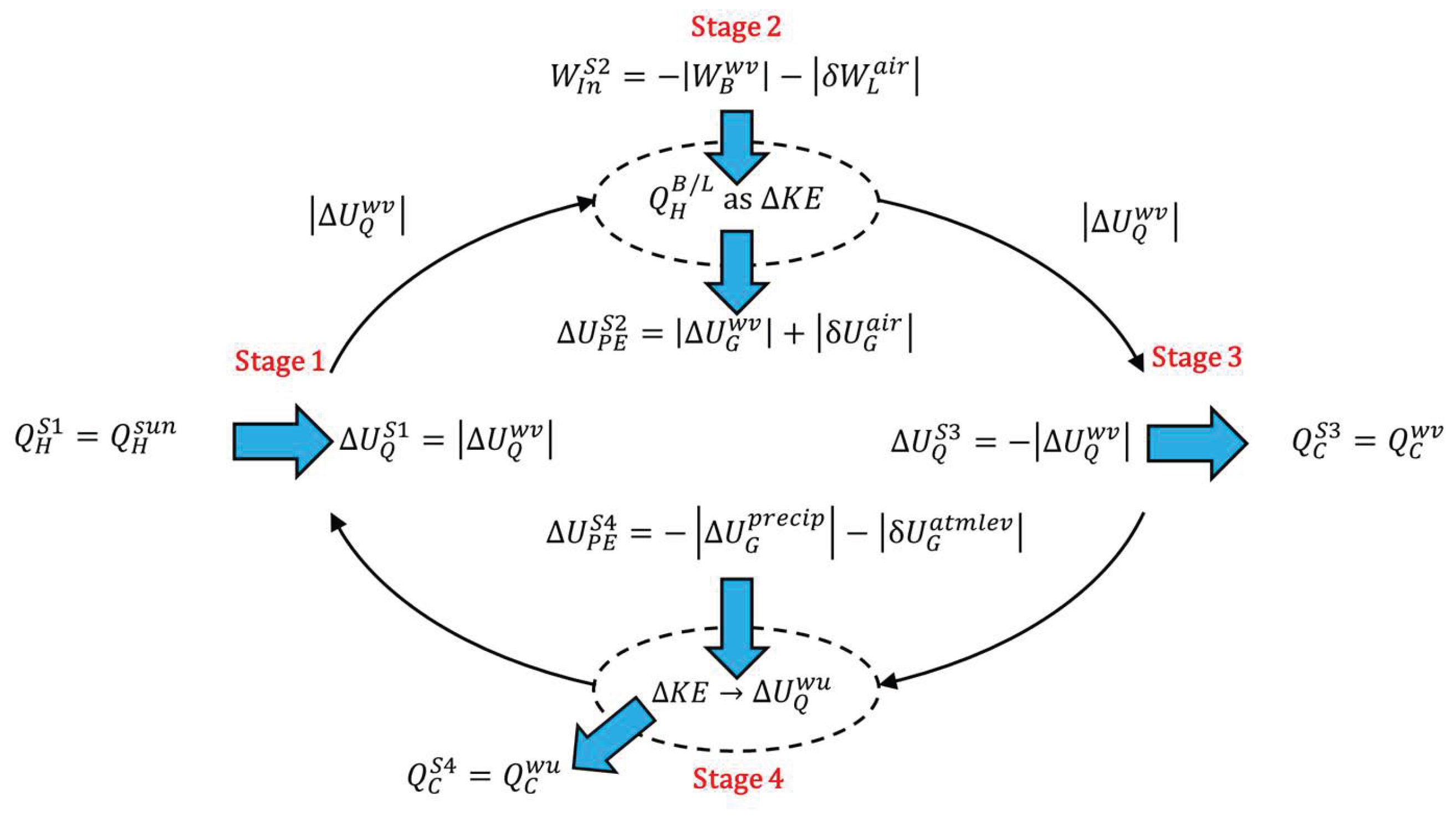
Appendix A.1. Analysis of Stages 1 Through 3 of the TWC
Start with applying the first law of thermodynamics and the work-energy theorem from Equation 11 to the system (subscript sys) for stages 1 through 3 (superscript ),
Total system energy change is the sum of state energy changes of internal energy of heat capacity and potential energy occurring during the stages. There are two changes in state property of internal energy of heat capacity (subscript Q) at stage 1 (superscript S1) and stage 3 (superscript S3) and one change in the state property of potential energy (subscript PE) at stage 2 (superscript S2),
The process property of net heat exchange of the system is the difference in heat input from the heat source (subscript H) at stage 1 and heat output to the heat sink (subscript C) ats stage 3 (superscript S3),
The process property of work output is the difference between work output and work input. Gravitational work is included in the state property of potential energy according to the work-energy theorem. There is no work output, but there is work input at stage 2,
Substitute Equation A2, Equation A3, and Equation A4 into Equation A1 to obtain the energy balance for stages 1 through 3 of the model (also Equation 13),
At stage 1, heat comes from the Sun (superscript sun),
heating and evaporating water, resulting in water vapor (superscript wv) with an increase in internal energy,
At stage 2, the buoyancy (subscript B) and lift (subscript L) of the atmosphere (superscript air) accelerate molecules into molecular-kinetic energy that is heat generated by both (superscript B/L),
Substitute Equation A6 and Equation A8 into Equation A5:
Rearrange right hand side of Equation A9,
revealing that the heat input (subscript in) for stages 1 through 3 is
and the heat output (subscript out) is
Displacement of water vapor and air becomes gravitational (subscript G) potential energy,
At stage 3, water condenses,
and loss of internal energy becomes heat output,
Substitute Equation A7, Equation A8, Equation A13, Equation A14, and Equation A15 into Equation A10,
To obtain the heat input and heat output for stages 1 through 3, substitute Equation A16 into Equation A11 (also Equation 21),
and substitute Equation A15 into Equation A12,
Appendix A.2. Analysis of Stage 4 of the TWC
To analyze stage 4 (superscript S4), apply the first law of thermodynamics and the work-energy theorem,
Total system energy change is due to one change in potential energy,
The net heat exchange is due to a heat output,
There is no work performed other than what is already included in the change in potential energy,
Substitute Equation A20, Equation A21, and Equation A22 into Equation A19 to obtain the energy balance (also Equation 16),
There is no heat input for stage 4,
There is a heat output for stage 4. The following analysis determines the quantity of this heat output,
At stage 4, water precipitates (superscript precip) and causes the atmosphere to level (superscript atmlev),
The gravitational potential energy that is gained at stage 2 is lost at stage 4:
Substitute Equation A26 and Equation A27 into Equation A23,
The released gravitational potential energy converts to bulk kinetic energy of water and air that completely thermalizes into molecular-kinetic energy, , and becomes internal energy of the water as it warms up (superscript wu),
The increase in internal energy dissipates into the environment from the water as warmup heat,
Substitute Equation A30 into Equation A28 for the energy balance to reveal that heat dissipated into the environment at stage 4 comes from release gravitational potential energy,
Substitute Equation A30 and Equation A31 into Equation A25 to determine heat output of stage 4 (also Equation 23),
Appendix A.3. Results of Heat Dissipations of Stages 1 through 4
The first result is revealed by comparing total heat input to total heat output. Sum Equation A17 and Equation A24 to determine the total heat input for stages 1 through 4:
Sum Equation A18 and Equation A32 to determine the total heat output for stages 1 through 4,
Compare Equation A24 and Equation A32,
to reveal that total heat input equals total heat output.
The second result is revealed by comparing the difference of heat input and heat output of stages 1 through 3 to the difference of heat input and heat output of stage 4. The difference for stages 1 through 3 is
This is the amount of energy that is stored during stage 2. The difference for stage 4 is
This is the amount of stored energy that is released at stage 4. The result is that the stored energy at stage 2 is equal and opposite to the released energy at stage 4,
This reveals that stage 2 and stage 4 of the TWC DS are reversible. The reversibility is a result of conservative forces controlling the storage and release of energy.
References
- Darwin, C. On the Origin of Species by Means of Natural Selection, Or, The Preservation of Favoured Races in the Struggle for Life; J. Murray: London, 1859. [Google Scholar]
- Carter, B. The Anthropic Principle and Its Implications for Biological Evolution. Philos. Trans. R. Soc. Lond. Ser. Math. Phys. Sci. 1983, 310, 347–363. [Google Scholar] [CrossRef]
- Barrow, J.D.; Tipler, F.J. The Anthropic Cosmological Principle; Oxford University Press, 1986; ISBN 978-0-19-851949-2. [Google Scholar]
- Hanson, R. Must Early Life Be Easy? The Rhythm of Major Evolutionary Transitions. 1998. Available online: https://mason.gmu.edu/~rhanson/hardstep.pdf.
- Watson, A.J. Implications of an Anthropic Model of Evolution for Emergence of Complex Life and Intelligence. Astrobiology 2008, 8, 175–185. [Google Scholar] [CrossRef] [PubMed]
- McKay, C.P. Time For Intelligence On Other Planets; 1 January 1996; p. 405. [Google Scholar]
- Carter, B. Five- or Six-Step Scenario for Evolution? Int. J. Astrobiol. 2008, 7, 177–182. [Google Scholar] [CrossRef]
- McCabe, M.; Lucas, H. On the Origin and Evolution of Life in the Galaxy. Int. J. Astrobiol. 2010, 9, 217–226. [Google Scholar] [CrossRef]
- Lenton, T.; Watson, A. Revolutions That Made the Earth; Oxford University Press, 2011; ISBN 978-0-19-958704-9. [Google Scholar]
- Lingam, M.; Loeb, A. Role of Stellar Physics in Regulating the Critical Steps for Life. Int. J. Astrobiol. 2019, 18, 527–546. [Google Scholar] [CrossRef]
- The Timing of Evolutionary Transitions Suggests Intelligent Life Is Rare | Astrobiology. Available online: https://www.liebertpub.com/doi/10.1089/ast.2019.2149 (accessed on 31 January 2026).
- Mills, D.B.; Macalady, J.L.; Frank, A.; Wright, J.T. A Reassessment of the “Hard-Steps” Model for the Evolution of Intelligent Life. Sci. Adv. 2025, 11. [Google Scholar] [CrossRef] [PubMed]
- Spiegel, D.S.; Turner, E.L. Bayesian Analysis of the Astrobiological Implications of Life’s Early Emergence on Earth. Proc. Natl. Acad. Sci. 2012, 109, 395–400. [Google Scholar] [CrossRef] [PubMed]
- Flambaum, V.V. Comment on “Does the Rapid Appearance of Life on Earth Suggest That Life Is Common in the Universe?”. Astrobiology 2003, 3, 237–239. [Google Scholar] [CrossRef]
- Wright, J.T.; Kanodia, S.; Lubar, E. How Much SETI Has Been Done? Finding Needles in the n-Dimensional Cosmic Haystack. Astron. J. 2018, 156, 260. [Google Scholar] [CrossRef]
- Livio, M. How Rare Are Extraterrestrial Civilizations, and When Did They Emerge? Astrophys. J. 1999, 511, 429. [Google Scholar] [CrossRef]
- Crawford, I.A.; Schulze-Makuch, D. Is the Apparent Absence of Extraterrestrial Technological Civilizations down to the Zoo Hypothesis or Nothing? Nat. Astron. 2024, 8, 44–49. [Google Scholar] [CrossRef]
- Star Masses and Star-Planet Distances for Earth-like Habitability | Astrobiology. Available online: https://www.liebertpub.com/doi/10.1089/ast.2016.1518 (accessed on 31 January 2026).
- Weiss, M.C.; Sousa, F.L.; Mrnjavac, N.; Neukirchen, S.; Roettger, M.; Nelson-Sathi, S.; Martin, W.F. The Physiology and Habitat of the Last Universal Common Ancestor. Nat. Microbiol. 2016, 1, 16116. [Google Scholar] [CrossRef] [PubMed]
- Moody, E.R.R.; Álvarez-Carretero, S.; Mahendrarajah, T.A.; Clark, J.W.; Betts, H.C.; Dombrowski, N.; Szánthó, L.L.; Boyle, R.A.; Daines, S.; Chen, X.; et al. The Nature of the Last Universal Common Ancestor and Its Impact on the Early Earth System. Nat. Ecol. Evol. 2024, 8, 1654–1666. [Google Scholar] [CrossRef]
- Erwin, D.H. The End and the Beginning: Recoveries from Mass Extinctions. Trends Ecol. Evol. 1998, 13, 344–349. [Google Scholar] [CrossRef]
- Bond, D.P.G.; Grasby, S.E. On the Causes of Mass Extinctions. Palaeogeogr. Palaeoclimatol. Palaeoecol. 2017, 478, 3–29. [Google Scholar] [CrossRef]
- Elewa, A.M.T.; Abdelhady, A.A. Past, Present, and Future Mass Extinctions. J. Afr. Earth Sci. 2020, 162, 103678. [Google Scholar] [CrossRef]
- Halliday, A.N.; Canup, R.M. The Accretion of Planet Earth. Nat. Rev. Earth Environ. 2023, 4, 19–35. [Google Scholar] [CrossRef]
- Kirkland, C.L.; Johnson, T.E.; Brown, M.; Smithies, H.; Drabon, N.; O’Neill, C. The Evolution of Earth’s Early Continental Crust. Nat. Rev. Earth Environ. 2025, 6, 612–625. [Google Scholar] [CrossRef]
- Glavin, D.P.; Dworkin, J.P.; Alexander, C.M.O.; Aponte, J.C.; Baczynski, A.A.; Barnes, J.J.; Bechtel, H.A.; Berger, E.L.; Burton, A.S.; Caselli, P.; et al. Abundant Ammonia and Nitrogen-Rich Soluble Organic Matter in Samples from Asteroid (101955) Bennu. Nat. Astron. 2025, 9, 199–210. [Google Scholar] [CrossRef] [PubMed]
- McCoy, T.J.; Russell, S.S.; Zega, T.J.; Thomas-Keprta, K.L.; Singerling, S.A.; Brenker, F.E.; Timms, N.E.; Rickard, W.D.A.; Barnes, J.J.; Libourel, G.; et al. An Evaporite Sequence from Ancient Brine Recorded in Bennu Samples. Nature 2025, 637, 1072–1077. [Google Scholar] [CrossRef]
- Burkhart, B.; Dharmawardena, T.E.; Bialy, S.; Haworth, T.J.; Cruz Aguirre, F.; Jo, Y.-S.; Andersson, B.-G.; Chung, H.; Edelstein, J.; Grenier, I.; et al. A Nearby Dark Molecular Cloud in the Local Bubble Revealed via H2 Fluorescence. Nat. Astron. 2025, 9, 1064–1072. [Google Scholar] [CrossRef] [PubMed]
- Rousseau, P.; Piekarski, D.G.; Capron, M.; Domaracka, A.; Adoui, L.; Martín, F.; Alcamí, M.; Díaz-Tendero, S.; Huber, B.A. Polypeptide Formation in Clusters of β-Alanine Amino Acids by Single Ion Impact. Nat. Commun. 2020, 11, 3818. [Google Scholar] [CrossRef] [PubMed]
- Griffith, E.C.; Vaida, V. In Situ Observation of Peptide Bond Formation at the Water–Air Interface. Proc. Natl. Acad. Sci. 2012, 109, 15697–15701. [Google Scholar] [CrossRef]
- Joule, J.P., III. On the Mechanical Equivalent of Heat. Philos. Trans. R. Soc. Lond. 1850, 61–82. [Google Scholar] [CrossRef]
- Young, J. Heat, Work and Subtle Fluids: A Commentary on Joule (1850) ‘On the Mechanical Equivalent of Heat. Philos. Transact. A Math. Phys. Eng. Sci. 2015, 373, 20140348. [Google Scholar] [CrossRef]
- Clausius, R. Ueber Die Bewegende Kraft Der Wärme Und Die Gesetze, Welche Sich Daraus Für Die Wärmelehre Selbst Ableiten Lassen. Ann. Phys. 1850, 155, 500–524. [Google Scholar] [CrossRef]
- Clausius, R. I. On the Moving Force of Heat, and the Laws Regarding the Nature of Heat Itself Which Are Deducible Therefrom. Lond. Edinb. Dublin Philos. Mag. J. Sci. 1851, 2, 1–119. [Google Scholar] [CrossRef]
- Maxwell, J.C., II. Illustrations of the Dynamical Theory of Gases. Lond. Edinb. Dublin Philos. Mag. J. Sci. 1860, 20, 21–37. [Google Scholar] [CrossRef]
- Garber, E.W. Clausius and Maxwell’s Kinetic Theory of Gases. Hist. Stud. Phys. Sci. 1970, 2, 299–319. [Google Scholar] [CrossRef]
- Clausius, R. I. Ueber verschiedene für die Anwendung bequeme Formen der Hauptgleichungen der mechanischen Wärmetheorie. Ann. Phys. Chem. 1865, 125, 353–400. [Google Scholar] [CrossRef]
- Clausius, R. The Mechanical Theory of Heat: With Its Applications to the Steam-Engine and to the Physical Properties of Bodies; J. Van Voorst: London, 1867; Available online: https://books.google.com/books/about/The_Mechanical_Theory_of_Heat.html?id=8LIEAAAAYAAJ.
- Clausius, R. The Mechanical Theory of Heat; Macmillan and Co.: London, 1879; Available online: https://www.google.com/books/edition/The_Mechanical_Theory_of_Heat/7MCmNuSl9zYC.
- Pérez-García, C.; Echebarria, B. Bénard Cells: A Centennial Puzzle. In Instabilities and Nonequilibrium Structures VI; Tirapegui, E., Martínez, J., Tiemann, R., Eds.; Springer Netherlands: Dordrecht, 2000; pp. 165–176. ISBN 978-94-011-4247-2. [Google Scholar]
- Prigogine, I.; Wiame, J.M. Biologie et thermodynamique des phénomènes irréversibles. Experientia 1946, 2, 451–453. [Google Scholar] [CrossRef]
- Prigogine, I.; Nicolis, G. Biological Order, Structure and Instabilities. Q. Rev. Biophys. 1971, 4, 107–148. [Google Scholar] [CrossRef]
- Nicolis, G.; Prigogine, I. Self-Organization in Nonequilibrium Systems: From DSs to Order through Fluctuations; Wiley: New York, 1977; ISBN 978-0-471-02401-9. [Google Scholar]
- Prigogine, I.; Nicolis, G. Self-Organisation in Nonequilibrium Systems: Towards A Dynamics of Complexity. In Bifurcation Analysis: Principles, Applications and Synthesis; Hazewinkel, M., Jurkovich, R., Paelinck, J.H.P., Eds.; Springer Netherlands: Dordrecht, 1985; pp. 3–12. ISBN 978-94-009-6239-2. [Google Scholar]
- Irons, L.G.; Irons, M.A. Pancosmorio (World Limit) Theory of the Sustainability of Human Migration and Settlement in Space. Front. Astron. Space Sci. 2023, 10. [Google Scholar] [CrossRef]
- Sands, D. The Carnot Cycle, Reversibility and Entropy. Entropy 2021, 23, 810. [Google Scholar] [CrossRef]
- Toyabe, S.; Sagawa, T.; Ueda, M.; Muneyuki, E.; Sano, M. Experimental Demonstration of Information-to-Energy Conversion and Validation of the Generalized Jarzynski Equality. Nat. Phys. 2010, 6, 988–992. [Google Scholar] [CrossRef]
- Martyushev, L.M.; Seleznev, V.D. Maximum Entropy Production Principle in Physics, Chemistry and Biology. Phys. Rep. 2006, 426, 1–45. [Google Scholar] [CrossRef]
- Martyushev, L.M. The Maximum Entropy Production Principle: Two Basic Questions. Philos. Trans. R. Soc. B Biol. Sci. 2010, 365, 1333–1334. [Google Scholar] [CrossRef]
- Kleidon, A.; Fraedrich, K.; Kunz, T.; Lunkeit, F. The Atmospheric Circulation and States of Maximum Entropy Production. Geophys. Res. Lett. 2003, 30. [Google Scholar] [CrossRef]
- Kleidon, A.; Malhi, Y.; Cox, P.M. Maximum Entropy Production in Environmental and Ecological Systems. Philos. Trans. R. Soc. B Biol. Sci. 2010, 365, 1297–1302. [Google Scholar] [CrossRef] [PubMed]
- Kleidon, A. Non-Equilibrium Thermodynamics, Maximum Entropy Production and Earth-System Evolution. Philos. Trans. R. Soc. Math. Phys. Eng. Sci. 2010, 368, 181–196. [Google Scholar] [CrossRef]
- Jørgensen, S.E. Introduction to Systems Ecology; CRC Press: Boca Raton, 2016; ISBN 978-0-429-10775-7. [Google Scholar]
- Kiehl, J.T.; Trenberth, K.E. Earth’s Annual Global Mean Energy Budget. Bull. Am. Meteorol. Soc. 1997, 78, 197–208. [Google Scholar] [CrossRef]
- Trenberth, K.E.; Fasullo, J.T.; Kiehl, J. Earth’s Global Energy Budget. Bull. Am. Meteorol. Soc. 2009, 90, 311–324. [Google Scholar] [CrossRef]
- Loeb, N.G.; Wielicki, B.A.; Doelling, D.R.; Smith, G.L.; Keyes, D.F.; Kato, S.; Manalo-Smith, N.; Wong, T. Toward Optimal Closure of the Earth’s Top-of-Atmosphere Radiation Budget. J. Clim. 2009, 22, 748–766. [Google Scholar] [CrossRef]
- Sharp, K.; Matschinsky, F. Translation of Ludwig Boltzmann’s Paper “On the Relationship between the Second Fundamental Theorem of the Mechanical Theory of Heat and Probability Calculations Regarding the Conditions for Thermal Equilibrium” Sitzungberichte Der Kaiserlichen Akademie Der Wissenschaften. Mathematisch-Naturwissen Classe. Abt. II, LXXVI 1877, Pp 373-435 (Wien. Ber. 1877, 76:373-435). Reprinted in Wiss. Abhandlungen, Vol. II, Reprint 42, p. 164-223, Barth, Leipzig, 1909. Entropy 015, 17, 1971–2009. [Google Scholar] [CrossRef]
- Irons, L.G. Pre-Biotic Earth and a More Complete Theory of Heat Transfor-Mation, Part II. Entropy 2026, TBD. [Google Scholar]
- Schrödinger, E. What Is Life? The Macmillan Company: Cambridge, 1945; Available online: http://archive.org/details/whatislife0000erwi.
| 1 | Laying aside any current debates regarding what the universe is and whether it is an isolated system or an open system, we can say that the observable universe with its hot spots of stars and other celestial objects collected in clusters of galaxies spread in a web of mass filaments within a cosmic microwave background radiation (CMBR) of 2.7 K does not appear to have changed temperature much at all over the course of the history of existence of Earth. For the purposes of this paper, that “limited” time period of Earth history is sufficient to say that the universe approximates an ideal system in thermal equilibrium relative to the open system of Earth. |
| 2 | An example of a real system that can be modeled as convective heat transfer in an open system simple-heat-transfer model is a Bénard cell [40]. A Barnard cell is an example of a DS that does not involve a conservative force field. DSs that utilize conservative force fields are discussed further down in this article. |
| 3 | Textbooks and literature commonly symbolize both internal energy and potential energy using the term ∆U, so the subscripts of Q, PE, and G are used to differentiate between the internal energy of heat capacity and the potential energy of gravity. What they have in common beyond the symbol is that they are both forms of stored, captured, or contained energy. |
| 4 | Liquid water and even frozen water can result. Considering that some of the original evaporation/sublimation into water vapor comes from regions of snow and ice, effects of such subcooling into cold water and ice/snow are considered to be averaged out of this model. |
| 5 | Universal entropy is generated by the warmup heat expelled at stage 4, but buoyancy’s fundamental conservative quality is not reduced. This reveals that gravity wells are endless sources of additional energy when heat from other sources dissipates through them. This is a seeming paradox to the definition of entropy in that universal entropy from released gravitational potential energy does not deplete the source of gravity. While there is mass available to form gravity wells and while there is heat of any quality available to fall into gravity wells, GDSs would seem to continue to exist. The presence of life within this enigma is an interesting correlation. |
| 6 | In the discussion of APC and ARO for GDSs, the calculations presented are based on present-day empirically determined solar insolation and Earth budget values. The calculated APC and ARO are maximum steady state values. These calculations are provided as examples. Knowing the level of solar insolation for a pre-biotic Earth would enable similar calculations. The same equations would apply, consdiering the the physics of gravity and heat transfer is the same for pre-biotic Earth as it is for contemporary Earth. |
| 7 | The total additional gravidynamics power flux introduced to Earth is 252 Watts per square meter, which is greater than the estimate of 95 Watts per square meter estimated in [45], which results in the sum of the inputs to Earth by the solar power with the related gravidynamic response to solar power being 491 Watts per square meter. This is greater than the 334 Watts per square meter estimated [45]. |
| 8 | The temperature inversion in the stratosphere is a result of the chemical reaction driven by solar radiation that generates Oxygen-3 (ozone). The ozone chemical reaction is stage 2 of a chemical DS. Chemical DSs are discussed below. |
| 9 | The poetic and literal meaning of “burns out” is that the heat is still one or more steps away from dissipating into the universal heat sink when the specific heat quality output is so low that the only thing the heat can do is dissipate into the average local internal energy of the Earth environment, its last use being to maintain average temperatures on Earth. It becomes a foundation for local heat temperatures of all the DSs in the network that the heat passed through to get to this point, similar to the heat generated in the Earth core, mantel, and crust that is left over from the initial formation of Earth, the heat that is generated by gravitational interaction of Earth with the Sun and Moon, the heat that is generated by friction of the spin of Earth, and the heat of augmentational activity generated by humans and other tool-using animals on Earth. This is effectively the ultimate, last DS with the complexity yield comprised of the storage of internal energy of Earth in the form of the heat capacities of the materials of Earth, and the final ARO, specific heat quality drop, and local heat output at stage 4 being the black-body radiation of Earth. |
Figure 1.
A model of an open system (subscript sys) with a heat source (subscript H) from which and a heat sink (subscript C) to which the open system undergoes a simple heat transfer process. The following variables are used: – heat transfer rate into and out of the system, – heat transfer coefficient of matter in system, – cross-sectional area of system of matter, – length of system of matter from heat source to heat sink, – mass flow rate, – specific heat capacity at constant pressure (subscript p) , – temperature of the heat source, – temperature of the heat sink, – average (subscript avg) temperature of the system, – the rate of change of internal energy of the system.
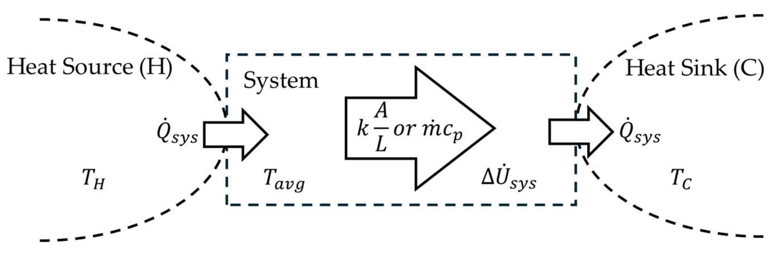
Figure 2.
A model of an open system with a heat source from which and a heat sink to which the open system undergoes a heat transfer process in the presence of a conservative force field. The following new variables are introduced: – heat leaving the heat source and entering the system, – heat leaving the system and entering the heat sink, – work input to the system, – internal energy of heat capacity of the system, – potential energy of the system associated with the conservative force field. The total energy contained by the system is .
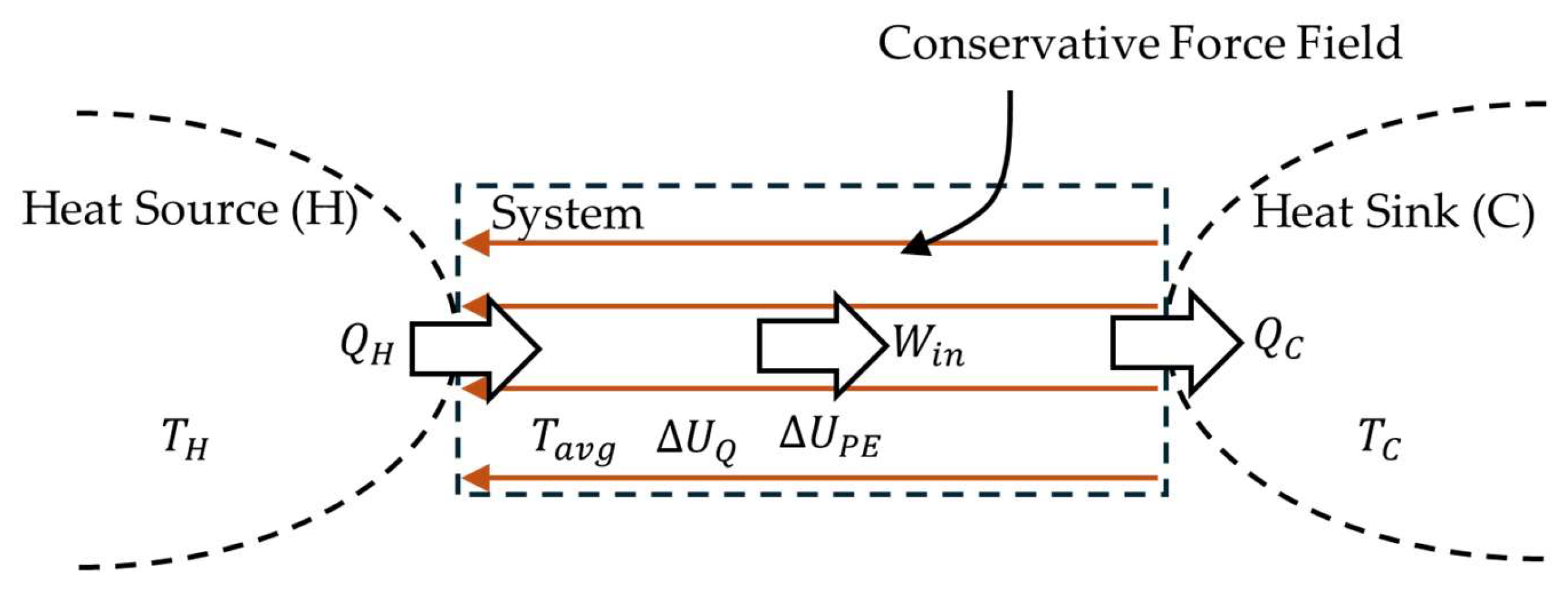
Figure 3.
The potential energy function of a point source potential energy well. The potential energy is proportional to the negative inverse of the distance from the point source of a conservative force field.
Figure 3.
The potential energy function of a point source potential energy well. The potential energy is proportional to the negative inverse of the distance from the point source of a conservative force field.
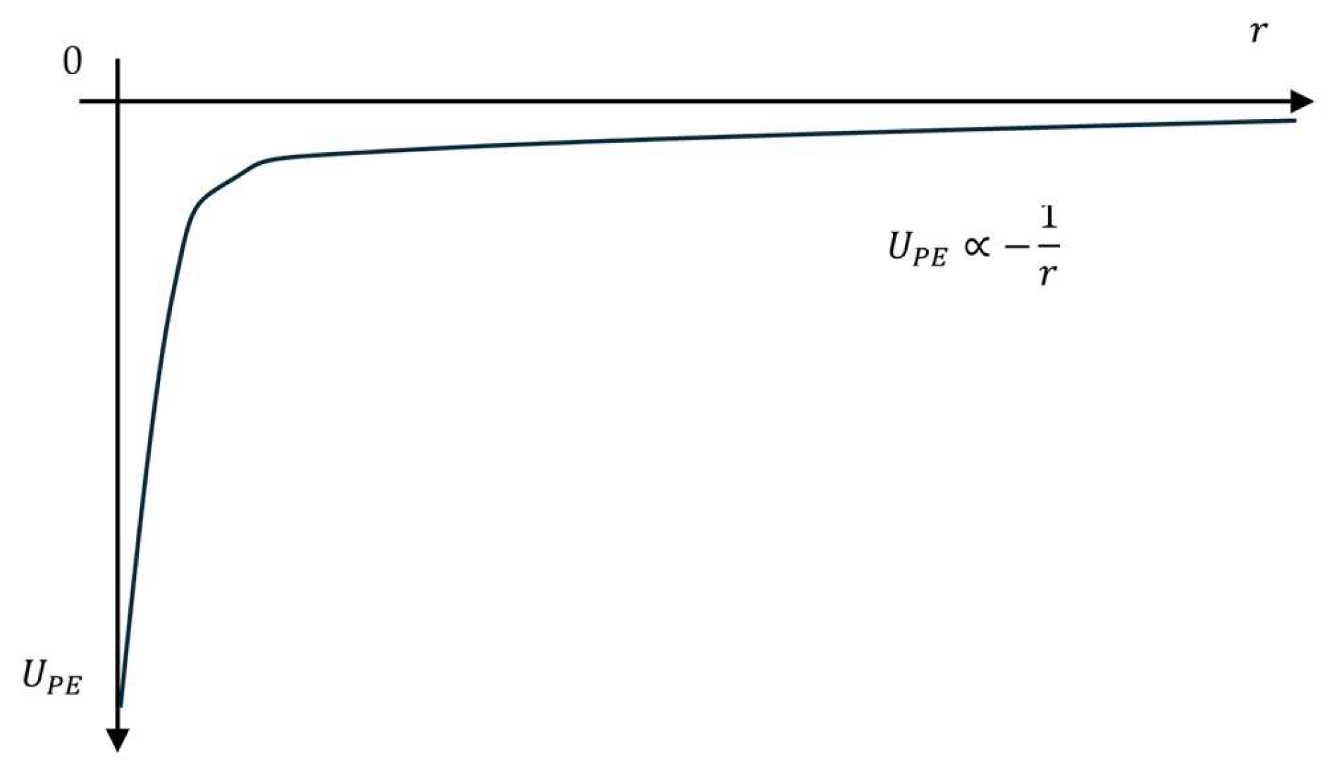
Figure 4.
The tropospheric water cycle (TWC). At stage 1 (S1), liquid water absorbs the heat of solar radiation, , and evaporates into gaseous form. At stage 2 (S2), the buoyant force, , performs work on the water vapor, , by lifting the water vapor to higher altitudes, . As this occurs, the force of gravity, , acts against the lift, resulting in an increase in potential energy of the water vapor, . At stage 3 (S3), the heat released by condensing water vapor, , dissipates into the upper atmosphere and space. At stage 4 (S4), the water falls back to Earth’s surface as precipitation and flows to the lowest point in Earth’s gravitational well that it can reach, returning to the beginning of stage 1 where it can again absorb solar radiation.
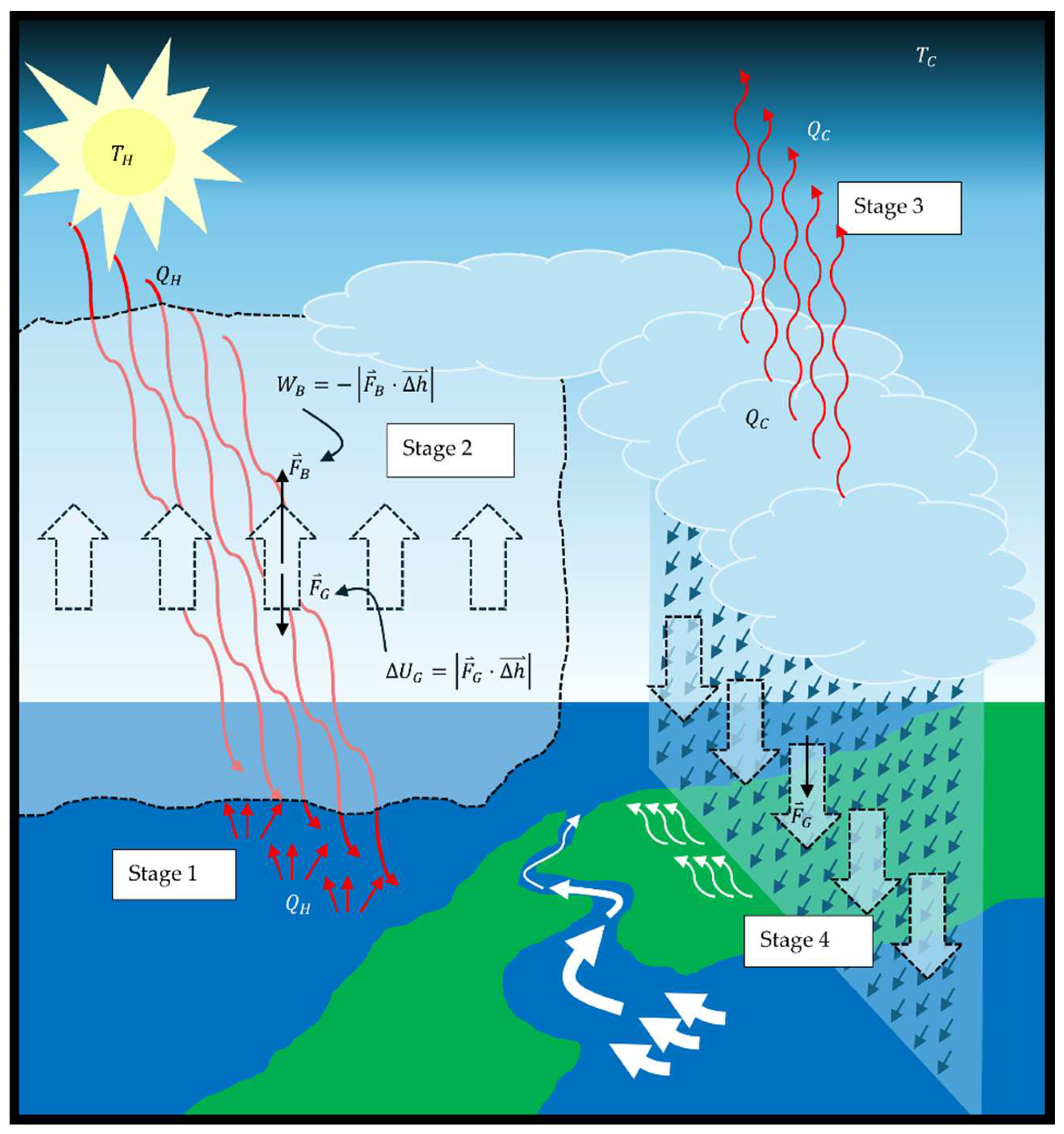
Figure 5.
Atmospheric lift results from the expansion of water vapor that displaces dry air to higher altitudes. When the sun sets and the night side of Earth loses solar insolation, the water vapor remaining in the air contracts, resulting the atmosphere compressing to lower altitudes. Air pressure at altitude adjusts conservatively based upon the weight of the air column under the influence of gravity (determined the density and depth in the atmosphere). This causes the atmosphere to act like a conservative piston, considering the force of gravity is not depleted by the lift and subsequent leveling.
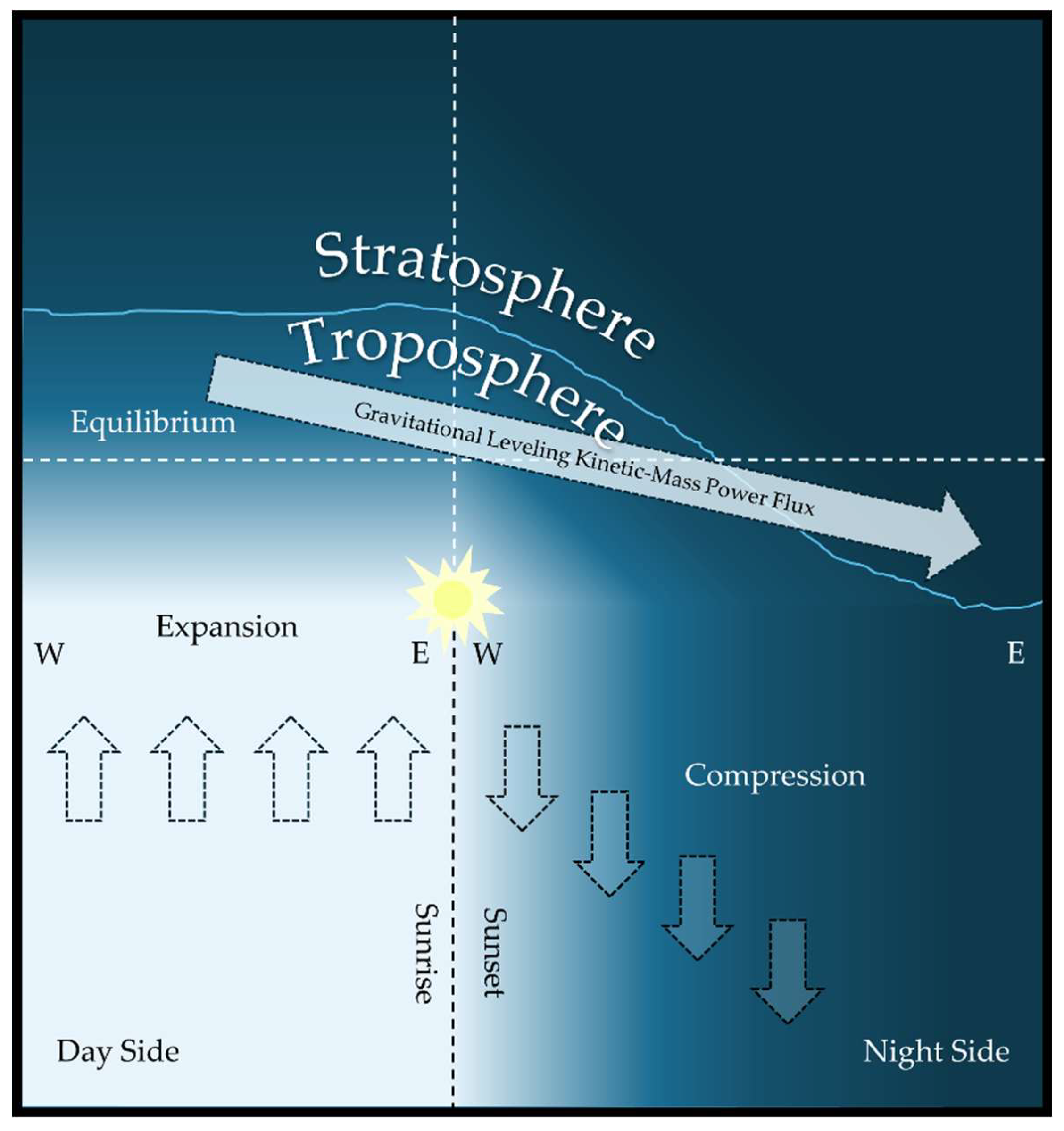
Figure 6.
Buoyancy driven by atmospheric depth pressure performs work on water vapor and air. The work is converted to molecular-kinetic energy, effectively acting as a source of heat input. The molecular-kinetic energy of work-heat is then converted into gravitational potential energy. Any water that condenses and falls at any time during the entire cycle is returned to ground level because of the conservative nature of the force of gravity. The work of buoyancy that is stored as gravitational potential energy converts back to molecular-kinetic energy as the water molecules are accelerated by gravity. This injects into the Earth system an amount of internal energy of heat capacity equivalent to the energy of the work performed by the buoyant force in previously lifting the water to higher altitudes in the atmosphere. The injected internal energy is then free to dissipate as heat into the environment.
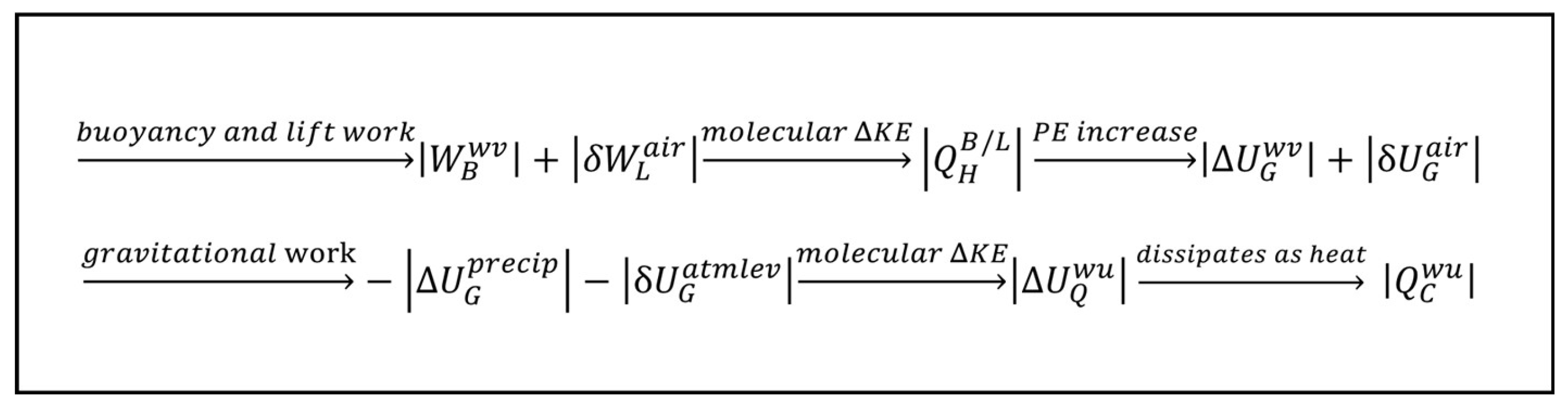
Figure 7.
Heat input from the universal heat source to the local heat source is equal to heat output from the local heat source to the DS. The contributions of these two heat transfers to the change in non-equilibrium entropy of the local heat source are equal and opposite, resulting in the change in local heat source non-equilibrium entropy being zero. The same argument applies to the local heat sink.
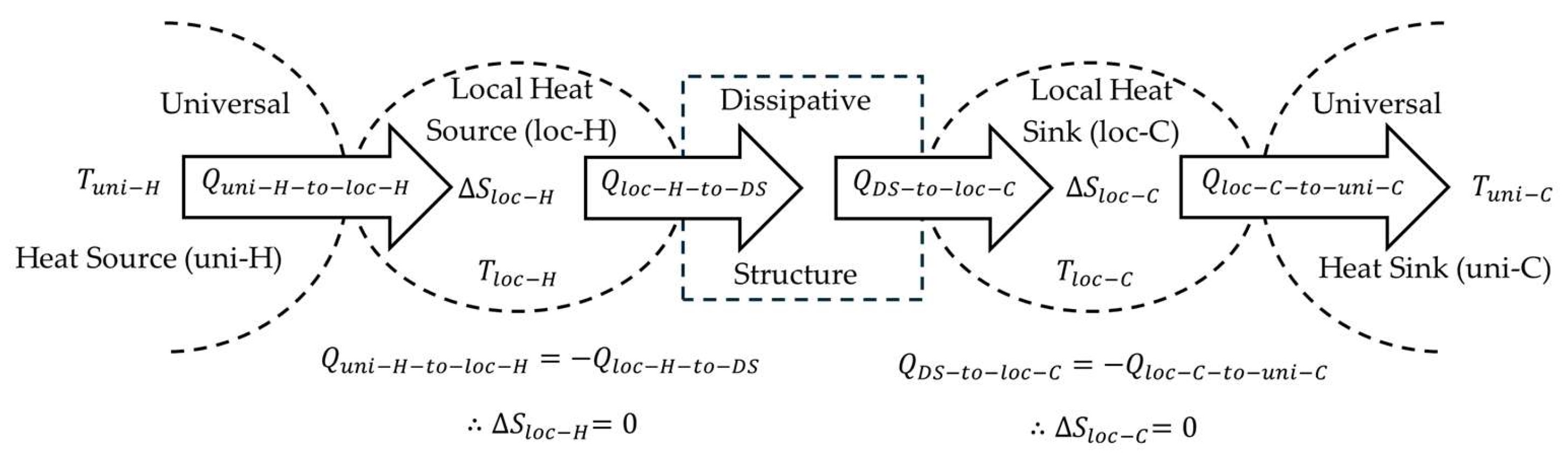
Disclaimer/Publisher’s Note: The statements, opinions and data contained in all publications are solely those of the individual author(s) and contributor(s) and not of MDPI and/or the editor(s). MDPI and/or the editor(s) disclaim responsibility for any injury to people or property resulting from any ideas, methods, instructions or products referred to in the content. |
© 2026 by the author. Licensee MDPI, Basel, Switzerland. This article is an open access article distributed under the terms and conditions of the Creative Commons Attribution (CC BY) license (http://creativecommons.org/licenses/by/4.0/).
Copyright: This open access article is published under a Creative Commons CC BY 4.0 license, which permit the free download, distribution, and reuse, provided that the author and preprint are cited in any reuse.


