
Submitted:
20 February 2026
Posted:
26 February 2026
You are already at the latest version
Abstract
Early detection is a key tool for preventing wildfires. Modern machine learning algorithms integrated into large-scale monitoring systems enable automated surveillance of high-risk areas. However, single‑image detection methods that do not consider interframe dependencies and changes between consecutive images often fail to detect smoke plumes at the very early stage and at larger distances, critical for effective response, or they produce an increased number of false alarms. Biological vision is particularly sensitive to motion cues, and this translates well to automated systems. Recent temporal-memory approaches have demonstrated improved performance over purely spatial methods but typically rely on complex, computationally heavy multi-stage architectures.
This study investigates the possibility of encoding temporal and contextual information into additional image channels as a basis for compiling data models with increased information content. Several distinct data models were proposed, and corresponding datasets were generated to train standard YOLO architectures. Experimental evaluation compared the performance of YOLO models trained on the information‑enriched datasets with those trained on standard RGB images. Based on the results, the best data model for early wildfire smoke detection was selected. Comparative evaluation demonstrated improved detection accuracy for models trained on data containing spatio-temporal information compared to standard RGB images, while preserving low inference latency. The proposed approach shifts the focus to the structure and information content of the data while preserving the efficiency of standard convolutional neural network architectures. This approach could be applied to other problems requiring high efficiency and real-time operation, where temporal and contextual information can improve detection performance.
Keywords:
data models
; smoke detection
; wildfire surveillance
; YOLO
; machine learning
1. Introduction
Wildfires are among the most destructive natural phenomena, significantly affecting human lives and entire ecosystems. The consequences of large wildfires are not only short-term and often catastrophic but also cause lasting changes to communities and leave impacts on the ecosystem that can be visible for decades. Early and accurate detection is therefore paramount in mitigating the devastating effects of wildfires, enabling a more rapid response and containment before they escalate into uncontrollable conflagrations [1,2]. Technological advances and the development of advanced image-processing algorithms have enabled a shift from systems relying on trained human observers to technological solutions based on surveillance cameras and automatic detection algorithms [3,4,5]. Although these systems have improved wildfire monitoring, the complex nature of smoke, which is the first visible sign of wildfire during daytime, often results in many false alarms as well as missed detections. The semi-transparent nature of smoke, the lack of clearly defined features, image quality degradation due to atmospheric and other disturbances, and the need to detect fires at long distances and at the earliest stages make early wildfire smoke detection extremely challenging [6]. This challenge is compounded by the varying shapes, sizes, and colors of smoke plumes, alongside potential sensor degradation, which collectively hinder effective spatial information extraction from a single image.The rapid development of deep learning and convolutional neural networks has greatly enhanced image analysis and computer vision capabilities. These algorithms have found applications across many domains, including early smoke detection for wildfires [1,7,8]. Specifically, You Only Look Once (YOLO) architectures [9] have emerged as particularly promising due to their real-time performance and high accuracy in object detection tasks, even in complex environmental conditions [10,11]. However, the inherent limitations of processing static RGB images for dynamic phenomena like smoke propagation still present significant hurdles for these models, often leading to reduced precision and increased false positive rates in real-world scenarios [12].
The pronounced sensitivity of human vision to motion and change has inspired approaches that combine temporal information from sequences of consecutive frames with the spatial information contained in a single image, aiming to improve detection accuracy. These methods often relay on hybrid multi-stage algorithms that combine different neural network architectures to extract spatial and temporal information [13,14,15]. While effective, such complex neural network architectures can be computationally intensive, which may be limiting factor for large-scale deployment, where the system is expected to infer multiple high-resolution streams at the same time, necessitating alternative strategies to integrate temporal cues with spatial features without significantly increasing model complexity or inference times [16,17,18].
In order to circumvent these limitations while still providing the benefits of temporal information cues, this study investigates the possibility of increasing the information content of the data by adding temporal and contextual information into additional image channels, instead of customizing neural networks for video stream processing. This work builds upon our prior research that explores the integration of diverse data models for enhanced smoke detection [19]. The proposed strategy reduces computational overhead by directly integrating spatio-temporal data into a unified input format for streamlined processing by existing, highly optimized object detection models.
This study is based on a dataset collected from the archive of intelligent wildfire surveillance system currently operational at 116 locations in the Republic of Croatia, as well as at additional sites in Bosnia and Herzegovina, Montenegro, and Albania [20]. The surveillance locations in Croatia are shown in Figure 1. This archive contains recordings collected under various atmospheric and visibility conditions, with image-quality degradation that occurs during use of surveillance cameras at remote and isolated locations throughout the year. The archive contains footage of real forest fires in the earliest stages and at different distances from the camera.
Sequences of images with duration of 30 to 45 minutes were retrieved from the system archive. By processing consecutive frames, additional image channels encoding temporal and contextual information were generated. These supplementary channels were combined with the existing RGB channels to form multidimensional samples that capture spatial, temporal, and contextual information. By combining these additional features extracted from sequences of consecutive frames, six multidimensional data models with different combinations of spatial, temporal, and contextual information were compiled, and a separate dataset was generated for each data model. These multichannel datasets were used to train a standard YOLO architecture, aiming to select the best data model for wildfire detection. The obtained results were compared with those achieved by training the same YOLO architecture in the same set of images using only RGB channels (standard image).
The evaluation methodology follows a three-stage evaluation process: (a) different models of multichannel data were evaluated on a limited-size data in order to select the best data model for wildfire smoke detection; (b) the best performing data model was retrained and evaluated on large dataset obtained using augmentation techniques, and (c) final validation was performed on the original high-resolution image sequences collected from a separate set of monitoring locations that were not used in earlier phases of the study. In this last evaluation step, a production wildfire surveillance environment was simulated to assess both the effectiveness of the proposed solution and its efficiency with respect to potential real-time deployment.
The main contribution of this work include: (a) the proposed approach of encoding temporal and contextual information in additional image channels, enabling the use of standard and efficient DNN architectures for processing video sequences; (b) selection of the optimal data model for wildfire smoke detection; (c) real-time smoke detection algorithm applicable to high-resolution video sequences; (d) a sequence augmentation technique that preserves the relationships between consecutive frames was proposed and (e) a wildfire smoke dataset was created containing original RGB images and additional spatio-temporal data and made available for future research.
The remainder of the paper is structured as follows. Section 2 provides an overview of existing research on smoke detection for early wildfire detection, and reviews deep learning methods that incorporate temporal information, with an emphasis on the YOLO algorithm. Section 3 details the methodology of the presented study, including the generation of multichannel data models and the evaluation procedure of the proposed approach. Section 4 presents the experimental results, followed by the conclusions in Section 5.
2. Related Work
The evolution of wildfire detection systems, from manual human observers to automated systems, has been primarily driven by computational capability and algorithmic complexity. While early automation approaches, such as histogram based algorithms [6], provided reasonable results, they required substantial post-processing and fine-tuning. More recently, rapid advances in GPU compute power enabled deep neural networks (DNN), particularly Convolutional Neural Networks (CNN) to become the dominant paradigm in computer vision based object detection [1,9,21].
Current industry standard for CNN-based real-time detection and segmentation tasks is the YOLO family of models, first introduced in 2016 [9]. By replacing the traditional multi-stage localization and detection approach of regular CNN networks with single-pass inference (with convolutional layers predicting both bounding boxes and class probabilities) YOLO achieved balance between accuracy and computational efficiency necessary for embedded hardware deployment. Each new version added architectural improvements and task-specific optimizations [22,23,24]. Due to their excellent real-time performance, YOLO models were quickly adopted into the sphere of wildfire detection [1,11,21,25].
Considering the practical constraints of deploying automated systems in remote locations, recent research focuses on lightweight CNN architectures capable of real-time smoke detection on resource limited hardware. El-Madafri et al. [26] propose a compact convolutional model optimized for lookout towers with CPU limited inference capabilities. Through hierarchical knowledge distillation accross multiple models, they reduce complexity while preserving accuracy. Their system processes single RGB frames from fixed cameras and achieves near real-time performance with competitive detection results, demonstrating that carefully designed lightweight CNNs can be deployed on edge devices for operational wildfire monitoring.
More recently, attention mechanisms have become popular with detection architectures to improve contextual understanding. For example, in [27] a swin transformer backbone is integrated into an optimized Faster R-CNN framework to improve feature extraction in complex outdoor scenes. The transformer’s superior context modeling capabilities improve discrimination between actual wildfire and benign events, yielding better results than CNN-only approaches. Unfortunately, the introduction of the transformer to the backbone comes at the cost of reduced inference speed.
This trade-off between performance and speed also comes to light with the latest YOLOv12 model architecture. While attention mechanics help YOLOv12 achieve better results compared to older models [24], specialized task-specific modifications often prove more effective for smoke detection, as demonstrated in recent studies [28,29,30]. For example, in F3-YOLO presented in [29], improvements to feature fusion in deeper CNN layers can surpass attention-based models like YOLOv12 while maintaining computational efficiency of pure CNN architectures.
Despite these architectural advances, for what concerns early smoke detection systems a fundamental limitation remains: they rely on individual frames without incorporating temporal motion data. Models trained on static RGB or thermal images inherently ignore the characteristic motion of smoke plumes. Their shape and speed varies, but at longer distances where spatial resolution degrades, the temporal motion of smoke becomes crucial discriminative information.
In line with this reasoning, recent studies increasingly use temporal information to boost wildfire smoke detection performance. The SmokeyNet model featured in [15] combines both a CNN backbone to extract the regions of interest and a vision transformer to classify it. In order to provide temporal data for better classification, the model also includes a Long Short-Term Memory (LSTM) [31,32] module to leverage the motion between the current and previous frame. The SmokeyNet model is trained on image sequences that start 40 minutes before and end 40 minutes after the start of the wildfire, with each frame 60 seconds apart. However, its multi-stage architecture involving CNN, LSTM, and a vision transformer component presents computational challenges for deployment in systems with a large number of monitoring locations and cameras that require processing multiple high-resolution images per second [20].
These constraints motivate our novel approach, first proposed in the preceding work [19]. Instead of introducing architectural complexity through sequential processing modules like LSTM, we embed temporal information directly into the input representation through additional image channels. This channel-based encoding of temporal data, combined with contextual channels that capture distance and background information, allows standard YOLO architectures to leverage temporal and spatial context without the computational overhead of recurrent and transformer elements. By training the YOLO model on this custom multichannel data model, we expect a large increase in detection accuracy when compared to conventional RGB approaches, while maintaining the inference performance necessary for real-time deployment.
3. Methodology
This section presents the methodology used to develop different multichannel image data models and evaluate their suitability for early wildfire detection. The presented research can be divided into the following steps:
- 1.
- Collecting data from the archive of the operational wildfire surveillance system;
- 2.
- Compilation of different multichannel image data models based on various spatial, temporal and contextual information;
- 3.
- Training and evaluation of the standard YOLO architecture on the collected data sets in order to select the best performing multichannel image data model;
- 4.
- Generating an extended data set using augmentation techniques for the selected multichannel data model, training and evaluation of the standard YOLO architecture on the extended dataset
- 5.
- Evaluation of the trained algorithm on original high-resolution video sequences taken from the cameras of the wildfire surveillance system.
3.1. Dataset Collection
The dataset used in this study was collected from monitoring cameras that are part of an operational wildfire surveillance system implemented in the Republic of Croatia [20]. The dataset was collected with the consent of the company Odašiljači i veze d.o.o., which is the operator and owner of the system. This system is currently installed on 116 locations, shown in Figure 1. Most of the locations are equipped with two Pan-Tilt-Zoom (PTZ). Cameras are actively used for real-time wildfire detection trough the whole year. Frames are retrieved from the camera at a resolution of and are stored in the archive without any modifications. Dataset is collected from the archive of the system, providing valuable real-world footage of wildfire incidents enhancing the relevance and applicability of this study. The data used in this study were retrieved from the system archive for the period 2018–2024, from total of the 79 monitoring locations which were active in this period.
To ensure a rigorous evaluation of the proposed approach, the locations were divided into three non-overlapping subsets for the creation of the dataset: training, validation and test. This stratification ensures that the model trained on dataset collected from the set of location allocated for building training data set is evaluated on entirely unseen environments, as data in the validation and test data set are collected from the geographically separated locations, thereby providing a realistic assessment of its generalization capabilities across varying terrains and atmospheric conditions.
Each camera at a given location follows a systematic surveillance protocol involving eight preset positions, which are visited sequentially. At each preset position the camera stops for approximately 15 seconds. Image capture begins after 5 seconds, allowing the camera to focus. Over the next 10 seconds images are captured at 1-second intervals. Due to connection quality variations, the number of frames at a single stop at a preset position may vary from 8 to 11. Captured frames are analyzed to detect smoke, which represents the first visible sign of wildfire. After completing data collection at one position, the camera moves to the next preset position. Following the completion of all eight positions, the camera returns to the initial position after an interval of approximately two minutes. This process repeats continuously.
The dataset was collected in the form of sequences, i.e. a set of consecutive image frames taken from one preset position over a period of approximately 30 to 45 minutes. When extracting sequences, the first visible signs of smoke in the sequence were sought based on information about actual fires or reported agricultural burnings. Each sequence was constructed by taking up to 30 minutes that precede the appearance of the first visible signs of smoke and approximately 10 minutes after the smoke appeared, i.e. containing developing smoke. Some sequences containing agricultural burnings exceeded 45 minutes. During such activities, smoke often appears simultaneously or within short time intervals at several locations within the camera field of view. Also, smoke can disappear for a short or extended periods, before reappearing near its previous location. In these cases, longer sequences were extracted to capture as many independent smoke events as possible, ensuring at least 10 minutes elapsed before the first smoke appearance in a sequence. Consequently, each sequence is associated with a particular preset position and consists of multiple series of consecutive frames (8 to 11 frames per series) captured at one-second intervals, followed by a temporal gap of approximately two minutes between two consecutive series. Smoke typically appears after approximately 10 series (i.e., about 20 to 30 minutes from the start of the sequence) and develops over the following several series. In most cases, extracted sequences were limited to the first ten minutes from the initial signs of smoke. This limitation is based on the premise that ten minutes represent the critical early phase of wildfire, where timely detection can significantly influence response and containment efforts. Everything recorded after this ten-minute window no longer qualifies as early signs of wildfire. By focusing on the initial signs of smoke, the dataset emphasizes the importance of developing detection systems capable of recognizing wildfire indicators at its earliest stage. Exceptionally, for some sequences where the fire outbreak point is at a very large distance from the monitoring location (20 to 40km) and the smoke is hardly visible, a somewhat longer sampling period was considered. Examples of real wildfire events with smoke that should be automatically detected are shown in Figure 2. It can be seen that in some examples even trained human observer may struggle to detect smoke.
The majority of the sequences were collected during the high fire season, during the summer months. Part of the sequences were collected throughout the entire year, particularly during agricultural activities and agricultural burnings. Sequences were collected at different times of day and under varying weather, atmospheric and illumination conditions.
To ensure a balanced dataset a sufficient number of sequences without smoke were also included. These non-smoke sequences were carefully selected to represent a wide range of environmental and illumination conditions, as well as different periods throughout the year. Among the selected non-smoke sequences, some were deliberately chosen to contain visual artifacts such as fog, dust, or other environmental conditions that can resemble smoke in appearance. These challenging scenarios were included to improve the model robustness and its ability to distinguish true wildfire smoke from similar-looking visual phenomena. Incorporating such sequences aims to reduce false positives in real-world conditions, where environmental artifacts often mimic early signs of smoke, thereby enhancing the overall reliability and precision of the wildfire detection system.
The total number of locations and sequences, including those containing smoke and those without, allocated to each dataset subset (training, validation, and testing), is summarized in Table 1.
The smoke regions were manually annotated on all sequences. Annotations were created by drawing polygons around primary smoke emissions in our own custom software tailored for sequence annotation.
3.2. Data Models
Sequences collected from the wildfire surveillance system archive were used to generate temporal and contextual information to be embedded into the additional image channels. Two different approaches for encoding temporal information were examined. The first approach employs upon the image acquisition protocol based on a short sequence of consecutive frames with a longer pause between two series of frames to estimate short and long term memory. The latter is based on short-time foreground estimation. Additionally, one approach was used to generate contextual information channel.
3.2.1. Long and Short Term Memory Encoding
Only the blue channel was used for calculating of the long and short term memory channels, as the scattering of sunlight on smoke molecules in the atmosphere is inversely proportional to the wavelength [33]. This means that the scattering is greatest in the wavelengths of blue light, making the blue component of RGB image the most effective for calculating the temporal image features [19].
Short time memory is defined as running average of the blue channel, defined as:
where short time memory is the temporal image at time step i, is blue channel of the current frame , and is set to . Long time memory at time step i is simply defined as temporal image (1), but without considering frames in the current series, i.e. frames captured during the last stop of the camera at the observed preset position. The algorithm for computing long and short time temporal channels is illustrated in Figure 3. Long time memory takes into the account only frames that are at least 2 minutes old and it is not affected by most recent series of frames.
The short-term and long-term temporal information were encoded as a dual-channel image with the same dimensions as the original frame captured from the camera.
3.2.2. Short-Time Foreground Estimation
Short-time foreground image is based on the running average background subtraction with the adaptive threshold [34]. Limited temporal window was used for the computation of the short-time foreground, where only frames from the current stop in the observed preset position were considered. This short temporal window allows the detection of rapid subtle changes that characterize early smoke.
Each time the camera stops at the observed preset position, the background image is reset to the current frame and foreground is set to an empty image. Every subsequent frame updates the background and foreground images. First, difference between current frame and background image is computed:
A foreground is a blob of pixels at time step i, mathematically defined by:
where is the threshold value and is difference (2) at pixel x. Background is updated only in the region of the image not included in the foreground:
with set to .
Adaptive threshold is based on the premise that threshold should be higher in the parts of the scene where there is inherent flickering and change, i.e. in parts that depicts a landscape whose characteristics are such that even when there are no significant events in the image, there is a difference in pixel values in successive frames. Threshold is updated for each pixel using:
At the very beginning of the sequence, threshold is set to the initial value for all pixels. Adaptive threshold should represent long term dynamic characteristics of the observed region in the landscape, not only last few seconds. Thus threshold is computed using whole history and it is not reset to every time camera stops at the observed preset position. Eq. (6) ensures that the foreground detection threshold cannot become too low, i.e it can never fall below of the initial threshold value. The difference and the adaptive threshold were encoded as a dual-channel image with the same dimensions as the original frame.
3.2.3. Distance Channel
Based on the precise location and height at which each camera is mounted, a digital twin of the camera environment has been developed, featuring an accurate terrain model for all cameras included in the system. This model enables the calculation of the distance of each pixel in the image, that is, the distance of the terrain represented by that pixel from the camera itself. Distance, given in meters, is normalized by a fixed value of 25000. Pixels representing a distance greater than 25 kilometers are assigned a value of 1. This distance information is compiled into a single-channel image with the same resolution as the original frame taken form the camera, representing relative distance map.
By combining the original RGB frames and the above-described approaches for generating temporal and contextual information, seven different data models were constructed:
- 1.
- RGB - Original RGB image taken from the camera
- 2.
- Temporal image - Three channel image consisting of the blue channel of the current frame and two channels representing short-term and long-term memory, as defined in subsection 3.2.1;
- 3.
- RGB + Temporal - Five-channel samples consisting of the original RGB image and two channels representing short-term and long-term memory;
- 4.
- RGB + Distance - Four channel samples containing RGB image and relative distance from the camera for each pixel
- 5.
- RGB + Temporal + Distance - Six channel samples consisting of the original RGB image, short and long term memory and relative distance for each pixel.
- 6.
- RGB + Foreground - Five channel image, consisting RGB channels and two additional channels defined in subsection 3.2.2: (2) representing difference between the current frame and short-term background, and (5) representing long-term dynamic characteristics of the image.
- 7.
- All channels (RGB + Temp. + Dist. + Fgr.) - Eight channels data samples consisting of the original RGB image and all additional channels defined above.
For the evaluation of the proposed data models, separate dataset for each model was generated from the sequences collected from the archive of the wildfire surveillance system. The baseline dataset containing RGB samples was also generated and used for comparative analysis of other data models.
3.3. Data Model Evaluation
Fixed-size data samples of pixels were extracted from the original sequences. For sequences containing annotated smoke regions, the samples were generated by positioning a window around the labeled smoke region with a random horizontal and vertical shift, ensuring that the target phenomenon is present within the extracted sample. When generating positive samples, i.e. samples containing smoke, care was taken to ensure that at least 4 second had elapsed between two frames which were used to extract smoke samples to avoid adding nearly identical smoke representations.
Negative samples were created from both sequences with smoke and sequences without smoke, by randomly positioning window over a region without smoke. When selecting negative samples, areas of image at the top of the frame - typically representing sky above the horizon, and the bottom region of the image - representing terrain near the camera, were skipped. Frames spaced by at least two minutes were used to generate negative samples. Additionally, for sequences containing smoke negative samples were not taken after the first occurrence of smoke in the sequence.
For each unique point in the spatiotemporal coordinates, that is, for each individual window in a specific frame, a total of 7 data samples were generated according to the previously defined seven data models. In this way, it is ensured that all datasets contain an equal number of samples, with each sample generated from the same region in a particular frame, having a counterpart in each of the data sets. Separate datasets were generated for training, validation and testing. Division of locations used to collect sequences into the non-overlapping subsets ensures that samples in training, validation and test dat sets are completely distinct, i.e. they represent geographically separated landscapes. The test dataset was set aside and not used until the final evaluation of the models on the original high-resolution sequences. Number of positive and negative samples in training, validation and test data sets are given in Table 2. The training set was generated in two ways: (a) without data augmentation, shown in the first row of the Table 2, and (b) with data augmentation applied, shown in the second row of the same table. A detailed description of the augmentation procedure is given in Subsection 3.4.
Compiled datasets were used to train standard YOLOv8 architecture. Four YOLOv8 models (nano, small, medium and large) were trained for each data model. In this experiment YOLOv8 architecture was used because of its good performance in small object detection [1]. The aim of this evaluation step was to select the data model most suitable for early smoke detection. For this experiment, the training dataset generated without data augmentation was used in order to train and evaluate a large number of YOLO models (28 models in total) within an acceptable time frame. The average training time for a single model was approximately 6 hours, resulting in a total training time of roughly 168 hours for all dataset configurations. All experiments were conducted on two NVIDIA Tesla T4 graphics accelerators, each equipped with 16 GB of VRAM. Evaluation of the trained models was conducted on the validation dataset with the aim of selecting the best data model for early smoke detection.
3.4. Multichannel YOLO Training on Augmented Dataset
Based on the evaluation conducted in the previous step, the best data model was selected. In the next phase, the best performing model was retrained on a larger data set. To increase the training dataset size, augmentation techniques were used. The extended training dataset was generated only for the data model selected in the previous step - i.e. for the data model that yielded the best results whan YOLOv8 models were trained on the smaller, non-augmented dataset. As part of generating the extended dataset, RGB samples were also generated. This dataset was used to compare performance of standard YOLO architecture trained on multichannel data versus the same architecture trained on the RGB images. Augmentation was not used for generating the validation dataset and the testing dataset. These datasets consistently contained only original samples generated directly from the sequences obtained from the archive throughout the entire study.
When applying augmentation techniques, particular attention was given to the specific approach for generating samples from the sequence of images. As temporal channels being based on the image history, i.e. on the multiple consecutive frames in the sequence, direct application of augmentation to each individual frame was not feasible. Specifically, modifications resulting from image augmentation would induce changes in the temporal channels. These changes are not necessarily linearly dependent on the modification made to a single image. Instead, they are influenced by the interrelationship between consecutive frames, dynamic scene changes that influence the input images, abrupt changes or slight variations in illumination, camera shaking and other factors. These influences can not be easily mathematically formulated and accurately accounted for when augmenting the temporal channels. Therefore, a specific augmentation strategy was developed to increase the training dataset, based on two fundamental premises:
- 1.
- No changes can be applied directly to channels based on the dynamic properties of the image, i.e. calculated from a sequence of successive images. All modifications can only be applied to the original RGB images retrieved from the camera.
- 2.
- All augmentation procedures applied to a sequence of images must be consistent with possible changes that could realistically occur between two consecutive frames. For example, any augmentation based on changes in image geometry must be applied to all images in the sequence in the same way and with the same parameters.
Based on the above premises, for each sequence in the training data set, augmentation pipeline was implemented using 3 separate sets of transformations:
- 1.
- Sequence transform - set of transformations applied to the entire sequence. Transformations were applied to each frame in the sequence with exactly the same parameters for all transformations in the set.
- 2.
- Series transform - set of transformation applied to all frames in a series, i.e. to a set of consecutive frames captured at 1-second intervals during a single stop at a preset position. This set of transformations reflects changes that may occur during a period of approximately two minutes, which is the time it takes for the camera to return to the same preset position. Transformations were applied to each frame in the series with exactly the same set of parameters.
- 3.
- Frame transform - set of transformations applied to each frame in the sequence with the randomly generated parameters. These transformation correspond to the changes that can occur in one second.
The augmentation pipeline was started a total of 7 times on all sequences in the training dataset. Sequence transform settings for each augmentation pipeline are provided as columns in Table 3. First row of the table defines a fixed scaling factor, set to 2 in the second pipeline run, in the third run and fixed to 1 (original size) for other runs. The remaining rows represent the probability of a particular transformation being used in Sequence transform set in the observed augmentation pipeline run. In each augmentation pipeline run, the probability of applying one of the transformations was fixed to 1, while the probability of applying other transformations is given in the corresponding column of the table. For example, in the first run, a horizontal flip was applied to all images, the frame size was fixed to the original resolution, while the probability of applying other transformations was set to . In the second and third runs, a fixed scaling factor was established, and the probability of other transformations was set to 0.2. The same approach was used in the remaining four runs of the augmentation pipeline.
The set of transformation included in the Sequence transform set, along with the parameters for each of the included transformation, were randomly selected at the beginning of each augmentation pipeline run, i.e. at the first frame in the sequence, and were fixed for all frames in the sequence. Data augmentation was implemented using Albumentations library [35].
Series transform set was applied to a series of consecutive frames captured during a single stop at the observed preset position. Series transform augmentation was based on RandomFog transformation, applied with the probability of and the fog density coefficient with upper limit set to . This low fog density simulates realistic atmospheric changes that may occur within the approximately two-minute interval required for the camera to return to the same preset position. In addition, a Frame transform based on the ISONoise augmentation was applied independently to each frame in the sequence to simulate sensor noise. The augmentation procedure described above resulted in seven additional augmented sequences for each original sequence. Each augmentation run employed a randomized set of transformation parameters, resulting in a diverse set of augmented sequences. Samples for the extended training data set were extracted from the augmented sequences on-the-fly, without the generated sequences themselves being stored. The same procedure was followed for sampling as it was used for obtaining samples from the original sequences. When extracting positive (smoke) samples, minimum temporal gap of 4 seconds between two frames from which the sample were generated was enforced. For the negative sample temporal gap of 2 minutes was enforced and no sample was extracted after the first occurrence of the smoke in sequence. The total number of positive samples in the augmented data set is shown in the second row in Table 2. The total number of samples in the extended training set is approximately 8 times greater than the number of samples generated without augmentation, corresponding to the original sequence and seven augmented variants. Samples were generated only for the data model that demonstrated the best results in the previous step (training on the limited dataset). In addition to this, standard RGB image samples were also generated. Each sample in the extended training dataset represents a unique point in the spatiotemporal coordinates and has a counterpart in both datasets (multichannel and RGB).
The multichannel YOLOv8 model was trained on the extended dataset for the selected data model. RGB data samples were used to train YOLOv8, YOLOv11, and YOLOv12 architectures. Training on the augmented dataset was conducted for four model sizes (nano, small, medium, large) for each each combination of data model/YOLO architecture. In total, sixteen models were trained on the extended data set. A comparative analysis of the performance of all trained models was conducted on the validation dataset.
3.5. Evaluation on High-Resolution Sequences
The final evaluation was conducted by simulating a real production environment of the wildfire surveillance system. In this experiment, sequences from the test dataset were used, collected from set of geographically distinct surveillance locations that were not used for collecting data samples for the the training or validation datasets. The test data set was not used in any of the previous steps. Data collection from geographically distinct locations ensures that the experimental evaluation was conducted on landscapes and environments that none of the trained models had previously encountered.
The experiment was conducted by retrieving frames from the sequence in the order they were stored, with appropriate time intervals between consecutive images, which corresponds to the actual operating conditions where images are retrieved from the camera in the same manner. Acquisition of images from the camera is described in details in the Subsection 3.1. All trained YOLO models were applied to the original frames from the test sequences without any preprocessing and at full resolution (1920x1080) to fully simulate the production environment of an early wildfire detection system.
3.6. Evaluation Metrics
For early wildfire detection, both limiting false alarm rate and lowering the number of missed detections are critical. Therefore, the models developed in this work must simultaneously achieve high precision and high recall. Precision measures the proportion of true positive (TP) wildfire detections relative to the total number of predicted detections and reflects the model’s ability to suppress false positives (FP), thus increasing operational trust in automated alerts. Recall quantifies the proportion of correctly detected wildfire smoke instances relative to the total number of instances, i.e. manually labeled instances of smoke by a human expert, and indicates the model’s capability to minimize missed detections. Precision–Recall (PR) curves are used to illustrate the trade-off between these two metrics across different confidence thresholds. Lower confidence thresholds generally increase recall while allowing for more false positives, whereas higher thresholds reduce false detections but risk missing true events. The score, defined as the harmonic mean of precision and recall, is used in this work as a primary indicator of overall detection performance. It is expressed as
In the first two evaluation stages (Subsection 3.3 and Subsection 3.4), the score, precision, and recall were obtained using the Ultralytics YOLO validation framework on the validation data set. In the final evaluation step, experiment was conducted on 46 high-resolution sequences in the testing dataset that had not been presented to the algorithm until that point. For detection models that utilize temporal channels, temporal information was calculate on-the-fly, during the analysis of each individual sequence and compiled into the multichannel data samples, which were then fed to the detection algorithm. Evaluation metrics were computed using a custom evaluation pipeline that aggregates true positives, false positives, and false negatives for each sequence. In this step the simulation environment also tracked the model responsiveness, defined as the delay between the first ground-truth appearance of smoke in the sequence (hand-labeled by a human expert) and the first true-positive detection.
In addition, the inference speed was also evaluated, represents the time required to process a single frame on the target hardware accelerator. Given the intended integration of the proposed models into an operational wildfire surveillance system, inference latency is a key metric determining system scalability. Inference performance is evaluated only in the final stage, where high-resolution input images are used to reflect deployment conditions. Although absolute latency in real deployments may vary, relative performance trends are expected to scale consistently.
4. Results
This section presents the results of the experimental evaluation. The evaluation process was conducted in three steps, as described in Section 3. First, the effectiveness of the YOLOv8 model trained on different multichannel data models was compared. In the second stage of evaluation, the YOLOv8 model was trained on the multichannel dataset that yielded the best results in the previous step. In this step augmentation was used to enlarge the training dataset. The obtained results were compared with those achieved by training the YOLOv8, YOLOv11, and YOLOv12 models on RGB data. In the first two steps, the effectiveness of the all detection algorithms was evaluated using the validation dataset. In the final step, evaluation was conducted on sequences from test dataset at full resolution, designed to simulate real deployment conditions and assess operational responsiveness using the proposed delay metric.
4.1. Data Model Selection
In order to select optimal multidimensional data model for early wildfire detection, all generated multidimensional datasets, described in Subsection 3.2 were evaluated by testing detection performance of four YOLOv8 models (nano, small, medium and large) for each data configuration. All models were evaluated using validation dataset. Evaluation results in terms of score for all YOLO models and datasets are given in Table 4, with each row corresponding to one multidimensional dataset. Top two results for all dataset-YOLO model combinations are highlighted in bold. The score for different combinations of multichannel data and YOLO models clearly shows that multidimensional datasets containing channels based on dynamic changes in scene enable more accurate predictions compared to datasets that contain only spatial-domain information (original RGB image and original image with per-pixel distance). Moreover, datasets that include dynamic information based on short-term and long-term memory, as defined by eq. (1), outperform the data with temporal information based on short-term foreground extraction. The highest scores were achieved by training YOLO models on 5D dataset that combines RGB image with short-term and long-term temporal information (1) based on blue channel of the image, and on the 8D dataset that contains all channels in both spatial and temporal domains.
Table 5 shows the average precision for all combination od datasets and YOLO models, with top two results highlighted in bold. The best results was achieved by training on a five-dimensional dataset comprising RGB data and temporal information derived from the blue channel. The results from Table 4 and Table 5 are graphically presented in Figure 4.
It can be observed that the model that include pixel-to-camera relative distance alongside RGB channels performed worse than the RGB-only model. This may result from normalization that hinder clear interpretation of distance values relative to RGB color channels, as well as errors and noise in distance maps, which is often difficult to perfectly allign with the actual camera field of view.
4.2. Training on Augmented Data
Evaluation of the models trained on non-augmented datasets showed that the best performing multidimensional data configuration was obtained by combining the original RGB images with short-term and long-term memory based on the blue image channel. In this step an extended training dataset was generated using augmentation procedure described in Subsection 3.4. Training data samples were generated for the selected 5 channel data model as well as for the standard RGB data. Four standard YOLOv8 models (nano, small, medium and large) were trained on 5 channel data. YOLOv8, YOLOv11 and YOLOv12 model were trained on the RGB data. The effectiveness of all trained models was compared on the validation dataset.
Table 6 presents the score results for all models, with two best results highlighted in bold. Average precision for all models is shown in Table 7. Graphical representation of the results from Table 6 and Table 7 is shown in Figure 5.
The experiment results clearly indicate the benefits of compiling temporal information into additional image channels, as YOLOv8 models trained on multichannel data clearly outperform all models trained on RGB data.
4.3. Evaluation on Sequences
The final evaluation stage assesses the model performance under realistic deployment conditions using high-resolution sequences collected from the separate set of surveillance locations that were not used to collect neither the training dataset nor validation dataset. YOLO models evaluated in this final experiment are the same models that were trained on the augmented training dataset in the previous step.
The evaluation was performed separately on each of the sequences from the testing dataset. Frames from a sequence were taken in the order they were retrieved from the camera and used to compute long-term and short-term memory. This temporal information was compiled on-the-fly with the original RGB channels and fed into the YOLOv8 models trained on 5 channel data. Inference was performed on full-resolution images. Detection was also performed on the original RGB image frames using YOLOv8, YOLOv11 and YOLOv12 models trained on augmented dataset in the previous evaluation step.
Figure 6 shows score over confidence thresholds for all models. Wider curve, i.e. a broader range of confidence values for which model achieves good performance, indicates the stability of the model and a lower sensitivity to the choice of the detection threshold parameter. The best result in score was achieved by YOLOv8 medium model trained on 5 channel spatio-temporal data. This model has score exceeding for a threshold interval of approximately to , indicating that it provides relatively high precision and recall for this range of confidence values. Relatively good results were also achieved by other YOLOv8 models trained on 5 channel data. YOLO models trained on RGB images generally achieved lower results, with the YOLOv12 model performing the best among 3-channel models, but with a narrower curve, indicating a higher sensitivity to the choice of detection threshold. Higher scores observed on test sequences compared to evaluation results on validation data set for all YOLO models can be attributed to the sample-extraction protocol. Validation samples of pixels excluded the top of the frame region representing sky and the bottom region which represents foreground terrain near the camera. In contrast, evaluation on full-resolution sequences used original frames, which offten include large are of sky, sea surface, or terrain near the camera that the trained models seldom misclassify. To assess the suitability of all models for deployment in real-world wildfire detection system, detection delay was measured on the test set of sequences. We define detection delay as the time elapsed from the first appearance of smoke in a sequence to the corresponding first true-positive (TP) detection, measured in seconds. The ground truth for the first appearance of smoke in a sequence is defined as the frame in which a human expert first annotated smoke. It should be emphasized that this first sign of smoke may be very difficult to spot. When annotating sequences, human experts were allowed to navigate backward through the sequence after first marking of smoke on a frame, and trace the same smoke to earlier frames. This way, human experts has an easier task compared to the evaluated detection algorithms.
When measuring detection delay, smoke occurrences that could be continuously tracked across multiple frames in a sequence were treated as independent instances. Multiple independent smoke events could occur within a single sequence, especially during agricultural burnings. There were 86 such independent instances across all test sequences. Further, for a detection to be considered as a successful true-positive (TP), a 10 minute limit was imposed, based on the assumption that the first 10 minutes represent the critical early phase of wildfire in which timely detection can significantly affect suppression success. Detections delayed by more than ten minutes were accounted for as false-negative (FN) detections.
The detection delay measurements results for different combinations of YOLO models and data models are presented in Table 8. The first column shows the number of TP detections, followed by the number of FN detections in the first 10 minutes. The "No delay" column represents the number of detections where smoke was detected on the same frame annotated by an expert, i.e. the number of detections with no delay. The last two columns represent the mean delay and the maximum detection delay for the successful detections. When computing detection delay, the interval between two consecutive frame series captured during consecutive stops at the observed preset position was fixed at 2 minutes. For example, if the detector did not detect smoke in a series of frames captured at 1-second intervals but detected it in the next series, the elapsed time between these two series was counted as 2 minutes. In practice this interval may vary slightly between sequences, but such variation does not significantly affect the experimental results. In terms of the ratio of true-positive detections, models trained on 5-channel data yield, on average, 2 to 5 percent better results compared to other models trained on RGB images. Although YOLOv12 model shows slightly lower results in terms of TP detections, it is interesting to note that it performs better regarding detection delay for correct detections, This difference may be attributed to attention mechanism integrated into the YOLOv12 model.
The score vs. inference latency on full-resolution images, shown in Figure 7, provides the assessment of the detection algorithm usability for real-time smoke detection. Each curve corresponds to one of the trained YOLO models (YOLOv8 using 5-channel spatio-temporal data samples, and YOLOv8, YOLOv11 and YOLOv12 trained on RGB images), with score vs. latency indicated for four models sizes (Nano, Small, Medium and Large). Latency is consistent and as expected across all models: the simplest model detects fastest, followed by more complex models with increasing parameter counts. YOLOv11 is generally the fastest, as expected due to its optimizations for edge-devices [23]. Attention mechanics used by YOLOv12 [24] give it a slight edge in qualitative results compared to older YOLOv11 and YOLOv8. However, these attention mechanics also heavily slow it down, making even its nano version slower then YOLOv11 small model. Comparing YOLOv8 models based on RGB images and the same models processing 5-channel spatio-temporal data samples, it can be seen that the 5-channel models have slightly higher inference time. However, this difference is not significant. On the other hand, the score for the 5-channel models is significantly better compared to all other models based on 3-channel RGB images.
5. Conclusions
This work addresses the challenge of early detection of smoke, as the first visible sign of wildfires, emphasizing its detection in the earliest phase, at greater distances, and under potentially poor visibility conditions. The fundamental idea behind the proposed study is that the data used for training is at least as important as the machine learning algorithm itself, if not more so. The study examined various approaches for encoding spatial, temporal, and contextual information into a multidimensional dataset, expanding the information contained in the original image captured by the camera at a unique point in spatio-temporal coordinates.
Experiments were conducted by training standard YOLOv8 architectures on different multidimensional data models and comparing the results with those obtained using the same YOLOv8 architecture on standard RGB images captured by the camera. The scientific soundness of the experiments was ensured by a rigorous approach to data set creation, in which the training, testing, and evaluation datasets were obtained from completely separate monitoring locations. Experimental evaluation demonstrated that the best results are achieved by the 5-channel spatio-temporal data model, which combines the original RGB images with short-term and long-term memory. Additionally, comparative evaluation showed that the proposed multi-channel data model, combined with the YOLOv8 architecture, yields better results than newer and more advanced YOLO architectures trained on standard RGB data. Furthermore, by modifying the data itself instead of adjusting the algorithm to accept a temporal sequence of images, the complexity of the algorithm itself was minimally increased. This approach avoided the problem of significantly increased complexity and training duration while ensuring the algorithm’s inference speed, which enables its application in nearly real-time conditions in production wildfire monitoring systems.
The main contribution of this study is the innovative model for encoding temporal information into additional image channels, which enables the use of standard machine learning models without significant increases in training complexity and inference time. Furthermore, a technique for augmenting the temporal sequence of images has been proposed that takes into account the interdependencies and changes within the sequence. Although this study focuses on the early detection of wildfires, the proposed data modeling approach could also be useful in other problems where temporal or contextual information can enhance the effectiveness of detection algorithms without significant interventions in the algorithm’s architecture and without considerable increases in complexity. This primarily pertains to other problems where the target object or phenomenon is located at greater distances, does not necessarily have clearly defined features, or where the images are of lower quality due to environmental factors, like maritime applications, small object detection, traffic control or rapidly changing environments. By integrating temporal information directly into the data, the need for multi-step image analysis can be avoided, which often includes background subtraction or other area of interest extraction procedures.
Future research will involve the analysis and examination of additional data models, evaluation of other deep learning architectures with multichannel image data, and the adaptation of architectures aimed at better leveraging the specific information contained in the additional image channels, while maintaining the simplicity and efficiency of architectures oriented toward static data. In the field of wildfire detection, the same approach will be attempted for detecting fires at night.
Acknowledgments
All data used in this research were obtained from the Fire Detect AI wildfire surveillance system [20], owned and operated by Odašiljači i veze d.o.o. This work was co-financed by the Research, Development and Innovation (IRI) Program of Split-Dalmatia County, Croatia.
References
- Bugarić, M.; Krstinić, D.; Šerić, L.; Stipaničev, D. Current Trends in Wildfire Detection, Monitoring and Surveillance. Fire 2025, 8, 356.
- Casas, E.; Ramos, L.; Bendek, E.; Rivas, F. Assessing the Effectiveness of YOLO Architectures for Smoke and Wildfire Detection. IEEE Access 2023, 11, 96554–96583. [CrossRef]
- Baptista, M.; Oliveira, B.; Paulo, C.; Joao, C.F.; Tomaso, B. Improved Real-time Wildfire Detection using a Surveillance System, 2019.
- Bondarenko, V.; Vasyukov, V. Hardware and software complex configuration for automated wildfire detection. In Proceedings of the 2012 IEEE 11th International Conference on Actual Problems of Electronics Instrument Engineering (APEIE), 10 2012, pp. 101–104. [CrossRef]
- Štula, M.; Krstinić, D.; Šerić, L. Intelligent forest fire monitoring system. Information Systems Frontiers 2012, 14, 725–739.
- Krstinić, D.; Stipaničev, D.; Jakovčeić, T. Histogram-based smoke segmentation in forest fire detection system. Information Technology and Control 2009, 38, 237–244.
- Saleh, A.; Zulkifley, M.A.; Harun, H.H.; Gaudreault, F.; Davison, I.; Spraggon, M. Forest fire surveillance systems: A review of deep learning methods, 2023. [CrossRef]
- Sharma, J.; Granmo, O.; Goodwin, M.; Fidje, J.T., Deep Convolutional Neural Networks for Fire Detection in Images. In Engineering Applications of Neural Networks; Springer International Publishing, 2017; pp. 183–193. [CrossRef]
- Redmon, J.; Divvala, S.; Girshick, R.; Farhadi, A. You Only Look Once: Unified, Real-Time Object Detection. In Proceedings of the 2016 IEEE Conference on Computer Vision and Pattern Recognition (CVPR), Los Alamitos, CA, USA, jun 2016; pp. 779–788. [CrossRef]
- Raita-Hakola, A.; Rahkonen, S.; Suomalainen, J.; Markelin, L.; de Oliveira, R.A.; Hakala, T.; Koivumäki, N.; Honkavaara, E.; Pölönen, I. COMBINING YOLO V5 AND TRANSFER LEARNING FOR SMOKE-BASED WILDFIRE DETECTION IN BOREAL FORESTS. The international archives of the photogrammetry, remote sensing and spatial information sciences/International archives of the photogrammetry, remote sensing and spatial information sciences 2023, pp. 1771–1778. cited By 3. [CrossRef]
- Gonçalves, L.A.O.; Ghali, R.; Akhloufi, M.A. YOLO-Based models for smoke and Wildfire Detection in Ground and aerial images. Fire 2024, 7, 140.
- Chetoui, M.; Akhloufi, M.A. Fire and Smoke Detection Using Fine-Tuned YOLOv8 and YOLOv7 Deep Models. Fire 2024, 7, 135–135. [CrossRef]
- Jeong, M.; Park, M.; Nam, J.Y.; Ko, B.C. Light-Weight Student LSTM for Real-Time Wildfire Smoke Detection. Sensors 2020, 20, 5508–5508. cited By 34. [CrossRef]
- de Venâncio, P.V.A.B.; Campos, R.J.; Rezende, T.M.; Lisboa, A.C.; Barbosa, A.V. A hybrid method for fire detection based on spatial and temporal patterns. Neural Computing and Applications 2023, 35, 9349–9361. cited By 25. [CrossRef]
- Dewangan, A.; Pande, Y.; Braun, H.W.; Vernon, F.; Perez, I.; Altintas, I.; Cottrell, G.W.; Nguyen, M.H. FIgLib & SmokeyNet: Dataset and deep learning model for real-time wildland fire smoke detection. Remote Sensing 2022, 14, 1007.
- Vdoviak, G.; Sledević, T. Temporal Encoding Strategies for YOLO-Based Detection of Honeybee Trophallaxis Behavior in Precision Livestock Systems. Agriculture 2025, 15, 2338–2338. [CrossRef]
- Alzahrani, N.; Bchir, O.; Ismail, M.M.B. YOLO-Act: Unified Spatiotemporal Detection of Human Actions Across Multi-Frame Sequences. Sensors 2025, 25, 3013–3013. [CrossRef]
- van Leeuwen, M.C.; Fokkinga, E.P.; Huizinga, W.; Baan, J.; Heslinga, F.G. Toward Versatile Small Object Detection with Temporal-YOLOv8. Sensors 2024, 24, 7387–7387. [CrossRef]
- Krstinić, D.; Šerić, L.; Ivanda, A.; Bugarić, M. Multichannel data from temporal and contextual information for early wildfire detection. In Proceedings of the 2023 8th International conference on Smart and Sustainable Technologies (SpliTech), 2023, pp. 1–6. [CrossRef]
- OIV Digital signal and networks, Odašiljači i veze d.o.o., Ulica grada Vukovara 269d, HR-10000 Zagreb. OIV Fire Detect AI. https://oiv.hr/en/services-and-platforms/oiv-fire-detect-ai/, 2025. Accessed: 2025-11-29.
- Alkhammash, E.H. A comparative analysis of YOLOv9, YOLOv10, YOLOv11 for smoke and fire detection. Fire 2025, 8, 26.
- Jocher, G. YOLOv5 by Ultralytics, 2020. [CrossRef]
- Khanam, R.; Hussain, M. YOLOv11: An Overview of the Key Architectural Enhancements, 2024, [arXiv:cs.CV/2410.17725].
- Tian, Y.; Ye, Q.; Doermann, D. YOLOv12: Attention-Centric Real-Time Object Detectors. arXiv:2502.12524, 2025.
- Zhang, Y.; Rui, X.; Song, W. A UAV-Based Multi-Scenario RGB-Thermal Dataset and Fusion Model for Enhanced Forest Fire Detection. Remote Sensing 2025, 17, 2593.
- El-Madafri, I.; Peña, M.; Olmedo-Torre, N. Real-time forest fire detection with lightweight CNN using hierarchical multi-task knowledge distillation. Fire 2024, 7, 392.
- Choi, S.; Kim, S.; Jung, H. Optimized Faster R-CNN with Swintransformer for robust multi-class wildfire detection. Fire 2025, 8, 180.
- Polenakis, I.; Sarantidis, C.; Karydis, I.; Avlonitis, M. Smoke Detection on the Edge: A Comparative Study of YOLO Algorithm Variants. Signals 2025, 6, 60.
- Zhang, P.; Zhao, X.; Yang, X.; Zhang, Z.; Bi, C.; Zhang, L. F3-YOLO: A Robust and Fast Forest Fire Detection Model. Forests 2025, 16, 1368.
- Zhu, W.; Niu, S.; Yue, J.; Zhou, Y. Multiscale wildfire and smoke detection in complex drone forest environments based on YOLOv8. Scientific Reports 2025, 15, 2399.
- Hochreiter, S.; Schmidhuber, J. Long Short-Term Memory. Neural Computation 1997, 9, 1735–1780. [CrossRef]
- Krichen, M.; Mihoub, A. Long Short-Term Memory Networks: A Comprehensive Survey. AI 2025, 6. [CrossRef]
- Jakovčević, T.; Stipaničev, D.; Krstinić, D. Visual spatial-context based wildfire smoke sensor. Machine Vision and Applications 2013, 24, 707–719.
- Collins, R.; Lipton, A.; Kanade, T.; Fujiyoshi, H.; Duggins, D.; Tsin, Y.; Tolliver, D.; Enomoto, N.; Hasegawa, O.; Burt, P. A System for Video Surveillance and Monitoring. Robot. Inst. 2000, 5.
- Buslaev, A.; Iglovikov, V.I.; Khvedchenya, E.; Parinov, A.; Druzhinin, M.; Kalinin, A.A. Albumentations: Fast and Flexible Image Augmentations. Information 2020, 11. [CrossRef]
Figure 1.
Monitoring locations of the Intelligent wildfire surveillance system in Croatia.
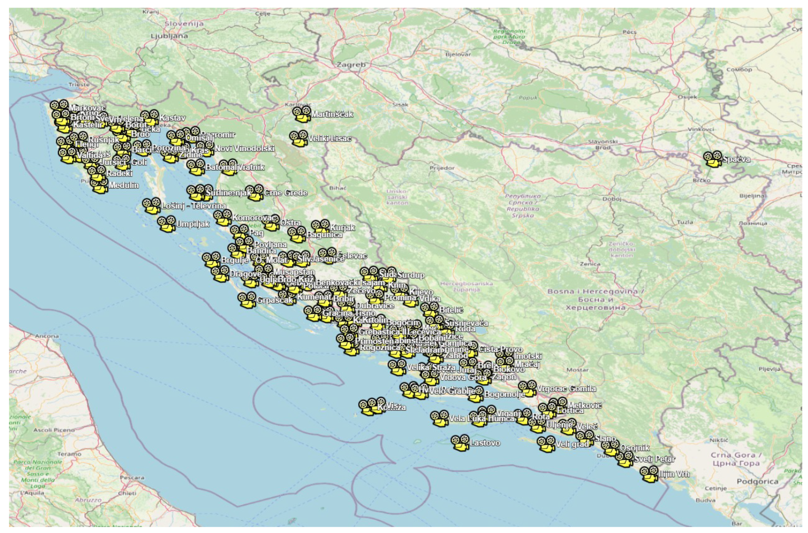
Figure 2.
Examples of wildfire images from the dataset. Images on the left (a, c, e, g) contain first visible signs of smoke that should be automatically detected. In some cases smoke is barely visible. Right column(b, d, f, h): developed wildfire in 3 to 7 minutes from the outbreak.
Figure 2.
Examples of wildfire images from the dataset. Images on the left (a, c, e, g) contain first visible signs of smoke that should be automatically detected. In some cases smoke is barely visible. Right column(b, d, f, h): developed wildfire in 3 to 7 minutes from the outbreak.
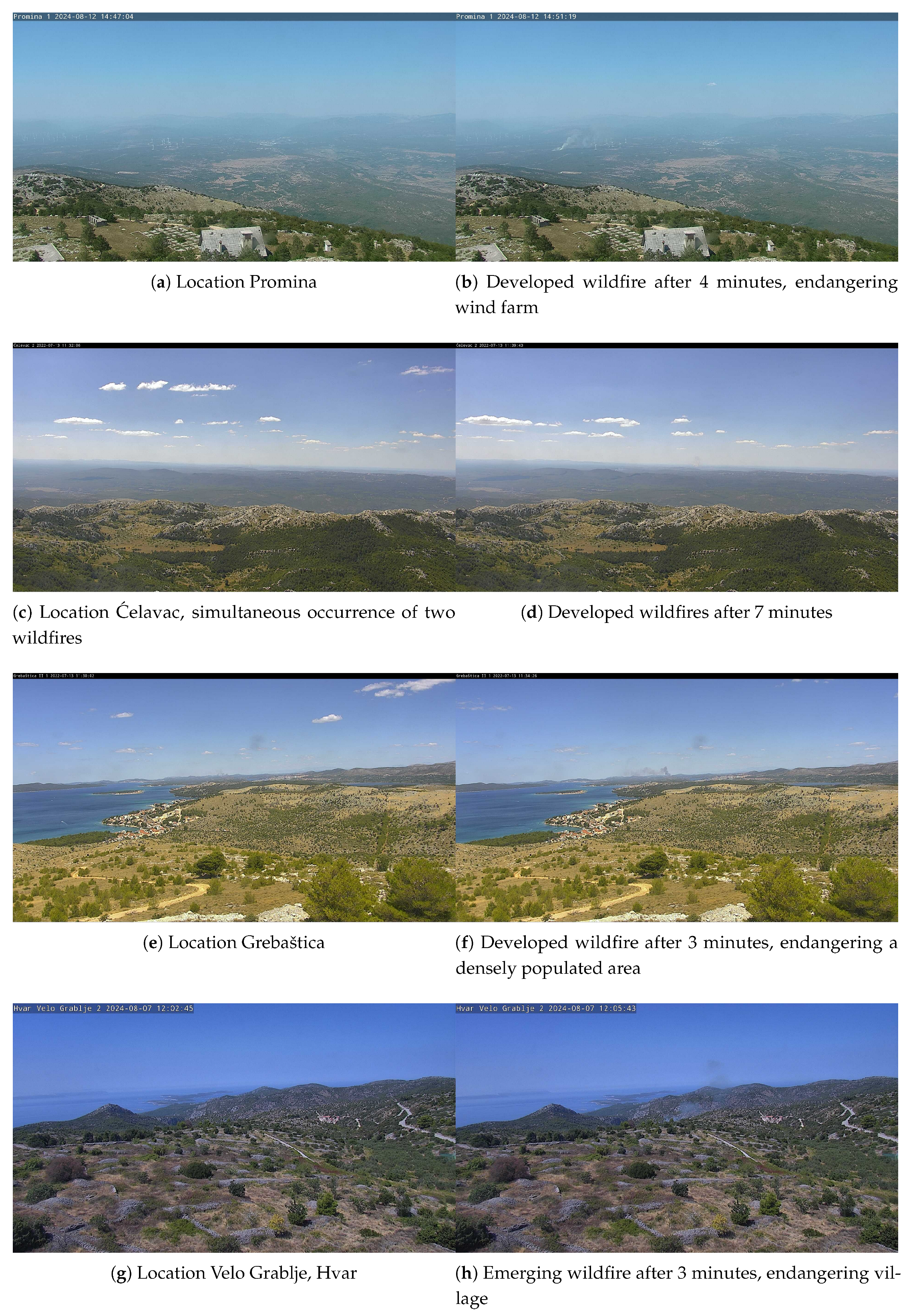
Figure 3.
Short and long term memory channels.
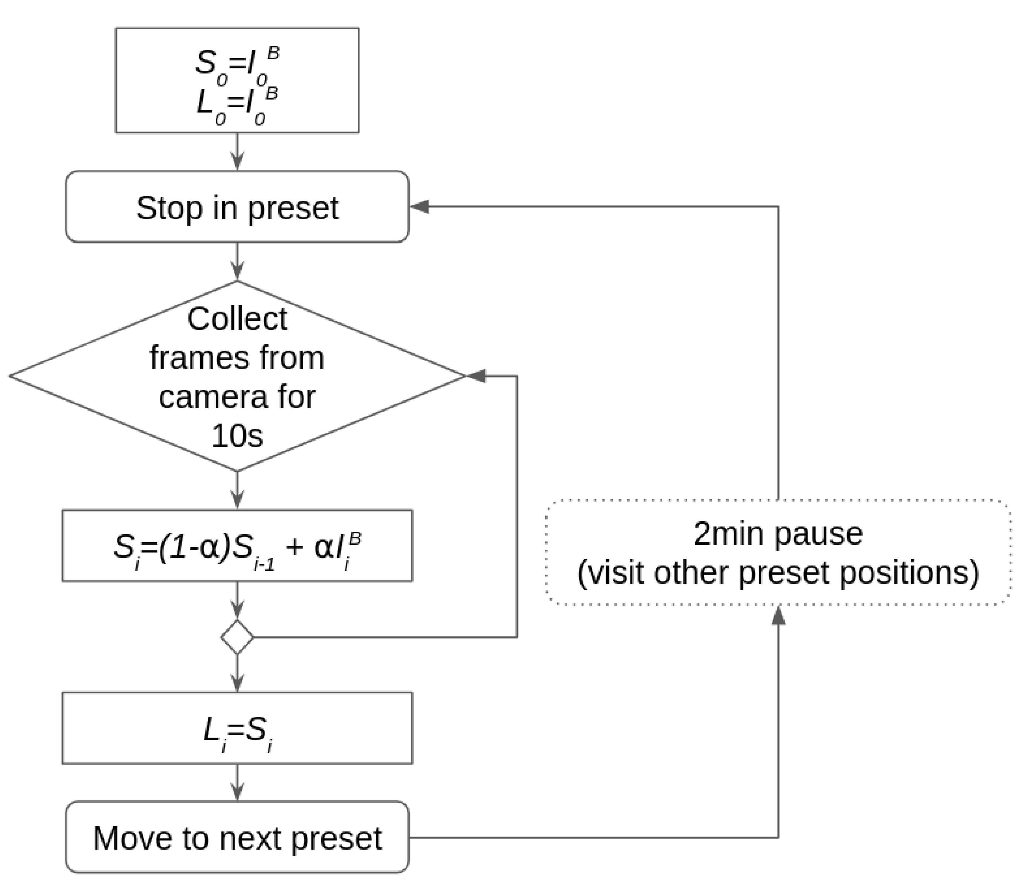
Figure 4.
measure and Average Precision for different multichannel datasets, trained on raw data (no augmentation), evaluated on validation dataset. From left to right: RGB images (3 channels); Temporal image (3 channels); RGB+Temporal image (5 channels); RGB+distance (4 channels); RGB+Temporal+distance (6 channels); RGB+Foreground (5 channels); RGB+Temporal+Foreground+distance (8 channels)
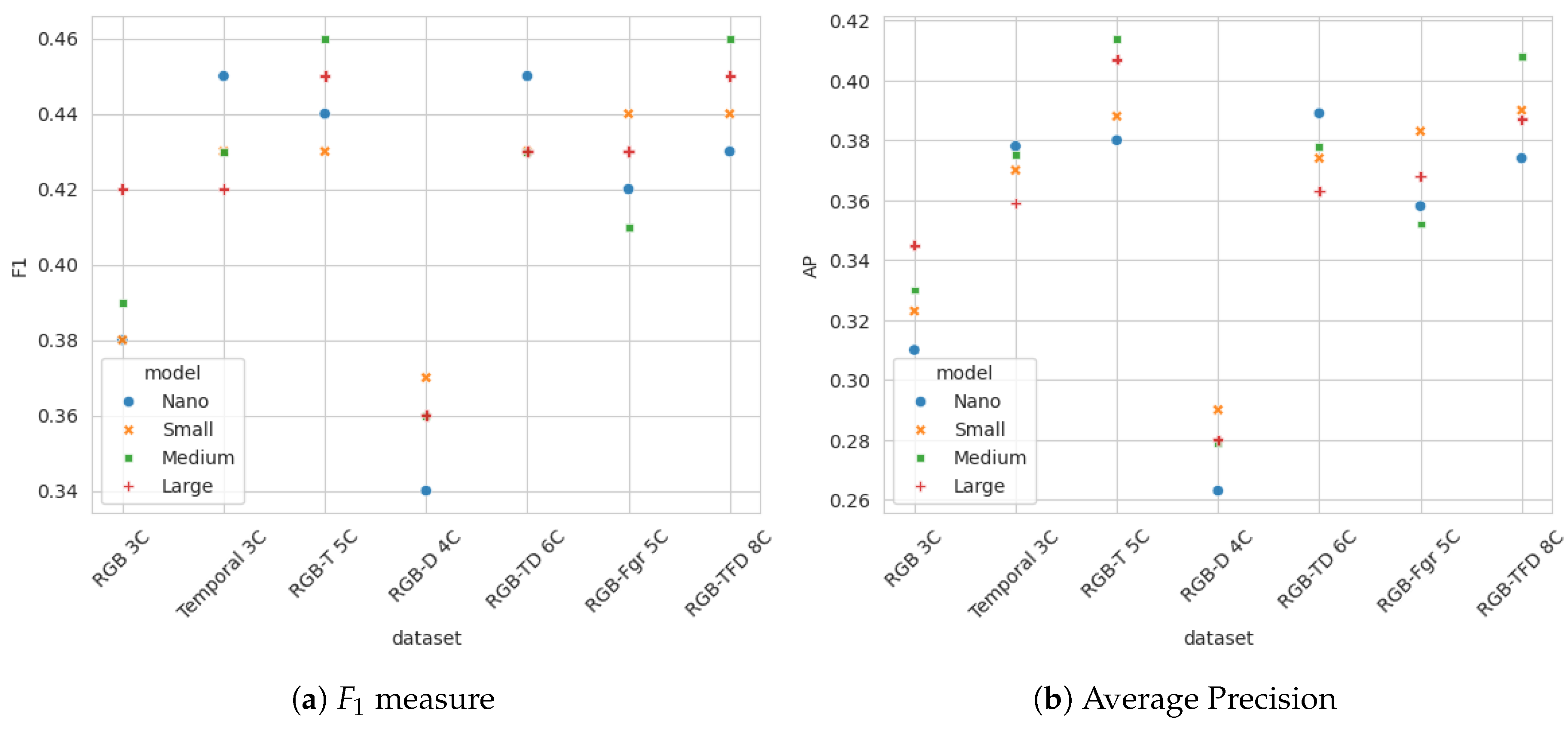
Figure 5.
measure and Average Precision for YOLOv8 spatio-temporal 5 channel, YOLOv8 RGB, YOLOv11 RGB and YOLOv12 RGB trained on augmented data set and evaluated on validation data set.
Figure 5.
measure and Average Precision for YOLOv8 spatio-temporal 5 channel, YOLOv8 RGB, YOLOv11 RGB and YOLOv12 RGB trained on augmented data set and evaluated on validation data set.
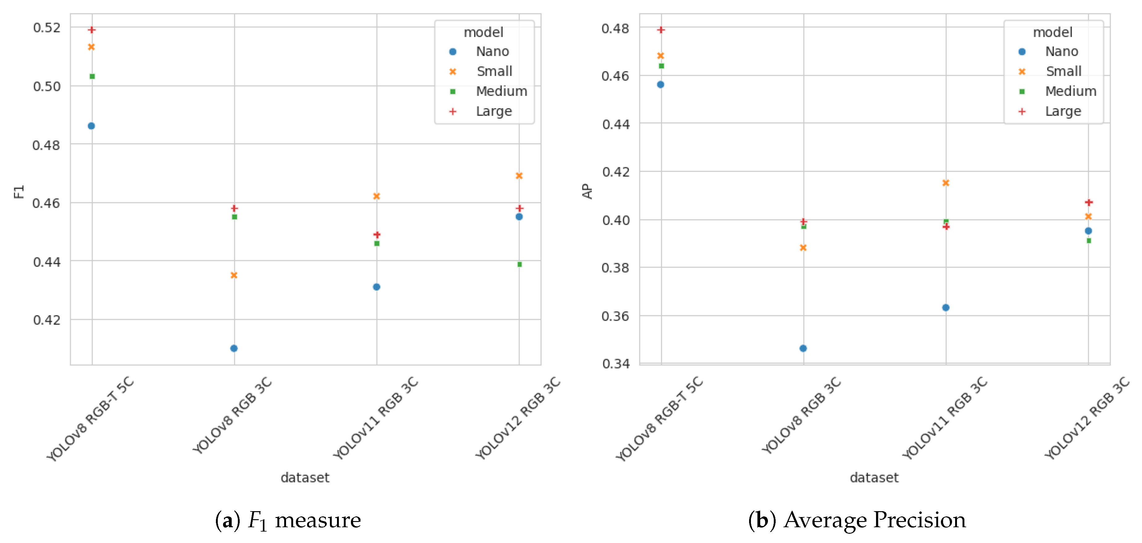
Figure 6.
score for different confidence thresholds for YOLOv8 models trained on 5 channel spatio-temporal data, and YOLOv8, YOLOv11 and YOLOv12 models trained on RGB images. The evaluation results on full-resolution sequences collected from a separate set of surveillance locations (not used for training or validation) are presented.
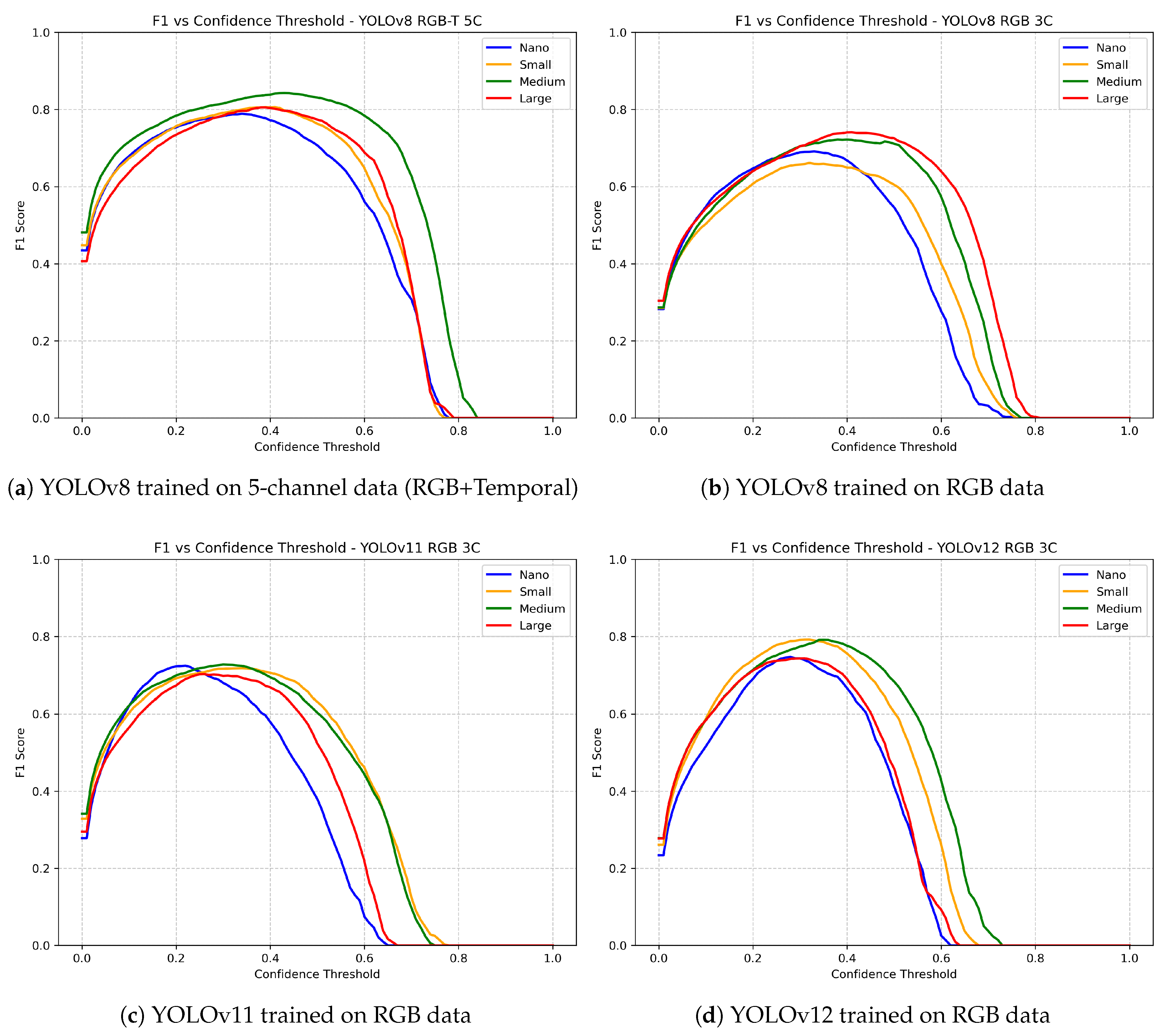
Figure 7.
score vs. inference latency for different data models and YOLO versions. Time in seconds on the x-axis refers to the processing time of a single frame from the full-resolution sequences ().
Figure 7.
score vs. inference latency for different data models and YOLO versions. Time in seconds on the x-axis refers to the processing time of a single frame from the full-resolution sequences ().
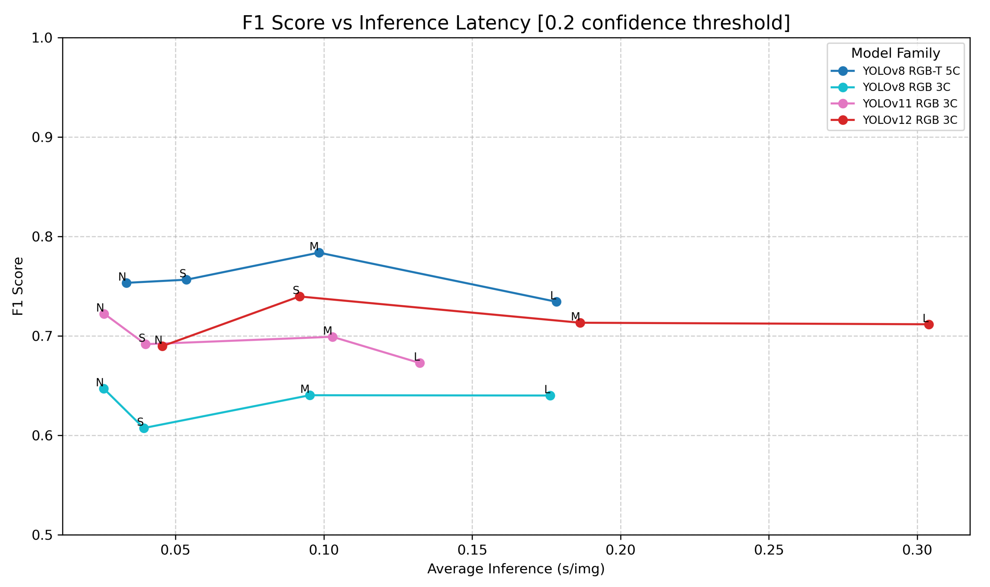

Table 1.
Number of locations and collected sequences for training, validation and test data.
| Data | Locations | Sequences | Smoke | No Smoke |
|---|---|---|---|---|
| Train | 48 | 234 | 147 | 87 |
| Validation | 18 | 53 | 29 | 24 |
| Test | 13 | 46 | 26 | 20 |
Table 2.
Number of extracted 640x640 patches.
| Data | Samples | Smoke | No Smoke |
|---|---|---|---|
| Train (no augmentation) | 9077 | 5238 | 3839 |
| Train (augmented) | 74502 | 37251 | 37251 |
| Validation | 1694 | 847 | 847 |
| Test | 1854 | 927 | 927 |
Table 3.
Augmentation strategies: sequence transform parameters for different transformation in each augmentation pipeline run.
Table 3.
Augmentation strategies: sequence transform parameters for different transformation in each augmentation pipeline run.
| Transformation | 1 | 2 | 3 | 4 | 5 | 6 | 7 |
|---|---|---|---|---|---|---|---|
| Scale | 1.0 | 2.0 | 0.6 | 1.0 | 1.0 | 1.0 | 1.0 |
| Random scale | 0.0 | 0.0 | 0.0 | 0.2 | 0.2 | 0.2 | 0.2 |
| Horizontal flip | 1.0 | 0.2 | 0.2 | 0.2 | 0.2 | 0.2 | 0.2 |
| Rotate | 0.2 | 0.2 | 0.2 | 1.0 | 0.2 | 0.2 | 0.2 |
| Perspective | 0.2 | 0.2 | 0.2 | 0.2 | 0.2 | 1.0 | 0.2 |
| Optical distortion | 0.2 | 0.2 | 0.2 | 0.2 | 1.0 | 0.2 | 0.2 |
| HSV | 0.2 | 0.2 | 0.2 | 0.2 | 0.2 | 0.2 | 0.6 |
| Random brightness | 0.2 | 0.2 | 0.2 | 0.2 | 0.2 | 0.2 | 1.0 |
| Random gamma | 0.2 | 0.2 | 0.2 | 0.2 | 0.2 | 0.2 | 0.6 |
Table 4.
measure for different multichannel datasets, trained on raw data (no augmentation), evaluated on validation data set.
Table 4.
measure for different multichannel datasets, trained on raw data (no augmentation), evaluated on validation data set.
| Num.Ch. | Nano | Small | Medium | Large | |
|---|---|---|---|---|---|
| RGB | 3 | 0.38 | 0.38 | 0.39 | 0.42 |
| Temp. | 3 | 0.45 | 0.43 | 0.43 | 0.42 |
| RGB+T. | 5 | 0.44 | 0.43 | 0.46 | 0.45 |
| RGB+Dist. | 4 | 0.34 | 0.37 | 0.36 | 0.36 |
| RGB+TD | 6 | 0.45 | 0.43 | 0.43 | 0.43 |
| RGB+Fgr. | 5 | 0.42 | 0.44 | 0.41 | 0.43 |
| RGB+TFD | 8 | 0.43 | 0.44 | 0.46 | 0.45 |
Table 5.
Average Precision for different multichannel datasets.
| Num.Ch. | Nano | Small | Medium | Large | |
|---|---|---|---|---|---|
| RGB | 3 | 0.310 | 0.323 | 0.330 | 0.345 |
| Temp. | 3 | 0.378 | 0.370 | 0.375 | 0.359 |
| RGB+T | 5 | 0.380 | 0.388 | 0.414 | 0.407 |
| RGB+Dist. | 4 | 0.263 | 0.290 | 0.279 | 0.280 |
| RGB+TD | 6 | 0.389 | 0.374 | 0.378 | 0.363 |
| RGB+Fgr. | 5 | 0.358 | 0.383 | 0.352 | 0.368 |
| RGB+TFD | 8 | 0.374 | 0.390 | 0.408 | 0.387 |
Table 6.
measure for YOLOv8 trained on 5D spatio-temporal data vs. YOLOv11 and YOLOv12 trained on 3D RGB data, evaluated on validation data set
Table 6.
measure for YOLOv8 trained on 5D spatio-temporal data vs. YOLOv11 and YOLOv12 trained on 3D RGB data, evaluated on validation data set
| Dataset | Nano | Small | Medium | Large | |
|---|---|---|---|---|---|
| YOLOv8 | spatio-temporal 5D | 0.49 | 0.51 | 0.50 | 0.52 |
| YOLOv8 | RGB 3D | 0.41 | 0.44 | 0.46 | 0.46 |
| YOLOv11 | RGB 3D | 0.43 | 0.46 | 0.45 | 0.45 |
| YOLOv12 | RGB 3D | 0.46 | 0.47 | 0.44 | 0.46 |
Table 7.
Average Precision for different multichannel datasets
| Dataset | Nano | Small | Medium | Large | |
|---|---|---|---|---|---|
| YOLOv8 | spatio-temporal 5D | 0.46 | 0.47 | 0.47 | 0.49 |
| YOLOv8 | RGB 3D | 0.35 | 0.39 | 0.40 | 0.40 |
| YOLOv11 | RGB 3D | 0.36 | 0.42 | 0.40 | 0.40 |
| YOLOv12 | RGB 3D | 0.40 | 0.40 | 0.39 | 0.40 |
Table 8.
Successful detections and detection delay. Columns from left to right: TP detections, FN detections, the percentage of TP detections, the number of detections with no delay, mean delay, maximum detection delay for the successful detections.
Table 8.
Successful detections and detection delay. Columns from left to right: TP detections, FN detections, the percentage of TP detections, the number of detections with no delay, mean delay, maximum detection delay for the successful detections.
| RGB-T 5C YOLOv8 |
Detected (TP) |
Missed (FN) |
Rate (%) |
No Delay |
Mean Delay |
Max delay |
|---|---|---|---|---|---|---|
| Nano | 54 | 32 | 62.8 | 44 | 74.4 | 210 |
| Small | 59 | 27 | 68.6 | 48 | 67.3 | 210 |
| Medium | 57 | 29 | 66.3 | 47 | 74.1 | 315 |
| Large | 57 | 29 | 66.3 | 50 | 46.3 | 210 |
|
RGB 3C YOLOv8 |
||||||
| Nano | 56 | 30 | 65.1 | 41 | 77.5 | 315 |
| Small | 55 | 31 | 64.0 | 44 | 96.6 | 316 |
| Medium | 59 | 27 | 68.6 | 50 | 70.6 | 315 |
| Large | 51 | 35 | 59.3 | 42 | 105.6 | 316 |
|
RGB 3C YOLOv11 |
||||||
| Nano | 56 | 30 | 65.1 | 44 | 105.4 | 316 |
| Small | 55 | 31 | 64.0 | 41 | 98.1 | 525 |
| Medium | 51 | 35 | 59.3 | 41 | 84.6 | 525 |
| Large | 53 | 33 | 61.6 | 46 | 45.6 | 105 |
|
RGB 3C YOLOv12 |
||||||
| Nano | 53 | 33 | 61.6 | 44 | 36.2 | 110 |
| Small | 57 | 29 | 66.3 | 52 | 42.6 | 105 |
| Medium | 52 | 34 | 60.5 | 44 | 40.4 | 105 |
| Large | 54 | 32 | 62.8 | 46 | 27.0 | 105 |
Disclaimer/Publisher’s Note: The statements, opinions and data contained in all publications are solely those of the individual author(s) and contributor(s) and not of MDPI and/or the editor(s). MDPI and/or the editor(s) disclaim responsibility for any injury to people or property resulting from any ideas, methods, instructions or products referred to in the content. |
© 2026 by the authors. Licensee MDPI, Basel, Switzerland. This article is an open access article distributed under the terms and conditions of the Creative Commons Attribution (CC BY) license (http://creativecommons.org/licenses/by/4.0/).
Copyright: This open access article is published under a Creative Commons CC BY 4.0 license, which permit the free download, distribution, and reuse, provided that the author and preprint are cited in any reuse.


