
Submitted:
23 February 2026
Posted:
25 February 2026
You are already at the latest version
Abstract
Early detection of battery degradation is essential for ensuring the safety and reliability of electric vehicle (EV) systems under real-world operating variability. This paper proposes a physics-guided multi-sensor learning framework, termed SensorFusion-Former (SFF), for early warning of short-term EV battery performance degradation. The proposed approach integrates a physics-based baseline model for operational normalization, a multi-sensor fusion attention mechanism to model cross-modality interactions, and a lightweight transformer architecture for efficient temporal representation learning. Weak supervision is derived from physics-consistent residual analysis with temporal smoothing, enabling scalable training without dense manual annotations. To support reliable deployment, evidential uncertainty modeling and conformal calibration are incorporated to obtain statistically controlled decision thresholds. Experiments conducted on a real driving cycle dataset from IEEE DataPort demonstrate that SFF consistently outperforms classical machine learning methods, deep neural networks, and standard transformer models in terms of early-warning lead time, false alarm rate, and inference efficiency, while maintaining competitive discriminative performance. Cross-scenario evaluations under diverse thermal conditions further confirm the robustness and generalization capability of the proposed framework.
Keywords:
electric vehicle batteries
; short-term performance degradation
; early warning systems
; physics-guided learning
; multi-sensor data fusion
; transformer-based time-series modeling
; battery health monitoring
; uncertainty-aware prediction
1. Introduction
The global transition toward electric vehicles (EVs) has substantially reshaped the automotive sector, with lithium-ion batteries serving as the core technology governing driving range, operational safety, and total cost of ownership [1]. Extensive prior research has investigated long-term battery degradation phenomena, including capacity fade, impedance growth, and cycle-life prediction [2,3]. In contrast, the detection of short-term performance degradation during real-world vehicle operation remains comparatively underexplored. Such short-term degradation events, including transient voltage drops, abrupt increases in effective internal resistance, and temporary power delivery limitations, may develop within hours or days due to aggressive driving behavior, fast charging, or rapid thermal fluctuations [4]. Although many of these effects are partially reversible, their occurrence can reduce driver confidence, impair accurate state-of-charge (SoC) estimation, and potentially accelerate irreversible battery aging if not identified and mitigated in a timely manner.
Early detection of short-term battery degradation poses several fundamental technical challenges. Modern EV fleets exhibit pronounced heterogeneity in battery chemistries, vehicle platforms, and operating environments, resulting in highly variable electrical and thermal load profiles. Furthermore, labeled degradation events are inherently scarce, as many abnormal behaviors do not trigger battery management system (BMS) diagnostic codes until significant deterioration has already occurred. Any on-board detection strategy must therefore operate in real time using only signals routinely available from the BMS and the controller area network (CAN), including terminal voltage, current, SoC, battery and ambient temperatures, and auxiliary power consumption. Approaches that rely on controlled excitation or predefined test sequences are thus impractical for naturalistic driving conditions. From a safety-critical deployment perspective, accurate detection alone is insufficient; decision mechanisms must also provide quantifiable and risk-controlled guarantees, particularly with respect to false-negative outcomes that may allow hazardous conditions to persist undetected.
Existing battery monitoring and anomaly detection methods can be broadly categorized as physics-based, data-driven, or hybrid approaches. Physics-based techniques, such as equivalent circuit models (ECMs) and electrochemical impedance spectroscopy (EIS), offer interpretable estimates of internal resistance and diffusion-related parameters [5,6]. However, these methods typically assume idealized current excitation patterns that rarely occur in real driving, rendering parameter estimation from naturalistic data sparse, noisy, and highly dependent on operating conditions. Data-driven methods, including support vector machines, random forests, and recurrent neural networks [7,8], are capable of capturing complex nonlinear sensor relationships but often lack physical grounding. As a result, they may misinterpret normal operational variability as degradation and exhibit limited robustness under distribution shifts. Hybrid approaches [9,10] partially address these limitations, yet many still depend on explicit current step detection, underutilize multi-sensor information, and do not provide formal guarantees on decision risk.
These limitations motivate the development of a physics-guided, multi-sensor learning framework that is explicitly designed for real-time deployment under realistic operating conditions. This paper addresses the problem of early warning for short-term EV battery performance degradation, with an emphasis on detection timeliness, robustness, and computational efficiency, rather than pointwise anomaly classification accuracy alone. The main contributions of this work are summarized as follows:
- Physics-guided early warning framework. We propose a physics-guided multi-sensor learning framework, termed SensorFusion-Former (SFF), that integrates a physics-based baseline model with data-driven temporal learning. The physics model normalizes operational variability, allowing the learning architecture to focus on degradation-relevant residual dynamics instead of nominal operating fluctuations.
- Multi-sensor fusion with efficient temporal modeling. A multi-sensor fusion attention mechanism is introduced to explicitly capture cross-modality interactions among electrical, thermal, and auxiliary signals. This mechanism is combined with a lightweight transformer architecture to achieve effective temporal representation learning while maintaining low inference latency suitable for real-time battery management systems.
- Weakly supervised learning without dense annotations. A weak supervision strategy based on physics-consistent residual analysis and temporal smoothing is developed, enabling scalable model training without the need for densely labeled degradation events. This approach substantially reduces annotation cost while preserving early-warning sensitivity.
- Risk-aware decision making via uncertainty calibration. To enhance deployment reliability, evidential uncertainty modeling and conformal calibration are incorporated into the early warning head, yielding statistically controlled decision thresholds with bounded false alarm risk under distributional variability.
- Comprehensive evaluation across early-warning dimensions. Extensive experiments conducted on a real driving cycle dataset from IEEE DataPort demonstrate that the proposed framework consistently outperforms classical machine learning methods, deep neural networks, and standard transformer models. The proposed approach achieves superior early-warning lead time and lower false alarm rates, while maintaining competitive discriminative performance and reduced inference latency across diverse thermal operating scenarios.
The remainder of this paper is organized as follows. Section 2 reviews prior work on battery health diagnostics and fault detection, multi-sensor fusion and deep learning architectures, uncertainty-aware decision-making, and physics-guided machine learning for battery systems. Section 3 presents the proposed system model and algorithms, including the multi-sensor problem formulation, the physics-guided surrogate voltage model, the SensorFusion-Former architecture, probabilistic multi-task prediction heads, the unified training objective, and the complete training and deployment pipeline, together with an analysis of computational complexity and real-time feasibility. Section 4 reports the experimental setup and a comprehensive evaluation of the proposed approach, covering overall comparisons with baseline models, ablation studies, cross-scenario generalization across diverse thermal domains, and early warning capability analysis. Finally, Section 5 concludes the paper and outlines directions for future work.
2. Related Work
Accurate detection and early warning of short-term battery performance degradation in electric vehicles require addressing several interrelated technical challenges, including modeling nonlinear electro-thermal dynamics, integrating heterogeneous sensor streams, quantifying predictive uncertainty, and maintaining robustness across diverse operating conditions [11]. This section reviews relevant literature in four closely related areas: battery health diagnostics and fault detection, multi-sensor fusion and deep learning architectures for time-series analysis, uncertainty quantification and risk-controlled decision-making, and physics-guided machine learning for battery systems.
2.1. Battery Health Diagnostics and Fault Detection
Battery health monitoring for electric vehicles has traditionally followed model-based, data-driven, and hybrid paradigms. Model-based approaches, such as ECMs and electrochemical formulations including the Doyle–Fuller–Newman (DFN) model [12,13,14], provide interpretable physical parameters but typically rely on controlled excitation protocols, such as pulse tests or electrochemical impedance spectroscopy [15,16]. These requirements are difficult to satisfy during naturalistic driving, where current profiles are highly irregular. As a result, parameter estimates obtained under dynamic conditions tend to be sparse, noisy, and sensitive to operating points, limiting their suitability for real-time deployment.
Data-driven methods infer degradation patterns directly from operational data. Early studies employed classical machine learning techniques, including support vector machines and random forests [17,18], while more recent work has adopted deep learning architectures such as convolutional neural networks (CNNs), recurrent neural networks (RNNs), and long short-term memory (LSTM) models [19,20,21]. These approaches have improved temporal modeling capability and enabled large-scale anomaly detection [22,23]. However, most existing studies focus on long-term health indicators, including state-of-health (SOH) and remaining useful life (RUL) [24,25], rather than short-term transient anomalies that occur over minutes or hours. Such short-term events, including abrupt resistance increases or localized thermal excursions, require operation-normalized and high-resolution indicators. In addition, labeled fault data remain limited because early-stage anomalies often do not trigger diagnostic codes within battery management systems [26,27].
2.2. Multi-Sensor Fusion and Deep Learning Architectures
Modern battery management systems continuously collect electrical, thermal, and operational signals. Despite this availability, many diagnostic models process individual sensor channels independently or rely on simple feature concatenation. Recent studies have demonstrated that explicit multi-sensor fusion can substantially improve diagnostic performance. For example, Liu et al. [28] showed that integrating multi-modal field data from large EV fleets significantly enhances SOH estimation accuracy, emphasizing the importance of modeling electro-thermal interactions.
Advances in sequence modeling have led to increasing adoption of transformer architectures for battery analytics due to their ability to capture long-range temporal dependencies [29]. Transformer-based models have demonstrated improved SOH prediction performance compared with recurrent architectures [30], and hybrid designs, such as transformer–LSTM models, have been explored for fast-charging scenarios [31]. Nevertheless, most existing transformer-based approaches focus on encoder-only designs, lack physics-guided conditioning, and rarely perform structured multi-sensor tokenization. Hybrid CNN–transformer models [32,33] combine local transient feature extraction with global temporal modeling, but typically fuse modalities only after independent feature processing rather than through explicit cross-sensor attention mechanisms.
2.3. Uncertainty Quantification and Risk-Controlled Decision-Making
A major limitation of existing battery diagnostic models lies in the absence of principled uncertainty quantification suitable for safety-critical applications. Most deep learning methods produce deterministic point estimates without conveying predictive confidence [34]. Bayesian approaches, including Monte Carlo dropout and variational inference [35,36], can provide uncertainty estimates but incur substantial computational overhead and require careful prior specification. Gaussian process regression offers probabilistic predictions [37,38], yet its scalability remains limited for large-scale battery datasets.
Conformal prediction [39] has emerged as a distribution-free alternative that provides finite-sample coverage guarantees. Recent applications to SOH and RUL forecasting [40] have demonstrated its effectiveness in generating calibrated prediction intervals across different models. However, existing studies primarily address long-term regression tasks and do not consider short-term anomaly detection or risk-controlled classification, where false-negative rates must be explicitly bounded in deployment settings.
Weighted conformal calibration [41,42] further addresses distribution shift by assigning importance weights to calibration samples based on domain similarity, which is particularly relevant for EV fleets operating under seasonal and usage variability. To the best of our knowledge, no prior work has integrated weighted conformal calibration with deep sequence models for battery anomaly detection or provided unified, risk-controlled decision thresholds for both regression and classification tasks.
2.4. Physics-Guided Machine Learning for Battery Systems
To mitigate the limited interpretability and domain robustness of purely data-driven models, recent research has explored physics-guided and hybrid machine learning approaches. Many studies incorporate parameters derived from equivalent circuit models, such as ohmic and polarization resistance, as auxiliary inputs or learning targets [43,44]. These methods, however, often depend on explicit current-step detection, which becomes unreliable under highly dynamic driving conditions.
Scientific machine learning approaches, including physics-informed neural networks (PINNs) [45,46], embed governing electrochemical equations into neural network training to improve extrapolation to unseen operating regimes. For example, Murgai et al. [47] demonstrated enhanced degradation modeling using universal differential equations. While effective, such methods typically require detailed knowledge of system equations and incur nontrivial computational cost.
A complementary physics-guided strategy, adopted in this work, employs a grey-box voltage baseline that predicts expected terminal voltage from state-of-charge, temperature, and current using constrained shape-prior models. The normalized residual between measured and baseline voltage provides a continuous and operation-invariant indicator of short-term degradation without requiring explicit step detection. Although related concepts have been explored for open-circuit-voltage-based state-of-charge correction [48], they have not been systematically extended to short-term degradation detection within multi-sensor deep learning frameworks.
Despite substantial progress in battery diagnostics and time-series learning, several critical gaps remain. Most existing methods emphasize long-term metrics such as SOH and RUL rather than short-term transient anomalies. Multi-sensor fusion is often implemented through simple feature concatenation without explicit cross-channel attention. Transformer architectures have seen limited development for physics-guided battery monitoring and rarely support causal, streaming-friendly inference. Uncertainty quantification remains either ad hoc or computationally demanding, and risk-controlled conformal calibration has not been explored for battery anomaly detection. Physics-guided approaches typically rely on sparse step-based parameter estimation or assume full knowledge of governing electrochemical equations.
This work addresses these gaps by introducing a physics-guided continuous degradation surrogate that eliminates the need for step detection, a multi-sensor fusion transformer architecture (SensorFusion-Former) with explicit cross-sensor attention and causal temporal modeling using efficient FAVOR+ kernels, probabilistic multi-task heads for degradation severity estimation and evidential classification, and weighted conformal calibration for deriving risk-controlled decision thresholds. Together, these contributions enable early detection of short-term battery degradation with principled uncertainty quantification, real-time feasibility, and robustness to distribution shifts, which are essential for safe and scalable deployment in electric vehicle fleets.
3. System Model and Algorithms
This section presents the proposed system for early detection of short-term performance degradation in EV lithium-ion batteries. The system operates on routinely logged vehicle telemetry and consists of three key components: construction of physics-guided surrogate targets, derivation of weak degradation labels, and training of a multi-sensor deep learning model that produces calibrated and risk-controlled early warning alerts.
Figure 1 illustrates an overview of the proposed system architecture. The framework comprises four main stages. First, multi-sensor data ingestion is performed together with a physics-guided baseline model to normalize operating conditions (left). Second, the SensorFusion-Former model processes the normalized inputs through seven internal layers, including cross-sensor attention, physics-conditioned biasing, and causal temporal attention based on FAVOR+ kernels (center). The core methodological innovations are highlighted using orange blocks and marked with the symbol ★. Third, multi-task probabilistic prediction heads generate outputs for degradation regression, event classification, early warning, and physics-consistency forecasting (right). Finally, offline training and conformal calibration pipelines are employed to enable domain adaptation and risk-controlled deployment (bottom).
The proposed methodology is built upon three core design components. First, the cross-sensor attention module (Layer 1) captures instantaneous inter-domain dependencies among electrical, thermal, and auxiliary sensor groups. Second, physics-conditioned biasing (Layer 2) injects grey-box model outputs, including the voltage residual , the reference voltage , and the ohmic resistance estimate , into the latent representations without introducing future information leakage. Third, causal temporal attention based on FAVOR+ kernels (Layers 4–6) achieves a computational complexity of , enabling real-time inference in embedded battery management systems while preserving expressive attention modeling. Table 1 summarizes the key symbols used in the problem formulation, physics-based modeling, and architectural design.
3.1. Multi-Sensor Problem Formulation
At each discrete time index with sampling interval , the battery management system observes a multi-sensor feature vector
where denotes electrical signals, denotes thermal signals, and denotes auxiliary operational signals, with .
Specifically, the electrical channel vector is defined as , including terminal voltage , current , state-of-charge , and traction power . The thermal channel vector captures battery temperature , ambient temperature , and coolant mass flow rate . The auxiliary channel vector includes power consumption of the heating, ventilation, and air conditioning system , heating power , vehicle speed , and longitudinal acceleration .
Each sensor group provides complementary information about battery operation. The electrical signals reflect the instantaneous electrochemical response of the battery, the thermal signals capture temperature-dependent reaction kinetics and aging mechanisms, and the auxiliary signals describe external load conditions and vehicle usage patterns that indirectly influence battery stress. This structured multi-sensor representation enables the model to differentiate between benign operational effects, such as transient voltage drops during aggressive acceleration, and potential degradation signatures, such as sustained increases in internal resistance under moderate load conditions.
Direct interpretation of raw sensor measurements is challenging due to their strong dependence on operating context, including state-of-charge, temperature, and instantaneous power demand. For example, a voltage drop of several volts may be expected at high discharge rates and low ambient temperatures, yet indicate abnormal behavior under moderate load at nominal conditions. To decouple operation-induced variability from degradation-related effects, a physics-guided baseline model is introduced in the following subsection.
3.2. Physics-Guided Surrogate Voltage Model
Direct interpretation of raw voltage deviations is difficult because observed variations may be caused by benign operating factors, including load transients, temperature changes, and SoC dependence, rather than true degradation. To separate operating effects from degradation-related behavior, we introduce a grey-box, physics-guided surrogate voltage model that approximates the expected pack voltage under nominally healthy conditions. The resulting reference voltage serves as a baseline for constructing operation-normalized deviation signals.
3.2.1. Three-Component Voltage Decomposition
We express the reference pack voltage as the sum of three physically interpretable components:
where denotes the monotone non-decreasing open-circuit-voltage (OCV) surface that characterizes the equilibrium potential and satisfies . The term is a non-negative ohmic resistance map governing the instantaneous current-induced voltage drop. The dynamic component is modeled as a stable and causal filtering operator that captures time-dependent polarization and diffusion effects driven by the recent excitation history .
The parameter set collects the learnable coefficients of the three components. We estimate from nominally healthy operation segments by solving
where is the Huber loss and imposes soft shape constraints to preserve monotonicity of and non-negativity of . The regularization weight balances data fit and physical plausibility.
Figure 2 illustrates the decomposition on a representative driving segment. The OCV surface captures equilibrium voltage variation with SoC and temperature, the ohmic term explains instantaneous losses that scale with current, and the dynamic term accounts for polarization and diffusion effects driven by recent current and temperature history.
As shown in Figure 2(a), the reference voltage closely tracks the measured voltage over diverse operating regimes during healthy operation, including high discharge at low temperature, moderate load at nominal temperature, and regenerative braking. Fitting the surrogate using (3) produces a reference trajectory that accounts for expected variations induced by SoC evolution, thermal conditions, and load changes, so that residual deviations become more indicative of abnormal behavior.
During the degradation episode, a persistent discrepancy emerges between and that cannot be explained by the calibrated healthy baseline. Such unexplained deviations may reflect increased effective internal resistance or abnormal polarization dynamics and therefore motivate an operation-normalized residual, since the magnitude of is strongly dependent on current level.
3.2.2. Operation-Normalized Residual and Severity Index
To quantify deviations in a manner robust to operating variability, we define the operation-normalized residual
where prevents numerical instability under near-zero current conditions. The normalization scales the absolute deviation by the predicted ohmic drop, so reflects relative unexplained losses rather than raw voltage magnitude.
Figure 2(b) validates this design. Despite large voltage excursions caused by acceleration, coasting, and regenerative braking, the residual remains consistently small during healthy operation, indicating effective suppression of operation-induced confounders. In contrast, during the degradation episode, increases markedly and exceeds the threshold , enabling clear separation between degradation-related behavior and benign operating variability. The highlighted region where is later converted into frame-level labels via the temporal smoothing procedure in the next subsection.
The early-warning interval in Figure 2(b) illustrates the intended predictive setting. Specifically, for a horizon of H samples, the model is trained to predict both reactive event labels and early-warning labels (defined in Section 3.2.3), enabling alerting prior to the onset of a confirmed event.
Single-sample residuals may be noisy and influenced by short-lived transients. We therefore define a windowed severity index over a horizon of length :
where denotes the Huber function
with . The weights emphasize operating points that are informative for degradation assessment. In practice, is derived from a kernel density estimate in the space: operating regimes that occur frequently under healthy conditions are down-weighted, whereas rarer but diagnostically informative regimes receive higher weight.
The resulting summarizes recent operation-normalized deviations in a manner that is robust to outliers while remaining sensitive to sustained abnormal behavior. This scalar sequence serves as the primary signal for automatic event label generation.
3.2.3. Event Labeling with Hysteresis and Early Warning
Since ground-truth labels for short-term degradation events are rarely available, we construct weak labels from the severity index . A degradation threshold is calibrated on healthy data as
where denotes the empirical -quantile with , ensuring that only a small fraction of healthy samples exceed .
Raw frame-level flags are defined as
where filters out low-current intervals that are typically less informative.
To reduce spurious detections induced by sensor noise and transient fluctuations, we apply three post-processing operations. First, a hysteresis rule enforces temporal consistency by confirming an event only after at least consecutive samples satisfy . Second, candidate segments shorter than samples are removed. Third, neighboring segments separated by gaps no larger than samples are merged, preventing a single anomaly from being fragmented into multiple detections.
These steps address complementary failure modes of threshold-based detection. Hysteresis suppresses isolated spikes, the minimum-duration constraint removes short-lived artifacts, and gap merging consolidates fragmented segments caused by varying current magnitude. Together, the procedure balances sensitivity and false-alarm robustness and yields event intervals that better correspond to physically meaningful degradation episodes.
Figure 3 shows how raw threshold crossings are refined into coherent event intervals and corresponding early-warning windows. After post-processing, we obtain a set of J disjoint event intervals , where and denote the start and end indices of the jth event. The binary event label is defined as
and the H-step early-warning label is defined as
The early-warning label marks samples within H steps prior to event onset, enabling the model to learn predictive precursors rather than only reactive detection.
3.3. SensorFusion-Former Architecture
3.3.1. Sensor-Group Tokenization
For each sensor group and time index t, we map group-specific inputs to a shared latent space via
where denotes layer normalization, is a group-specific feedforward network, and is a learnable group embedding. This design preserves modality-specific characteristics while enabling subsequent cross-group interaction modeling in a common representation space.
3.3.2. Cross-Sensor Attention
To capture instantaneous dependencies among sensor groups, we concatenate the group embeddings and apply multi-head self-attention (MHSA):
Here, denotes a multi-head self-attention operator applied over the group tokens at the same time step. The fused token summarizes cross-sensor interactions and serves as the input to subsequent temporal modeling.
3.3.3. Physics-Conditioned Feature Injection
To incorporate physics-guided information without violating causality, we inject grey-box outputs through a learned conditioning function:
where is a lightweight multilayer perceptron (MLP). The conditioning variables are computed from current and past observations only; therefore, the injection does not introduce future information leakage.
3.3.4. Causal Temporal Modeling with FAVOR+
To model temporal dependencies over a causal window of length W, we construct a context matrix
The sequence is processed by L causal transformer blocks:
where each block implements causal attention to prevent access to future tokens.
Standard self-attention requires computing all pairwise similarities within a length-W window, which incurs time complexity and memory. Such quadratic scaling can become a deployment bottleneck when streaming inference is required on resource-constrained battery management systems.
To improve efficiency, we adopt FAVOR+ (Fast Attention Via positive Orthogonal Random features) attention [49], which approximates softmax attention using random feature maps. This yields linear complexity with memory , where r denotes the number of random features. Table 2 summarizes the computational and memory complexity of FAVOR+ relative to representative efficient attention variants.
Finally, we aggregate the temporal context into a single latent representation:
where can be implemented using the last token, global average pooling, or attention-weighted pooling. In our implementation, we use the last token to preserve causality and to emphasize the most recent context.
3.4. Probabilistic Multi-Task Prediction Heads
The proposed architecture employs probabilistic multi-task prediction heads to jointly estimate degradation severity, event occurrence, and early-warning likelihood, while explicitly modeling prediction uncertainty. This design enables risk-aware decision-making and supports subsequent conformal calibration.
3.4.1. Heteroscedastic Regression for Severity
To model both the expected value and uncertainty of degradation severity, we adopt a heteroscedastic regression formulation. Specifically, the predictive mean and variance are given by
where denotes the predicted mean severity and represents the input-dependent predictive variance.
The regression loss is defined as the negative log-likelihood of a Gaussian distribution:
where is the degradation severity index defined in Section 3.2, and are sample-specific weights that reflect the operating-point density introduced in Section 3.2. This formulation penalizes both large prediction errors and overconfident uncertainty estimates.
3.4.2. Evidential Classification
For binary event detection, we employ an evidential classification framework based on the Beta-Bernoulli model, which provides a principled representation of epistemic uncertainty. The parameters of the Beta distribution are predicted as
ensuring and for numerical stability. The resulting predictive event probability is given by
and the associated predictive variance is
which serves as a measure of epistemic uncertainty.
The evidential classification loss combines data fidelity and uncertainty regularization:
where denotes the binary cross-entropy loss, is the event label defined in Section 3.2.3, and controls the strength of uncertainty regularization. This objective encourages accurate predictions while discouraging unwarranted overconfidence.
An analogous evidential formulation is applied to early-warning prediction. Specifically, a separate classification head with parameters is trained using the corresponding early-warning labels , yielding an early-warning probability and loss defined in the same manner.
3.5. Risk-Controlled Decision Making via Weighted Conformal Prediction
To provide finite-sample performance guarantees under distributional variability, we adopt a weighted conformal calibration strategy on a held-out calibration set . The use of sample-dependent weights allows the calibration procedure to account for nonuniform operating conditions commonly observed in real-world electric vehicle data.
3.5.1. Regression Calibration
For degradation severity prediction, we compute a weighted conformal quantile based on normalized regression residuals:
where denotes the weighted quantile operator and are sample-specific weights proportional to the local data density in the operating-condition space. This calibration ensures that the normalized residual exceeds with probability at most on unseen data drawn from a similar distribution.
During deployment, a severity exceedance is declared whenever
thereby yielding a risk-controlled decision rule with a finite-sample guarantee.
3.5.2. Classification Calibration
For event detection, we determine a probability threshold that explicitly controls the false-negative rate at level . The threshold is selected on the calibration set as
where denotes the calibrated predictive probability. This procedure yields a data-driven decision threshold that bounds the empirical false-negative rate on the calibration set and supports risk-aware deployment.
3.6. Unified Training Objective
The complete training objective integrates all learning components into a single loss function:
where , , , , and are nonnegative weighting coefficients that balance the contributions of each loss term.
The physics-consistency loss
encourages consistency between the learned representations and the underlying voltage dynamics by penalizing discrepancies in next-step voltage prediction.
In addition, a contrastive learning component
implements an InfoNCE objective over temporally adjacent windows, where and denote representations of positive temporal pairs, is the batch set of candidate keys, and is the contrastive temperature. This term promotes temporal consistency and improves representation quality for downstream prediction tasks.
Model optimization is performed using the AdamW optimizer with gradient clipping (norm bounded by 1.0), cosine learning-rate decay, and mixed-precision training to improve numerical stability and computational efficiency.
3.7. Training and Deployment Algorithm
Algorithm 1 integrates all components of the proposed framework into a unified training and deployment workflow. The procedure starts by estimating the parameters of the physics-based baseline model, denoted by , using nominally healthy data according to Eq. (3). Based on the trained baseline, operation-normalized residuals and degradation severity indices are computed for the full dataset. A degradation threshold is then calibrated, and the corresponding temporal event labels are generated using the temporal smoothing strategy described in Section 3.2.3.
The SensorFusion-Former model is subsequently trained under the unified multi-task objective in Eq. (28). Optimization is performed using the AdamW optimizer with gradient clipping and early stopping to promote stable convergence. After model training, weighted conformal calibration is conducted on the held-out calibration set to estimate the conformal quantile and the probability thresholds . These calibrated quantities are used during deployment to enable risk-controlled decision making for both severity assessment and event detection.
| Algorithm 1: SensorFusion-Former Training and Calibration |
|
3.8. Computational Complexity and Real-Time Feasibility
We analyze the computational requirements of the proposed SensorFusion-Former architecture to assess its suitability for real-time deployment in embedded BMS with limited computational resources.
Theorem 1
(Per-Step Inference Complexity). Consider a causal context window of length W, hidden dimension , L transformer layers, H attention heads, and FAVOR+ rank r. The per-step forward-pass computational complexity of the proposed model is given by
where the three terms correspond to sensor-group tokenization and fusion, linearized causal attention, and position-wise feedforward networks, respectively.
Proof.
The overall complexity is derived by analyzing each component of the forward pass. First, cross-sensor attention operates over sensor groups. Computing group-wise projections and attention incurs operations, which simplifies to and is negligible compared with temporal modeling costs. Second, each FAVOR+ causal attention layer processes a sequence of length W with hidden dimension using r random features per attention head, resulting in operations per layer. Third, the position-wise feedforward networks require operations per layer. Summing these terms over L layers yields the stated complexity. Since by design, the overall complexity scales linearly with the window length W. □
For comparison, a standard transformer with vanilla self-attention incurs a per-step complexity of , which is dominated by the quadratic dependence on the sequence length. Under typical deployment settings (e.g., , , , , and ), the FAVOR+ attention mechanism reduces the attention-related computation by more than an order of magnitude relative to vanilla attention, while preserving the expressive power of softmax-based attention.
The resulting linear scaling with respect to W enables real-time inference at a sampling interval of ms on embedded platforms commonly used in automotive battery management systems. This computational efficiency leaves sufficient headroom for concurrent BMS tasks, including state estimation, thermal control, and safety monitoring, thereby supporting practical on-board deployment.
3.9. Complete Methodology Pipeline
Figure 4 provides an integrated overview of the proposed methodology by connecting all components introduced in this section into a unified processing pipeline. The workflow begins with the estimation of the physics-guided baseline model parameters using nominally healthy telemetry data according to Eq. (3). This stage establishes reference voltage predictions and operation-normalized residuals , which form the foundation for subsequent degradation quantification.
In the second phase, weak supervision signals are constructed by computing the degradation severity index , calibrating the degradation threshold , and applying temporal smoothing operations, including hysteresis, minimum-duration filtering, and gap merging. These steps yield both frame-level event labels and horizon-based early-warning labels , enabling the learning of both reactive detection and predictive warning capabilities.
The third phase trains the SensorFusion-Former model using the unified multi-task objective defined in Eq. (28). This objective jointly optimizes heteroscedastic regression for severity estimation, evidential classification for event detection and early warning, and physics-consistency forecasting through next-step voltage prediction. Model optimization is performed using the AdamW optimizer with gradient clipping and early stopping to ensure stable and robust convergence.
In the final phase, weighted conformal prediction is applied on a held-out calibration set to derive risk-controlled decision thresholds, including the conformal quantile and probability threshold . The calibrated model is then deployed for real-time inference on-board electric vehicles.
As illustrated by the red dashed feedback loop in Figure 4, the proposed pipeline supports continuous post-deployment refinement. Newly collected fleet-scale data can be used to update domain-alignment and calibration components, allowing the system to maintain robustness under seasonal variability, usage-pattern shifts, and platform drift, with updated parameters periodically redistributed across the vehicle fleet.
4. Experimental Evaluation
4.1. Experimental Setup
4.1.1. Dataset Description
All experiments are conducted using the Battery and Heating Data in Real Driving Cycles dataset released on IEEE DataPort [53]. This dataset provides second-by-second CAN telemetry collected under real-world driving conditions and spans a wide range of operating regimes relevant to electric vehicle battery health monitoring.
The dataset comprises three primary sensing modalities. The electrical modality includes battery terminal voltage, current, pack power, and state-of-charge measurements. The thermal modality records cell temperature, ambient temperature, and coolant flow rate, capturing both internal heat generation and external thermal stress. In addition, the auxiliary modality contains vehicle-level and climate-control signals, such as vehicle speed, torque demand, and heating or air-conditioning power. Together, these modalities provide a comprehensive characterization of battery behavior under diverse load profiles and environmental conditions, making the dataset well suited for evaluating early detection of short-term performance degradation.
All sensor streams are temporally synchronized and segmented into fixed-length windows using the preprocessing pipeline described in Section 3.9. Dataset splits are performed at the driving-cycle level to prevent temporal leakage between training, validation, and evaluation sets.
4.1.2. Evaluation Scenarios
To evaluate robustness under heterogeneous operating conditions, we design a set of controlled yet diverse evaluation scenarios derived from the original dataset. These scenarios emphasize variations in ambient temperature and thermal load, which are known to strongly influence battery electrochemical behavior and degradation dynamics.
Three evaluation scenarios are considered. The first scenario corresponds to nominal thermal operation, characterized by baseline ambient temperature and standard driving and charging patterns. The second scenario represents a high-load, hot-climate condition, simulated by increasing the ambient temperature by to stress the thermal management and HVAC subsystems. The third scenario captures a cold-climate transient regime, in which the ambient temperature is reduced by , highlighting cold-start effects and warm-up dynamics.
Models are trained under nominal conditions and evaluated on both in-domain and out-of-domain scenarios to explicitly assess generalization under thermal domain shift. All scenarios include well-formed degradation sequences with clearly annotated onset times, enabling consistent evaluation of both detection accuracy and early-warning capability.
4.1.3. Evaluation Metrics
The proposed framework is evaluated using a task-driven set of metrics designed to jointly characterize discriminative performance, early-warning effectiveness, probabilistic reliability, and computational efficiency. Unless otherwise specified, all metrics are computed on held-out evaluation scenarios to avoid temporal leakage.
Discriminative performance is measured using the area under the receiver operating characteristic curve (AUROC), which reflects global separability between normal and degraded states, and the area under the precision–recall curve (AUPRC), which is more informative under severe class imbalance. These metrics provide a threshold-independent assessment of frame-level detection performance.
Early-warning effectiveness is quantified using multiple complementary indicators. The Early Detection Rate (EDR) measures the fraction of degradation events for which at least one alert is issued prior to the annotated event onset. The Warning Success Rate (WSR) extends this definition by evaluating early detection coverage within a specified warning horizon H. Timeliness is further characterized by the average lead time, defined as the temporal difference between the first warning and the true event onset, with positive values indicating successful anticipation.
Operational reliability is assessed using the False Alarm Rate (FAR), reported as the average number of false alerts per hour at a validation-selected operating threshold. The quality of probabilistic outputs is evaluated using the Expected Calibration Error (ECE), which measures the discrepancy between predicted confidence levels and empirical outcome frequencies.
Finally, computational efficiency is evaluated by measuring the mean inference latency per temporal window on CPU, reported in milliseconds. This metric reflects the feasibility of real-time deployment in resource-constrained battery management systems.
Together, these metrics provide a comprehensive evaluation of detection accuracy, early-warning utility, reliability, and real-time performance.
4.1.4. Baseline Methods
To contextualize the performance of the proposed SFF, we evaluate seven baseline models commonly used in battery anomaly detection and time-series classification. These baselines span classical machine learning methods, convolutional and recurrent neural networks, and transformer-based architectures. All models are trained, validated, and tested using identical data partitions, and all probabilistic outputs are calibrated using the conformal procedure described in Section 3.4 to ensure a fair comparison.
B1: Logistic Regression (LR). Logistic regression serves as a low-capacity linear baseline trained on hand-crafted statistical features extracted from voltage, current, temperature, and auxiliary signals. The feature set includes mean, variance, and selected percentiles computed over sliding windows.
B2: Support Vector Machine (SVM). A support vector machine with a radial basis function kernel is trained on the same hand-crafted feature representation as LR. Kernel bandwidth and regularization parameters are selected via grid search.
B3: Random Forest (RF). The random forest baseline consists of an ensemble of 100 decision trees with a maximum depth of 10, trained on the hand-crafted feature set. This model captures nonlinear feature interactions and feature-wise heterogeneity commonly observed in telemetry data.
B4: Convolutional Neural Network (CNN). The CNN baseline directly processes raw multi-sensor time-series windows using three one-dimensional convolutional layers with 32, 64, and 128 filters, followed by global average pooling and a fully connected classification head.
B5: Long Short-Term Memory Network (LSTM). A two-layer long short-term memory network with 128 hidden units per layer is applied to raw input sequences to model long-range temporal dependencies. This baseline does not incorporate explicit cross-sensor interaction modeling or physics-guided structure.
B6: CNN–LSTM Hybrid. This hybrid architecture combines convolutional layers for local feature extraction with a two-layer bidirectional LSTM containing 128 units per direction, enabling joint modeling of short-term and long-term temporal patterns.
B7: Vanilla Transformer. The vanilla transformer baseline employs a standard encoder architecture with four layers, four attention heads, and a hidden dimension of . Unlike the proposed SFF, this model does not incorporate physics-conditioned representations, structured cross-sensor fusion, or efficient FAVOR+ attention, and therefore serves as a generic attention-based time-series baseline.
All baseline models share identical optimizer settings, batch sizes, and early stopping criteria. None incorporates physics-guided normalization, explicit cross-sensor attention, or uncertainty-aware prediction heads, which are key design elements of the proposed SFF architecture.
4.2. Overall Performance Comparison
Table 3 summarizes the end-to-end performance of the proposed SFF and six representative baselines, including linear models (LR), kernel methods (SVM), convolutional and recurrent architectures, a CNN–LSTM hybrid, and a vanilla Transformer. We report complementary evaluation dimensions that are critical for early-warning deployment, including discriminative ability, event-level early detection, false-alarm behavior, and inference efficiency.
To reflect safety-oriented deployment requirements, the operating point for SFF is selected to prioritize early detection and actionable warning lead time, rather than optimizing a single frame-level metric such as the F1 score. This choice aligns with practical battery monitoring, where timely alerts can be more valuable than delayed high-precision detection. Under this operating regime, SFF achieves the longest mean lead time (16.7 s), a low false alarm rate, and substantially lower inference latency than competing deep learning baselines, while maintaining strong threshold-independent discrimination.
1) Discriminative Ability (AUC-ROC and AUC-PR)
SFF attains the highest AUROC (0.9118), exceeding the strongest baseline (CNN-only, 0.8928) and also outperforming LSTM-only, CNN–LSTM, and the vanilla Transformer. This result indicates that SFF more effectively captures short-term degradation signatures that manifest across heterogeneous sensor modalities.
For the class-imbalance-sensitive AUPRC, SFF achieves 0.4074, outperforming LR, SVM, LSTM-only, CNN–LSTM, and the vanilla Transformer. Although CNN-only attains a slightly higher AUPRC, it is associated with shorter warning lead time and higher false-alarm burden. In contrast, SFF provides a more deployment-relevant balance between discrimination and timely warning.
2) Early-Warning Performance (EDR and Lead Time)
Among models that successfully issue early warnings, SFF provides the most timely alerts. In particular, SFF achieves a mean lead time of 16.67 s before the annotated event onset, compared with 6.00 s for CNN-only, 10.33 s for LSTM-only, and 2.67 s for CNN–LSTM. This corresponds to an absolute gain of 10.67 s over CNN-only, 6.33 s over LSTM-only, and 14.00 s over CNN–LSTM.
The early detection rate is identical across deep learning models (EDR = 0.15), suggesting that the event distribution in this dataset limits the achievable event-level coverage under the selected operating thresholds. Within this constraint, the substantially longer lead time of SFF indicates improved sensitivity to precursor patterns prior to event onset, which is consistent with its explicit cross-sensor fusion design.
3) False Alarm Rate (FAR)
SFF achieves a FAR of 0.0222, which is lower than CNN-only (0.0339) and substantially lower than LSTM-only (0.0890). These results indicate that the longer lead time of SFF is not obtained solely by overly aggressive triggering. Moreover, the risk-controlled calibration framework introduced in Section 3.6 can further reduce false alarms while preserving early-warning capability.
4) Computational Efficiency
SFF achieves a mean inference latency of 6.7181 ms per window, which is substantially lower than CNN-only (22.1320 ms), LSTM-only (24.4718 ms), CNN–LSTM (22.4190 ms), and the vanilla Transformer (21.9816 ms). This efficiency gain is consistent with the lightweight fusion design and linear-time temporal modeling adopted in SFF, and it supports real-time on-board deployment in embedded battery management systems.
5) Multi-Axis Trade-off Visualization: F1 vs. Lead Time vs. FAR
Figure 5 visualizes the three-way trade-off among F1 score, warning lead time, and FAR across all evaluated models. The proposed SFF occupies a favorable region of the operating space, achieving the largest positive lead time while maintaining a low FAR and a competitive F1 score. In contrast, CNN-only and LSTM-only attain comparable or higher F1 values but provide substantially shorter lead times, which limits their practical benefit for predictive warning.
Classical baselines (LR and SVM) do not provide actionable early warning in this setting, as reflected by EDR = 0 and non-positive lead time. The trade-off visualization makes this limitation clear and illustrates why pointwise metrics alone are insufficient for evaluating early-warning systems.
6) Summary of Findings
Experiment 1 demonstrates that SFF provides consistently strong performance across evaluation dimensions that are most relevant for early-warning deployment. SFF achieves the best AUROC and a competitive AUPRC, delivers the longest mean early-warning lead time, and maintains a low FAR. In addition, SFF operates several times faster than other deep learning baselines, supporting real-time inference. The multi-axis trade-off analysis further confirms that SFF offers a more deployment-relevant balance among detection accuracy, warning timeliness, and false-alarm burden than competing methods.
4.3. Ablation Study
4.3.1. Objective and Rationale
We conduct an ablation study to quantify the contribution of major components in the proposed SensorFusion-Former and to validate the design hypothesis that reliable early detection under real-world electric vehicle operation benefits from the integration of physics-guided priors, explicit cross-sensor interaction modeling, uncertainty-aware prediction, and risk-controlled decision rules. In contrast to Experiment 3, which focuses on cross-scenario generalization under thermal domain shift, Experiment 2 evaluates robustness on the trip corpus under a fixed evaluation protocol with a globally calibrated operating threshold. This setup reflects fleet-scale deployment requirements, where the false alarm rate must be controlled and performance should remain stable under diverse driving patterns.
4.3.2. Ablation Variants
To isolate the effect of each module, we construct ablated variants by removing one component at a time while keeping all remaining elements unchanged. The evaluated variants include: (i) removing the physics-guided baseline used to construct operation-normalized degradation signals, (ii) removing cross-sensor attention responsible for inter-modality interaction modeling, (iii) removing physics-conditioned feature injection that modulates latent representations using physics-derived cues, (iv) replacing evidential uncertainty modeling with deterministic classification outputs, and (v) disabling conformal calibration, which otherwise provides distribution-free risk control at deployment.
4.3.3. Quantitative Results
Table 4 reports the performance of the full model and all ablated variants. We include threshold-independent metrics (AUC-ROC and AUC-PR), an operating-point metric (F1), FAR, and ECE, which reflects the reliability of predicted probabilities.
4.3.4. Multi-Metric Comparative Analysis
Figure 6 provides a complementary multi-metric comparison, reporting AUROC, AUPRC, and F1 as bar plots and ECE as a dashed curve. The full SFF model exhibits a balanced profile with strong discrimination (AUROC = 0.9155), competitive performance under class imbalance (AUPRC = 0.3939), and low calibration error (ECE = 0.0244). The ablation results lead to the following observations.
1) Physics Baseline Provides the Primary Operational Normalization
Removing the physics-guided baseline yields a large performance drop, with AUROC decreasing to 0.5000 and AUPRC decreasing to 0.0817. In addition, FAR increases to 1.0, indicating that the resulting scores are no longer meaningful at the selected operating point. This outcome supports the role of the physics baseline as an operation-normalizing reference that reduces confounding effects from load transients and temperature fluctuations, thereby enabling the learning model to focus on degradation-relevant residual dynamics.
2) Cross-Sensor Attention Improves Event-Level Detection and Calibration
Removing cross-sensor attention produces a modest change in AUROC but reduces AUPRC and F1, and increases ECE (0.0396 versus 0.0244). This pattern suggests that explicit inter-modality interaction modeling contributes primarily to event-level detection quality and probabilistic reliability, rather than only improving threshold-independent separability.
3) Physics Conditioning Has Limited Impact Under In-Domain Evaluation
The variant without physics conditioning matches the full model across all reported metrics under this in-domain evaluation protocol. This result indicates that, when training and testing distributions are closely aligned, physics-conditioned feature injection may not provide additional gains beyond the physics-guided baseline. As shown in Experiment 3, the benefits of physics conditioning become more evident under thermal domain shift.
4) Evidential Uncertainty Trades Calibration for Raw Discrimination
Removing evidential uncertainty increases AUROC and AUPRC, but substantially worsens calibration, with ECE increasing from 0.0244 to 0.0475 and FAR increasing from 0.1547 to 0.1716. This outcome highlights a practical trade-off: deterministic predictions can improve separability but tend to be overconfident, which is undesirable for safety-critical early-warning decisions. Evidential uncertainty improves reliability by moderating confidence, even if it does not maximize AUC-based metrics.
5) Conformal Calibration is Critical for Risk-Controlled Deployment
Disabling conformal calibration leads to a pronounced degradation in operational robustness. Although the underlying model remains unchanged, the decision thresholds are no longer risk-controlled, resulting in FAR = 1.0 and a large increase in ECE (0.4183). These results confirm that conformal calibration is essential for stabilizing decision rules and ensuring reliable probabilistic outputs under the deployment-oriented operating constraints considered in this study.
Figure 7 further visualizes the deployment-oriented trade-off among F1, FAR, and ECE. The full model achieves F1 = 0.4768 with FAR = 0.1547 and the lowest ECE among the calibrated variants (0.0244). The variant without physics conditioning overlaps with the full model, consistent with the quantitative results in Table 4. In contrast, removing either the physics baseline or conformal calibration pushes the system into an undesirable regime, characterized by FAR = 1.0 and poor operational reliability, indicating that alerts become dominated by spurious triggering rather than meaningful degradation evidence. Removing cross-sensor attention and evidential uncertainty yields intermediate behavior, with trade-offs between event-level accuracy, FAR, and calibration quality.
4.3.5. Key Insights
Overall, Experiment 2 provides empirical support for the architectural choices in SFF. The physics-guided baseline is essential for constructing operation-normalized degradation signals and for maintaining stable deployment behavior. Cross-sensor attention contributes to event-level detection quality and improves probabilistic reliability. Evidential uncertainty modeling provides better-calibrated confidence estimates that are important for risk-sensitive decision making. Finally, conformal calibration is indispensable for producing risk-controlled thresholds and maintaining stable false alarm behavior under deployment-oriented constraints.
4.4. Cross-Scenario Generalization Across Thermal Domains
4.4.1. Motivation and Objective
Robustness to heterogeneous thermal and loading conditions is a core requirement for early-stage battery degradation detection. Although the training trips cover moderate real-world usage, electric vehicles frequently operate under ambient temperatures and heating, ventilation, and air-conditioning (HVAC) loads that differ substantially from the training distribution. Experiment 3 evaluates whether the proposed domain-adaptive SensorFusion-Former maintains detection quality and early-warning timeliness under unseen thermal regimes. We consider three simulation-based scenarios derived from the IEEE DataPort corpus that emulate nominal, hot-climate, and cold-climate operation. Consistent performance across these conditions provides evidence that the learned representation is not tightly coupled to the thermal profile of the training data and is suitable for deployment in geographically diverse fleets.
4.4.2. Evaluation Scenarios
To construct controlled yet diverse test domains, we design three simulation-based evaluation scenarios. Scenario S1 represents nominal operating conditions with baseline ambient temperature and standard charging, heating, and mixed duty cycles. Scenario S2 emulates a high-load, hot-climate environment by increasing ambient temperature by , which intensifies thermal management demands and HVAC loading. Scenario S3 captures cold-climate transients by reducing ambient temperature by , reflecting cold-soak effects and subsequent warm-up dynamics. Together, these scenarios provide well-formed degradation episodes under distinct thermal regimes and enable a focused assessment of cross-domain generalization.
4.4.3. Training and Evaluation Procedure
All signals are resampled to 1 Hz, processed by the physics-guided normalization layer, and labeled using a 31-step backward extension. SFF is trained with binary cross-entropy loss, domain-balanced sampling, and a domain-alignment regularizer.
For evaluation, probability outputs are calibrated using Platt scaling on the corresponding calibration split, and the operating threshold is selected to satisfy a maximum false alarm rate constraint of 0.5. We report AUROC, AUPRC, frame-level , and event-level lead time, as well as calibration measures where applicable.
4.4.4. Per-Scenario Results
As reported in Table 5, SFF achieves AUROC values between 0.848 and 0.997 and frame-level values between 0.814 and 0.964 across the three thermal regimes. Importantly, the model preserves substantial early-warning lead time across all scenarios, ranging from 38.25 s to 50.00 s. These results indicate that SFF maintains both discriminative capability and timely warning behavior under ambient temperature shifts of .
Figure 8 summarizes frame-level detection performance across the three scenarios. In S1 and S2, SFF achieves consistently high AUROC and AUPRC, together with values of 0.964 and 0.960, respectively. The close agreement between nominal and hot-climate results suggests that the domain-adaptive training strategy effectively mitigates the impact of elevated ambient temperature and increased thermal load on detection quality.
In S3, performance decreases relative to S1 and S2, with AUROC , AUPRC , and . This reduction is expected because cold-soak and warm-up dynamics can attenuate instantaneous electrical signatures and introduce slower electrochemical transients. Despite this increased difficulty, SFF remains well above chance performance and preserves the longest lead time among the three scenarios, indicating that early-warning cues remain detectable even under cold-climate operation.
Figure 9 shows the ROC curves for SFF across the three thermal domains. The curves for S1 and S2 exhibit strong separability, with high true positive rates achieved at low false positive rates. In S3, the ROC curve shifts downward relative to S1 and S2, consistent with the reduced observability of degradation signatures during cold-climate transients. The substantial separation from the diagonal baseline nevertheless confirms that SFF continues to extract discriminative signals under the cold-climate shift.
Figure 10 reports the PR characteristics across scenarios, which is particularly informative under class imbalance. In S1 and S2, the PR curves remain strong across a wide range of thresholds, indicating that SFF can maintain high precision while achieving high recall. In S3, the PR curve degrades relative to S1 and S2, reflecting the increased difficulty of detecting subtle precursors during cold-soak and warm-up phases. Even in this setting, the curve remains substantially above low-precision regimes, supporting the conclusion that the proposed domain-adaptive representation retains utility under cold-climate shifts.
4.4.5. Calibration and Robustness
Calibration metrics remain stable across S1–S3 (ECE , Brier score ), indicating that probability outputs are reasonably well-behaved under thermal domain shift. The observed performance variation is concentrated in the cold-climate scenario (S3), while the nominal and hot-climate results remain closely matched, suggesting robustness to elevated thermal stress and HVAC loading.
4.4.6. Discussion
Experiment 3 demonstrates that SFF generalizes effectively across nominal, hot-climate, and cold-climate thermal regimes. The model preserves strong discrimination and maintains substantial early-warning lead time under both nominal and hot-climate conditions, and it remains effective under cold-climate transients despite a measurable performance drop. These findings support the suitability of SFF for deployment in EV fleets operating across diverse environmental profiles.
4.5. Early Warning Capability Evaluation
4.5.1. Objective
Reliable early detection of short-term battery degradation is essential for enabling proactive safety and control actions in electric vehicle BMS. Experiment 4 evaluates the early-warning capability of the proposed SensorFusion-Former equipped with an explicit Early Warning head, with a particular focus on warning reliability and temporal anticipation. Performance is examined across prediction horizons , which correspond to increasingly longer reaction windows available to the BMS. The objective is to assess the responsiveness, robustness, and temporal generalization of SFF in comparison with a diverse set of strong baseline models.
4.5.2. Heatmap Analysis of Warning Success Rate
Figure 11a illustrates the warning success rate achieved by all evaluated models across prediction horizons. The proposed SFF consistently attains the highest WSR at every horizon, reaching 0.853 at and increasing steadily to 0.914 at . This monotonic improvement indicates that SFF effectively leverages longer temporal contexts to identify early degradation precursors.
In contrast, classical machine learning baselines such as support vector machines and random forests exhibit competitive performance at short horizons but show limited improvement beyond . Deep learning baselines, including convolutional, recurrent, and transformer-based architectures, achieve lower WSR values across all horizons, suggesting reduced sensitivity to weak early-stage degradation cues when compared with SFF.
Overall, the heatmap reveals a clear separation between SFF and the baseline models in terms of warning reliability, particularly at longer prediction horizons where early intervention is most valuable for practical deployment.
4.5.3. Heatmap Analysis of Lead Time
Figure 11b reports the mean lead time associated with successful warnings. SFF provides the longest lead time at all horizons, increasing from 8.4 s at to 93.7 s at . This trend demonstrates the model’s ability to extract degradation-related information well before the annotated event onset and to translate extended prediction horizons into actionable anticipation.
Traditional baselines exhibit smaller gains as the horizon increases, with lead times saturating around 80–89 s at . Neural baselines generally yield substantially shorter lead times, often below 50 s, indicating limited capability to detect subtle temporal precursors. The consistent margin between SFF and all competing models highlights its advantage not only in issuing early warnings but also in doing so with significantly greater temporal margin.
4.5.4. Three-Dimensional Trade-Off Analysis
To jointly characterize early-warning reliability and timeliness, Figure 12 presents a three-dimensional trade-off visualization across prediction horizon, warning success rate, and lead time. The trajectory corresponding to SFF forms a smooth and monotonic curve that extends toward the region associated with large horizons, high WSR, and long lead time.
Baseline models occupy less favorable regions of the three-dimensional space. Deep learning baselines cluster near low WSR and short lead time, while classical models achieve moderate WSR but fail to sustain comparable increases in lead time as the horizon grows. In contrast, SFF maintains a balanced and consistently improving trade-off, demonstrating its suitability for early-warning scenarios where both detection reliability and anticipation horizon are critical.
4.5.5. Summary of Early-Warning Capability
Experiment 4 demonstrates that SFF provides substantial advantages over all baseline models in terms of early-warning reliability, achievable lead time, and robustness across a wide range of prediction horizons. By combining structured multi-sensor fusion, transformer-based temporal modeling, and a dedicated early-warning prediction head, SFF is able to anticipate short-term battery degradation events earlier and more consistently than existing machine learning and deep learning approaches. These results support the practical relevance of SFF for safety-critical battery management applications, where timely and reliable early warning is essential for preventing performance degradation and mitigating potential risks.
5. Conclusion and Future Work
This paper proposes a unified framework for early warning of short-term electric vehicle battery performance degradation, with explicit emphasis on early-warning timeliness, probabilistic reliability, and practical deployability. By integrating a physics-guided baseline with a multi-sensor fusion transformer architecture, the proposed SensorFusion-Former (SFF) is able to capture subtle degradation precursors that are difficult to identify using conventional convolutional, recurrent, or generic attention-based models. The use of weak supervision derived from physics-consistent residual signals enables scalable training without reliance on densely annotated degradation events, while evidential uncertainty modeling and conformal calibration provide principled mechanisms for risk-controlled decision making in safety-critical deployment settings.
Extensive experimental evaluations across multiple scenarios demonstrate that SFF consistently outperforms a diverse set of baseline methods. In particular, the proposed approach achieves substantially longer early-warning lead times with reduced false alarm rates, while maintaining competitive discriminative performance and significantly lower inference latency. Cross-scenario experiments under nominal, hot-climate, and cold-climate operating conditions further confirm the robustness and generalization capability of the framework. These results collectively validate the effectiveness of combining physics-guided normalization, explicit cross-sensor interaction modeling, and lightweight temporal attention for real-time battery health monitoring.
Several directions remain open for future investigation. First, extending the framework to support online or continual learning would allow the model to adapt to long-term battery aging effects and evolving operating conditions. Second, incorporating richer physics-informed priors, such as degradation-aware electrochemical models or advanced state estimation techniques, may further improve interpretability and robustness. Third, future work may explore the joint optimization of early-warning models with downstream control policies, including adaptive charging and thermal management strategies, to establish a closed-loop connection between detection and mitigation. Finally, large-scale fleet-level deployment and validation across heterogeneous vehicle platforms would provide valuable insights into scalability, transferability, and real-world operational impact.
In summary, this work establishes a principled and deployable foundation for early-warning detection of short-term electric vehicle battery degradation, and it offers a general paradigm for integrating physics guidance, multi-sensor fusion, and uncertainty-aware learning in safety-critical time-series monitoring applications.
Author Contributions
Conceptualization, methodology, software, validation, formal analysis, investigation, resources, data curation, writing—original draft preparation, writing—review and editing, visualization, supervision, project administration, and funding acquisition were all performed by David Chunhu Li. The author has read and agreed to the published version of the manuscript.
Funding
This research was funded by the National Science and Technology Council of Taiwan ROC under grant numbers 114-2221-E-130-009-MY2.
Data Availability Statement
The data that support the findings of this study are available from the corresponding author upon reasonable request.
Conflicts of Interest
The author declares no conflicts of interest.
References
- Kumar, A. A comprehensive review of an electric vehicle based on the existing technologies and challenges. Energy Storage 2024, 6, e70000. [Google Scholar] [CrossRef]
- Madani, S.S.; Shabeer, Y.; Allard, F.; Fowler, M.; Ziebert, C.; Wang, Z.; Panchal, S.; Chaoui, H.; Mekhilef, S.; Dou, S.X.; et al. A comprehensive review on lithium-ion battery lifetime prediction and aging mechanism analysis. Batteries 2025, 11, 127. [Google Scholar] [CrossRef]
- Rahman, T.; Alharbi, T. Exploring lithium-Ion battery degradation: A concise review of critical factors, impacts, data-driven degradation estimation techniques, and sustainable directions for energy storage systems. Batteries 2024, 10, 220. [Google Scholar] [CrossRef]
- Guo, L.; He, H.; Ren, Y.; Li, R.; Jiang, B.; Gong, J. Prognostics of lithium-ion batteries health state based on adaptive mode decomposition and long short-term memory neural network. Engineering Applications of Artificial Intelligence 2024, 127, 107317. [Google Scholar] [CrossRef]
- Seals, D.; Ramesh, P.; D’Arpino, M.; Canova, M. Physics-based equivalent circuit model for lithium-ion cells via reduction and approximation of electrochemical model. SAE International Journal of Advances and Current Practices in Mobility 2022, 4, 1154–1165. [Google Scholar] [CrossRef]
- Li, C.; Yang, L.; Li, Q.; Zhang, Q.; Zhou, Z.; Meng, Y.; Zhao, X.; Wang, L.; Zhang, S.; Li, Y.; et al. SOH estimation method for lithium-ion batteries based on an improved equivalent circuit model via electrochemical impedance spectroscopy. Journal of Energy Storage 2024, 86, 111167. [Google Scholar] [CrossRef]
- Sheikh, S.S.; Anjum, M.; Khan, M.A.; Hassan, S.A.; Khalid, H.A.; Gastli, A.; Ben-Brahim, L. A battery health monitoring method using machine learning: A data-driven approach. Energies 2020, 13, 3658. [Google Scholar] [CrossRef]
- Samanta, A.; Chowdhuri, S.; Williamson, S.S. Machine learning-based data-driven fault detection/diagnosis of lithium-ion battery: A critical review. Electronics 2021, 10, 1309. [Google Scholar] [CrossRef]
- Dong, G.; Gao, G.; Lou, Y.; Yu, J.; Chen, C.; Wei, J. Hybrid physics and data-driven electrochemical states estimation for lithium-ion batteries. IEEE Transactions on Energy Conversion 2024, 39, 2689–2700. [Google Scholar] [CrossRef]
- Tu, H.; Moura, S.; Wang, Y.; Fang, H. Integrating physics-based modeling with machine learning for lithium-ion batteries. Applied energy 2023, 329, 120289. [Google Scholar] [CrossRef]
- Li, D.C.; Felix, J.R.; Chin, Y.L.; Jusuf, L.V.; Susanto, L.J. Integrated extended Kalman filter and deep learning platform for electric vehicle battery health prediction. Applied Sciences 2024, 14, 4354. [Google Scholar] [CrossRef]
- Xiong, R.; Li, L.; Li, Z.; Yu, Q.; Mu, H. An electrochemical model based degradation state identification method of Lithium-ion battery for all-climate electric vehicles application. Applied energy 2018, 219, 264–275. [Google Scholar] [CrossRef]
- Edge, J.S.; O’Kane, S.; Prosser, R.; Kirkaldy, N.D.; Patel, A.N.; Hales, A.; Ghosh, A.; Ai, W.; Chen, J.; Yang, J.; et al. Lithium ion battery degradation: what you need to know. Physical Chemistry Chemical Physics 2021, 23, 8200–8221. [Google Scholar] [CrossRef] [PubMed]
- Brosa Planella, F.; Ai, W.; Boyce, A.M.; Ghosh, A.; Korotkin, I.; Sahu, S.; Sulzer, V.; Timms, R.; Tranter, T.G.; Zyskin, M.; et al. A continuum of physics-based lithium-ion battery models reviewed. Progress in Energy 2022, 4, 042003. [Google Scholar] [CrossRef]
- Barzacchi, L.; Lagnoni, M.; Di Rienzo, R.; Bertei, A.; Baronti, F. Enabling early detection of lithium-ion battery degradation by linking electrochemical properties to equivalent circuit model parameters. Journal of Energy Storage 2022, 50, 104213. [Google Scholar] [CrossRef]
- Ko, C.J.; Chen, K.C. Constructing battery impedance spectroscopy using partial current in constant-voltage charging or partial relaxation voltage. Applied Energy 2024, 356, 122454. [Google Scholar] [CrossRef]
- Khaleghi, S.; Firouz, Y.; Van Mierlo, J.; Van Den Bossche, P. Developing a real-time data-driven battery health diagnosis method, using time and frequency domain condition indicators. Applied Energy 2019, 255, 113813. [Google Scholar] [CrossRef]
- Li, Y.; Zou, C.; Berecibar, M.; Nanini-Maury, E.; Chan, J.C.W.; Van den Bossche, P.; Van Mierlo, J.; Omar, N. Random forest regression for online capacity estimation of lithium-ion batteries. Applied energy 2018, 232, 197–210. [Google Scholar] [CrossRef]
- Chaoui, H.; Ibe-Ekeocha, C.C. State of charge and state of health estimation for lithium batteries using recurrent neural networks. IEEE Transactions on vehicular technology 2017, 66, 8773–8783. [Google Scholar] [CrossRef]
- Chen, D.; Zheng, X.; Chen, C.; Zhao, W. Remaining useful life prediction of the lithium-ion battery based on CNN-LSTM fusion model and grey relational analysis. Electronic Research Archive 2023, 31. [Google Scholar] [CrossRef]
- Lianpo, L.; Songmei, D.; Lin, W. Capacity degradation prediction of electric vehicle battery by integrating convolutional neural network with informer model. Journal of Power Sources 2025, 651, 237497. [Google Scholar] [CrossRef]
- Zhang, J.; Wang, Y.; Jiang, B.; He, H.; Huang, S.; Wang, C.; Zhang, Y.; Han, X.; Guo, D.; He, G.; et al. Realistic fault detection of li-ion battery via dynamical deep learning. Nature Communications 2023, 14, 5940. [Google Scholar] [CrossRef] [PubMed]
- Fan, Y.; Huang, Z.; Li, H.; Yuan, W.; Yan, L.; Liu, Y.; Chen, Z. Fault detection for Li-ion batteries of electric vehicles with feature-augmented attentional autoencoder. Scientific Reports 2025, 15, 18534. [Google Scholar] [CrossRef] [PubMed]
- Zhao, W.; Ding, W.; Zhang, S.; Zhang, Z. A deep learning approach incorporating attention mechanism and transfer learning for lithium-ion battery lifespan prediction. Journal of Energy Storage 2024, 75, 109647. [Google Scholar] [CrossRef]
- Sun, L.; Huang, X.; Liu, J.; Song, J.; Wu, S. Remaining useful life prediction of lithium batteries based on jump connection multi-scale CNN. Scientific Reports 2025, 15, 32873. [Google Scholar] [CrossRef]
- Finegan, D.P.; Zhu, J.; Feng, X.; Keyser, M.; Ulmefors, M.; Li, W.; Bazant, M.Z.; Cooper, S.J. The application of data-driven methods and physics-based learning for improving battery safety. Joule 2021, 5, 316–329. [Google Scholar] [CrossRef]
- Wu, M.; Zhang, S.; Zhang, F.; Sun, R.; Tang, J.; Hu, S. Anomaly detection method for lithium-ion battery cells based on time series decomposition and improved manhattan distance algorithm. ACS omega 2023, 9, 2409–2421. [Google Scholar] [CrossRef] [PubMed]
- Liu, H.; Li, C.; Hu, X.; Li, J.; Zhang, K.; Xie, Y.; Wu, R.; Song, Z. Multi-modal framework for battery state of health evaluation using open-source electric vehicle data. Nature Communications 2025, 16, 1137. [Google Scholar] [CrossRef]
- Vaswani, A.; Shazeer, N.; Parmar, N.; Uszkoreit, J.; Jones, L.; Gomez, A.N.; Kaiser, Ł.; Polosukhin, I. Attention is all you need. Advances in neural information processing systems 2017, 30. [Google Scholar]
- Zhao, Y.; Behdad, S. State of health estimation of electric vehicle batteries using transformer-based neural network. Journal of Energy Resources Technology 2024, 146, 101703. [Google Scholar] [CrossRef]
- Bao, G.; Liu, X.; Zou, B.; Yang, K.; Zhao, J.; Zhang, L.; Chen, M.; Qiao, Y.; Wang, W.; Tan, R.; et al. Collaborative framework of Transformer and LSTM for enhanced state-of-charge estimation in lithium-ion batteries. Energy 2025, 322, 135548. [Google Scholar] [CrossRef]
- Lou, B.; Tang, J.; Hu, L.; Ye, J. Multi-source data-driven short-term remaining driving range prediction for electric vehicles: A hybrid CNN-transformer framework. Energy 2025, 137564. [Google Scholar] [CrossRef]
- Gu, X.; See, K.W.; Li, P.; Shan, K.; Wang, Y.; Zhao, L.; Lim, K.C.; Zhang, N. A novel state-of-health estimation for the lithium-ion battery using a convolutional neural network and transformer model. Energy 2023, 262, 125501. [Google Scholar] [CrossRef]
- Tyralis, H.; Papacharalampous, G. A review of predictive uncertainty estimation with machine learning. Artificial Intelligence Review 2024, 57, 94. [Google Scholar] [CrossRef]
- Wei, M.; Gu, H.; Ye, M.; Wang, Q.; Xu, X.; Wu, C. Remaining useful life prediction of lithium-ion batteries based on Monte Carlo Dropout and gated recurrent unit. Energy Reports 2021, 7, 2862–2871. [Google Scholar] [CrossRef]
- Nascimento, R.G.; Viana, F.A.; Corbetta, M.; Kulkarni, C.S. A framework for Li-ion battery prognosis based on hybrid Bayesian physics-informed neural networks. Scientific Reports 2023, 13, 13856. [Google Scholar] [CrossRef]
- Li, J.; Ye, M.; Wang, Y.; Wang, Q.; Wei, M. A hybrid framework for predicting the remaining useful life of battery using Gaussian process regression. Journal of Energy Storage 2023, 66, 107513. [Google Scholar] [CrossRef]
- Buchanan, S.; Crawford, C. Probabilistic lithium-ion battery state-of-health prediction using convolutional neural networks and Gaussian process regression. Journal of Energy Storage 2024, 76, 109799. [Google Scholar] [CrossRef]
- Amara-Ouali, Y.; Hamrouche, B.; Principato, G.; Goude, Y. Quantifying the Uncertainty of Electric Vehicle Charging with Probabilistic Load Forecasting. World Electric Vehicle Journal 2025, 16, 88. [Google Scholar] [CrossRef]
- Tomar, A.; Gupta, M.; Mittal, J.; Arya, A.; Varshney, U. Prediction of SOH and RUL for Li-Ion Batteries in EV Based on AttentiveLSTM Multi-Task Model. IEEE Journal of Emerging and Selected Topics in Industrial Electronics, 2025. [Google Scholar]
- Hjort, A.; Hermansen, G.H.; Pensar, J.; Williams, J.P. Uncertainty quantification in automated valuation models with spatially weighted conformal prediction. International Journal of Data Science and Analytics 2025, 1–18. [Google Scholar] [CrossRef]
- Hore, R.; Barber, R.F. Conformal prediction with local weights: randomization enables robust guarantees. Journal of the Royal Statistical Society Series B: Statistical Methodology 2025, 87, 549–578. [Google Scholar] [CrossRef]
- Shamarova, N.; Suslov, K.; Ilyushin, P.; Shushpanov, I. Review of battery energy storage systems modeling in microgrids with renewables considering battery degradation. Energies 2022, 15, 6967. [Google Scholar] [CrossRef]
- Ali, T.S.; Yu, C.; Takyi-Aninakwa, P.; Wang, S.; Fall, M.; Peng, J.; Tao, J. Adaptive dynamic correction factor-extended Kalman filtering method for precise state of charge estimation with enhanced temperature viability for lithium-ion batteries. Ionics 2025, 1–19. [Google Scholar] [CrossRef]
- Cuomo, S.; Di Cola, V.S.; Giampaolo, F.; Rozza, G.; Raissi, M.; Piccialli, F. Scientific machine learning through physics–informed neural networks: Where we are and what’s next. Journal of Scientific Computing 2022, 92, 88. [Google Scholar] [CrossRef]
- Deng, W.; Le, H.; Nguyen, K.T.; Gogu, C.; Medjaher, K.; Morio, J.; Wu, D. A Generic physics-informed machine learning framework for battery remaining useful life prediction using small early-stage lifecycle data. Applied Energy 2025, 384, 125314. [Google Scholar] [CrossRef]
- Murgai, S. Modeling and Forecasting Battery Degradation using Scientific Machine Learning for Sustainability. In Proceedings of the 2024 IEEE MIT Undergraduate Research Technology Conference (URTC), 2024; IEEE; pp. 1–5. [Google Scholar]
- Che, Y.; Xu, L.; Teodorescu, R.; Hu, X.; Onori, S. Enhanced SOC Estimation for LFP Batteries: A Synergistic Approach Using Coulomb Counting Reset, Machine Learning, and Relaxation. ACS Energy Letters 2025, 10, 741–749. [Google Scholar] [CrossRef]
- Choromanski, K.; Likhosherstov, V.; Dohan, D.; Song, X.; Gane, A.; Sarlos, T.; Hawkins, P.; Davis, J.; Mohiuddin, A.; Kaiser, L.; et al. Rethinking attention with performers. arXiv 2020, arXiv:2009.14794. [Google Scholar] [CrossRef]
- Kitaev, N.; Kaiser, Ł.; Levskaya, A. Reformer: The efficient transformer. arXiv 2020, arXiv:2001.04451. [Google Scholar] [CrossRef]
- Wang, S.; Li, B.Z.; Khabsa, M.; Fang, H.; Ma, H. Linformer: Self-attention with linear complexity. arXiv 2020, arXiv:2006.04768. [Google Scholar] [CrossRef]
- Katharopoulos, A.; Vyas, A.; Pappas, N.; Fleuret, F. Transformers are rnns: Fast autoregressive transformers with linear attention. In Proceedings of the International conference on machine learning. PMLR, 2020; pp. 5156–5165. [Google Scholar]
- Alavi, A.; Stöcker, P.; Wittich, M.; Köhler, M.; Koch, C. Battery and Heating Data in Real Driving Cycles, 2021. Accessed: 2025-11-24. [CrossRef]
Figure 1.
Overview of the proposed system architecture for early detection of battery degradation. The framework consists of four main stages: multi-sensor data ingestion with a physics-guided baseline for operation normalization (left), the SensorFusion-Former model with seven internal layers (center), multi-task probabilistic prediction heads (right), and offline training with conformal calibration for risk-controlled deployment (bottom). Orange-highlighted blocks indicate the core methodological components. Stars (★) denote key contributions, including cross-sensor attention, physics-conditioned biasing, and FAVOR+ causal temporal attention.
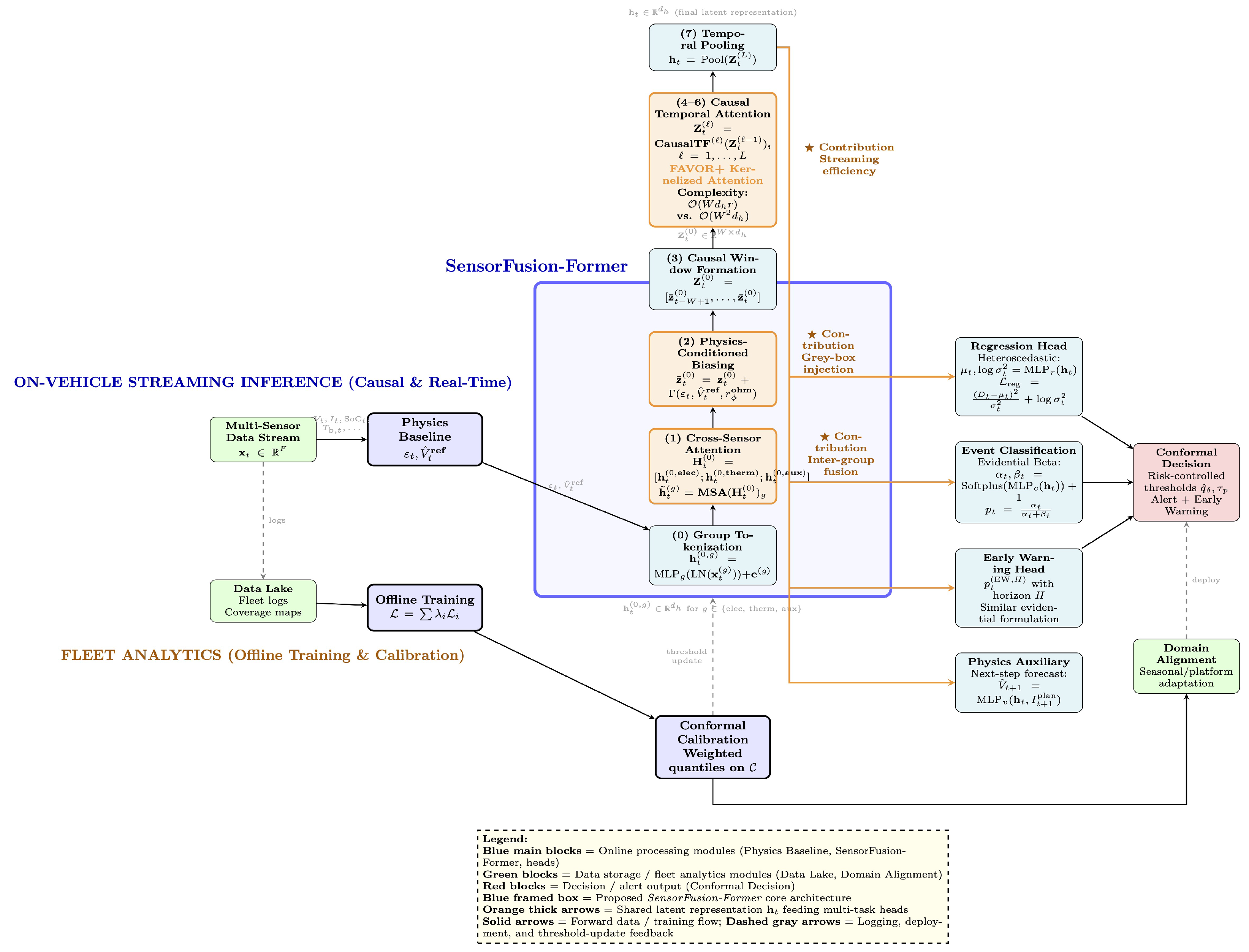
Figure 2.
Physics-guided voltage decomposition for operation-robust degradation detection. (a) Measured pack voltage and physics-guided reference across varying operating conditions. The shaded interval indicates a degradation episode with a sustained deviation from the healthy reference trajectory. (b) Operation-normalized residual remains small under benign operating variations and exceeds the threshold when degradation-related deviations occur. The early-warning interval precedes event onset by H samples.
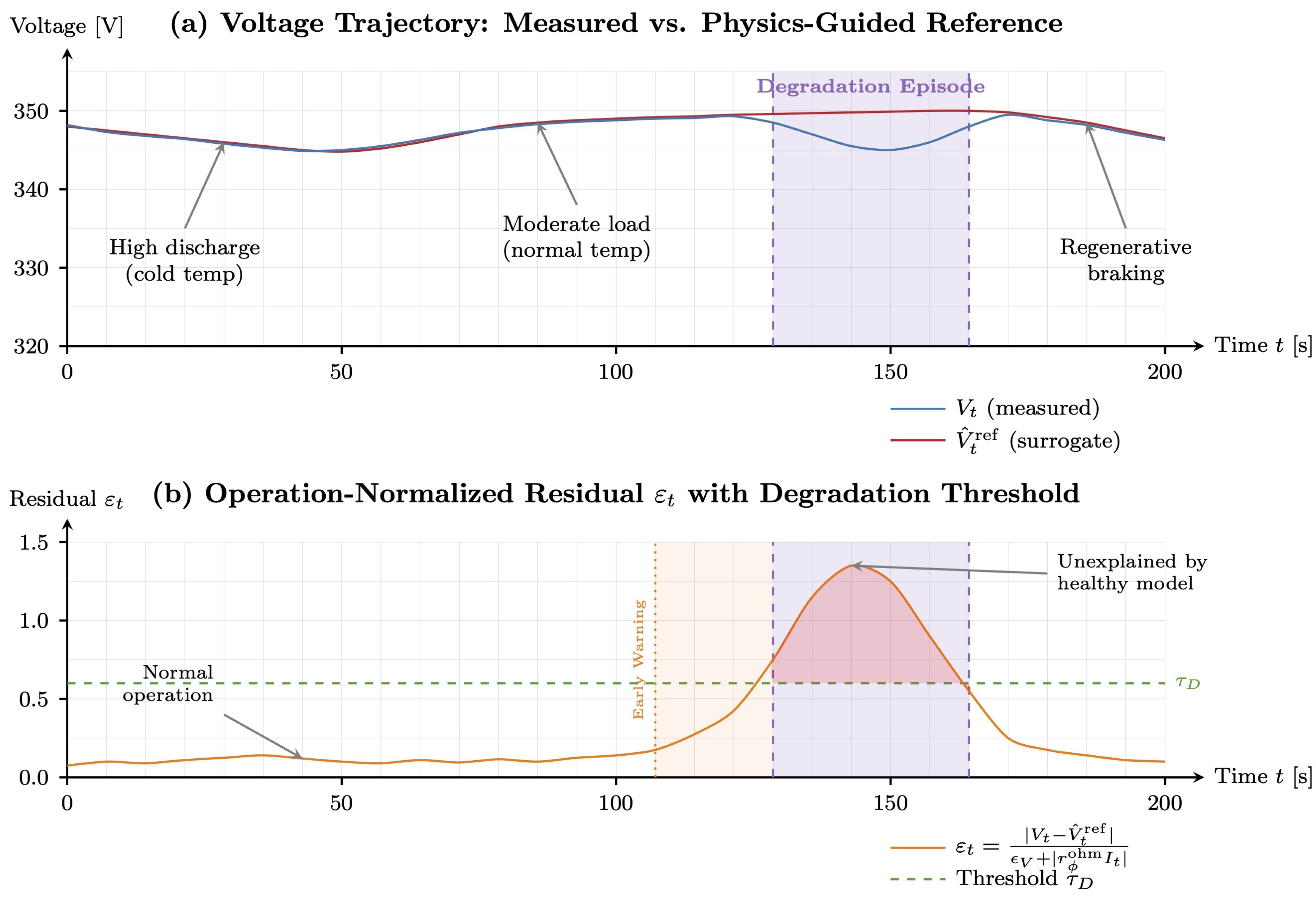
Figure 3.
Temporal smoothing pipeline for weak event label generation from physics-guided degradation signals. (a) Severity index computed from operation-normalized residuals with three peaks above the threshold . (b) Raw flags include isolated spikes, fragmented segments, and a short-lived transient. (c) Hysteresis filtering with suppresses isolated spikes while preserving sustained excursions. (d) Minimum-duration filtering with removes short segments that do not reflect sustained degradation. (e) Gap merging with consolidates segments separated by short gaps. (f) Final event label and the early-warning window that precedes event onset by samples.
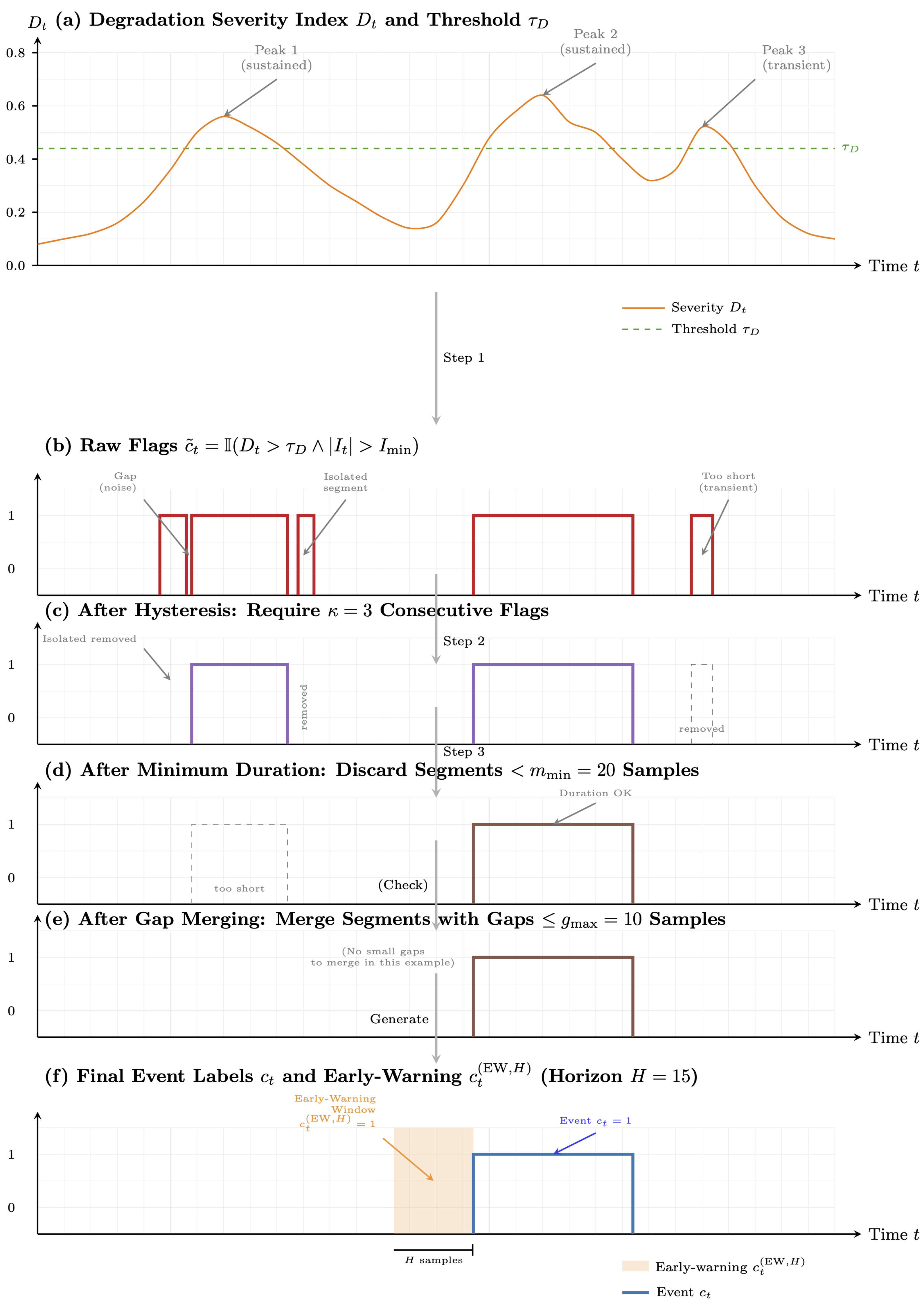
Figure 4.
Complete methodology pipeline from raw sensor data to deployment. The proposed framework follows a four-phase workflow: (1) physics-guided baseline training using healthy data, (2) weak label generation through operation-normalized residual analysis and temporal smoothing, (3) SensorFusion-Former training with unified multi-task objectives, and (4) weighted conformal calibration for risk-controlled deployment. The red dashed feedback loop indicates post-deployment domain adaptation using fleet-scale data. Color coding denotes functional roles: green boxes represent data acquisition and preprocessing, blue boxes indicate physics-guided modeling, orange boxes correspond to deep learning training, and red boxes denote deployment and decision-making components. Diamond-shaped nodes represent decision logic such as threshold checks and duration constraints.
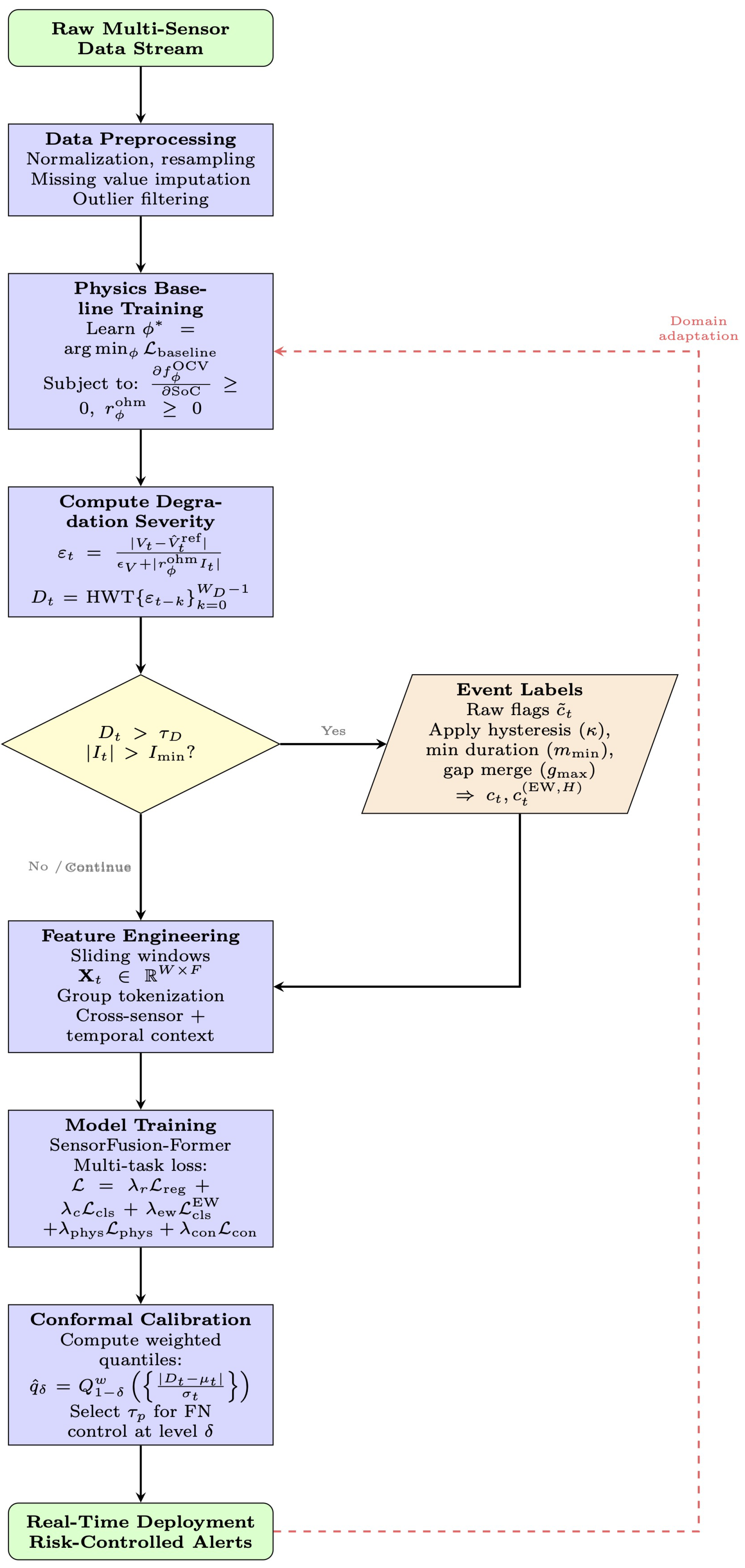
Figure 5.
Trade-off among F1 score, early-warning lead time, and FAR in Experiment 1.
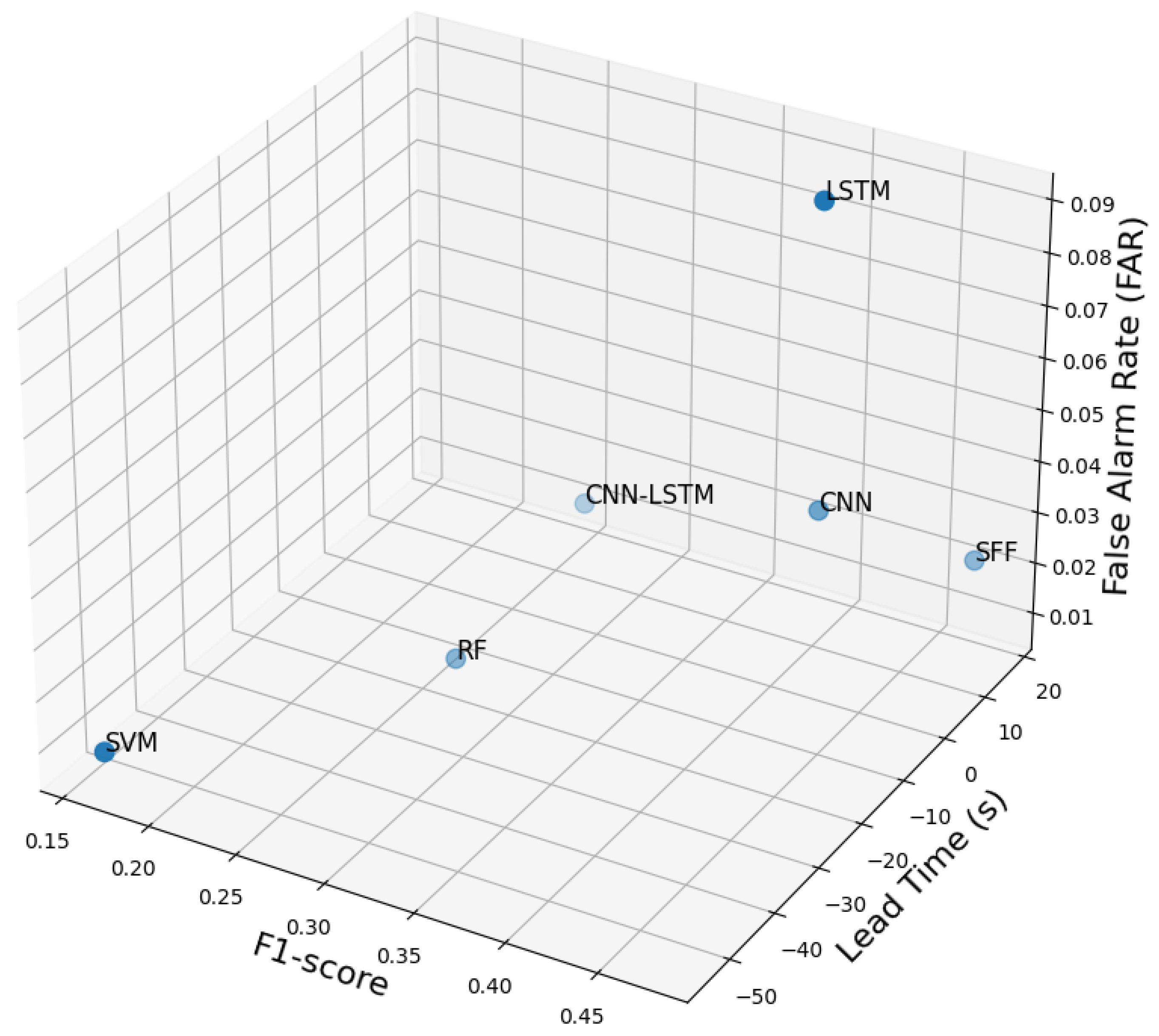
Figure 6.
Multi-metric ablation results for Experiment 2. Bars report AUROC, AUPRC, and F1, and the dashed curve reports ECE. The full SFF model achieves a strong balance between discriminative performance and calibration reliability, while removing key physics-guided or risk-control components degrades deployment-relevant behavior.
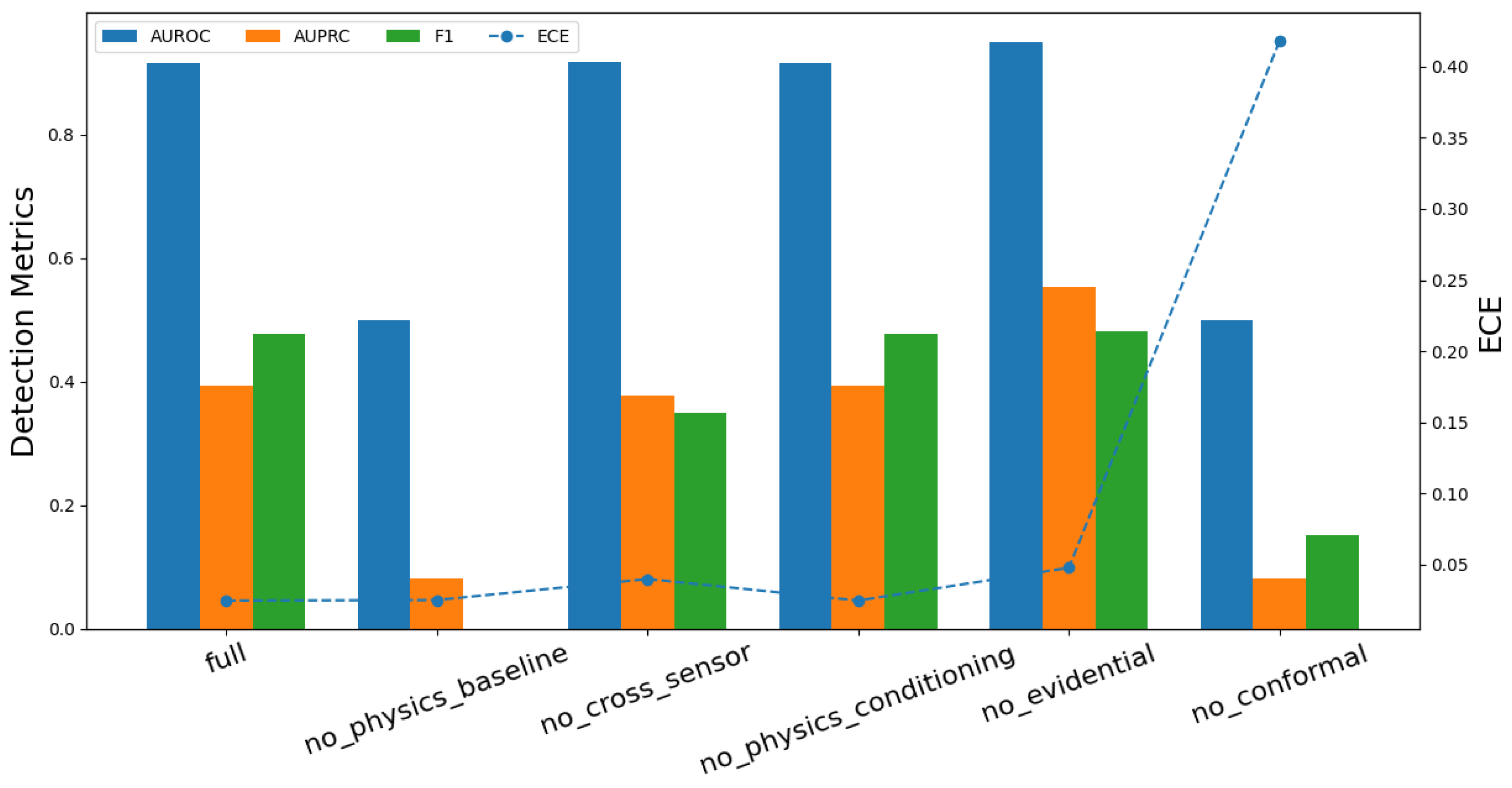
Figure 7.
Experiment 2 ablation study: three-dimensional trade-off among F1 score, FAR, and ECE. Each point corresponds to one model variant. The full model and the variant without physics conditioning are annotated below the markers, and the remaining ablated variants are annotated above the markers.
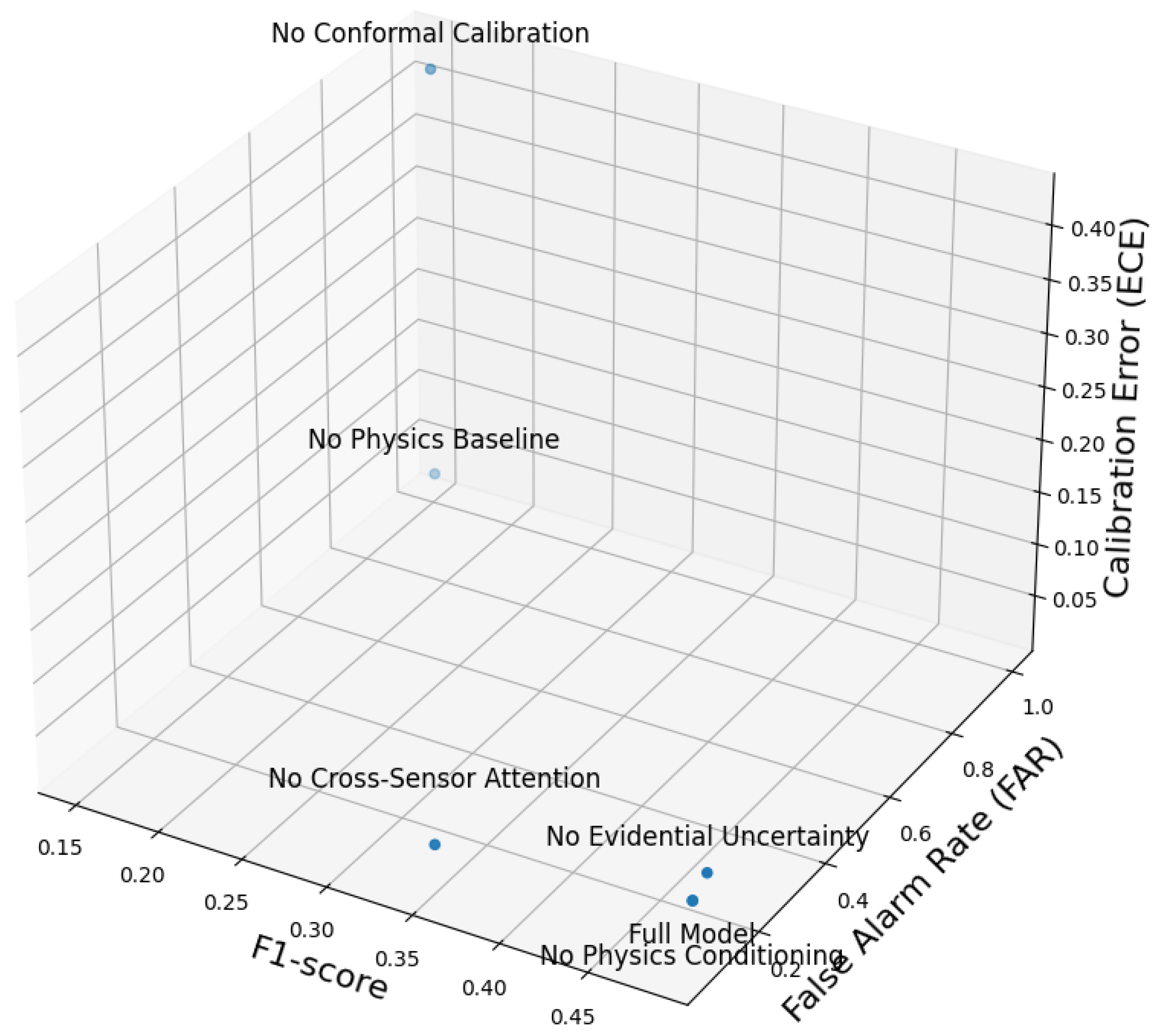
Figure 8.
Frame-level performance of SFF across three thermal scenarios in Experiment 3.
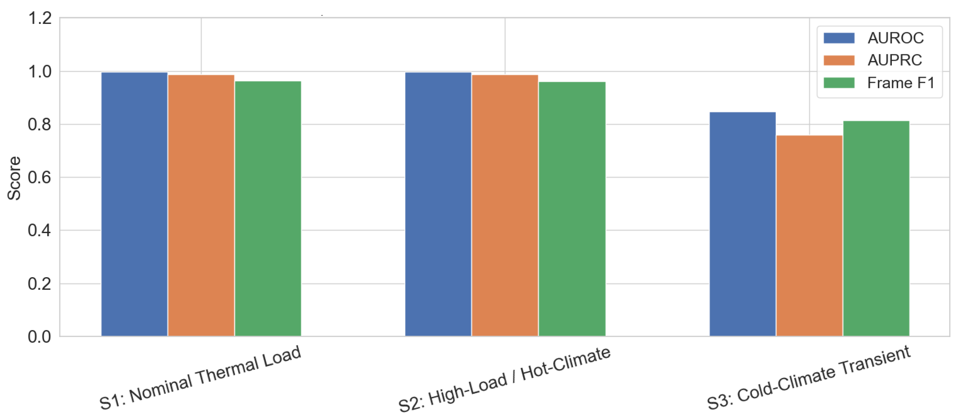
Figure 9.
Receiver operating characteristic (ROC) curves of SFF across the three thermal scenarios in Experiment 3. The diagonal line corresponds to random performance.
Figure 9.
Receiver operating characteristic (ROC) curves of SFF across the three thermal scenarios in Experiment 3. The diagonal line corresponds to random performance.
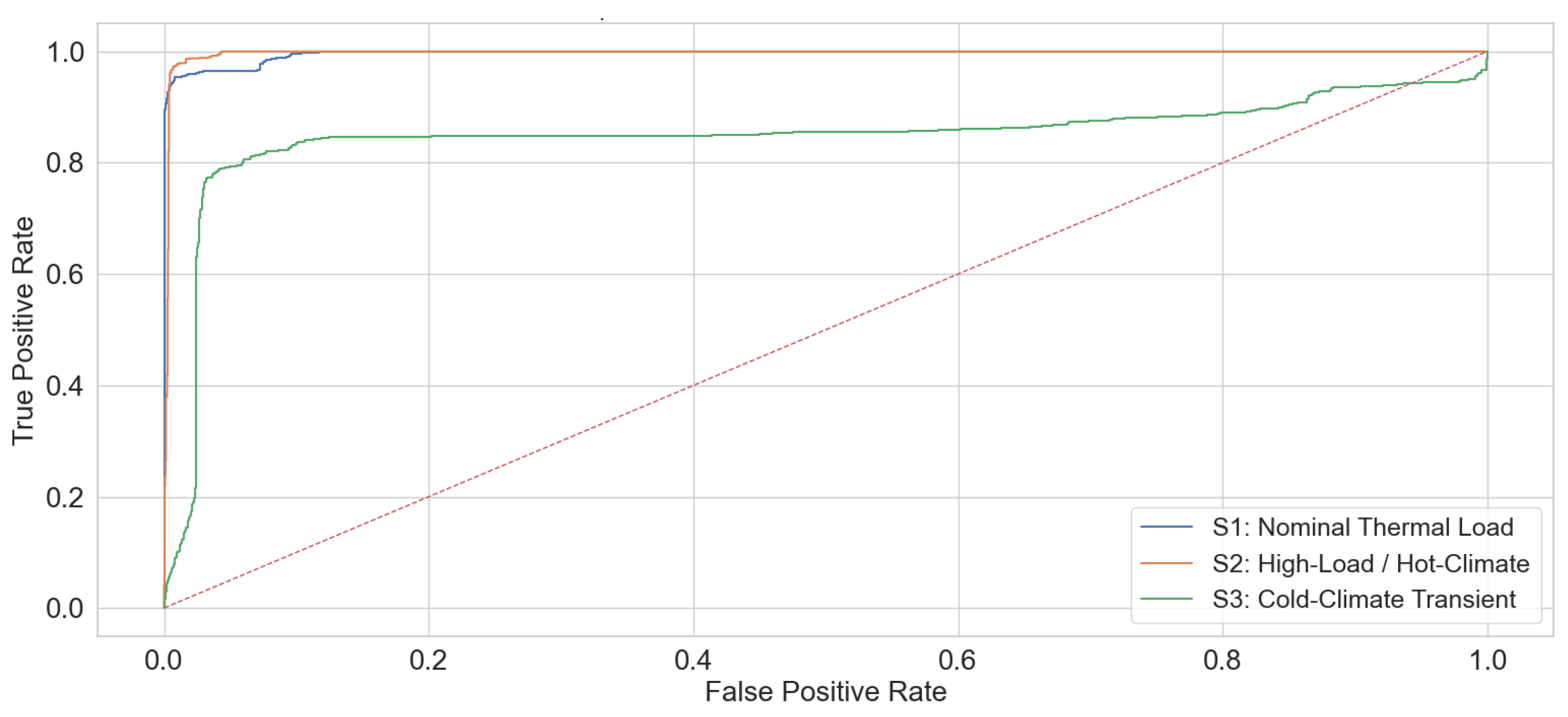
Figure 10.
Precision–recall (PR) curves of SFF across the three thermal scenarios in Experiment 3. PR curves highlight performance under class imbalance.
Figure 10.
Precision–recall (PR) curves of SFF across the three thermal scenarios in Experiment 3. PR curves highlight performance under class imbalance.
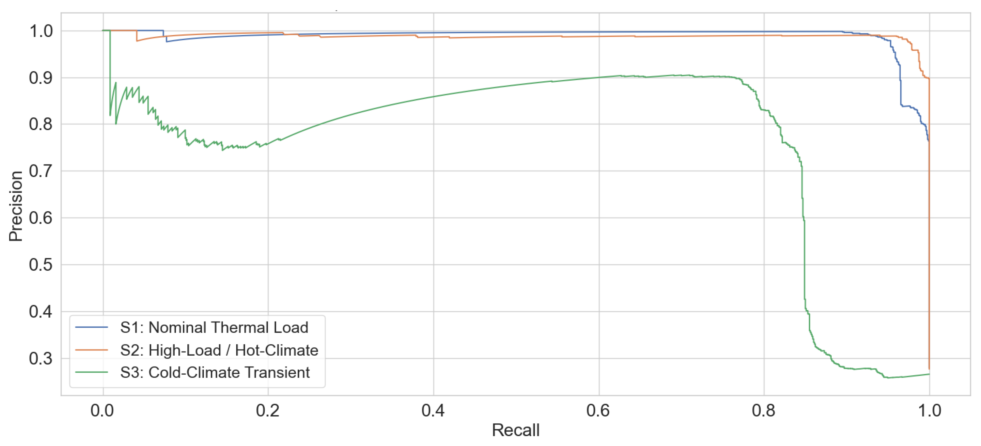
Figure 11.
Early-warning performance heatmaps for Experiment 4. (a) Warning Success Rate (WSR) across models and prediction horizons. (b) Mean lead time for successful warnings across the same settings.
Figure 11.
Early-warning performance heatmaps for Experiment 4. (a) Warning Success Rate (WSR) across models and prediction horizons. (b) Mean lead time for successful warnings across the same settings.
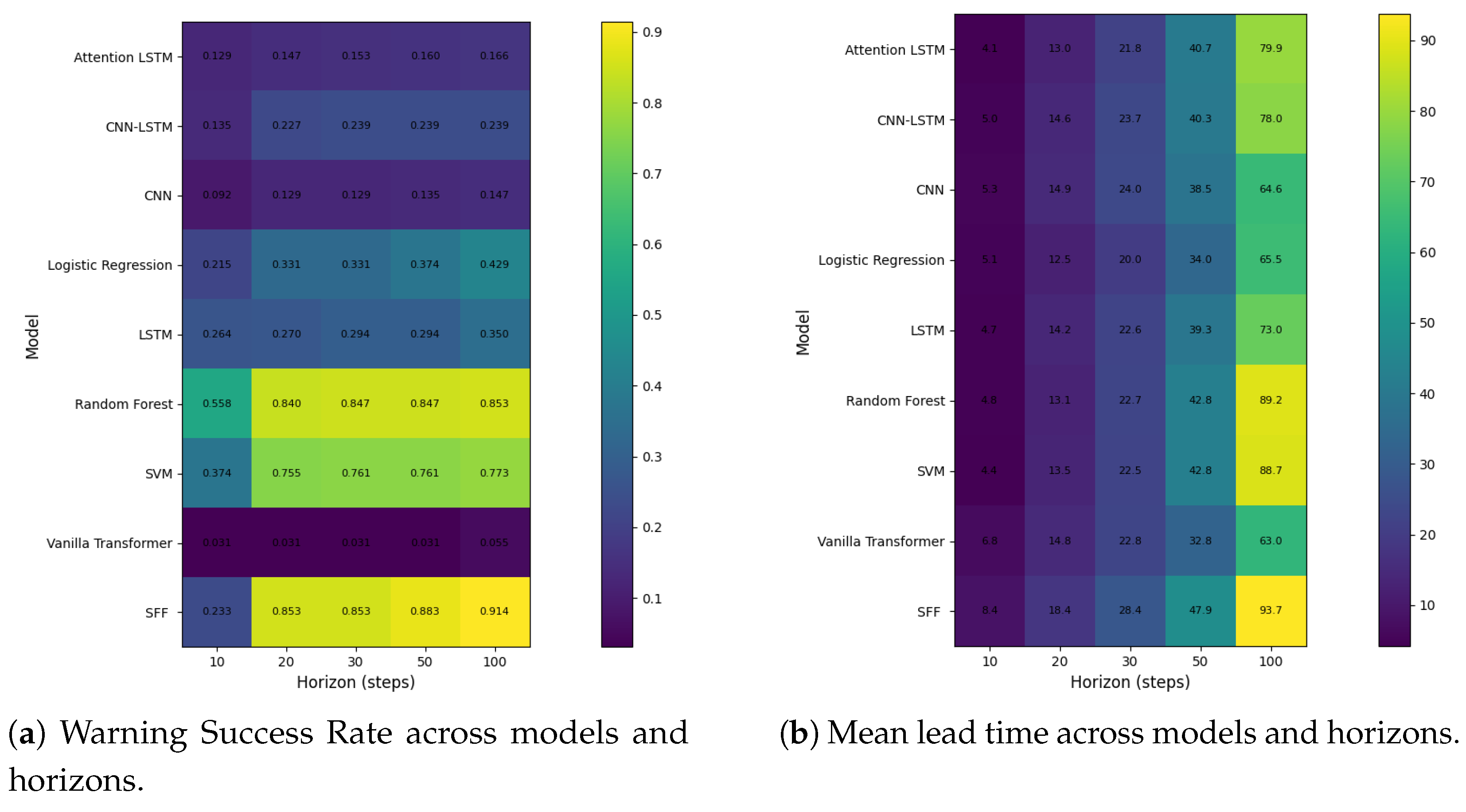
Figure 12.
Three-dimensional comparison of early-warning performance across prediction horizon, warning success rate, and lead time. The SFF trajectory exhibits a favorable balance between reliability and timeliness across all horizons.
Figure 12.
Three-dimensional comparison of early-warning performance across prediction horizon, warning success rate, and lead time. The SFF trajectory exhibits a favorable balance between reliability and timeliness across all horizons.
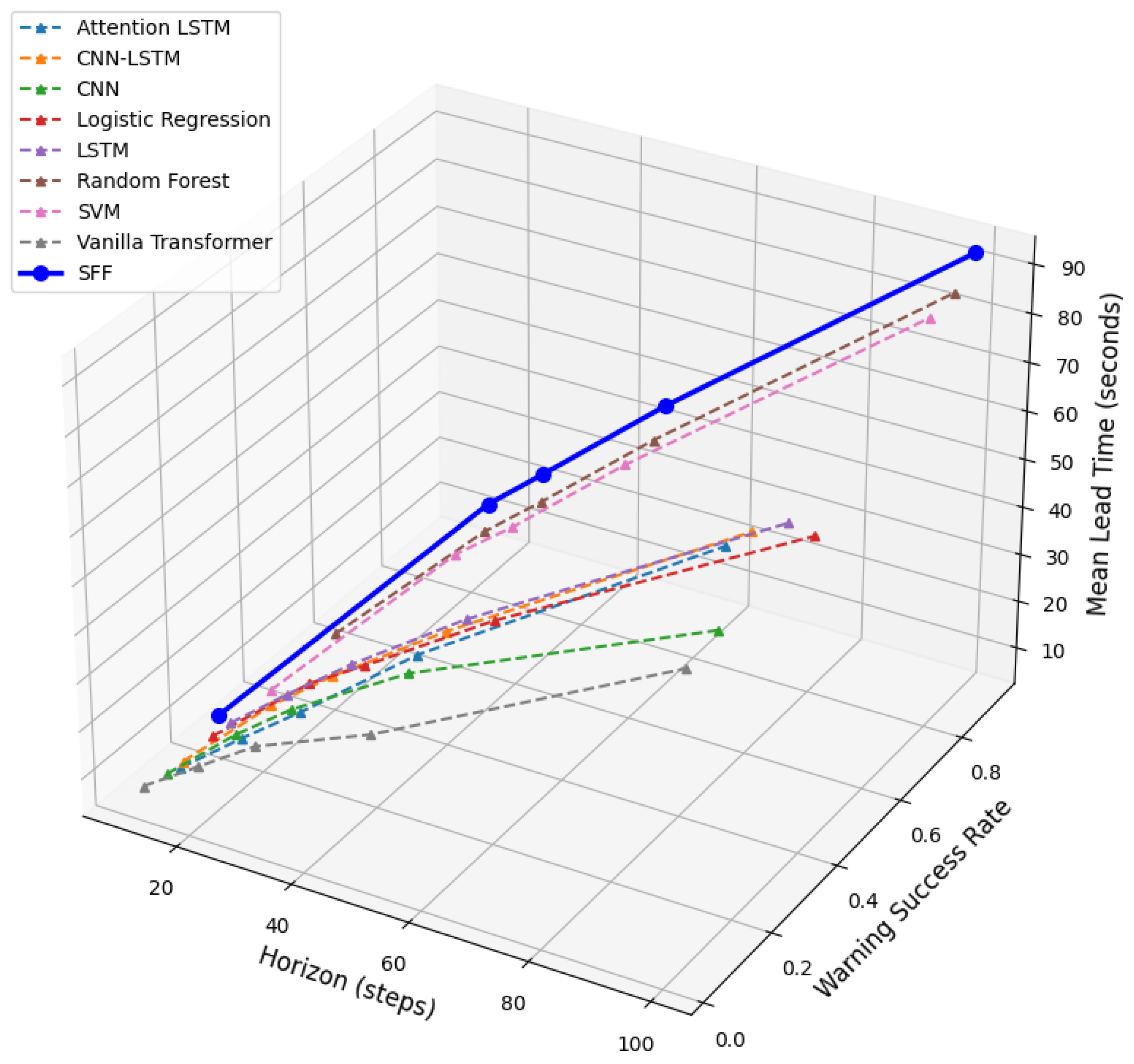

Table 1.
Key Symbols and Definitions Used in the System Model.
| Symbol | Description |
|---|---|
| Multi-sensor input vector at time t (electrical, thermal, auxiliary) | |
| Battery terminal voltage, current, and state-of-charge | |
| Physics-guided reference voltage under healthy operation | |
| Operation-normalized voltage residual indicating unexplained deviation | |
| Windowed degradation severity index derived from | |
| Binary event label indicating detected degradation | |
| Early-warning label for events occurring within horizon H | |
| Latent representation produced by the SensorFusion-Former | |
| Parameters of the physics-guided baseline voltage model | |
| Conformal quantile and probability threshold for risk-controlled decisions |
Table 2.
Computational Complexity of Representative Temporal Attention Mechanisms.
| Attention Type | Time Complexity | Memory |
|---|---|---|
| Vanilla Self-Attention | ||
| Reformer [50] | ||
| Linformer [51] | ||
| Linear Transformer [52] | ||
| FAVOR+ (ours) [49] | ||
| W: window length; : hidden dimension; r: FAVOR+ rank; k: projection dimension. | ||
| Example setting (, , ): FAVOR+ reduces attention cost from quadratic to linear in W. | ||
Table 3.
Overall Performance Comparison of Baseline Models and the Proposed SFF in Experiment 1.
| Method | AUC-ROC | AUC-PR | EDR | FAR | Lead Time (s) | Inf. Time (ms) |
|---|---|---|---|---|---|---|
| LR | 0.7676 | 0.2804 | 0.0000 | 0.0064 | – | 0.0012 |
| SVM | 0.7818 | 0.2504 | 0.0000 | 0.0085 | -54.0000 | 0.0298 |
| CNN-only | 0.8928 | 0.4265 | 0.1500 | 0.0339 | 6.0000 | 22.1320 |
| LSTM-only | 0.8716 | 0.3397 | 0.1500 | 0.0890 | 10.3333 | 24.4718 |
| CNN–LSTM | 0.8694 | 0.3526 | 0.1500 | 0.0254 | 2.6667 | 22.4190 |
| Vanilla TF | 0.8677 | 0.3636 | 0.0000 | 0.0000 | – | 21.9816 |
| SFF (Proposed) | 0.9118 | 0.4074 | 0.1500 | 0.0222 | 16.6667 | 6.7181 |
Table 4.
Ablation Study Results on TripB Corpus (Experiment 2).
| Variant | AUC-ROC | ROC | AUC-PR | PR | F1 | F1 | FAR | ECE |
|---|---|---|---|---|---|---|---|---|
| Full Model | 0.9155 | – | 0.3939 | – | 0.4768 | – | 0.1547 | 0.0244 |
| No Physics Baseline | 0.5000 | -0.4155 | 0.0817 | -0.3122 | 0.1511 | -0.3257 | 1.0000 | 0.0248 |
| No Cross-Sensor Attention | 0.9179 | +0.0025 | 0.3773 | -0.0166 | 0.3488 | -0.1280 | 0.0614 | 0.0396 |
| No Physics Conditioning | 0.9155 | +0.0000 | 0.3939 | +0.0000 | 0.4768 | +0.0000 | 0.1547 | 0.0244 |
| No Evidential Uncertainty | 0.9491 | +0.0336 | 0.5526 | +0.1588 | 0.4815 | +0.0047 | 0.1716 | 0.0475 |
| No Conformal Calibration | 0.5000 | -0.4155 | 0.0817 | -0.3122 | 0.1511 | -0.3257 | 1.0000 | 0.4183 |
Table 5.
Cross-Scenario Generalization Performance of SFF (Experiment 3).
| Scenario | AUROC | F1 | Lead Time (s) |
|---|---|---|---|
| S1: Nominal thermal load | 0.996 | 0.964 | 38.25 |
| S2: High-load, hot-climate | 0.997 | 0.960 | 42.75 |
| S3: Cold-climate transient | 0.848 | 0.814 | 50.00 |
Disclaimer/Publisher’s Note: The statements, opinions and data contained in all publications are solely those of the individual author(s) and contributor(s) and not of MDPI and/or the editor(s). MDPI and/or the editor(s) disclaim responsibility for any injury to people or property resulting from any ideas, methods, instructions or products referred to in the content. |
© 2026 by the authors. Licensee MDPI, Basel, Switzerland. This article is an open access article distributed under the terms and conditions of the Creative Commons Attribution (CC BY) license (http://creativecommons.org/licenses/by/4.0/).
Copyright: This open access article is published under a Creative Commons CC BY 4.0 license, which permit the free download, distribution, and reuse, provided that the author and preprint are cited in any reuse.


