
Submitted:
01 October 2025
Posted:
02 October 2025
You are already at the latest version
Abstract
Lithium-ion batteries play a key role in electric vehicles, so it is essential to continuously monitor and control their health. However, since today's battery packs are composed of hundreds or thousands of cells, monitoring them all continuously is challenging. Additionally, the performance of the entire battery pack is often limited by the weakest cell. Therefore, developing effective monitoring techniques to reliably forecast the remaining time to depletion (RTD) of lithium-ion battery cells is essential for safe and efficient battery management. However, even in robust systems, this data can be lost due to electromagnetic interference, microcontroller malfunction, failed contacts, and other issues. Gaps in voltage measurements compromise the accuracy of data-driven forecasts. This work systematically evaluates how different voltage reconstruction methods affect the performance of recurrent neural network (RNN) forecasters that are trained to predict RTD through quantile regression. The paper uses experimental battery pack data based on the behavior of an electric vehicle under dynamic driving conditions. Artificial gaps of 500 seconds were introduced at the beginning, middle, and end of each discharge phase, resulting in over 4300 reconstruction cases. Four reconstruction strategies were considered: a zero-order hold (ZOH), an autoregressive integrated moving average (ARIMA) model, a gated recurrent unit (GRU) model, and a hybrid unscented Kalman filter (UKF) model. The reconstructed signals were fed into LSTM and GRU RNNs to estimate RTD, which produced confidence intervals and median values for decision-making purposes.
Keywords:
lithium-ion batteries
; battery pack
; electric mobility
; dynamic load
; machine learning
; time-series forecast
; data reconstruction
1. Introduction
The accelerated deployment of lithium-ion (Li-ion) batteries in electric vehicles (EVs) and energy storage systems (ESS) is supported by their superior electrochemical performance, including high gravimetric and volumetric energy density, increased cycle life, and declining production costs [1,2] These characteristics position Li-ion batteries as the backbone of modern electrification and grid-integration initiatives. However, in the case of EVs, the dynamic operating conditions due to driving profiles, which involve rapid acceleration, regenerative braking, and load fluctuations, introduce significant complexity to monitoring and prediction tasks. Reliable estimation of the remaining discharge time under such conditions is critical, not only for accurate range forecasting required by the end-user, but also for ensuring robust battery management strategies by computers inside the vehicle. Advanced machine learning methods, such as recurrent neural networks (RNNs), have the potential to address the nonlinear and temporal dependencies of battery discharge dynamics. However, even with correct training, they depend on real-time data to provide a forecast.
A parallel challenge in real-world battery management lies in the incomplete availability of sensor data [3]. Failures in cell voltage sensors, intermittent communication losses, or bandwidth constraints can lead to temporary or persistent data gaps. These missing measurements compromise the accuracy of state estimation algorithms, which undermines the safety and performance of critical functionalities within the battery management system (BMS). For instance, voltage gaps may delay anomaly detection, reduce balancing efficiency, or introduce uncertainty into discharge time predictions during high-stress operating phases.
In the field of electric mobility, manufacturers use various communication and data-flow architectures for their battery systems. Each architecture has its own design trade-offs regarding scalability, modularity, latency, and redundancy. Nevertheless, every EV and plug-in hybrid electric vehicle (PHEV) requires the integration of a battery management system (BMS) [4,5]. A BMS is essential for ensuring safe operation, optimizing battery performance, and meeting regulatory and safety standards [6]. There are two primary architectural styles for implementing a BMS: a centralized BMS that integrates sensing, decision-making, and control functions, or a distributed master–slave configuration with multiple local BMS modules (slaves) communicating with a supervisory master node [7]. Either way, the system processes a large amount of sensor data in real time (see Figure 1), including individual cell voltages, currents, temperatures, and diagnostic signals [8]. However, the reliability of this data infrastructure is vulnerable to faults [9]. Sensor drift, connector degradation, electromagnetic interference, cable breaks, and microcontroller failures can generate communication or sensing gaps. When one or more data streams go missing or become invalid, the BMS may experience data gaps or corrupt inputs. These are highly undesirable due to the importance of the battery in vehicle operation [10]. Voltage is particularly critical because it defines safe operational limits and is directly tied to overvoltage/undervoltage cutoff mechanisms. Any cell voltage deviation beyond prescribed thresholds can result in degradation, imbalance, or catastrophic failure [11].
However, the challenge extends beyond simply filling gaps. In practice, missing data may be correlated with fault conditions rather than random events. If reconstruction models assume randomness, they may mask incipient failures and delay corrective measures. For this reason, anomaly-aware reconstruction strategies that explicitly model uncertainty and interface with diagnostic systems are critical for ensuring safety in fault-prone environments [12,13]. Bringing together advanced reconstruction strategies and distributed learning architectures can elevate the reliability and safety of EV and ESS operation beyond current baselines. This approach not only addresses the technical limitations of sensor infrastructure but also supports broader objectives, such as reducing range anxiety, optimizing lifecycle costs, and enabling secure integration with renewable-heavy power grids.
There is a wide range of reconstruction techniques, from statistical interpolation to data-driven methods that exploit correlations among neighboring cells or modules. The choice of reconstruction strategy directly affects the quality of the model's inputs and, consequently, the reliability of the downstream prediction [14]. Nevertheless, few studies have examined how different reconstruction approaches influence RNN forecasting under dynamic load profiles.
RNNs are well-suited for modeling complex, nonlinear time-series signals because they are designed to process sequential data while retaining memory of past inputs [15]. Unlike traditional feedforward networks, RNNs maintain a hidden state that evolves over time. This allows RNNs to learn temporal dependencies and internal dynamics that are not directly observable [16]. This makes them especially powerful for applications like battery modeling, in which voltage and current signals may exhibit nonlinear behavior due to electrochemical hysteresis, load variability, or multi-timescale dynamics. By capturing the sequential structure of these signals, RNNs can accurately predict future values or reconstruct missing data, even in the presence of noise and variability.
This paper addresses that gap by benchmarking multiple reconstruction methods in the context of RTD prediction. RTD is defined as the time interval until a cell branch reaches its cutoff voltage under a dynamic drive cycle. It is a relevant metric for range estimation and discharge scheduling. Our analysis evaluates the ability of different reconstruction techniques to recover realistic input signals and maintain RNN predictive accuracy using representative driving cycles characterized by rapid current transients and partial data unavailability. The findings provide insights into the coupled roles of data recovery and sequence modeling, providing a more resilient and accurate battery management in next-generation EVs and energy storage systems.
2. Materials and Methods
The methodology proposed in this work follows a two-stage approach. First, artificial gaps are systematically introduced into the experimental battery cycling data at various points within the discharge profile. Then, these missing segments are reconstructed using various reconstruction techniques. Both the reconstructed signals and the original signal are retained for analysis. Second, the reconstructed voltage trajectories serve as inputs for recurrent neural network models that were previously trained to forecast the remaining time to depletion. This combined process enables evaluation of the direct accuracy of each reconstruction strategy and its effect on forecasting performance, providing an integrated view of how data recovery choices influence predictive reliability.
Figure 2 illustrates the methodology applied in this research.
2.1. Analyzed Reconstruction Methods
This paper compares four reconstruction strategies with increasing levels of complexity: the zero-order hold (ZOH), autoregressive integrated moving average (ARIMA), unscented Kalman filter (UKF), and gated recurrent unit (GRU), a type of RNN. While these methods have different requirements, they are all evaluated over the same gap regions of driving cycle data to ensure comparability.
The first and the simplest method, is the ZOH, which propagates the last valid value across the gap [17]. It is computationally inexpensive and easy to implement since it does not depend on any other parameters. For voltage reconstruction, the estimated voltage at the gap from the last known voltage v at time k with m missing samples is calculated as follows,
The ARIMA is a classical statistical forecasting model used for time-dependent variables [18]. ARIMA assumes that present voltage is shaped by its history, corrections from past prediction errors, and long-term differences. This makes ARIMA suitable for analyzing signals where past electrical states influence the present [19]. ARIMA can be expanded to consider seasonal information. It consists of three main components: the integrated part d, the autoregressive component p, and the moving average order q.
In (2), is the -th differenced version of the voltage time series , which is differenced until it becomes stationary. is the lag (backshift) operator that shifts the values backward in time. In (3), the coefficient scales the contribution of a past value of the differenced voltage through the autoregressive component: The random error has a zero mean and constant variance. The coefficient scales the influence of a past error through the moving average component.
No predefined models were used. Instead, a custom Python script was used to preprocess the data and leverage the auto_arima procedure from the pmdarima Python package [20], which automatically calculates the best model orders (p,d,q) by minimizing the fitting error. The resulting ARIMA model was then used to recursively forecast and fill the voltage gap.
The third approach investigated for data reconstruction is the Unscented Kalman Filter (UKF). The UKF results by applying the unscented transformation to the Kalman filter framework [21]. It models a nonlinear, discrete-time system defined by the state transition function and the measurement function as [22],
In (4), captures the system dynamics and nonlinearities, represents auxiliary inputs, is the absolute timestamp, denotes process noise, maps the system state to the measurement space, and represents measurement noise. A hybrid state-transition model is introduced that incorporates information from neighboring cells in the battery pack, as well as a predictive model derived from past data of the target cell as,
where is the average of available auxiliary cell values, defines the coupling strength, and ρ, which is within the range [0,1], balances the contribution of the predictive model against the auxiliary cell term. The predictive model is expressed as follows,
The parameters a, b, c, d and e are estimated fitting historical data from earlier cycles and the period before the missing region. Thus, the model combines logarithmic terms to capture boundary behavior and uses a quadratic polynomial to describe nonlinear trends across flatter regions. For the observation model, a direct observation is used as follows,
which implies that the measurements directly observe the internal state, subject to Gaussian noise with a zero mean and a covariance R. During missing intervals, however, no actual measurements are available, so the UKF relies solely on the prediction step, without applying measurement updates.
The UKF advances the state vector , represented by the mean and the covariance , by constructing sigma points , which are representative samples of the state distribution,
The scaling parameter is defined as,
where controls the spread of the sigma points, and is a secondary scaling constant. Then, each sigma point is propagated through the nonlinear state function, which is expressed as follows,
Then, the predicted mean and the covariance P values are obtained as,
where is the process noise covariance, and and are the sigma points for the mean and covariance weights, respectively, which are calculated as follows,
Here, is an additional parameter, commonly set to 2 for Gaussian distributions, that increases the weight of the central sigma point. Finally, the process noise is approximated using prediction residuals as,
The fourth method considered is a recurrent neural network, specifically the gated recurrent unit (GRU). GRUs are a type of RNN designed to model sequential data and are well-suited for learning temporal dynamics in systems where measurements are strongly time-dependent. GRUs regulate the flow of information across time steps through their gating mechanisms, allowing the network to retain relevant history while reducing the vanishing gradient issues that typically limit the performance of conventional RNNs. This makes GRUs particularly effective at capturing the nonlinear, time-varying behavior of electrochemical processes during battery discharge.
In this implementation, the model uses a fixed lookback window of about 2 minutes to predict the subsequent voltage point. Each input sequence incorporates terminal voltage, current, state of charge (SoC), and elapsed time. This provides the network with complementary information about the evolving system state. The architecture consists of an input layer that handles the feature vector, two stacked GRU layers with 252 hidden units each, and a fully connected output layer that produces a single scalar prediction of the reconstructed voltage. The network weights were initialized randomly before training, enabling the optimizer to discover suitable representations of the system dynamics from scratch. Since voltage appears in both the input and output, the model can operate in an autoregressive manner, recursively using its own predictions. However, stability across reconstruction gaps is maintained through the use of exogenous inputs, such as current and elapsed time.
Figure 3 describes the architecture employed for implementing the GRU.
Training was conducted using the AdamW optimizer with weight decay regularization and early stopping to prevent overfitting and memorization. Convergence was achieved with a root mean squared error (RMSE) of 10 mV on the training dataset. This target was not arbitrary; it was selected to align with the requirements of practical BMSs for balancing, ensuring that the reconstruction accuracy is directly relevant to operational decision-making.
Three key performance indicators were used to evaluate the performance of the proposed reconstruction methods and establish a benchmark for comparison: the root mean square error (RMSE), the mean absolute error (MAE), and the coefficient of determination (R2). These metrics are formally defined as follows,
where is the actual voltage value, is the predicted voltage, is the mean of the actual values and n is the number of observations.
2.2. Analyzed RTD Forecasting Methods
The forecasting objective is to estimate the remaining time to depletion (RTD), which is defined as the time interval until the cell or branch voltage drops below the cutoff threshold, Voff. So if tcutoff is defined as the time instance at which V(t) = Voff, the RTD can be defined as,
Figure 4 shows the baseline calculation of the RTD at a specific time during a driving cycle (WLTP). Unlike static state variables, such as SoC, RTD is a dynamic variable whose value evolves as a function of the current operating profile, instantaneous load, and cell voltage response history. In practice, RTD provides a direct, interpretable measure of available operating time under real-world driving conditions, such as the WLTP.
Forecasting the RTD is challenging because input signals, such as cell voltages, branch currents, and elapsed time, exhibit strong nonlinear behavior. Under WLTP conditions, rapid current transients, rest periods, and voltage relaxation effects create complex temporal dependencies that simple regression approaches and curve-fitting techniques cannot capture. This work employs a RNN architecture to address these challenges, and two of the most common implementations are compared: the GRU and the LSTM networks.
An LSTM is a type of RNN that incorporates gating mechanisms and an internal cell state that acts as a memory line. This allows the network to retain information over longer time periods and makes LSTMs well-suited for modeling the long-term temporal dependencies present in real driving cycles
Both GRU and LSTM networks are advanced types of RNNs designed to capture long-range dependencies in sequential data and address the vanishing gradient problem. The key difference between the two lies in their internal structure. LSTMs use three gates (input, forget, and output) and maintain two states (cell and hidden), which allows them to control the flow of information more selectively. GRUs simplify this mechanism by using only two gates (reset and update) and a single hidden state. This makes GRUs computationally more efficient, yet they still achieve comparable performance on many sequence modeling tasks. GRUs tend to train faster and require fewer parameters. However, LSTMs may offer more flexibility for learning complex temporal patterns in longer sequences.
The proposed framework implements identical model architectures. The models are trained using historical sequences of current, voltage, and elapsed time, together with derived features such as power SoC within a 120-second lookback window. Rather than attempting to explicitly forecast full future current and voltage behavior, the network is optimized to estimate the RTD at each time step. This method transforms the problem into a supervised learning task, in which the target variable is the true remaining time until voltage cutoff, calculated from experimental data. Through these temporal correlations in the input features, the model learns to associate characteristic load-voltage- SoC patterns with the typical time remaining before depletion.
Additionally, both model networks express their output in terms of quantiles of the RTD distribution. This provides a point estimate (the median RTD) and an uncertainty band. This probabilistic formulation achieved through a pinball loss function [23,24] is particularly useful since it incorporates reliable confidence intervals which are essential for ensuring safe and efficient operation under uncertain or variable driving conditions. For this work, three quantile levels, defined as τ, were selected to achieve an 80% of confidence in the predictions. The selected quantile levels are, τ = 0.5 for the 50% quantile (median), τ = 0.1 for the 10% quantile and τ = 0.9 for the 90% quantile.
The pinball loss function Lτ used to train the RNN uses the ground of truth y and the model prediction . It is defined as,
Using equation (17), we can see that the loss function penalizes errors differently depending on whether the prediction is too low (underestimation) or too high (overestimation). For example, if the true RTD (y) is 1000 s and the model predicts = 800 s, the underestimation of 200 s generates only a minor penalty of 0.1 x 200 = 20. However, the same underestimation at = 800 s is penalized nine times more strongly, 0.9 x 200 = 180. On the contrary, if the model overestimates with = 1200 s, the penalty becomes 0.9 x 200 = 180, while the same overestimation with = 1200 s results in a penalty of only 0.1 x 200 = 20. This asymmetric weighting causes the lower quantile to remain below most outcomes, the upper quantile to stay above them, and the median quantile to balance both. Consequently, the three outputs collectively approximate the empirical distribution of RTD rather than generating a single point estimate. When this methodology is used to adjust the neuron weights inside the RNN, the model learns to satisfy all three loss functions simultaneously, providing a confidence range and a median value, for reference.
Figure 5 shows the RNN structure for the GRU and LSTM models, which have three quantile outputs.
Two aspects were considered to evaluate the validity of RNN predictions: the decreasing monotonicity of predicted quantile values and the prediction interval coverage probability (PICP).
Since the RNN is free to predict any values and the initial weights are randomly assigned, the decreasing monotonicity must be evaluated. Ensuring monotonicity confirms that the quantile curves do not cross each other. The rule for decreasing monotonicity is as follows,
Testing the PICP against the true RTD and the predicted values, , can ensure that the selected confidence interval is reliable, or reveal if it is overconfident (too narrow) or underconfident (too wide). The PICP for an 80% prediction interval is defined as the fraction of test instances in which the true RTD falls between and . This condition can be expressed as,
where n is the total number of time samples, yk is the ground of truth RTD at time instance k, and are the predicted 10th and 90th quantile values forecasted at time instance k.
We also define the width of the PICP as follows,
This is the width of the confidence interval of the RTD prediction expressed in seconds.
3. Dataset
The methodologies evaluated in this work rely on a dataset obtained with an advanced battery testbench that is specifically designed to reproduce realistic electric vehicle operating conditions [25]. While executing dynamic load profiles derived from the WLTP test cycle, the testbench supports independent monitoring of individual cell voltages, branch currents, and pack-level signals. The fully modular system architecture integrates with a BMS via CAN communication, enabling real-time exchange of voltage, current, state-of-charge, and diagnostic messages. This design allows laboratory cycling to closely replicate real automotive usage in terms of both electrical dynamics and data acquisition fidelity. A detailed description of the test bench hardware, data acquisition structure, and communication layers is provided in [26].
Figure 6 shows the electrical diagram of the testing setup and the acquired signals.
The test object is a lithium-ion battery pack made up of Panasonic NCR18650B cells. These cells are a commercially available 18650-format NCA chemistry. The nominal specifications of each cell are as follows,
- Chemistry: NCA
- Nominal capacity: 3.2 Ah
- Nominal voltage: 3.6 V
- Charge conditions: CC-CV at 0.5C (cut off at 65 mA or after 4 hours)
The cells were arranged in a 12-series by 3-parallel (S12P3) configuration. This resulted in a pack with a nominal voltage of 43.2 V and a total nominal capacity of approximately 9.6 Ah. This configuration provides sufficient energy to reproduce full WLTP driving cycles while maintaining observability at the cell and pack levels. This is essential for evaluating reconstruction methods under realistic load conditions. For the purposes of this study, only the driving cycles were used, as constant charge is more trivial to predict. To prevent data bias, the dataset was split into two segments. Specifically:
- Training set (40 driving cycles): used for training data-driven reconstruction methods such as GRUs, and for training the RNN models for RTD forecasting.
- Evaluation set (40 driving cycles): reserved exclusively for testing all reconstruction methods and assess their impact on RTD forecasting accuracy.
The evaluation set corresponds to the driving cycles numbered 249 through 350 in the dataset. This design ensures that the reported results reflect the methods' ability to generalize to unseen operating conditions rather than memorize specific trajectories.
Figure 7 shows an example of the voltage behavior of the battery pack under the tested driving conditions (WLTP).
4. Results
This section presents the study results in three parts. First, signals with missing data are reconstructed and the R2, RMSE, and MAE metrics are evaluated for each reconstruction method (see Figure 8a). Next, the designed RTD forecasting model is evaluated against the original signal using complete data (see Figure 8b). This evaluation relies on the mean MAE, as well as the coverage and width of the 80% prediction interval (PICP80%). Finally, the forecasting results obtained with each reconstructed dataset are presented and assessed using the same set of metrics (see Figure 8c). Together, these analyses allow us to evaluate individual reconstruction methods and their combined performance with the forecasting model.
Figure 8 summarizes the three parts of the results presented in this section.
4.1. Reconstruction Results
This section evaluates how well the ZOH, ARIMA, UKF, and GRU algorithms reconstruct missing data from the original signals (see Figure 8a).
To evaluate the performance of the reconstruction methods, independent tests were conducted across 36 cells of the battery pack over 40 cycles. Three 500-second artificial gaps were simulated at different positions within the discharge phase in each tested cycle, resulting in 4320 test cases. Then, each reconstruction method was applied to reconstruct the missing signal interval.
Figure 9 shows representative reconstruction results for cycle 315, focusing on cell S1P1 of the battery pack.
The average values of the performance metrics of the different evaluated reconstruction methods are summarized in Table 1.
The results clearly show differences in the effectiveness of the evaluated reconstruction methods. Both ARIMA and ZOH have negative average R2 values, indicating very poor predictive capability, while RMSE and MAE values remain relatively high and comparable to one another. In contrast, the GRU (RNN) achieves an average R2 of 0.79, with substantially lower RMSE and MAE values. This demonstrates its ability to effectively capture temporal dependencies due to its capability of handling more inputs. Finally, the UKF algorithm outperforms the other methods by achieving the highest R2 value (0.91) and the lowest RMSE and MAE values. This underscores its robustness for signal reconstruction in this context. This can be attributed to its knowledge of the state of neighboring cells and its ability to fit historic data.
4.2. RTD Forecast Based on the Original Signal of Past Data
This section evaluates the performance of the GRU and LSTM RNN models for RTD forecasting of the original signals of past data (see Figure 8b).
Because the designed RTD forecasting model produces probabilistic outputs, both the PICP80% and PICPwidth values must be assessed. In addition, the median estimate () is reported, because it is a meaningful indicator of model performance. The evaluation was conducted on 40 driving cycles distinct from those used in training across 36 cells. At each time step, the pre-trained models were applied. Since the RNN models were configured with a 120-second lookback window, estimations are only available from that point onward. Figure 10 illustrates an example, and Figure 11 shows the RTD forecast performance indicators based on the original signal of past data compared with the RTD of the complete original signal.
and the confidence band PICPwidth evaluated at each time step of the driving cycle.
corresponding to each evaluated RNN model. On the right, PICP80% coverage for each evaluated RNN model.
Table 2 summarizes the values of the performance indicators of the RTD forecast based on the original signal of past data when compared with the RTD of the complete original signal. The evaluation was conducted on 40 driving cycles distinct from those used in training across 36 cells.
As shown in Figure 11 and Table 2, the LSTM achieved lower median RTD error (MAE of 26.7 versus 28.6 s), higher PICP80% coverage (93.1% versus 88.2%), and a narrower PICPwidth (126.6 s versus 159.1 s) than the GRU across the 1440 WLTP evaluated discharge cycles. This indicates improved accuracy and better-calibrated uncertainty.
4.3. RTD Forecast Based on the Reconstructed Signal of Past Data
This section evaluates the performance of the GRU and LSTM RNN models for RTD forecasting of the reconstructed signals of past data (see Figure 8c). To ensure comparability, the evaluation was conducted using the same cycles and injected gaps as in previous sections. This yielded 4320 test cases for each reconstruction method and RTD forecasting model. Figure 12 and Figure 13 show box plots of the GRU and LSTM forecasting results, respectively, based on all analyzed reconstruction methods. A complete summary of the performance indicators is provided in Table 3.
corresponding to each evaluated RNN model. On the right, PICP80% coverage for each evaluated GRU model.
corresponding to each evaluated RNN model. On the right, PICP80% coverage for each evaluated LSTM model.
As expected, the performance of both the GRU and LSTM models for RTD forecasting decreased when evaluated with reconstructed time series. These results highlight two points. First, introducing reconstruction noise inevitably degrades performance compared to the complete original data. Second, the LSTM forecaster is superior because it combines high accuracy with reliable uncertainty estimates.
When artificial gaps were introduced and filled using different reconstruction methods, the UKF consistently minimized the degradation, providing forecasts similar to the original past data signal. GRU-based reconstruction was the second-best method, but it doubled the errors. Simpler reconstruction methods, such as ZOH and ARIMA, substantially degraded accuracy, with ARIMA producing the poorest MAE values despite showing PCIP80% and PCIPwidth values similar to those of the better methods.
The relationship between MAE and PCIPwidth requires further analysis. For most combinations, the PCIPwidth values were larger than the MAE values. For example, the LSTM+UKF combination had PCIPwidth = 126 s bands and MAE = 38 s, indicating that the true RTD generally fell within the confidence interval. This trade-off is acceptable because it ensures reliability, even if it means broader ranges. However, the opposite occurred in ARIMA-reconstructed cases, where the MAE values exceeded the PCIPwidth values (e.g., LSTM+ARIMA with MAE = 153.5 s and PCIPwidth = 121.4 s). This reflects an overconfident model response, meaning that the [,] interval is too narrow relative to the actual error. This explains the reduced PCIP80% values observed.
5. Conclusions
A Battery Management System (BMS) processes a large volume of data, and the electric powertrain operates under demanding conditions. These factors make system components, such as sensors and cables, prone to temporary malfunctions or permanent failures. These issues can lead to missing or corrupted signals, which directly impact the reliability of sensing data and consequently affect the decision-making of critical subsystems in electric vehicles. Robust methods are required to address data gaps and maintain continuity in system monitoring to ensure safe and reliable operation.
This paper has evaluated several techniques for reconstructing missing data, including zero-order hold (ZOH), the unscented Kalman filter (UKF), the autoregressive integrated moving average (ARIMA) model, and a recurrent neural network based on gated recurrent units (GRUs). In addition to reconstruction, we evaluated the reconstructed signals by using them as inputs for two time-to-depletion (RTD) forecasting models. This two-step evaluation allows to assess the performance of the reconstruction methods based not only on their accuracy but also on their usefulness in forecasting tasks.
The results demonstrate that the UKF provides the most reliable signal reconstruction, outperforming traditional statistical approaches and learning-based methods. In terms of forecasting, the LSTM model performs slightly better than the GRU model. The hybrid approach combining UKF-based reconstruction and LSTM-based forecasting yields the best overall results, surpassing all other combinations tested. These findings are validated using data collected from a controlled test bench designed to replicate realistic driving conditions, demonstrating the practical relevance of the proposed methodology for real-world electric vehicle applications.
Author Contributions
Conceptualization, J.d.l.V., J.-R.R., and J.A.O.-R.; methodology, J.A.O.-R.; software, J.d.l.V. and J.-R.R.; validation, J.d.l.V., J.-R.R., and J.A.O.-R.; formal analysis, J.-R.R. and J.A.O.-R.; investigation, J.d.l.V., J.-R.R., and J.A.O.-R.; resources, J.-R.R. and J.A.O.-R.; data curation, J.d.l.V.; writing—original draft preparation, J.d.l.V. and J.-R.R.; writing—review and editing, J.d.l.V., J.-R.R., and J.A.O.-R.; supervision, J.-R.R. and J.A.O.-R. All authors have read and agreed to the published version of the manuscript.
Funding
This project received funding from grant TED2021-130007B-I00, by MICIU/AEI/10.13039/501100011033/ and by ERDF “A way of making Europe,” by the European Union and from the Agència de Gestió d’Ajuts Universitaris i de Recerca-AGAUR (2021 SGR 00392).
Institutional Review Board Statement
Not applicable.
Informed Consent Statement
Not applicable.
Data Availability Statement
The data used in this manuscript is available in the public repository “Lithium-ion battery pack cycling dataset with CC-CV charging and WLTP/constant discharge profiles” located at https://dataverse.csuc.cat/dataset.xhtml?persistentId=doi:10.34810/data2395.
Conflicts of Interest
The authors declare no conflict of interest.
References
- Ostadi, A.; Kazerani, M.; Chen, S. K. Optimal sizing of the Energy Storage System (ESS) in a Battery-Electric Vehicle. 2013 IEEE Transp. Electrif. Conf. Expo Components, Syst. Power Electron. - From Technol. to Bus. Public Policy, ITEC 2013 2013.
- Kumar, R.R.; Bharatiraja, C.; Udhayakumar, K.; Devakirubakaran, S.; Sekar, K.S.; Mihet-Popa, L. Advances in Batteries, Battery Modeling, Battery Management System, Battery Thermal Management, SOC, SOH, and Charge/Discharge Characteristics in EV Applications. IEEE Access 2023, 11, 105761–105809. [CrossRef]
- Xiong, R.; Yu, Q.; Shen, W.; Lin, C.; Sun, F. A Sensor Fault Diagnosis Method for a Lithium-Ion Battery Pack in Electric Vehicles. IEEE Trans. Power Electron. 2019, 34, 9709–9718. [CrossRef]
- Spoorthi, B.; Pradeepa, P. Review on Battery Management System in EV. 2022 Int. Conf. Intell. Controll. Comput. Smart Power, ICICCSP 2022 2022.
- Prada, E.; Di Domenico, D.; Creff, Y.; Sauvant-Moynot, V. Towards advanced BMS algorithms development for (P)HEV and EV by use of a physics-based model of Li-ion battery systems. World Electr. Veh. J. 2013, 6, 807–818. [CrossRef]
- Li, B.; Fu, Y.; Shang, S.; Li, Z.; Zhao, J.; Wang, B. Research on Functional Safety of Battery Management System (BMS) for Electric Vehicles. Proc. - 2021 Int. Conf. Intell. Comput. Autom. Appl. ICAA 2021 2021, 267–270.
- Popp, A.; Fechtner, H.; Schmuelling, B.; Kremzow-Tennie, S.; Scholz, T.; Pautzke, F. Battery Management Systems Topologies: Applications: Implications of different voltage levels. 2021 IEEE 4th Int. Conf. Power Energy Appl. ICPEA 2021 2021, 43–50.
- Khan, F.I.; Hossain, M.; Lu, G. Sensing-based monitoring systems for electric vehicle battery – A review. Meas. Energy 2025, 6. [CrossRef]
- Kosuru Rahul, V. S.; Kavasseri Venkitaraman, A. A Smart Battery Management System for Electric Vehicles Using Deep Learning-Based Sensor Fault Detection. World Electr. Veh. J. 2023, Vol. 14, Page 101 2023, 14, 101.
- Li, J.; Che, Y.; Zhang, K.; Liu, H.; Zhuang, Y.; Liu, C.; Hu, X. Efficient battery fault monitoring in electric vehicles: Advancing from detection to quantification. Energy 2024, 313. [CrossRef]
- Jeevarajan, J.A.; Joshi, T.; Parhizi, M.; Rauhala, T.; Juarez-Robles, D. Battery Hazards for Large Energy Storage Systems. ACS Energy Lett. 2022, 7, 2725–2733. [CrossRef]
- Haider, S.N.; Zhao, Q.; Li, X. Data driven battery anomaly detection based on shape based clustering for the data centers class. J. Energy Storage 2020, 29. [CrossRef]
- Bhaskar, K.; Kumar, A.; Bunce, J.; Pressman, J.; Burkell, N.; Rahn, C.D. Data-Driven Thermal Anomaly Detection in Large Battery Packs. Batteries 2023, 9, 70. [CrossRef]
- Liu, J.; He, L.; Zhang, Q.; Xie, Y.; Li, G. Real-world cross-battery state of charge prediction in electric vehicles with machine learning: Data quality analysis, data repair and training data reconstruction. Energy 2025, 335. [CrossRef]
- Sherstinsky, A., Fundamentals of Recurrent Neural Network (RNN) and Long Short-Term Memory (LSTM) Network. Phys. D Nonlinear Phenom. 2020, 404, 132306.
- Saha, P.; Dash, S.; Mukhopadhyay, S. Physics-incorporated convolutional recurrent neural networks for source identification and forecasting of dynamical systems. Neural Networks 2021, 144, 359–371. [CrossRef]
- Karafyllis, I.; Krstic, M. Nonlinear Stabilization Under Sampled and Delayed Measurements, and With Inputs Subject to Delay and Zero-Order Hold. IEEE Trans. Autom. Control. 2011, 57, 1141–1154. [CrossRef]
- Zhou, Y.; Huang, M. Lithium-ion batteries remaining useful life prediction based on a mixture of empirical mode decomposition and ARIMA model. Microelectron. Reliab. 2016, 65, 265–273. [CrossRef]
- Riba, J.-R.; Gómez-Pau, Á.; Martínez, J.; Moreno-Eguilaz, M. On-Line Remaining Useful Life Estimation of Power Connectors Focused on Predictive Maintenance. Sensors 2021, 21, 3739. [CrossRef]
- pmdarima: ARIMA estimators for Python — pmdarima 2.0.4 documentation https://alkaline-ml.com/pmdarima/ (accessed Sep 29, 2025).
- He, Z.; Dong, C.; Pan, C.; Long, C.; Wang, S. State of charge estimation of power Li-ion batteries using a hybrid estimation algorithm based on UKF. Electrochim. Acta 2016, 211, 101–109.
- Xiong, K.; Zhang, H.; Chan, C. Performance evaluation of UKF-based nonlinear filtering. Automatica 2006, 42, 261–270. [CrossRef]
- Liu, S.; Deng, J.; Yuan, J.; Li, W.; Li, X.; Xu, J.; Zhang, S.; Wu, J.; Wang, Y.-G. Probabilistic quantile multiple fourier feature network for lake temperature forecasting: incorporating pinball loss for uncertainty estimation. Earth Sci. Informatics 2024, 17, 5135–5148. [CrossRef]
- Bauer, I.; Haupt, H.; Linner, S. Pinball boosting of regression quantiles. Comput. Stat. Data Anal. 2024, 200. [CrossRef]
- de la Vega Hernández, J.; Ortega Redondo, J. A.; Riba Ruiz, J.-R. Lithium-ion battery pack cycling dataset with CC-CV charging and WLTP/constant discharge profiles; CORA.Repositori de Dades de Recerca, 2025.
- de La Vega, J.; Riba, J.-R.; Ortega, J. A. Advanced Battery Test Bench For Realistic Vehicle Driving Conditions Assessment; Institute of Electrical and Electronics Engineers Inc., 2025; pp. 1–6.
Figure 1.
Sensor in a central BMS architecture.
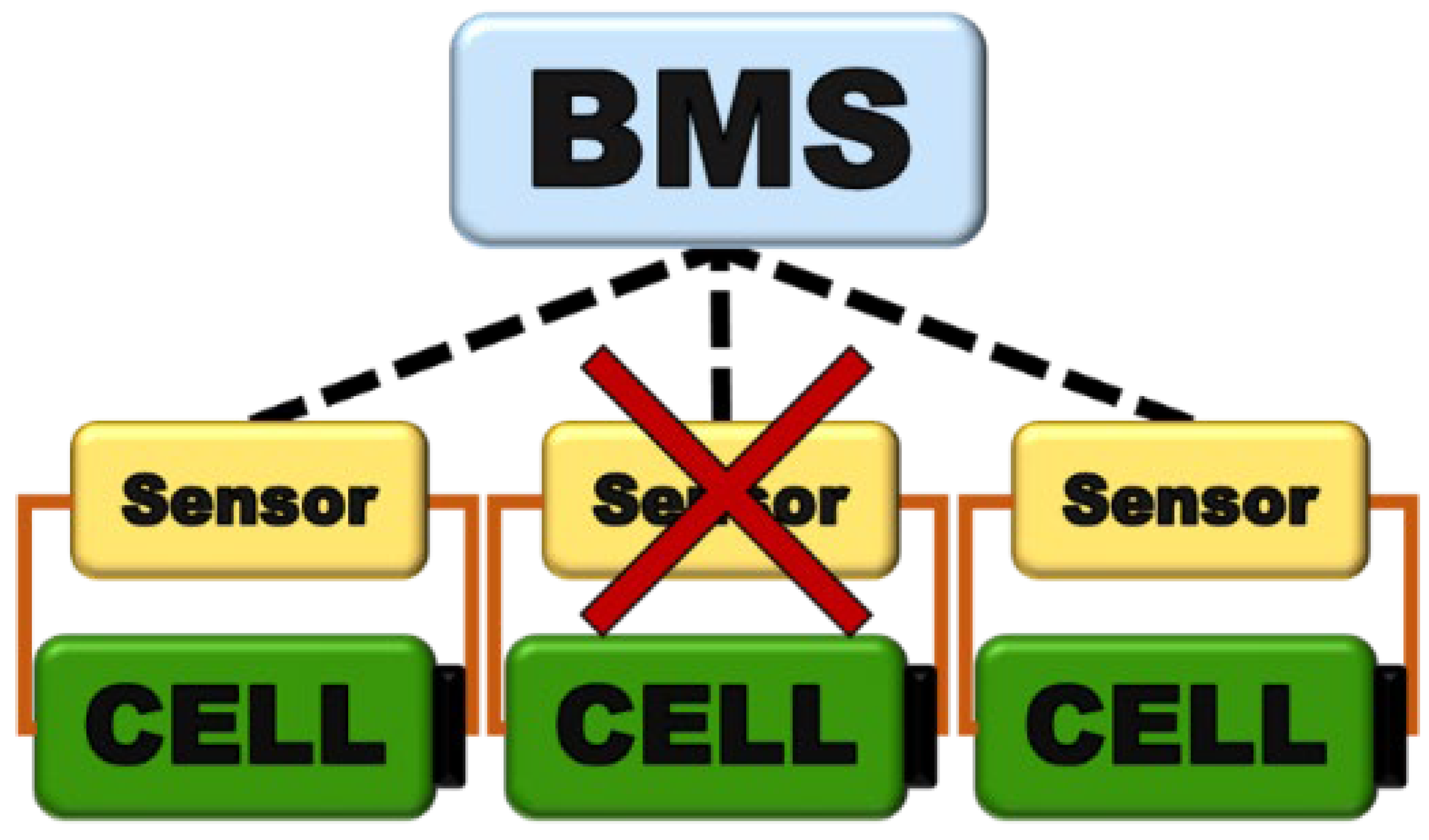
Figure 2.
Reconstruction and RTD forecast evaluation methodology.
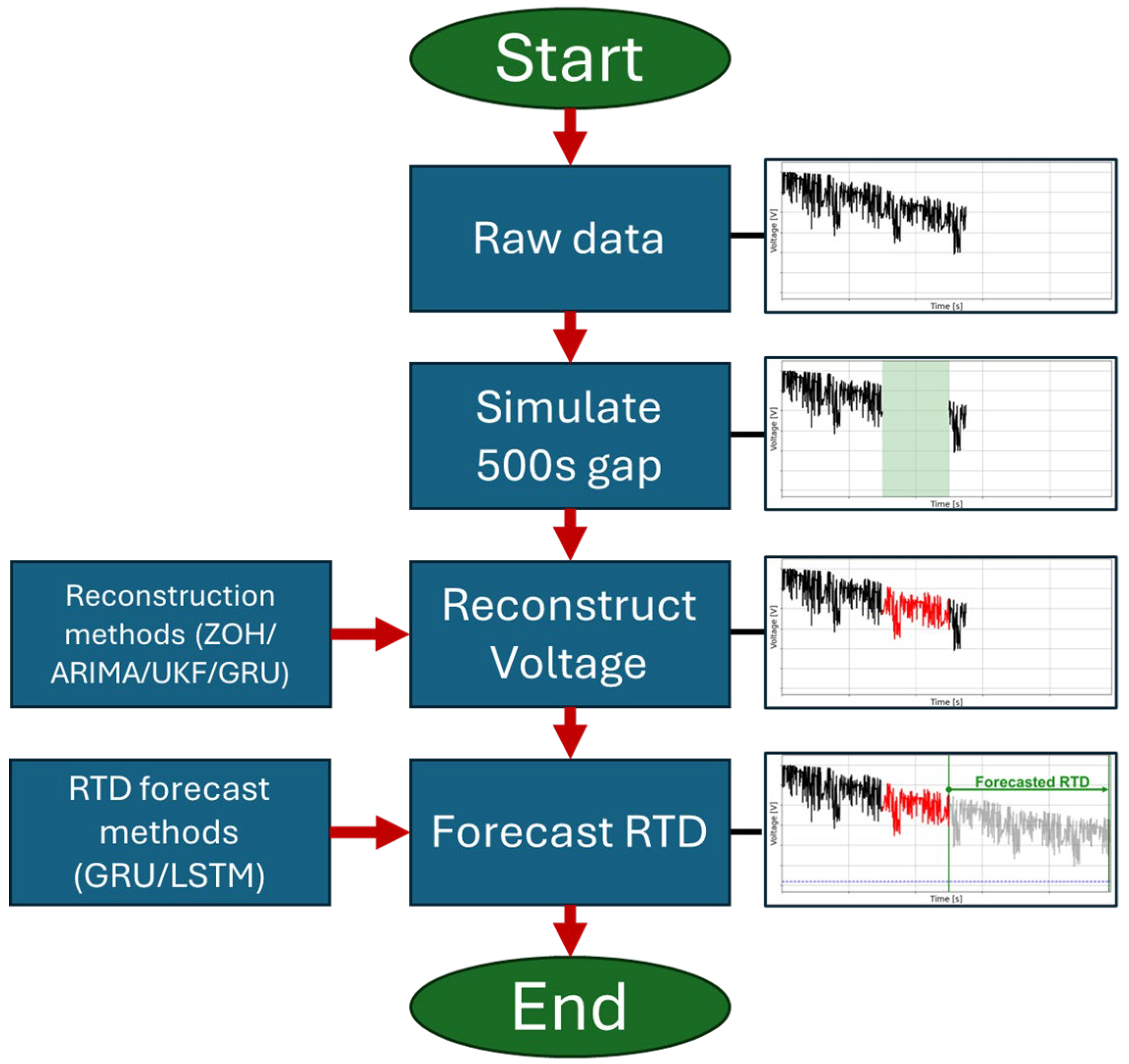
Figure 3.
GRU-RNN architecture reconstruction.
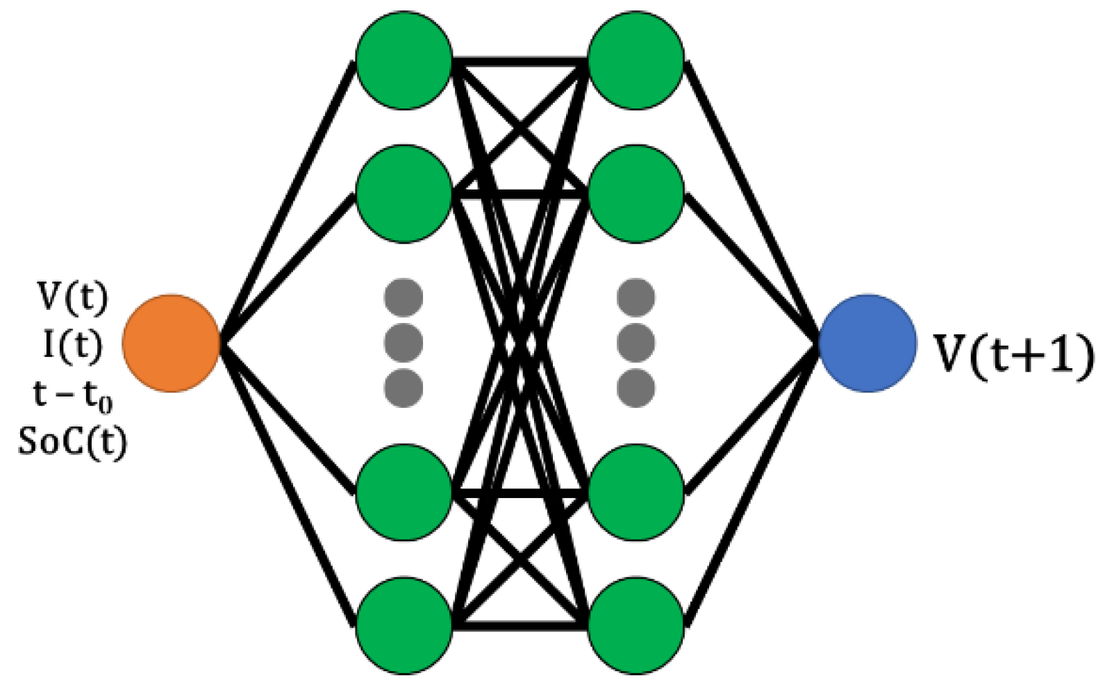
Figure 4.
Remaining time for depletion measurement.
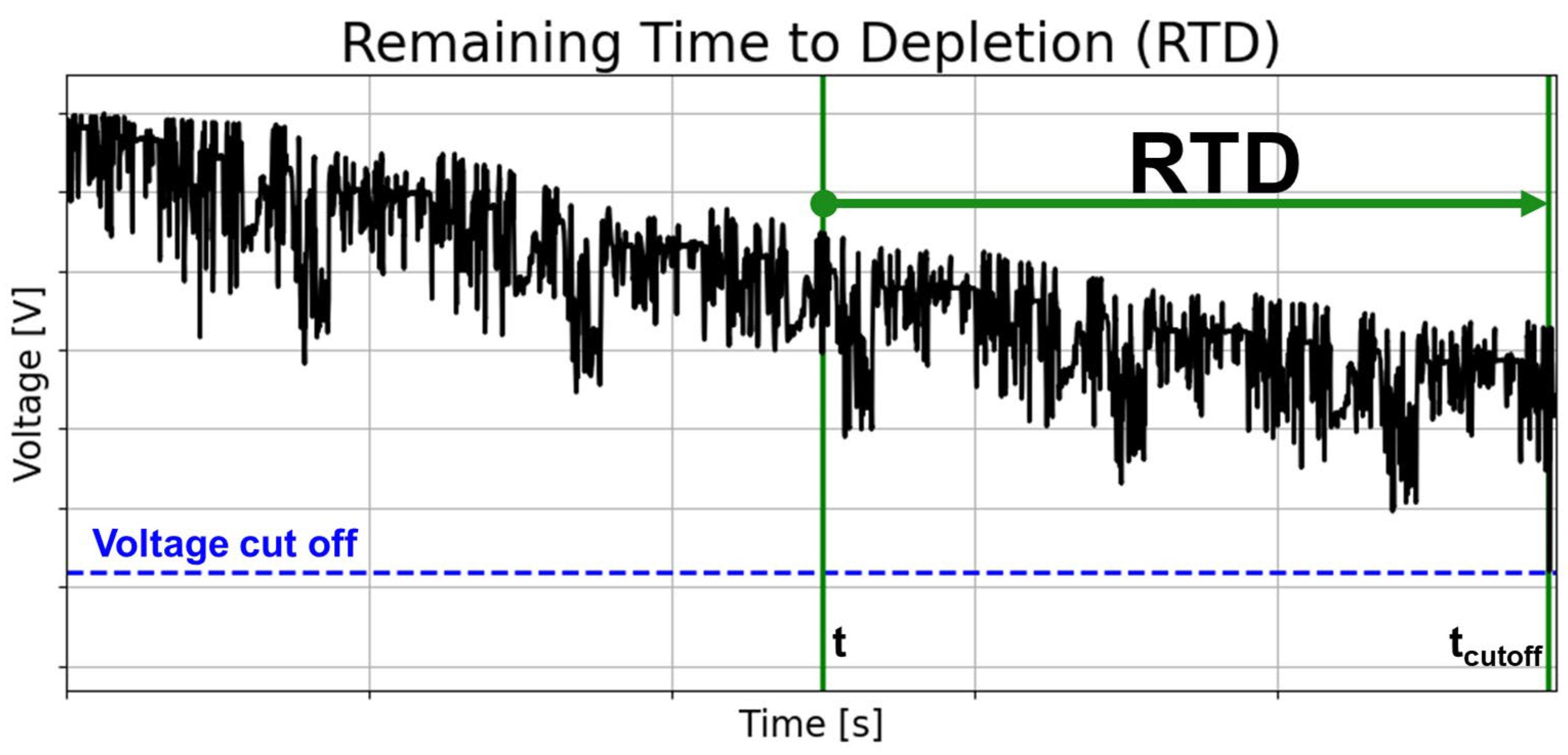
Figure 5.
GRU and LSTM model architectures for RTD forecasting.
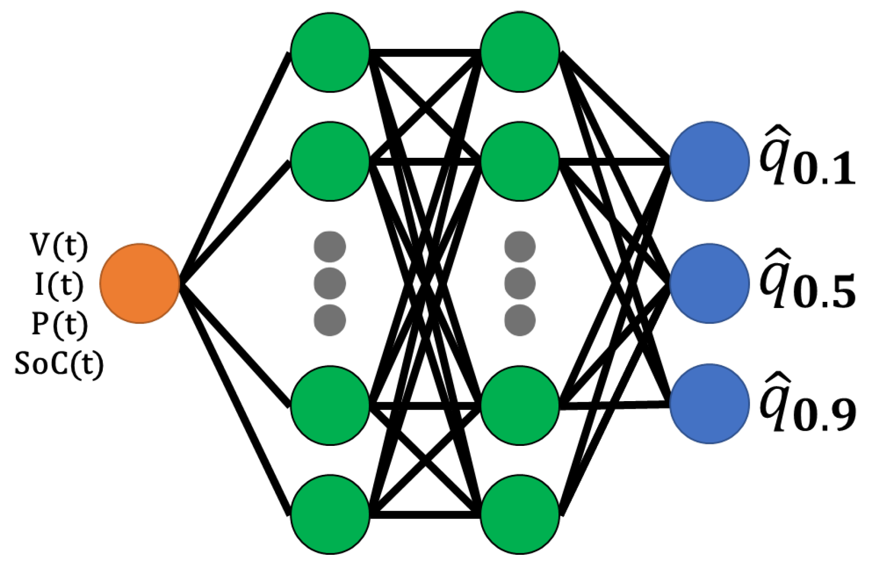
Figure 6.
Electrical diagram of the battery testing setup.
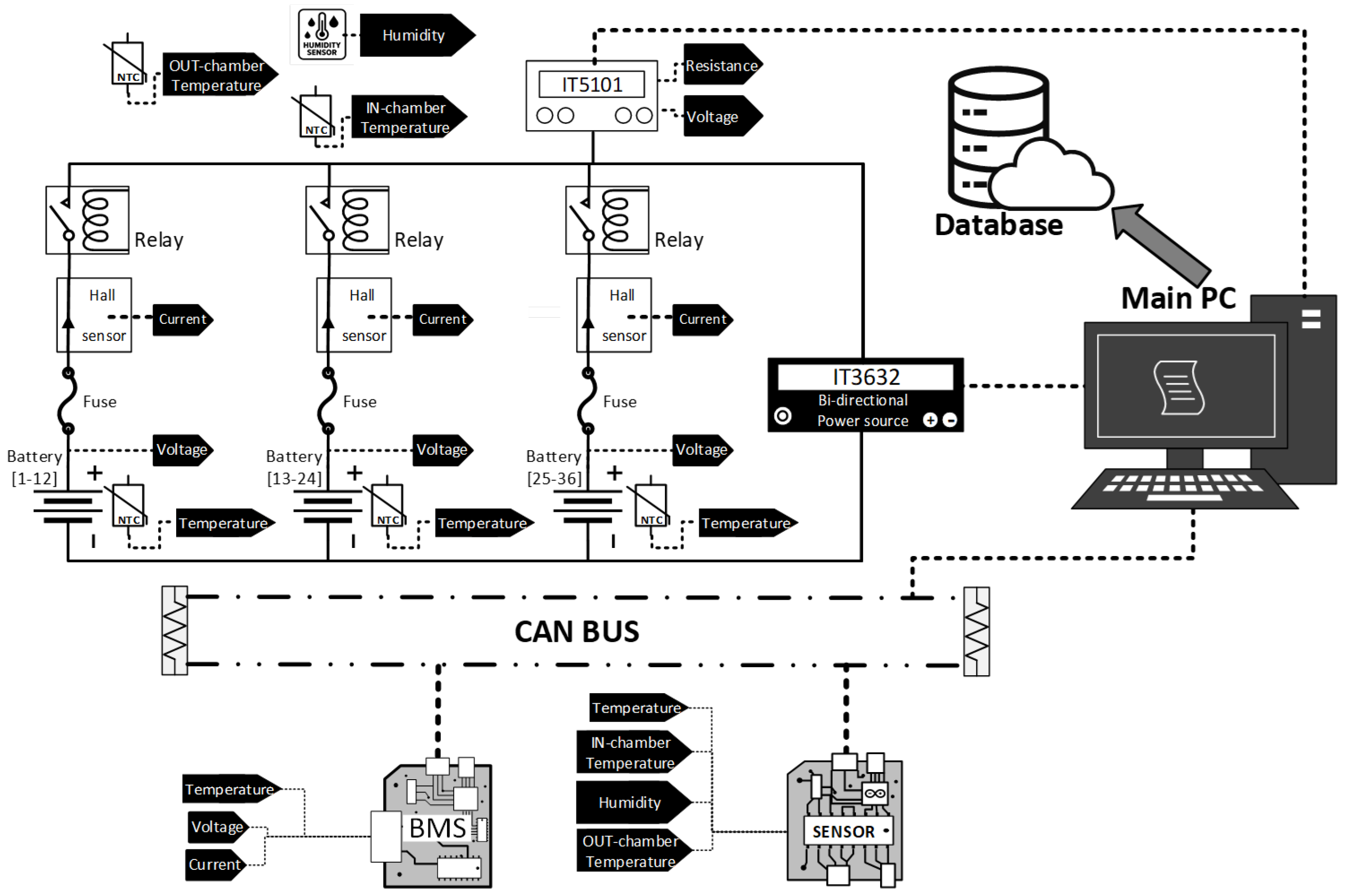
Figure 7.
Example of a driving cycle and a charge cycle obtained from the dataset.
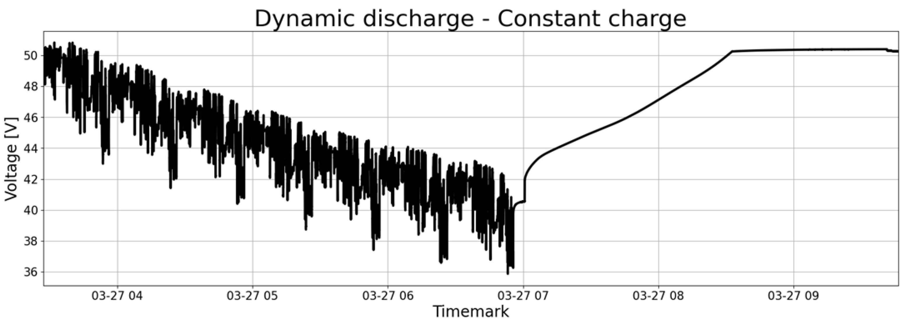
Figure 8.
Summary of the studies performed in this section.
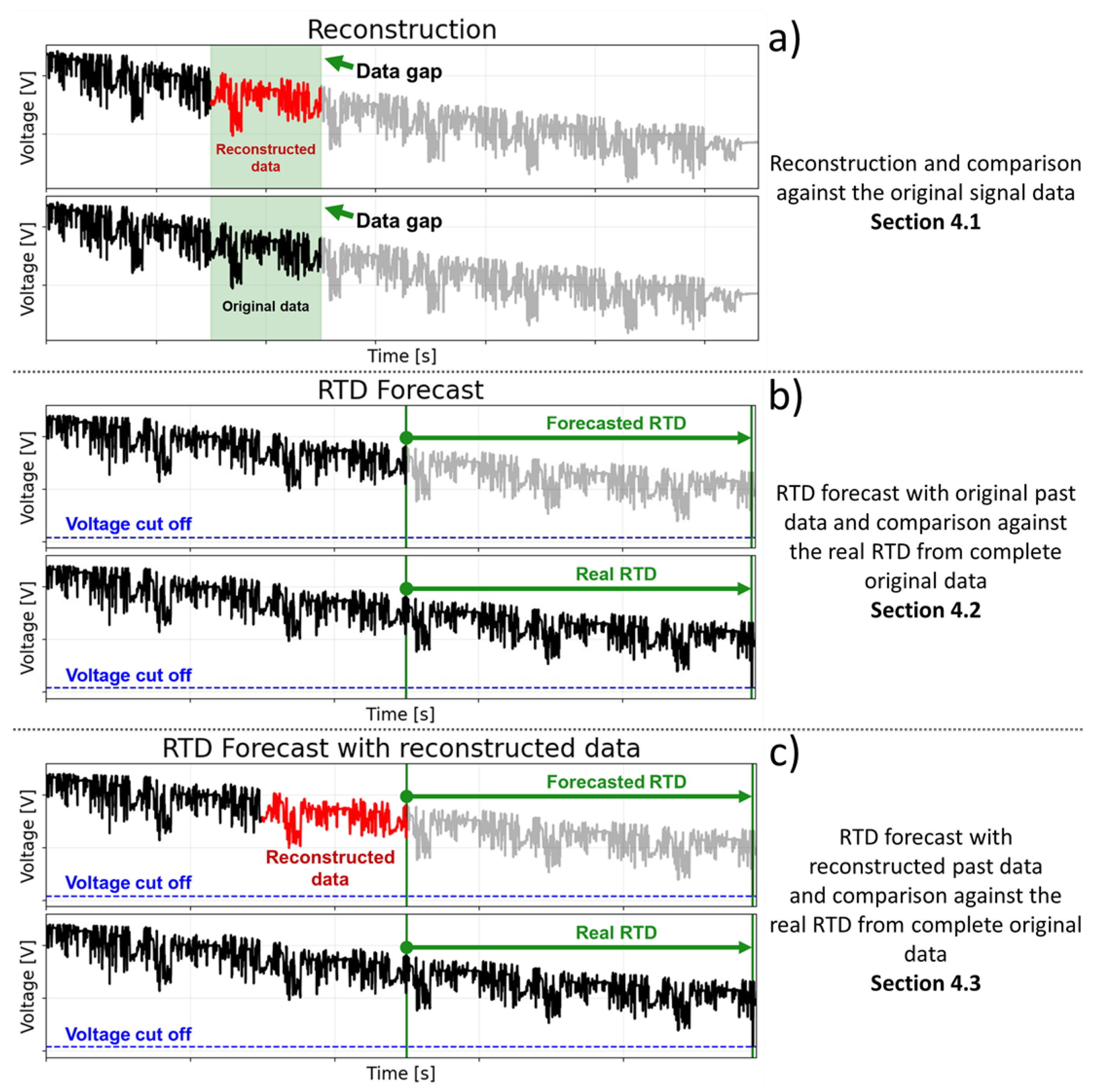
Figure 9.
ZOH, ARIMA, UKF and GRU reconstruction results for cycle 315 and cell S1P1 with a simulated artificial gap of 500 s.
Figure 9.
ZOH, ARIMA, UKF and GRU reconstruction results for cycle 315 and cell S1P1 with a simulated artificial gap of 500 s.
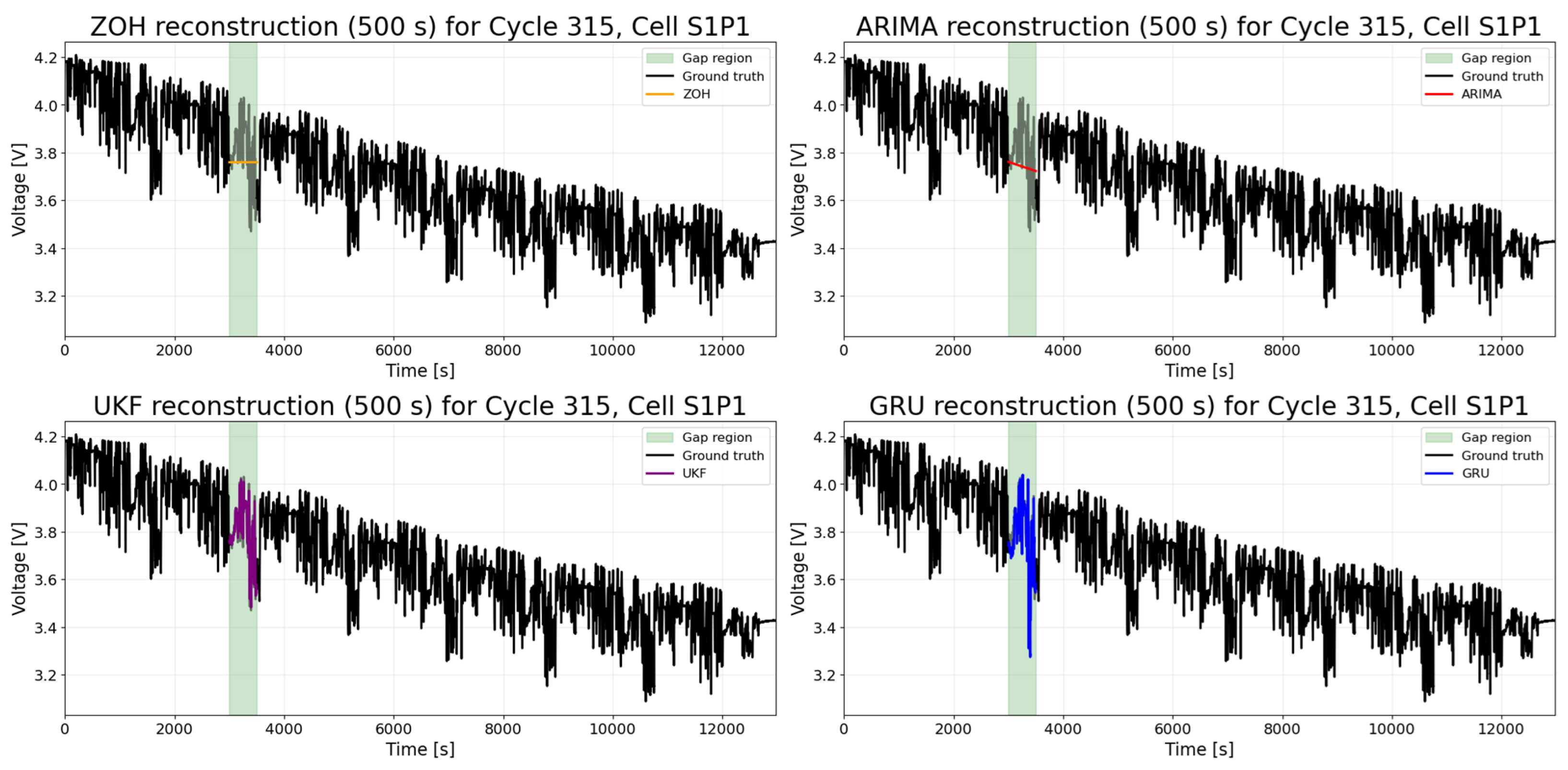
Figure 10.
Example of RTD forecast evaluation. At the top is the driving cycle discharge phase, with the voltage cutoff marked. Below is the RTD forecast error in seconds of
Figure 10.
Example of RTD forecast evaluation. At the top is the driving cycle discharge phase, with the voltage cutoff marked. Below is the RTD forecast error in seconds of
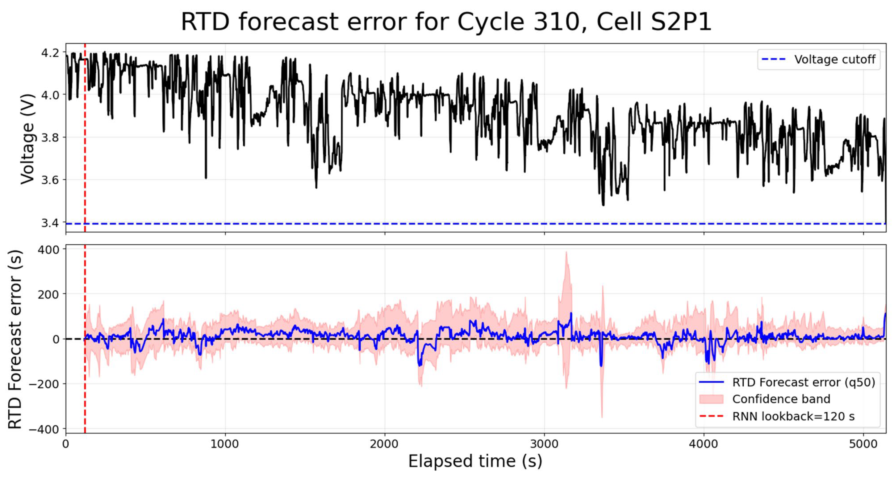
Figure 11.
Performance indicators of the RTD forecast based on the original signal of past data when compared with the RTD of the complete original signal. Boxplot results for the LSTM and GRU models. On the left, MAE in seconds for the forecasted
Figure 11.
Performance indicators of the RTD forecast based on the original signal of past data when compared with the RTD of the complete original signal. Boxplot results for the LSTM and GRU models. On the left, MAE in seconds for the forecasted
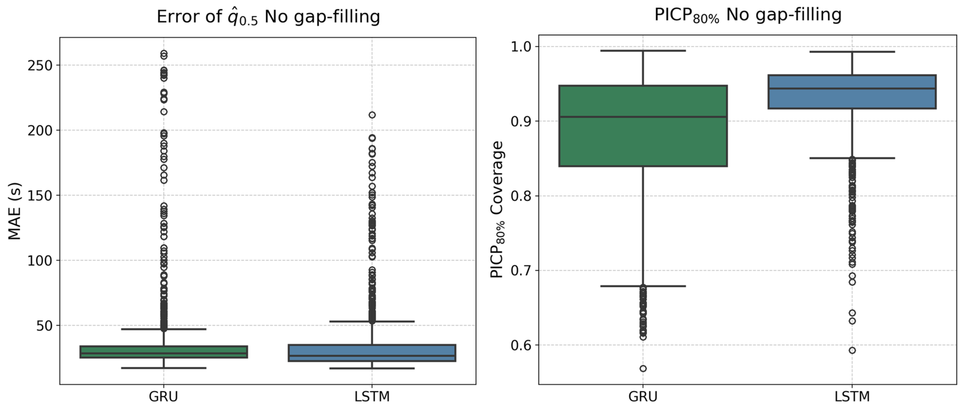
Figure 12.
Performance indicators of the RTD forecast based on the reconstructed signal of past data when compared with the RTD of the complete original signal. Boxplot results for the GRU models used for RTD forecasting based on the different reconstruction methods (UKF, GRU, ZOH and ARIMA)). On the left, MAE in seconds for the forecasted
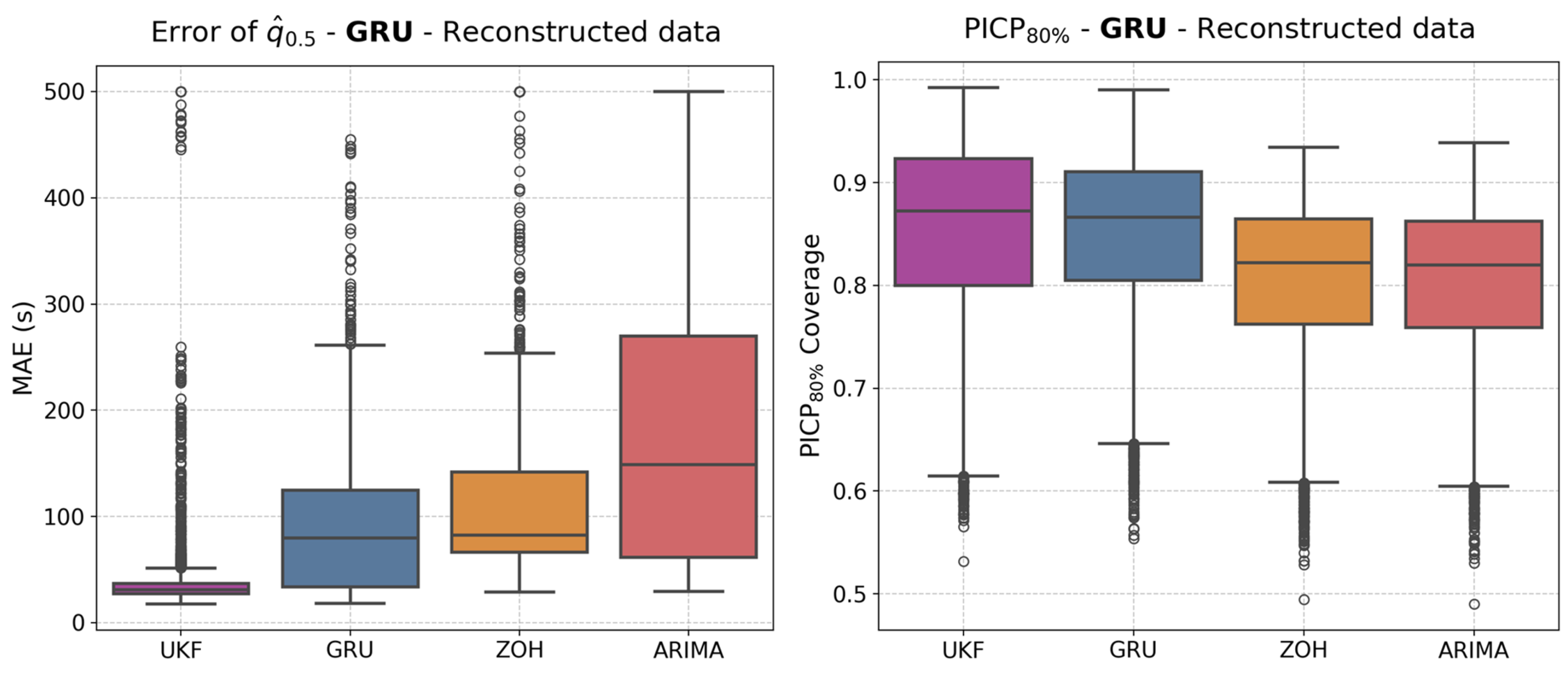
Figure 13.
Performance indicators of the RTD forecast based on the reconstructed signal of past data when compared with the RTD of the complete original signal. Boxplot results for the LSTM models used for RTD forecasting based on the different reconstruction methods (UKF, GRU, ZOH and ARIMA)). On the left, MAE in seconds for the forecasted


Table 1.
Performance metrics of the different evaluated reconstruction methods over 500-second data gaps that were simulated at the beginning, middle and end intervals of 40 discharge cycles for 36 cells, accounting for 4320 cases per method.
Table 1.
Performance metrics of the different evaluated reconstruction methods over 500-second data gaps that were simulated at the beginning, middle and end intervals of 40 discharge cycles for 36 cells, accounting for 4320 cases per method.
| Model | Average R2 | Average RMSE | Average MAE |
| ARIMA | -1.7104 | 0.0797 | 0.0813 |
| GRU (RNN) | 0.7936 | 0.0385 | 0.0287 |
| UKF | 0.9134 | 0.0266 | 0.0127 |
| ZOH | -1.1822 | 0.0764 | 0.0783 |
Table 2.
Values of the performance indicators of the RTD forecast based on the original signal of past data when compared with the RTD of the complete original signal.
Table 2.
Values of the performance indicators of the RTD forecast based on the original signal of past data when compared with the RTD of the complete original signal.
| Model |
mean values (s) |
median values (s) |
PICP80% mean values (%) |
PICPwidth mean values (s) |
|---|---|---|---|---|
| GRU | 36.2 s | 28.6 s | 88.2% | 159.06 s |
| LSTM | 34.5 s | 26.7 s | 93.1% | 126.56 s |
Table 3.
Values of the performance indicators of the RTD forecast based on the reconstructed signal of past data when compared with the RTD of the complete original signal.
Table 3.
Values of the performance indicators of the RTD forecast based on the reconstructed signal of past data when compared with the RTD of the complete original signal.
| Model | Reconstruction method |
mean values (s) |
median values (s) |
PICP80% mean values (%) |
PICPwidth mean values (s) |
|---|---|---|---|---|---|
| GRU | UKF | 39.2 s | 30.9 s | 85.2% | 157.1 s |
| GRU | 88.5 s | 79.9 s | 84.8% | 159.6 s | |
| ZOH | 113.7 s | 82.5 s | 80.3% | 161.6 s | |
| ARIMA | 167.1 s | 148.8 s | 80.1% | 164.1 s | |
| LSTM | UKF | 37.8 s | 30.4 s | 90.4% | 125.9 s |
| GRU | 88.3 s | 90.1 s | 90.1% | 129.0 s | |
| ZOH | 105.6 s | 78.0 s | 84.3% | 122.0 s | |
| ARIMA | 153.5 s | 144.7 s | 84.4% | 121.4 s |
Disclaimer/Publisher’s Note: The statements, opinions and data contained in all publications are solely those of the individual author(s) and contributor(s) and not of MDPI and/or the editor(s). MDPI and/or the editor(s) disclaim responsibility for any injury to people or property resulting from any ideas, methods, instructions or products referred to in the content. |
© 2025 by the authors. Licensee MDPI, Basel, Switzerland. This article is an open access article distributed under the terms and conditions of the Creative Commons Attribution (CC BY) license (http://creativecommons.org/licenses/by/4.0/).
Copyright: This open access article is published under a Creative Commons CC BY 4.0 license, which permit the free download, distribution, and reuse, provided that the author and preprint are cited in any reuse.


