
Submitted:
05 February 2026
Posted:
24 February 2026
You are already at the latest version
Abstract
To mitigate environmental impact, specifically the CO2 emissions associated with conventional thermal and nuclear facilities, renewable energy sources are increasingly being adopted as primary alternatives. However, integrating these renewable sources into the utility grid poses a significant challenge, primarily due to the stochastic and nonlinear nature of weather. Consequently, it is imperative that power systems operate under an intelligent control model to ensure energy output meets strict power quality standards. In this context, accurate forecasting is a cornerstone of smart power management, particularly in off-grid architectures, where predicting Power Quality Parameters (PQPs) is fundamental for system optimisation and error correction. This study conducts a comprehensive comparative evaluation of nine different predictive architectures for estimating PQPs. The algorithms analyzed include LSTM, GRU, DNN, CNN1D-LSTM, BiLSTM, attention mechanisms, DT, SVM, and XGBoost. The central objective is to develop a reliable basis for the automated regulation and enhancement of electrical quality in isolated systems. The specific parameters investigated are power voltage (U), Voltage Total Harmonic Distortion THDu, Current Total Harmonic Distortion THDi, and short-term flicker severity (Pst). Data for this investigation were acquired from an experimental off-grid setup at VSB-Technical University of Ostrava (VSB-TUO), Czech Republic. To assess model performance, we utilised Root Mean Square Error (RMSE) as the primary accuracy metric, while simultaneously evaluating computational efficiency in terms of processing speed and memory consumption during testing.
Keywords:
renewable energy
; machine learning
; forecasting
; power quality
; off-grid system
; power quality parameters
; energy communities
1. Introduction
Community power energy is known worldwide and is sometimes called community energy systems or community-based energy. This term refers to energy production, distribution, and consumption approaches rooted in local communities’ cooperation and participation. Community energy uses sustainable and renewable resources not only to mitigate footprints but also to bolster operational efficiency and strengthen local energy autonomy and safety. Aspects such as local ownership, decision-making, and energy management are also crucial in community energy, which can benefit residents and businesses economically. The approach can also include energy efficiency and conservation programs in homes and businesses. Community energy has enormous potential to encompass photovoltaic (PV) and wind energy system technologies, hydrogen technologies, and electric vehicles with Vehicle-to-Grid (V2G) technology. Such decentralised energy frameworks have gained significant traction among regulators and industry experts, who view them as viable pathways for achieving a shift toward low-carbon infrastructure. Consequently, academic discourse has seen a surge in related terminology, giving rise to concepts variously labeled as energy communities, shared solar initiatives, or cooperative wind projects. However, a community of power energy projects faces several challenges, including technical, regulatory, financial, and social barriers. With growing interest in sustainable development and support from public policies and technological advances, community energy is becoming an increasingly important element of the energy mix in many countries, especially in the Czech Republic and other Central European countries [1,2].
One barrier to the widespread deployment of community energy is the difficulty of estimating the behaviour of the small microgrids that comprise it. The fundamental problem is that most microgrids rely on PV power as their primary source of electricity. This type of plant generates electricity based on local weather conditions. It is, therefore, a source of electricity that supplies electricity in a highly stochastic manner.
There are large volumes of data for forecasting processes, such as solar wind power forecasting, power quality parameter forecasting, and power load forecasting. e.g. in [3] proposed a model for forecasting voltage total harmonic distortion () using a dataset collected by smart meters. The study tested some forecasting models, and the outcome shows that the autoregressive and feed-forward neural networks have better results than others in forecasting.
In the South African context, [4] implemented a predictive framework to estimate fluctuations in caused by diverse renewable sources, such as wind, solar, hydro, and ocean energy. The methodology utilised moving window segmentation for feature extraction, followed by a Long Short-Term Memory (LSTM) deep learning network for the actual signal prediction. Their findings demonstrated that the LSTM architecture effectively forecasted with minimal error rates.
Alternatively, research by [5] developed a forecasting architecture utilising Artificial Neural Networks (ANN) to predict Current Total Harmonic Distortion () originating from PV systems. The authors evaluated six distinct model configurations, varying the count of hidden layers and input features. Optimal performance was achieved with a specific configuration that employed two hidden layers and three input parameters.
In [6], the authors investigated six hybrid model variations integrating Artificial Neural Networks (ANN) with Adaptive Neuro-Fuzzy Inference Systems (ANFIS) to predict both voltage and current harmonics. Model efficacy was validated through comparative analysis of their outputs. Furthermore, the study suggested replicating this methodology across diverse geographical locations to verify the reliability and robustness of the proposed designs.
Frequency, voltage, , and [7] assessed four distinct machine learning approaches—specifically, varying linear regression techniques, ensemble decision trees, and neural networks—for the purpose of predicting power quality. The target variables included power line frequency, voltage, and the total harmonic distortion for both voltage and current. When comparing computational efficiency and accuracy, the decision tree algorithms yielded precise predictions. Conversely, in terms of execution time, the neural network was the most computationally intensive, whereas the linear models were the fastest.
Comparative research in [8] evaluated four hybrid systems for power load forecasting, specifically pairing K-means and K-medoids clustering with either ANNs or Decision Trees. The methodology followed a three-stage process: clustering, distance measurement between samples and cluster centres, and the final forecasting phase. Performance evaluation relied on Mean Absolute Percentage Error (MAPE). The results indicated that the K-medoids algorithm integrated with ANN outperformed the others, achieving the lowest error rate of approximately 8%.
The authors of [9] proposed a novel demand power forecasting system rooted in Artificial Neural Networks (ANN), optimised via the Golden Ratio Optimisation Method (GROM). When benchmarked against conventional ANN architectures, the proposed system demonstrated a significant performance enhancement, improving prediction accuracy by 41%.
Research presented in [10] conducted a comparative evaluation between Deep Neural Networks (DNN) and Recurrent Neural Networks (RNN) targeting power demand prediction. The validity of their proposed framework was assessed over forecasting horizons spanning both days and weeks, utilising a historical dataset covering a four-year period.
A composite architecture utilising multi-layer Bidirectional Recurrent Neural Networks—specifically integrating Long Short-Term Memory (LSTM) and Gated Recurrent Units (GRU)—was investigated in [11] for the purpose of power load estimation. The system underwent testing across two distinct datasets, with empirical results demonstrating its superiority over existing methodologies.
Reference [12] conducted a comparative assessment of two distinct architectures—the Back-Propagation (BP) neural network and the Elman neural network—for the purpose of short-term power load estimation. The outcomes of this investigation indicated that the Elman network performed better than the standard BP model.
Focusing on the power grid in Great Britain, [13] utilised a Long Short-Term Memory (LSTM) framework to predict grid frequency fluctuations. By applying multiple performance metrics, the study validated the efficacy and reliability of the proposed approach.
In a Turkish case study [14], researchers implemented and contrasted two specific models, Long Short-Term Memory (LSTM) and Gated Recurrent Units (GRU), to forecast . The system inputs integrated active power, current harmonics, and calendar data. The findings revealed that the LSTM architecture provided higher accuracy, resulting in lower error rates than the GRU model.
Quantile Regression (QR) was deployed in [15] to predict short-term current harmonics. When tested on real-world data from a low-voltage power grid, the proposed method demonstrated a significant improvement in prediction accuracy, reducing errors by approximately 21%.
[16] introduced a hybrid methodology named "Mycielski-Markov" for solar generation forecasting. This architecture synthesises the Mycielski signal processing algorithm with probabilistic Markov chains. The evaluation concluded that the system performed reliably, achieving a Coefficient of Determination () of approximately 0.87.
The integration of Genetic Algorithms with Support Vector Machines (GASVM) to predict short-term PV power output was investigated in [17]. Performance was assessed via Root Mean Square Error (RMSE) and Mean Absolute Percentage Error (MAPE), with results showing that the optimized GASVM surpassed the predictive capabilities of the standard SVM.
In the context of wind power in China, [18] developed a composite model incorporating wavelet transforms, Deep Convolutional Neural Networks (CNNs), and ensemble methods. Verified against empirical wind farm data, the study demonstrated the model’s capacity to effectively capture and learn the inherent uncertainties within wind energy generation.
Finally, [19] evaluated a deep learning approach utilising Long Short-Term Memory (LSTM) algorithms for solar power forecasting. This method was benchmarked against a Multi-Layer Perceptron (MLP) network using criteria such as Mean Absolute Error (MAE), MAPE, RMSE, and R-Squared (). The conclusion highlighted the LSTM model’s superior predictive performance compared to the MLP in the context of solar energy.
Research conducted by [20] utilised a Nonlinear Autoregressive Neural Network (NAR) to predict reactive power fluctuations. The architecture underwent rigorous testing involving varying input vector dimensions and diverse neuron configurations within the hidden layer. Ultimately, the investigation substantiated the efficacy of this proposed model for accurately forecasting reactive power in electrical grid systems.
A hybrid architecture integrating Variational Mode Decomposition (VMD), Gated Recurrent Units (GRU), and Time Convolutional Networks (TCN) was investigated in [21] for short-term power load prediction. By benchmarking against established methods such as LSTM, Prophet, and XGBoost, the authors demonstrated the model’s reliability. Specifically, the proposed hybrid approach significantly enhanced precision, lowering forecasting errors to 36.20% and 10.8% across two distinct datasets.
The integration of K-means clustering with Support Vector Machines (SVM) for short-term load estimation was proposed in [22]. In this workflow, K-means was used to partition the dataset into two distinct clusters, which were then processed by the SVM for final prediction. Empirical data indicate that this dual-stage system offers superior performance in both prediction accuracy and computational efficiency compared to conventional methodologies.
To refine the precision of short-term load forecasts, [23] introduced a hybrid framework merging Convolutional Neural Networks (CNN), LSTM, and attention mechanisms. When applied to demand power prediction across two thermal power plants, this attention-enhanced model (CNN-LSTM-A) demonstrated a marked advantage over standard LSTM architectures. The study reported accuracy improvements of 7.3% and 5.7%, respectively.
In an Australian case study, [24] developed a deep learning ensemble designed for wind power forecasting. The architecture comprised convolutional layers, GRU layers, and a fully connected neural network. The system’s efficacy was rigorously tested on two datasets against alternative models, including SVM, LSTM, ARIMA, and standalone GRU. Simulation results showed that this hybrid design yielded the most accurate predictions, reducing Mean Absolute Error (MAE) by up to 1.59% compared to the baselines.
In [25], a Multilayer Perceptron (MLP) Artificial Neural Network was employed to predict Total Harmonic Distortion () within power grids. The research involved an extensive optimisation process, varying the input variables, hidden layer counts, and neuron density. The optimal configuration—utilising two hidden layers with current, apparent power, reactive power, and active power as inputs—attained a peak correlation coefficient of 95.5%.
A study in [26] proposed a hybrid system for forecasting short-term power load. The model combined adaptive mode decomposition with improved support vector machines and a genetic algorithm to optimise the SVM weights. The system achieved an MAPE error of 1.78%, slightly better than others.
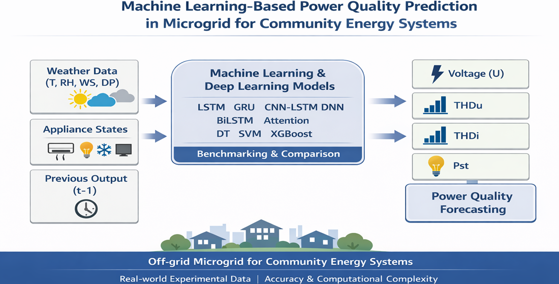
The core objective of this work is to accurately model the behaviour of energy parameters within microgrids, thereby enabling proactive responses to potential system disturbances. Consequently, this article focuses on forecasting selected power quality parameters by systematically benchmarking nine predictive models. These models span classical machine learning approaches (DT, SVM, XGBoost) and advanced deep learning architectures (LSTM, GRU, DNN, CNN1D-LSTM, BiLSTM, and attention-based networks). Particular emphasis is placed on DT, SVM, and LSTM as representative baseline models for analysing accuracy–complexity trade-offs. This research represents the initial phase of a broader investigation into predicting power quality for community energy systems. The present study employs a smaller-scale experimental architecture, the Researcher’s Microgrid Platform (RMP) at VSB-TUO, to validate and compare forecasting methodologies under controlled conditions. This approach allows for rigorous algorithm assessment and model refinement before scaling to more complex infrastructures. The subsequent phase of this research will extend the validated methodologies to the advanced facilities of the Centre for Energy and Environmental Technologies - Explorer (CEETe) at VSB-TUO.
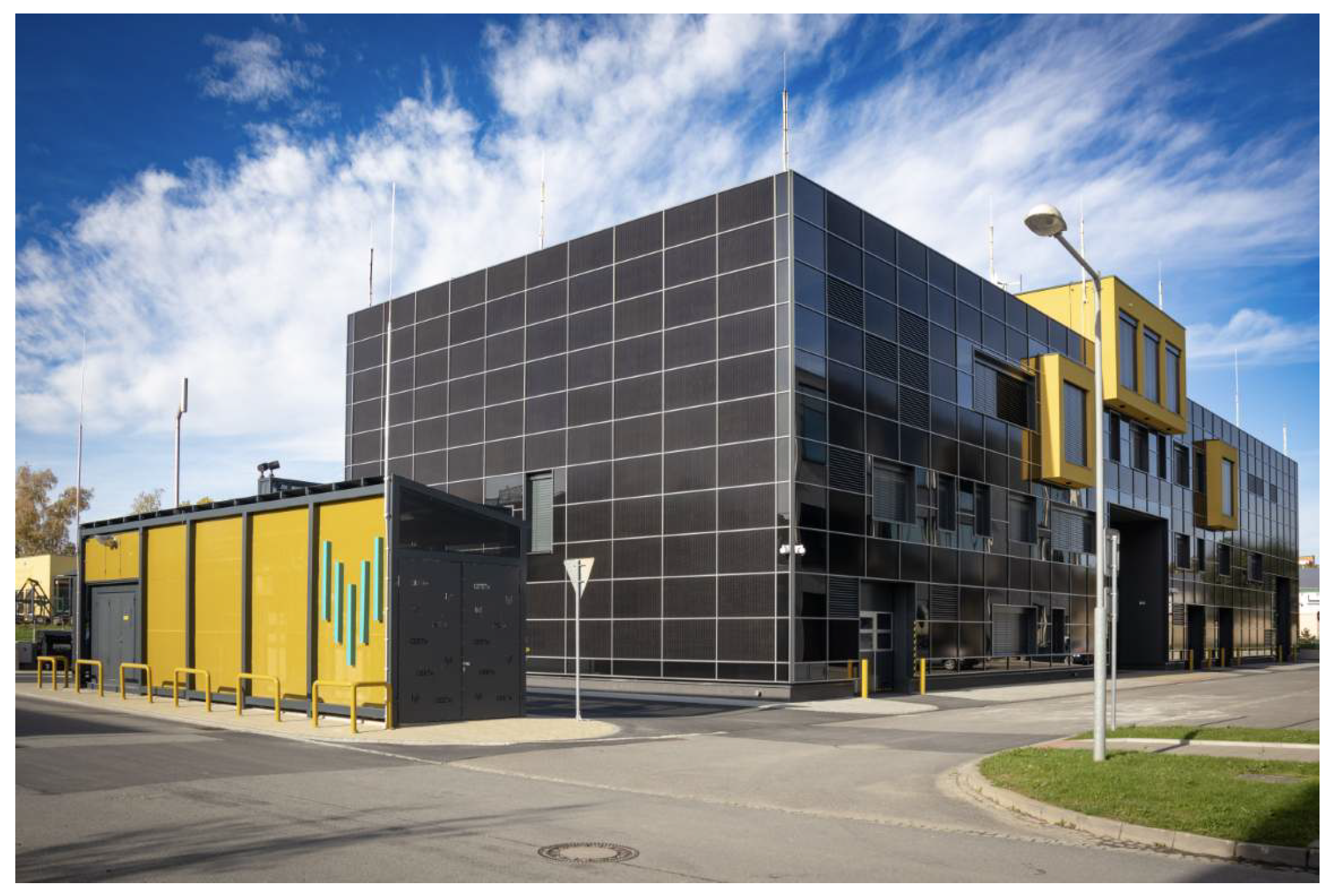
CEETe provides comprehensive research infrastructure encompassing four key areas: energy accumulation, transformation and control; materials for energy and environmental technologies; utilisation of secondary resources and alternative energy sources; and environmental aspects and technologies. This progression from pilot-scale testing to full-scale implementation within CEETe’s integrated research environment will enable comprehensive validation of forecasting models across diverse microgrid configurations and community energy architectures, ultimately contributing to the development of robust power quality management systems for decentralised energy communities.[27]
Figure 1.
CEETe – Community Energy Systems Research [27]
Figure 1.
CEETe – Community Energy Systems Research [27]
The main novel contributions of this study are summarized as follows:
- A unified benchmarking framework for the simultaneous forecasting of multiple power quality parameters, namely power voltage (U), voltage total harmonic distortion (), current total harmonic distortion (), and short-term flicker severity (). Unlike most existing studies that focus on a single power quality indicator, this work evaluates model performance across several interrelated parameters within the same microgrid environment.
- A joint evaluation of forecasting accuracy and computational complexity, where prediction performance is assessed not only in terms of Root Mean Square Error (RMSE), but also with respect to execution time and memory consumption during the testing phase. This dual-perspective analysis provides practical insights into the suitability of machine learning and deep learning models for real-time and resource-constrained microgrid control applications.
- Experimental validation using real-world measurements obtained from a residential-scale off-grid microgrid platform. The dataset reflects actual operating conditions, including renewable generation variability, household appliance usage, and measured power-quality disturbances, thereby enhancing the practical relevance and transferability of the results.
The article is divided into seven sections. Section 1 introduces the main topic, the author’s motives, goals, and previous related studies. Section 2 describes the description of the experimental platform. Section 3 describes the mathematical description of the models used in this article. Section 4 explains the designed method. Section 5 presents the results of the study. Section 6 analyses the results of the experiment, and Section 7 represents the conclusion of the article.
2. Platform Description
The research utilised the Researcher’s Microgrid Platform (RMP), which simulates a standard residential household in the Czech Republic. The RMP is located on the VSB-TUO Campus. It operates in off-grid mode and connects to the distribution grid when energy is not available. The platform is being developed with links to smart grids and the energy sector. In this experiment, only the RMP component is included, but Figure 2 illustrates the overall concept of this technology.
The location of renewable sources in the physical model of the microgrid is shown in Figure 3. The main energy source for the RMP is the electricity generated by the two-watt PV string and, if necessary, the distribution network. The RMP is an off-grid system based on a hybrid AC/DC BUS architecture. Located around a hybrid inverter, the infrastructure supports a rated power of 6.8 kW. The AC part is powered by a 230 V BUS, and the DC part is powered by a 48 V BUS. The main parameters of this hybrid inverter can be seen in Table 1, and the main parameters of the PV MPPT inverter can be seen in Table 2. Figure 4 Hybrid inverter Conext XW+ 8548 and PV inverters Xantrex XW 80 600 [30]
The RMP stationary batteries are shown in Figure 5. The battery type is Hawker 12XFC115, with a nominal voltage of 12 V and a nominal capacity of 115 Ah. The RMP storage batteries are connected in a serial-parallel configuration into four groups, each containing four batteries. Power Quality (PQ) measurements using the KMB SMC 144 PQ analyser on the AC BUS. The data is stored on the server.
Table 4 shows a list of appliances used in the experiment. The main parameters of the RMP battery can be seen in Table 3.

| Description | Value |
|---|---|
| Nominal Voltage | 12 V |
| Nominal Capacity C5 | 115 Ah |
| Nominal Capacity C20 | 128 Ah |
| Cycle life (DOD 60 %) | 1200 Cycles |
| Weight | 43.0 kg |
Table 4.
Table of appliances/home consumption [7]
Table 4.
Table of appliances/home consumption [7]
| Appliance/Consumption | (kW) | (-) | (%) | ||||
|---|---|---|---|---|---|---|---|
| Avg | Min | Max | Avg | Character | |||
| No appliance | - | - | - | - | - | 2.1 | 42.1 |
| Kettle | 619.1 | 617 | 628.3 | 1 | R | 4.2 | 6.2 |
| Fridge | 207.6 | 195.5 | 219.5 | 0.7 | L | 2.8 | 11.7 |
| Air Conditioning | 880 | 852.5 | 910 | 0.9 | L | 2.2 | 10.1 |
| Microwave | 203 | 76.8 | 1348 | 0.8 | L | 5.1 | 56.8 |
| LCD TV | 44 | 42.8 | 50.5 | 0.6 | C | 3.0 | 20.9 |
| Lights | 156 | 152.5 | 165.1 | 0.8 | C | 2.8 | 77.6 |
3. Formal Methods
3.1. Support Vector Machine (SVM)
Support Vector Machines represent a category of supervised learning algorithms utilised for both categorical labelling and continuous value estimation. In a regression context, the algorithm identifies an optimal hyperplane that encompasses the maximum number of data points within a defined boundary, effectively capturing the underlying trends of the time-series data while bounding the prediction error. [33,34,35]. In classification, the objective is to discover a hyperplane that effectively divides data points into distinct categories [34]. In regression, the goal is to identify a hyperplane that accurately captures the data with a wide margin surrounding it [35].
In the Support Vector Machine, the two most fundamental concepts are Margins and Support Vectors [36]: The ’margin’ is the distance between the hyperplane and the closest data points on either side (these are the support vectors). SVMs aim to maximise this margin, leading to better generalisation.
Regarding SVM for regression (Support Vector Regression, SVR), it can be used as a time-series prediction model, as it finds the hyperplane that best fits the data points while minimising error. Thus, it can handle non-linear relationships in the data and is therefore effective at capturing complex patterns in time-series data.
In this study, SVR will be used to predict continuous numeric values like power voltage, , , and .
- The goal of SVR is to create a function that can forecast a continuous target output, as well as maximise the margin between the forecasted and measured samples.
- SVR determines a margin around the forecasting line, while the objective is to create a line inside this margin, as well as minimising the error between actual and predicted values.
- Data points that are very near the regression line are called support vectors, and these vectors have an important role in creating the regression approach.
Suppose the dataset for creating the model is as follows: input features () and the target output are ()
The main goal of SVR is to build a model (), that will forecast the target output (y).
3.2. Long Short-Term Memory (LSTM) Networks
Recurrent Neural Networks (RNNs) are a class of deep learning models widely used for tasks involving sequential data and time-series analysis. Their application spectrum is broad, encompassing natural language processing and speech recognition [37,38], as well as visual content interpretation such as image captioning [39,40,41,42] and video analytics [43,44]. Distinct from standard networks, RNNs are engineered to process sequences by establishing recurrent connections that effectively create an internal memory of antecedent inputs. This mnemonic capacity enables the system to accommodate input sequences of variable durations and to extract temporal dependencies embedded within the data. Consequently, in the realm of time-series forecasting, RNNs are capable of synthesising historical data points to project future trends
To address the "vanishing gradient" issue found in standard , the Long Short-Term Memory (LSTM) and Gate recurrent unit (GRU) cells utilise a gated architecture. These components—the input, forget, and output gates—regulate the flow of information, allowing the model to retain dependencies across extensive temporal sequences [45,46].
Between these two cells, LSTM is the most popular integrated cell in RNNs due to its ability to learn longer sequences with more complex patterns, whereas GRU is only suitable for short sequences with simple patterns. Since our research’s power quality parameters are signals with very long sequences and complex patterns, LSTM is the most suitable choice for our Deep learning approach experiment.
Structurally, an LSTM unit is defined by four core elements: a central Cell state and three regulatory mechanisms, known as gates (the Forget, Input, and Output gates) [47]. These gates function as sophisticated filters that modulate data flow. In theoretical terms, their specific roles are: the Input gate regulates the admission of new data into the memory cell; the Forget gate identifies and purges irrelevant information from the cell; and the Output gate dictates the final signal to be emitted by the LSTM unit.
To formalise the mathematical framework, we let X represent the sequential input data, while h and c denote the hidden state and cell state, respectively. The temporal notation uses to indicate the current time step and to represent the immediate predecessor. The learnable parameters are categorised into three sets corresponding to the gates: the forget gate parameters (), the input gate parameters (), and the output gate parameters (). These weight matrices and bias vectors are essential for preserving and transforming information derived from the previous hidden state [48]. Furthermore, and correspond to the sigmoid and hyperbolic tangent activation functions, respectively. The interaction between these three gates and their internal mechanisms is visually depicted in Fig. 3 [47,48,49] below
Figure 7.
A typical Long Short Term Memory (LSTM) cell.
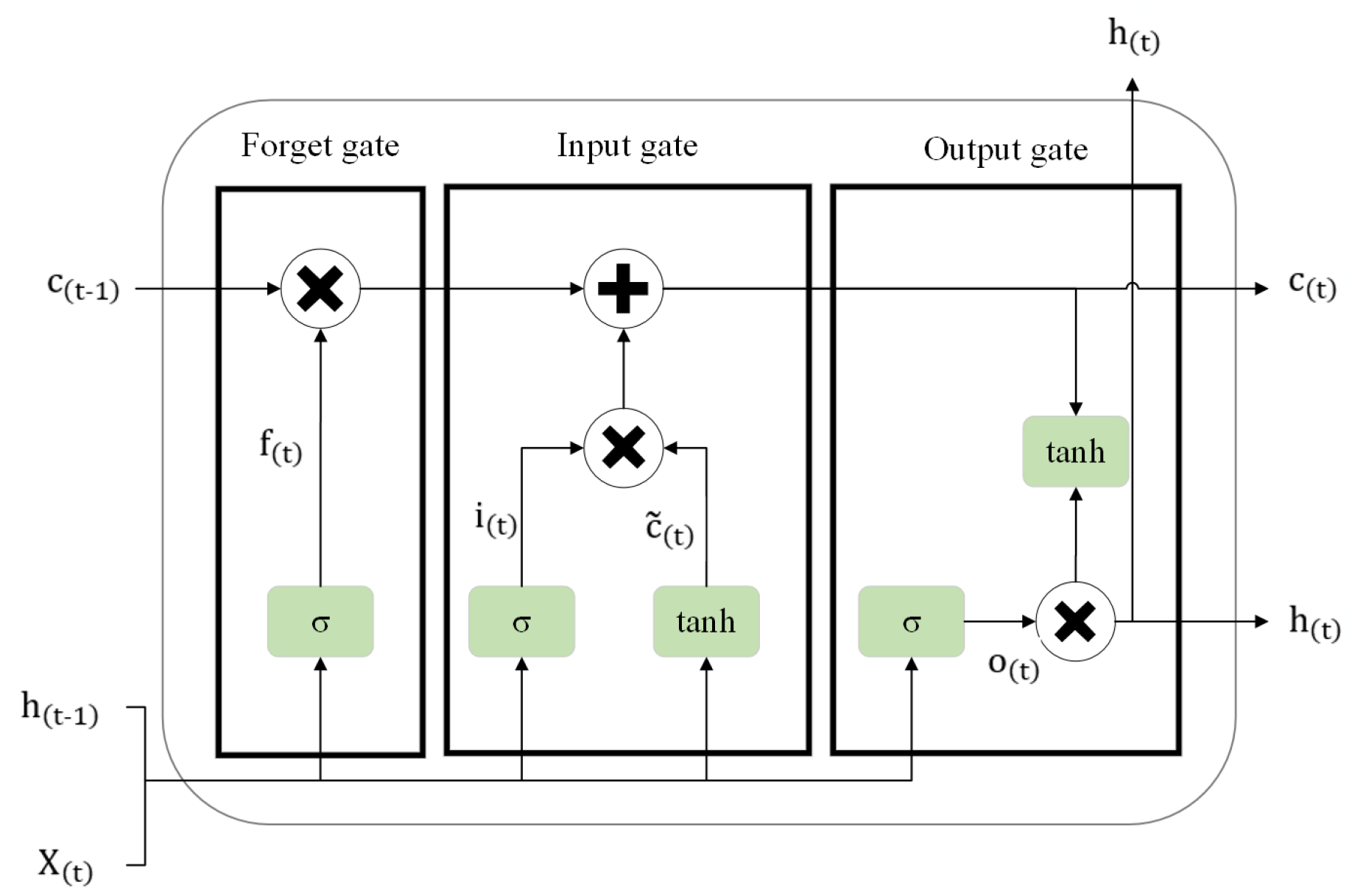
The Forget Gate: Represented by , this mechanism filters the cell state to remove irrelevant data. It employs a sigmoid function to output a value between 0 and 1; effectively, a value of 0 implies complete erasure of the previous information, while 1 signifies complete retention.
The Input Gate: Denoted as , this component regulates the extent to which new information is incorporated into the memory cell.
The Output Gate: Symbolised by , this gate controls the flow of information from the current cell state to the subsequent hidden state, filtering the internal data to determine the final output.
We define as the output of the layer within the input gate; this represents a vector of new candidate values that could potentially be added to the cell state. Furthermore, we denote the operator as the Hadamard product (element-wise multiplication) and as the hyperbolic tangent activation function. Consequently, the final cell state and the hidden state are computed via the following expressions:
Figure 8 depicts the comprehensive architecture of the LSTM framework developed for this study.
Regarding the internal structure, the model incorporates a dual-layer LSTM configuration designed to identify temporal correlations within the training and testing sequences. Subsequently, two dense layers are employed to integrate these extracted features into a unified vector prior to the final output stage. The input tensor is defined with the dimensions (None, 1, 7); this indicates that the model processes sequences containing seven distinct input variables to generate a forecast for a single future time step.
To optimise the network parameters—specifically the weights and biases associated with the gates and cell states—the system utilises forward and backward propagation algorithms. In the context of RNNs, the optimisation technique is distinctively known as Backpropagation Through Time (BPTT). This method works by conceptually expanding the network’s structure across the temporal dimension to handle sequences, enabling weight updates at every time step. This contrasts with standard backpropagation typically found in spatial neural networks. BPTT is the critical mechanism that enables RNNs, and by extension LSTMs, to adjust parameters while preserving the sequential integrity of the input data. Further theoretical details regarding BPTT can be explored in [50]
3.3. The Gated Recurrent Unit (GRU)
An alternative architecture within the RNN family is the Gated Recurrent Unit (GRU). Designed as a streamlined evolution of the LSTM, the GRU effectively mitigates the vanishing gradient phenomenon common in traditional RNNs. Unlike the LSTM, the GRU operates without a distinct cell state and utilises a simplified gating structure. This architectural efficiency enables the model to capture long-term temporal dependencies with reduced computational overhead.
The operational logic of the GRU is primarily governed by two specific control mechanisms: the update gate and the reset gate. The functional steps are detailed in [51,52] as follows:
1) Update Gate (): This component regulates the retention of historical data, determining the extent to which information from previous time steps is preserved for the future.
2) Reset Gate (): Functioning as a filter, this gate identifies which aspects of the previous information are irrelevant and should be discarded.
3) Candidate Activation (): This represents the provisional hidden state, encompassing new features extracted from the input and the reset-filtered history.
4) Final Memory at Time t (): The resulting hidden state is computed as a linear interpolation between the previous state and the new candidate activation.
where: - : Represents the Update gate - : Represents the Reset gate - : Denotes the Candidate hidden state - : The current hidden state output - : The input vector at time step t - : The hidden state from the preceding time step - : The learned weight matrices associated with each gate - : The Sigmoid activation function - tanh: The Hyperbolic tangent activation function - ⊙: The operator for element-wise multiplication.
3.4. The Structure of 1-Dimensional Convolutional Long Short-Term Memory Conv1D-LSTM
This hybrid architecture synergises the 1-Dimensional Convolutional (Conv1D) layer with the LSTM network. Initially, the Conv1D module applies convolutional filters to the input sequence to isolate local patterns and features. The resulting output effectively serves as a high-level feature map. Following this extraction phase, the data is forwarded to the LSTM layer, which analyses the sequential feature maps to identify and learn long-term temporal dependencies. The computational process for this composite 1-Dimensional Convolutional Long Short-Term Memory (Conv1D-LSTM) model is bifurcated into two phases, calculated as follows [53,54,55]:
1) Compute 1D Convolution Operation:
where: is the output of the convolution at time t, is the input sequence at time t, K is the size of the convolution kernel, is the weights of the convolution kernel, and b is the bias term.
2) Combine with the LSTM calculation: To combine Conv1D with LSTM, the Conv1D layer is applied to the input of the input sequence before passing the resulting feature maps to an LSTM layer. The equations then become:
Then, all the in equations from (2) to (7) will be replaced with to create the Conv1DLSTM as below. Notice that * is the convolution operation between two parameters.
Input Gate:
Forget Gate:
Cell State Update:
Output Gate:
Hidden State Update:
The CNN1D extracts features from the input sequence, which the LSTM then processes to capture temporal dependencies in both two dimensions.
3.5. The Bidirectional Long Short-Term Memory
In a Bidirectional Long Short-Term Memory (BiLSTM), two LSTM layers are created: one processes the input sequence from the start to the end (forward LSTM), and the other processes it from the end to the start (backward LSTM). The outputs from both layers are then concatenated or summed to form the final output. The computation of BiLSTM is described as [56,57,58]:
Let be the hidden state from the forward LSTM and be the hidden state from the backward LSTM. The final output at time t is given by:
Where ⊕ represents the concatenation operation.
Putting it all together, the equations for a BiLSTM can be summarised as:
Forward LSTM:
Backward LSTM:
Final Output:
3.6. The RNNs with Attention Mechanism
In RNNs that use GRUs or LSTMs, attention mechanisms help these models focus on specific parts of the input sequence when generating outputs. The key functions of attention in RNNs are Dynamic Focus: Instead of processing the entire input sequence equally, attention allows the model to weigh the importance of different inputs at each time step, enabling it to focus on relevant information; Handling Long Sequences: Attention helps RNNs manage longer sequences more effectively by allowing them to bypass limitations related to memory and vanishing gradients, which can occur in standard RNNs; and Improved Performance: By selectively attending to relevant parts of the input, attention mechanisms can lead to better performance in tasks like translation, summarization, and image captioning. These functions help the RNNs to model complex dependencies in sequential data [59,60].
Given an input sequence of vectors , the RNN processes these vectors to produce hidden states . The RNN with attention layer’s work can be shortly described as follows [59,60,61]:
Calculating Attention Scores: For each hidden state (where t is the current time step), we calculate attention scores for each input :
The scoring function can be a simple dot productnormalised, a feedforward neural network, or any other function that quantifies the relevance of to .
Softmax Normalisation: The attention scores are then normalized using the softmax function to obtain the attention weights :
Context Vector: The context vector for the current time step t is computed as a weighted sum of the hidden states:
Output Generation: Finally, the context vector is used along with the hidden state to generate the output :
3.7. The Extreme Gradient Boosting XGBoost
Extreme Gradient Boosting (XGBoost) is rooted in the ensemble boosting methodology, which constructs a robust predictive model by aggregating multiple ’weak’ learners, predominantly decision trees. The fundamental concept involves an iterative process where new models are introduced to rectify residual errors left by preceding iterations. While the computational mechanics of XGBoost are intricate, the core algorithm can be summarized as follows [62,63,64]:
1) Objective Function: The primary optimization target in XGBoost is formulated as:
In this context, L represents the cumulative loss, where n denotes the total sample count. The term l refers to the specific loss metric (such as Mean Squared Error), while and represent the predicted and actual values, respectively. Furthermore, K signifies the total count of trees, and denotes the regularization penalty applied to the k-th tree .
2) Regularization: To govern model complexity and mitigate overfitting, a regularization term is employed, defined by:
Here, T corresponds to the leaf count within a tree, and represents the leaf weights. The parameter acts as the threshold for minimum loss reduction necessary to authorize a new split, while serves as the L2 regularization coefficient.
3) Gradient and Hessian: To optimize the learning trajectory, XGBoost leverages the first-order (gradient) and second-order (Hessian) derivatives of the loss function. The iterative update rule for predictions is expressed as:
In this equation, represents the learning rate (shrinkage), and denotes the newly added tree structure at iteration t.
4) Tree Construction: The structural expansion of each tree is driven by maximizing the gain score, calculated via:
Within this formula, and correspond to the first and second derivatives of the loss function for instance j. Additionally, L and R identify the instance sets assigned to the left and right child nodes following a split.
3.8. Regression Decision Tree
A decision tree (DT) is one of the machine learning tools that has been applied successfully for classification and regression applications [65,66]. The three components of a decision tree are: Internal Nodes: Represent tests or questions on features (attributes) of your data. Branches: Represent the possible outcomes of each test. Leaf Nodes: Represent the final classification or prediction (i.e., the answers).
A regression decision tree creates a regression model in a tree mode. The process divides a dataset into small subsets with an associated decision and these subsets will split further into other small subsets till to the final step, results will be a tree structure consists decision nodes and leaf nodes. A decision node will split the sample into two or more branches, and a Leaf node has one numerical decision.
Learning Process: Decision trees are built by recursively splitting the data based on features that best separate the different classes or reduce prediction error [67]. In classification, the Gini Impurity, a measure of the homogeneity of the nodes, will be used to find the features that separate the data best [68]. In regression, instead, Decision trees typically use metrics like mean squared error or variance reduction to make splitting decisions [69]. Regarding the regression task, to avoid the complicity and the unnecessary long explanation, the learning process can be briefly described as [67]:
- 1.
- Root Node: As before, the entire dataset starts at the root.
- 2.
-
Splitting Criteria: regression Decision trees generally use variance reduction. This algorithm looks to minimize the variance of the target variable within each node in order to choose the split that leads to the greatest reduction in the variance of the target variable within the subsets. By choosing splits that result in the largest reduction in variance, the algorithm aims to create homogeneous subsets that lead to more accurate predictions. The variance reduction can be illustrated as:Where:S is the subset of data. Nis the number of instances in the subset. is the target value of instance i. is the mean target value in the subset
- 3.
- Recursive Partitioning: After the initial split, each subset is further divided into smaller subsets using the same splitting criteria. This process continues recursively until a stopping criterion is met, such as reaching a maximum tree depth or minimum number of samples in a node. Steps 2 and 3 are repeated on each newly formed subset.
- 4.
- Prediction: Finally, to make predictions on new data points, the input features are passed down the tree, and the average target value of the corresponding leaf node is used as the predicted output. When a stopping criterion is met, leaf nodes are created. Instead of assigning a class, each leaf node predicts the average target value of the training data points within that node.
4. Proposed Model
The study compared the performance of nine forecasting models: LSTM, GRU, DNN, CNN1DLSTM, B1LSTM, Attention, DT, SVM, and XGBOOST to forecasting four types of PQPs, these parameters are power voltage (U), total harmonic distortion of voltage (), total harmonic distortion of current (), and short-term flicker severity(). All models were evaluated using identical input features and prediction horizons to ensure a fair comparison across different power quality parameters.
4.1. Dataset
The dataset consists of two parts: The power dataset and the weather dataset. The dataset was available for every one-minute time step and provided from the off-grid system at VSB-TUO, the power dataset included the current consumption of home appliances and the status of the battery, U, , , and while the weather dataset included weather conditions: air temperature, dew point, Humidity, air pressure, wind speed.
4.2. Experiment Setup
The experiments were carried out using the following input variables air temperature, Dew Point, Humidity, air pressure, wind speed, previous value of the output, and states (on = 1, off = 0) of the 4 types of home appliances (AC heating, Lights, Fridge, TV). The states of home appliances (0 or 1) were converted into an equivalent decimal number, e.g. the device states 0 0 0 0 converted into equivalent decimal no 0, and 1 1 1 1 converted into 15, and likewise for the rest of the cases [70]. This encoding was adopted to reduce input dimensionality; however, all models were evaluated consistently using the same representation to ensure a fair comparison. The previous value of the output is mean one step back of the output used with input variables, e.g. in the voltage forecasting model for forecasting voltage at the time step t () with mentioned weather conditions and statutes of home appliances at the same time step t will add the previous value of the voltage (), as can be seen in the scheme of the proposed model in Figure 9, and variables description in Table 5.
5. Numerical Results
In this study, the root mean square error (RMSE), have been used for evaluating the tested models and comparing their performance as in (33).
where m, and r are the measured and model result values respectively, n size of data sample.
The forecasting results can be seen in Table 6, Table 7, Table 8, and Table 9, which showed the RMSE and RMSE average achieved by tested models of days 21, 22, and 23 of January 2023, for forecasting U, , and respectively.
When the experiments ran, the computational complexity (Execution time and usage Memory) for testing one sample was calculated in the testing phase for forecasting each parameter, as can be seen in Table 10.
6. Discussion
6.1. Forecasting Error
Root-mean-square deviation (RMSE) was used to evaluate and compare forecasting models’ performance.
The performance of the forecasting designed models was analysed and compared as follows:
- Power Voltage: The forecasting error of power voltage ranges from 0.16 to 1.71. As shown in Figure 10, good predicting accuracy for power voltage was observed in the , , and models, followed by the and architectures.
- : The RMSE of was verified between 0.1999 and 0.6337. Figure 11 shows the RMSE error of , when comparing the results, the smallest forecasting error was obtained from DNN, B1LSTM, Attention, LSTM, GRU, and then CNN1DLSTM. While xGBOOST, DT, and SVM achieved the biggest errors.
- : The performance of GRU, LSTM, CNN1DLSTM, DNN, Attention, and B1LSTM for forecasting was approximately the same and achieved an error between 5.02 to 5.20. Then came SVM and XGBOOST, with the DT ranked last, showing errors of 5.91 to 9.87, as seen in Figure 12.
- : Figure 13 shows the performance of GRU, LSTM, Attention, B1LSTM, DNN, and CNN1DLSTM for estimating close to each other and accomplish an error less than 0.1. Then came the XGBOOST, SVM, and DT, which accomplished an error between 0.27 to 1.06.
In Figure 14, another method can be seen that uses a radar graph to represent the comparison of the performance models.
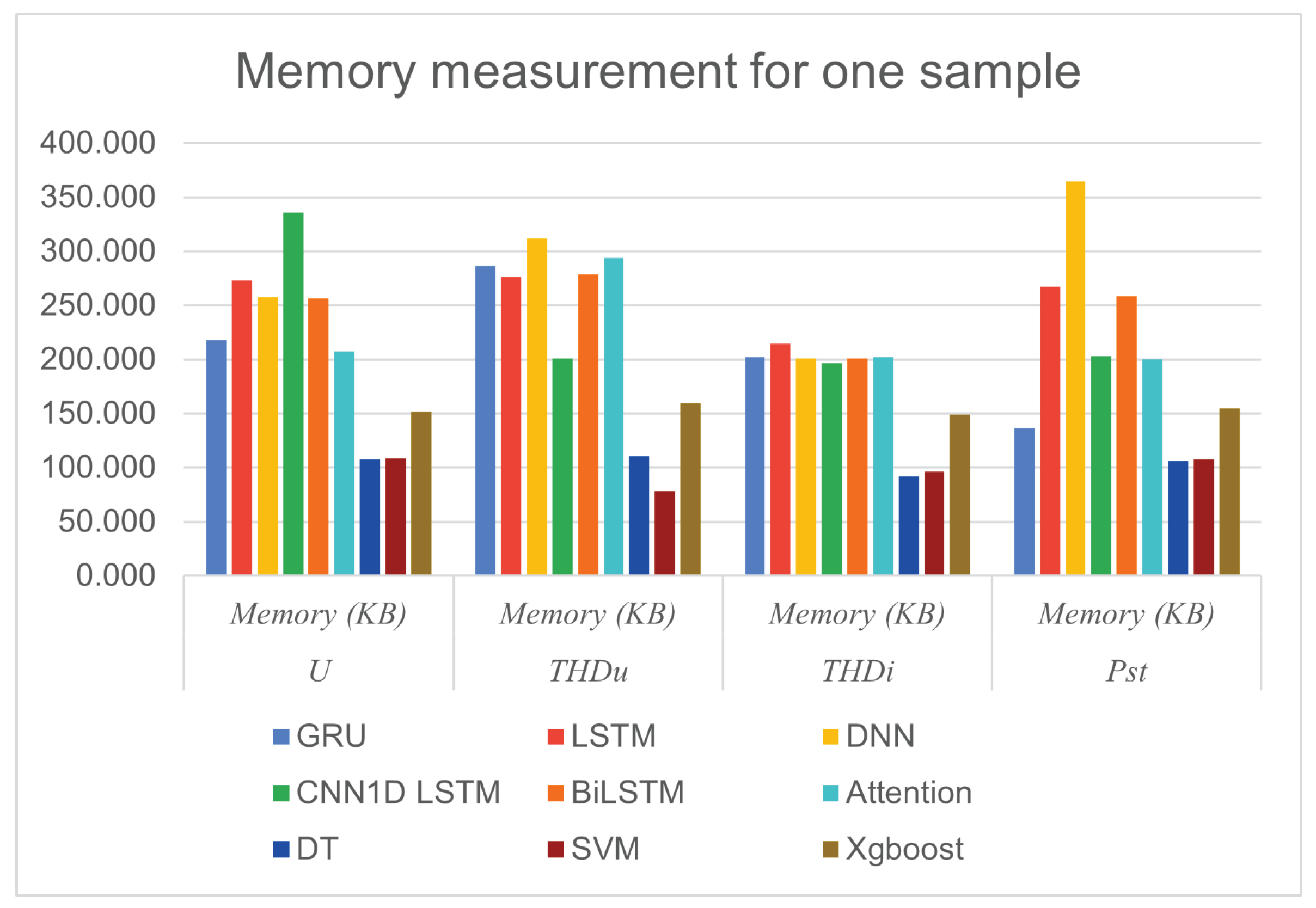
6.2. Computational Complexity
The computation time and memory usage in the testing phase were calculated to test one sample, as can be seen in Table 10, Figure 15, and Figure 16.
The Deep Learning neural network group of models uses more time and memory to execute 1 sample than the Machine Learning group of models.
Overall, DT and SVM emerge as the most efficient algorithms, excelling in both speed and memory usage. This makes them strong candidates for this task, especially in resource-constrained environments. DNN appears to be the least efficient in both time and memory, suggesting potential areas for optimisation or alternative model choices.
Deep Learning models, such as LSTM and DNN, while potentially slower and more memory-intensive, might offer higher accuracy or better performance in certain tasks, justifying the increased resource consumption.
These complexity measurements and previous accuracy measurement results clearly show the trade-offs between the two different types of models. While ML models can process faster with better memory efficiency, DL models provide more accurate predictions. The choice of which models to use depends on which strengths your system prefers most.
7. Conclusion
This article presents a systematic benchmark of machine learning and deep learning methods for multiple power quality parameters, complemented by a practical analysis of computational complexity on a real off-grid microgrid. To maximise the benefits of renewable energies and reduce environmental pollution, given climate change, an optimisation model is needed to maintain power quality within stipulated limits. Power quality parameter forecasting in an off-grid system is a fundamental foundation that enables optimisation of power quality, thereby reflecting the reliability, economy, and safety of the power grid. With climate fluctuations, integrating renewable energy into power grids to reduce environmental pollution is challenging. The power parameters forecasting process represents an essential element in the smart control model, which can operate an off-grid system that is currently considered part of Energy Communities.
In this study, nine forecasting models (Long short-term memory (LSTM), Gated Recurrent Uni (GRU), DNN, CNN1DLSTM, Bidirectional Long Short-Term Memory (BiLSTM), Attention, Decision Tree (DT), Support Vector Machine (SVM), and Extreme Gradient Boosting (XGBOOST)) have been investigated for forecasting the following power quality parameters: power voltage (U), voltage total harmonic distribution (), current total harmonic distribution (), and short-term flicker severity (). The main goal of these experiments is to identify relationships between input variables and power quality parameters. The experiments used a real dataset from an off-grid system constructed at VSB-TUO. Weather conditions, the status of home appliances, and a one-step lag in output are used as input parameters. Using the status (on or off) of home appliances as input variables will enable optimising power quality. The Root Mean Square Error (RMSE) was utilised to evaluate the forecasting results, and the Computational Complexity (execution time and memory usage) was calculated and considered during the testing phase. When comparing the results, the DNN, B1LSTM, Attention, GRU then CNN1D-LSTM models achieved better forecasting results for U, DNN, BiLSTM, Attention, LSTM, GRU, and CNN1D-LSTM methods accomplish good forecasting results, while the performance of GRU, LSTM, CNN1D-LSTM, DNN, Attention, and B1LSTM in forecasting was better and approx similar to each other, however, good results of estimating were obtained from GRU, LSTM, Attention, B1LSTM, DNN, and CNN1D-LSTM.
The next step in our future research will be to extend this methodology to the advanced infrastructure of the CEETe at VSB-TUO, which provides unique laboratory facilities for research on low-carbon and sustainable energy systems and environmental technologies. Integration of our forecasting models with CEETe’s research areas, including energy accumulation, transformation, and control; materials for energy and environmental technologies; and the use of secondary resources and alternative energy sources, will enable comprehensive testing and validation across more complex microgrid configurations and community energy systems.
Author Contributions
Conceptualization, I.J., K.N.D.D., and V.S.; methodology, I.J., K.N.D.D, V.B; software, I.J., and K.N.D.D; validation, I.J, K.N.D.D., and V.B.; formal analysis, I.J., I.P. and K.N.D.D; investigation, K.N.D.D.; resources, V.S., F.M., and A.M.; data curation, I.J.; writing—original draft preparation, I.J., I.P. K.N.D.D., and V.B.; writing—review and editing, A.M., V.B. and I.P.; visualization, I.J., and K.N.D.D.; supervision, V.S., S.M. and F.M; project administration, S.M. V.S., and F.M; funding acquisition, V.B. and S.M.. All authors have read and agreed to the published version of the manuscript.
Funding
This article has been supported by EU funds under the project “Increasing the resilience of power grids in the context of decarbonisation, decentralisation and sustainable socioeconomic development”, CZ.02.01.01/00/23_021/0008759, through the Operational Programme Johannes Amos Comenius, and Libyan Authority for Scientific Research. The authors use AI-based tools, specifically Grammarly, to assist in grammar checking and language refinement during the preparation of this manuscript. The authors are fully responsible for the content and scientific conclusions presented in the article.
Data Availability Statement
The data presented in this study are openly available in Zenodo at https://doi.org/10.5281/zenodo.18197625 and Github http://github.com/Sal0043/Data_set_2.
Acknowledgments
This article has been supported by EU funds under the project “Increasing the resilience of power grids in the context of decarbonisation, decentralisation and sustainable socioeconomic development”, CZ.02.01.01/00/23_021/0008759, through the Operational Programme Johannes Amos Comenius, and Libyan Authority for Scientific Research and the Libyan Authority for Scientific Research.
Conflicts of Interest
The authors declare no conflicts of interest.
Abbreviations
The following abbreviations are used in this manuscript:
| U | Amplitude of power voltage (Output variable) |
| Voltage Total Harmonic Distortion (Output variable) | |
| Current Total Harmonic Distortion (Output variable) | |
| Short-term flicker severity (Output variable) | |
| DT | Decision Tree |
| SVM | Support Vector Machine |
| power quality parameters | |
| RMSE | Root mean square Error |
| R-Squared | |
| LSTM | Long Short-Term Memory |
| DNN | Deep Neural Network |
| GRU | Gated Recurrent Unit |
| 1D-LSTM | 1-Dimensional Convolutional Long Short-Term Memory |
| BiLSTM | Bidirectional Long Short-Term Memory |
| XGBoost | Extreme Gradient Boosting XGBoost |
| MAPE | Mean Absolute Percentage Error |
| The previous step of the output (Input variable) | |
| Tem | Air temperature (Input variable) |
| Dep | Dew point (Input variable) |
| Hud | Humidity (Input variable) |
| Ws | Wind speed (Input variable) |
| Homap | Status of home appliances (Input variable) |
References
- Bauwens, T., Schraven, D., Drewing, E., Radtke, J., Holstenkamp, L., Gotchev, B., Yildiz: Conceptualizing community in energy systems: A systematic review of 183 definitions. Renewable and Sustainable Energy Reviews 156, 111999 (2022). [CrossRef]
- Koirala, B.P., Koliou, E., Friege, J., Hakvoort, R.A., Herder, P.M.: Energetic communities for community energy: A review of key issues and trends shaping integrated community energy systems. Renewable and Sustainable Energy Reviews 56, 722–744 (2016). [CrossRef]
- Rodr´ıguez-Pajar´on, P., Bayo, A.H., Milanovi´c, J.V.: Forecasting voltage harmonic distortion in residential distribution networks using smart meter data. International Journal of Electrical Power & Energy Systems 136, 107653 (2022).
- Kuyunani, E., Hasan, A.N., Shongwe, T.: Improving voltage harmonics forecasting at a wind farm using deep learning techniques. In: 2021 IEEE 30thInternational Symposium on Industrial Electronics (ISIE), pp. 1–6 (2021). IEEE.
- ˇZnidarec, M., Klai´c, Z., ˇSljivac, D., Dumni´c, B.: Harmonic distortion prediction model of a grid-tie photovoltaic inverter using an artificial neural network. Energies 12(5), 790 (2019).
- Al Hadi, F.M., Aly, H.H., Little, T.: Harmonics forecasting of wind and solar hybrid model based on deep machine learning. IEEE Access (2023).
- Jahan, I.S., Blazek, V., Misak, S., Snasel, V., Prokop, L.: Forecasting of power quality parameters based on meteorological data in small-scale household off-grid systems. Energies 15(14), 5251 (2022).
- Jahan, I.S., Prilepok, M., Misak, S., Snasel, V.: Intelligent system for power load forecasting in off-grid platform. In: 2018 19th International Scientific Conference on Electric Power Engineering (EPE), pp. 1–5 (2018). IEEE.
- Alasali, F., Foudeh, H., Ali, E.M., Nusair, K., Holderbaum, W.: Forecasting and modelling the uncertainty of low voltage network demand and the effect of renewable energy sources. Energies 14(8), 2151 (2021).
- Din, G.M.U., Marnerides, A.K.: Short term power load forecasting using deep neural networks. In: 2017 International Conference on Computing, Networking and Communications (ICNC), pp. 594–598 (2017). IEEE.
- Tang, X., Dai, Y., Wang, T., Chen, Y.: Short-term power load forecasting based on multi-layer bidirectional recurrent neural network. IET Generation, Transmission & Distribution 13(17), 3847–3854 (2019).
- Zheng, X., Ran, X., Cai, M.: Short-term load forecasting of power system based on neural network intelligent algorithm. Ieee Access (2020).
- Yurdakul, O., Eser, F., Sivrikaya, F., Albayrak, S.: Very short-term power system frequency forecasting. IEEE Access 8, 141234–141245 (2020).
- Bozdag, I., Efe, S.B., Ozer, I.: Short term forecasting of power quality distortions in electrical energy systems with lstm and gru networks. Scientia Iranica (2023).
- Bracale, A., Caramia, P., De Falco, P., Domagk, M., Meyer, J.: Probabilistic forecasting of current harmonic distortions in distribution systems. In: 2023 IEEE PES Innovative Smart Grid Technologies Europe (ISGT EUROPE), pp. 1–5 (2023). IEEE.
- Serttas, F., Hocaoglu, F.O., Akarslan, E.: Short term solar power generation forecasting: A novel approach. In: 2018 International Conference on Photovoltaic Science and Technologies (PVCon), pp. 1–4 (2018). IEEE.
- VanDeventer, W., Jamei, E., Thirunavukkarasu, G.S., Seyedmahmoudian, M., Soon, T.K., Horan, B., Mekhilef, S., Stojcevski, A.: Short-term pv power forecasting using hybrid gasvm technique. Renewable energy 140, 367–379 (2019).
- Wang, H.-z., Li, G.-q., Wang, G.-b., Peng, J.-c., Jiang, H., Liu, Y.-t.: Deep learning based ensemble approach for probabilistic wind power forecasting. Applied energy 188, 56–70 (2017).
- Elsaraiti, M., Merabet, A.: Solar power forecasting using deep learning techniques. IEEE access 10, 31692–31698 (2022).
- Blaszczok, D., Trawi´nski, T., Szczygiel, M., Rybarz, M.: Forecasting of reactive power consumption with the use of artificial neural networks. Electronics 11(13), 2005 (2022).
- Cai, C., Li, Y., Su, Z., Zhu, T., He, Y.: Short-term electrical load forecasting based on vmd and gru-tcn hybrid network. Applied Sciences 12(13), 6647 (2022).
- Dong, X., Deng, S., Wang, D.: A short-term power load forecasting method based on k-means and svm. Journal of Ambient Intelligence and Humanized Computing 13(11), 5253–5267 (2022).
- Anping, W., Qing, C., Khalil, A., et al.: Short-term power load forecasting for combined heat and power using cnn-lstm enhanced by attention mechanism [j]. Energy 282 (2023).
- Hossain, M.A., Chakrabortty, R.K., Elsawah, S., Ryan, M.J.: Very short-term forecasting of wind power generation using hybrid deep learning model. Journal of Cleaner Production 296, 126564 (2021).
- Ugwuagbo, E., Balogun, A., Ray, B., Anwar, A., Ugwuishiwu, C.: Total harmonics distortion prediction at the point of common coupling of industrial load with the grid using artificial neural network. Energy and AI 14, 100281 (2023).
- Guo, Wenjie, Jie Liu, Jun Ma, and Zheng Lan. "Short-Term Power Load Forecasting Using Adaptive Mode Decomposition and Improved Least Squares Support Vector Machine." Energies 18, no. 10 (2025): 2491. [CrossRef]
- Misák, S., Prokop, L., Blazek, V., Pergl, I., & Bajaj, M. (2025). Centre for Energy and Environmental Technologies-Explorer (CEETe): Advanced Scientific Perspectives and Applications. In SMARTGREENS (pp. 215-221).
- SchneiderElectric: Conext XW+ Hybrid Inverter/charger. (2017). https://s3.amazonaws.com/ecodirect docs/SCHNEIDER/Conext-XW/230V/DS20170928 Conext-XW-230V-Datasheet.pdf Accessed 10.04.2024.
- Blazek, V., Vantuch, T., Slanina, Z., Vysocky, J., Prokop, L., Misak, S., Piecha, M., Walendziuk, W.: A novel approach to utilization vehicle to grid technology in microgrid environment. International Journal of Electrical Power Energy Systems 158, 109921 (2024). [CrossRef]
- I. Jahan, F. Mohamed, V. Blazek, L. Prokop, S. Misak and V. Snasel, "Power Quality Parameters Forecasting Based on SOM Maps with KNN Algorithm and Decision Tree," 2023 23rd International Scientific Conference on Electric Power Engineering (EPE), Brno, Czech Republic, 2023, pp. 1-6, doi: 10.1109/EPE58302.2023.10149269.
- SchneiderElectric: MPPT PV. (2013). https://solar.se.com/us/wp-content/uploads/sites/7/2021/10/MPPT-100-600-and-MPPT-80-600-Datasheet.pdf Accessed 10.04.2024.
- EnerSysl: Hawker XFC. (2013). http://nrgsource.eu/wp-content/uploads/2015/ 08/xfcbloc gb.pdf Accessed 10.04.2024.
- Ghosh, S., Dasgupta, A., Swetapadma, A.: A study on support vector machine based linear and non-linear pattern classification. In: 2019 International Conference on Intelligent Sustainable Systems (ICISS), pp. 24–28 (2019). [CrossRef]
- Hearst, M.A., Dumais, S.T., Osuna, E., Platt, J., Scholkopf, B.: Support vector machines. IEEE Intelligent Systems and their Applications 13(4), 18–28 (1998). [CrossRef]
- Awad, M., Khanna, R.: Support Vector Regression, pp. 67–80 (2015).
- Smola, A.J., Sch¨olkopf, B.: A tutorial on support vector regression. Statistics and computing 14, 199–222 (2004).
- Oruh, J., Viriri, S., Adegun, A.: Long short-term memory recurrent neural network for automatic speech recognition. IEEE Access 10, 30069–30079 (2022) . [CrossRef]
- Shashidhar, R., Patilkulkarni, S., Puneeth, S.: Combining audio and visual speech recognition using lstm and deep convolutional neural network. International Journal of Information Technology 14(7), 3425–3436 (2022).
- Song, J., Li, X., Gao, L., Shen, H.T.: Hierarchical lstms with adaptive attention for visual captioning. arXiv preprint arXiv:1812.11004 (2018).
- Zhao, B., Li, X., Lu, X.: Cam-rnn: Co-attention model based rnn for video captioning. IEEE Transactions on Image Processing 28(11), 5552–5565 (2019).
- Yue, W., Xiaojie, W., Yuzhao, M.: First-feed lstm model for video description. The Journal of China Universities of Posts and Telecommunications 23(3), 89–93 (2016). [CrossRef]
- Yadav, N., Naik, D.: Generating short video description using deep-lstm and attention mechanism. In: 2021 6th International Conference for Convergence in Technology (I2CT), pp. 1–6 (2021). [CrossRef]
- Orozco, C., Xamena, E., Buemi, M., Berlles, J.: Human action recognition in videos using a robust cnn lstm approach. Ciencia y Tecnolog´ıa, 23–36 (2020) . [CrossRef]
- Pienaar, S.W., Malekian, R.: Human activity recognition using lstm-rnn deep neural network architecture. In: 2019 IEEE 2nd Wireless Africa Conference (WAC),pp. 1–5 (2019). [CrossRef]
- Hu, Y., Huber, A., Anumula, J., Liu, S.-C.: Overcoming the vanishing gradient problem in plain recurrent networks (2019).
- Rehmer, A., Kroll, A.: On the vanishing and exploding gradient problem in gated recurrent units. IFAC-PapersOnLine (2020).
- Chen, A., Fu, Y., Zheng, X., Lu, G.: An efficient network behavior anomaly detection using a hybrid dbn-lstm network. Computers Security 114, 102600(2022). [CrossRef]
- Gonzalez, J., Yu, W.: Non-linear system modeling using lstm neural networks, vol. 51, pp. 485–489 (2018). [CrossRef]
- Lindemann, B., M¨uller, T., Vietz, H., Jazdi, N., Weyrich, M.: A survey on long short-term memory networks for time series prediction. Procedia CIRP 99, 650–655 (2021). 14th CIRP Conference on Intelligent Computation in Manufacturing Engineering, 15-17 July 2020. [CrossRef]
- Werbos, P.J.: Backpropagation through time: what it does and how to do it. Proceedings of the IEEE 78(10), 1550–1560 (1990). [CrossRef]
- Nguyen-Thanh, P., Cho, M.-Y., Chang, C.-L., Chen, M.-J.: Short-term three phase load prediction with advanced metering infrastructure data in smart solar microgrid based convolution neural network bidirectional gated recurrent unit. IEEE Access 10, 1–1 (2022). [CrossRef]
- Tang, G., Xue, X., Saeed, A., Hu, X.: Short-term wind speed interval prediction based on ensemble gru model. IEEE Transactions on Sustainable Energy PP, 1–1 (2019). [CrossRef]
- S´anchez-Reolid, R., L´opez de la Rosa, F., L´opez, M.T., Fern´andez-Caballero, A.: One-dimensional convolutional neural networks for low/high arousal classification from electrodermal activity. Biomedical Signal Processing and Control 71, 103203 (2022). [CrossRef]
- Shao, Q., Li, W., Han, G., Hou, G., Liu, S., Gong, Y., Qu, P.: A deep learning model for forecasting sea surface height anomalies and temperatures in the south china sea. Journal of Geophysical Research: Oceans 126 (2021). [CrossRef]
- Messaoudi, F., Loukili, M., Ghazi, M.E.: Demand prediction using sequential deep learning model. In: 2023 International Conference on Information Technology (ICIT), pp. 577–582 (2023). [CrossRef]
- Ren, S., Sun, J., Zhang, X., Liu, Y., Wang, D.: Fault prediction method based on improved bidirectional long short-term memory combined with sample entropy for battery. In: 2023 IEEE 6th Information Technology,Networking,Electronic and Automation Control Conference (ITNEC), vol. 6, pp. 186–190 (2023). [CrossRef]
- Ullah, F.U.M., Ullah, A., Haq, I.U., Rho, S., Baik, S.W.: Short-term prediction of residential power energy consumption via cnn and multi-layer bi-directional lstm networks. IEEE Access 8, 123369–123380 (2020). [CrossRef]
- Huang, C.-G., Huang, H.-Z., Li, Y.-F.: A bidirectional lstm prognostics method under multiple operational conditions. IEEE Transactions on Industrial Electronics 66(11), 8792–8802 (2019). [CrossRef]
- Zhang, H., Zhang, Q., Shao, S., Niu, T., Yang, X.: Attention-based lstm network for rotatory machine remaining useful life prediction. IEEE Access 8, 132188–132199 (2020). [CrossRef]
- Chen, Z., Wu, M., Zhao, R., Guretno, F., Yan, R., Li, X.: Machine remaining useful life prediction via an attention-based deep learning approach. IEEE Transactions on Industrial Electronics 68(3), 2521–2531 (2021). [CrossRef]
- Shih, C.-S., Huang, P.-W., Yen, E.-T., Tsung, P.-K.: Vehicle speed prediction with rnn and attention model under multiple scenarios. In: 2019 IEEE Intelligent Transportation Systems Conference (ITSC), pp. 369–375 (2019). [CrossRef]
- Chen, M., Liu, Q., Chen, S., Liu, Y., Zhang, C.-H., Liu, R.: Xgboost-based algorithm interpretation and application on post-fault transient stability status prediction of power system. IEEE Access 7, 13149–13158 (2019). [CrossRef]
- Zhang, Y., Shi, X., Zhang, S., Abraham, A.: A xgboost-based lane change prediction on time series data using feature engineering for autopilot vehicles. IEEE Transactions on Intelligent Transportation Systems 23(10), 19187–19200 (2022). [CrossRef]
- Paliari, I., Karanikola, A., Kotsiantis, S.: A comparison of the optimized lstm, xgboost and arima in time series forecasting. In: 2021 12th International Conference on Information, Intelligence, Systems Applications (IISA), pp. 1–7 (2021). [CrossRef]
- Bertsimas, D., Dunn, J., Paschalidis, A.: Regression and classification usingoptimal decision trees. In: 2017 IEEE MIT Undergraduate Research Technology Conference (URTC), pp. 1–4 (2017). [CrossRef]
- Jena, M., Dehuri, S.: Decisiontree for classification and regression: A state-of-theart review. Informatica 44 (2020). [CrossRef]
- Breiman, L., Friedman, J.H., Olshen, R.A., Stone, C.J.: Classification and regression trees. Biometrics 40, 874 (1984).
- Lee, S., Lee, C., Mun, K.G., Kim, D.: Decision tree algorithm considering distances between classes. IEEE Access 10, 69750–69756 (2022). [CrossRef]
- Jain, A., Smarra, F., Mangharam, R.: Data predictive control using regressiontrees and ensemble learning. In: 2017 IEEE 56th Annual Conference on Decision and Control (CDC), pp. 4446–4451 (2017). [CrossRef]
- Jahan, I., Mohamed, F., Blazek, V., Prokop, L., Misak, S., Snasel, V.: Power quality parameters forecasting based on som maps with knn algorithm and decision tree. In: 2023 23rd International Scientific Conference on Electric Power Engineering (EPE), pp. 1–6 (2023). IEEE.
Figure 2.
Scheme of an RMP infrastructure for a community energy system.
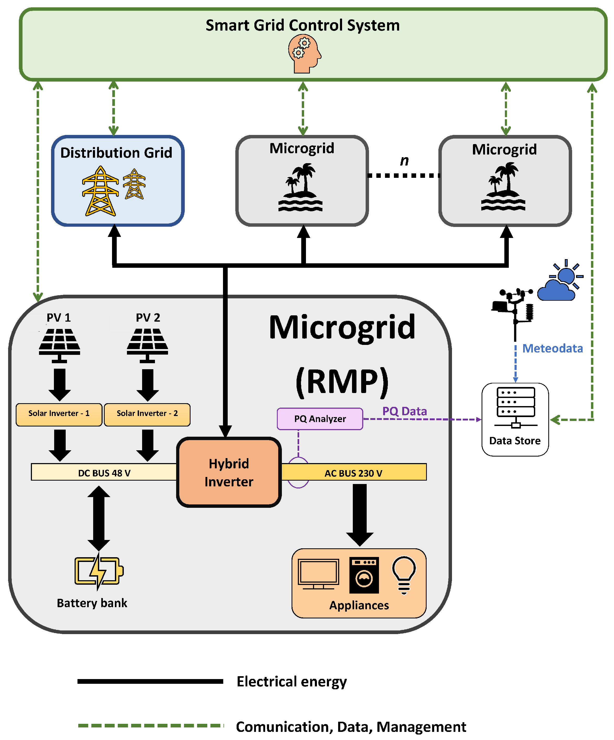
Figure 3.
Location of renewable sources in the physical model of the RMP.
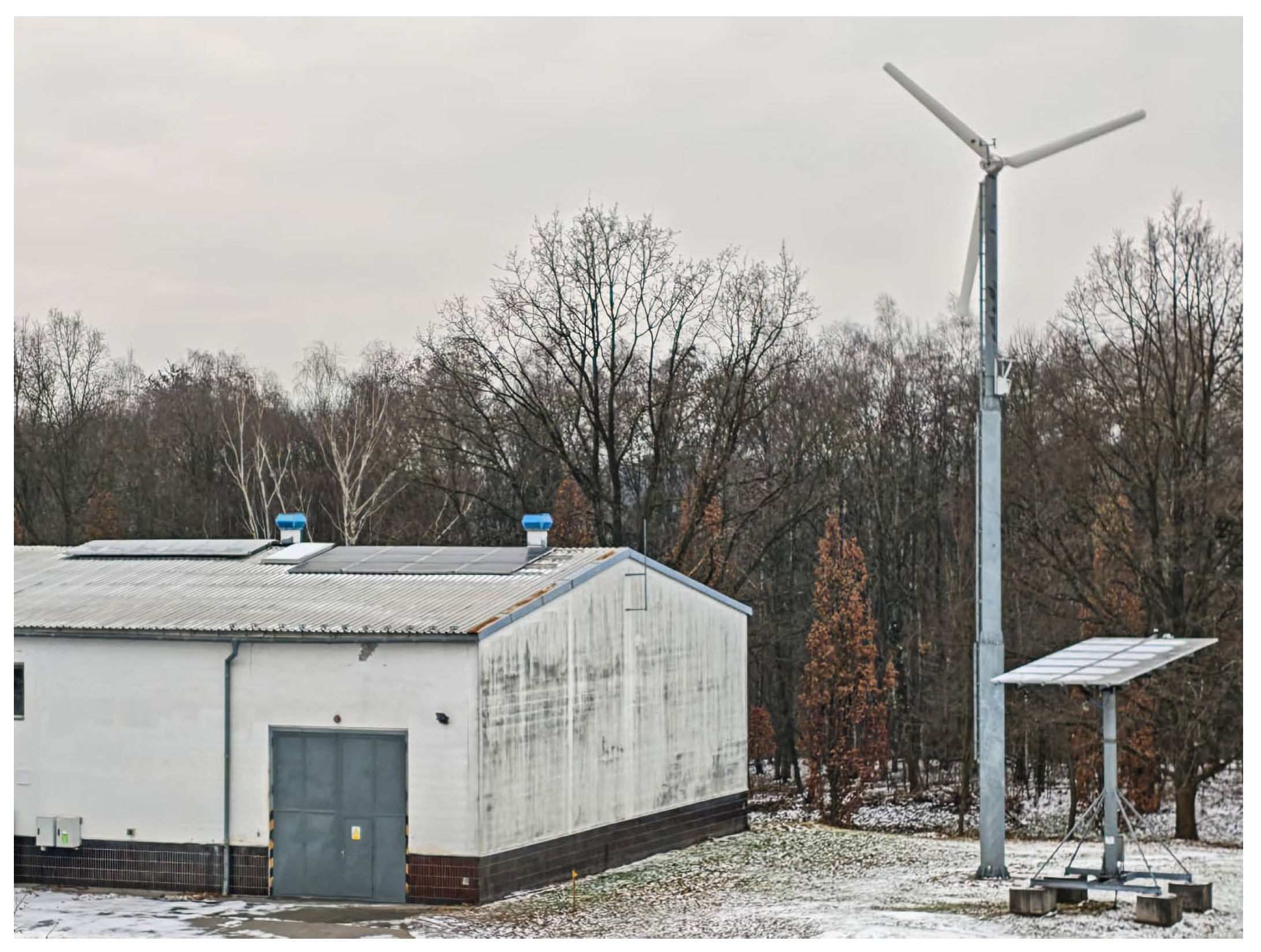
Figure 4.
Hybrid inverter Conext XW+ 8548 and PV inverters Xantrex XW 80 600
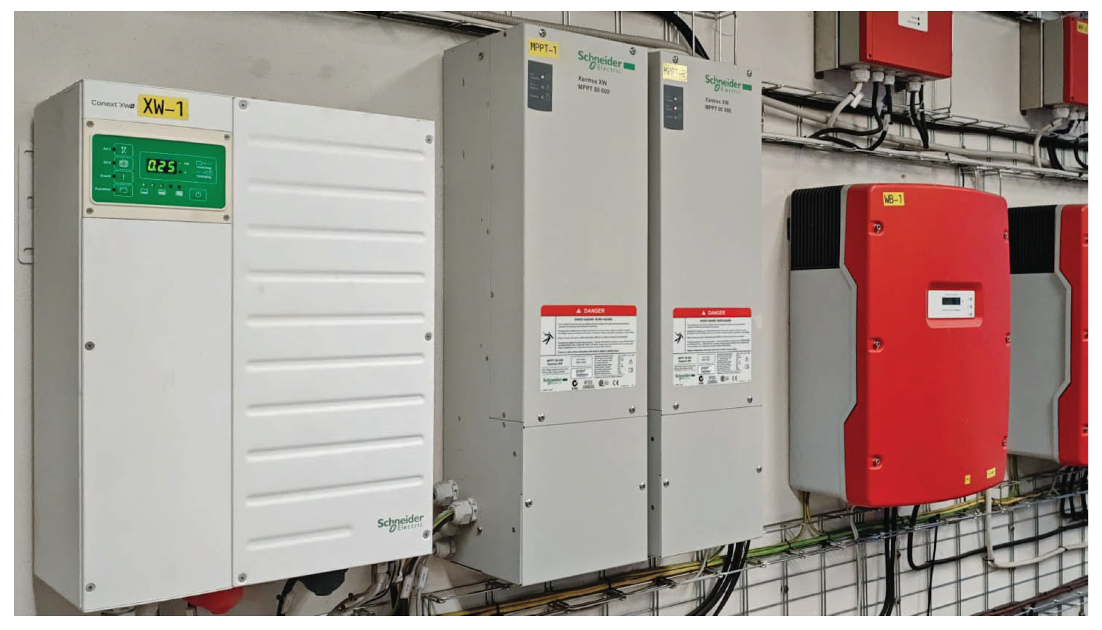
Figure 5.
RMP battery Hawker 12XFC115
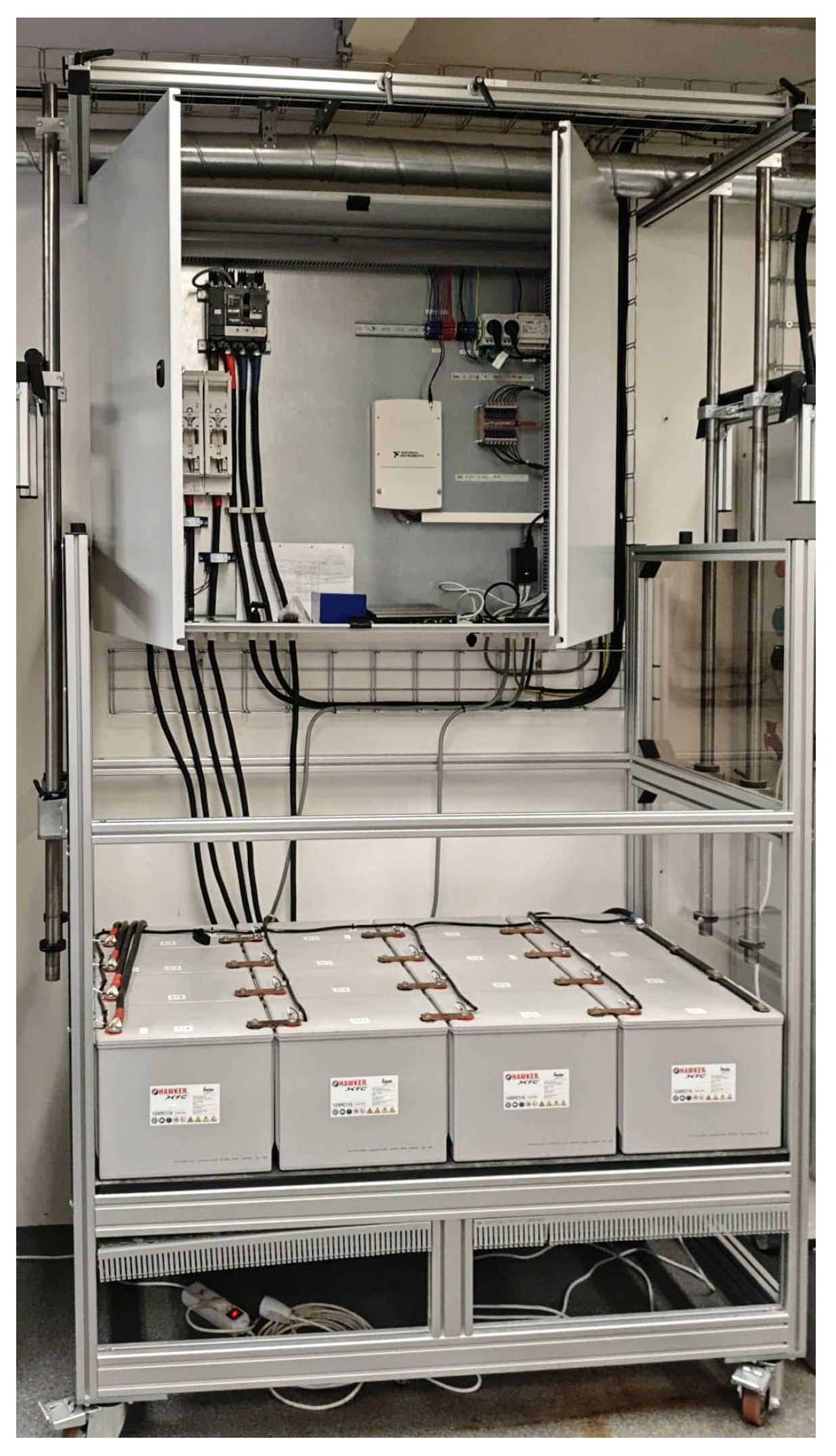
Figure 6.
Support Vector Machine basic principle.
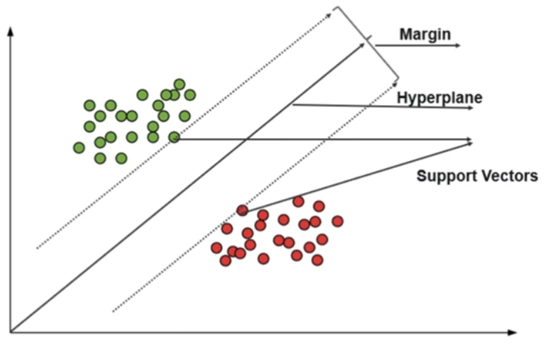
Figure 8.
The LSTM model used in this contribution.
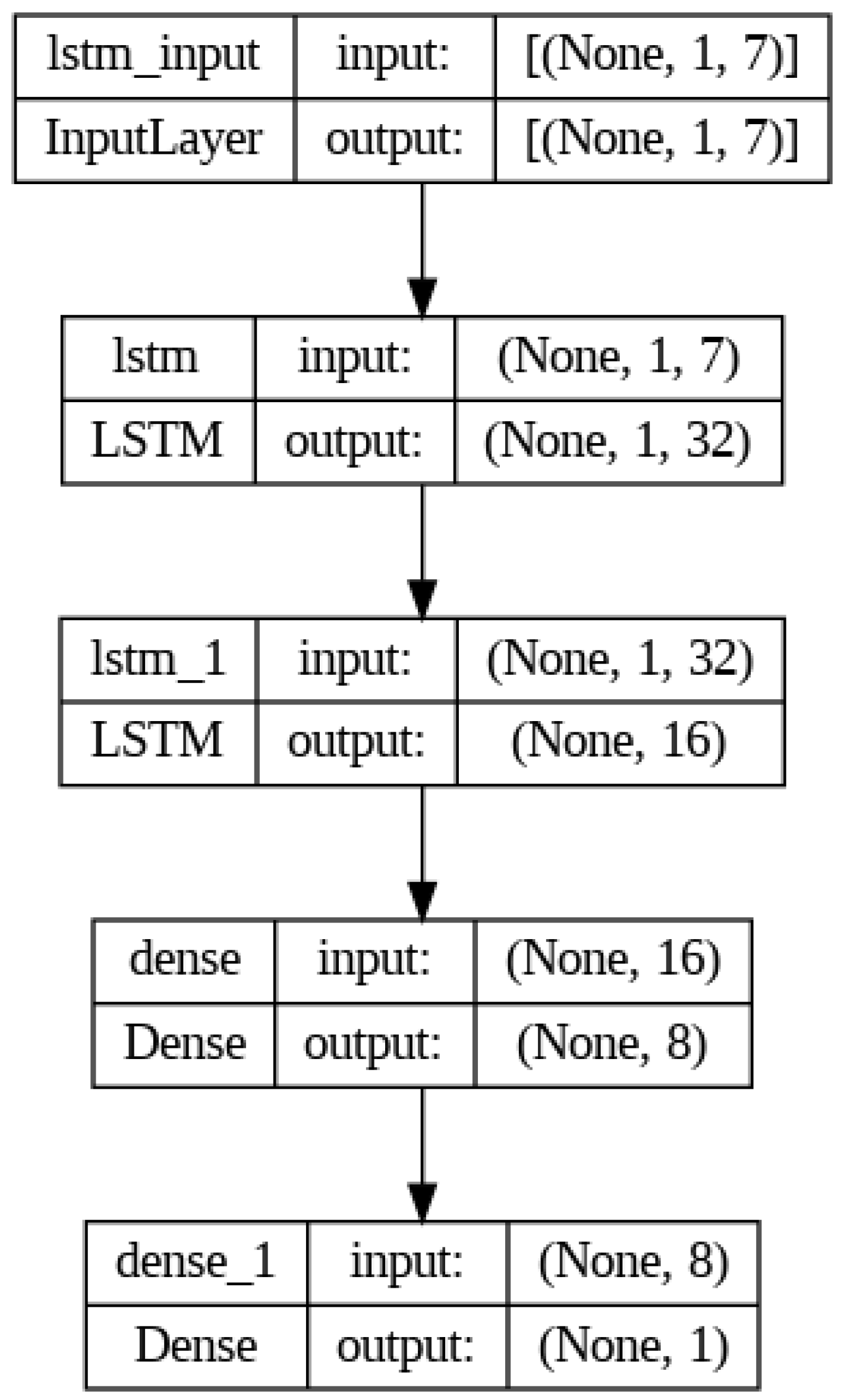
Figure 9.
Scheme of the Proposed Model.
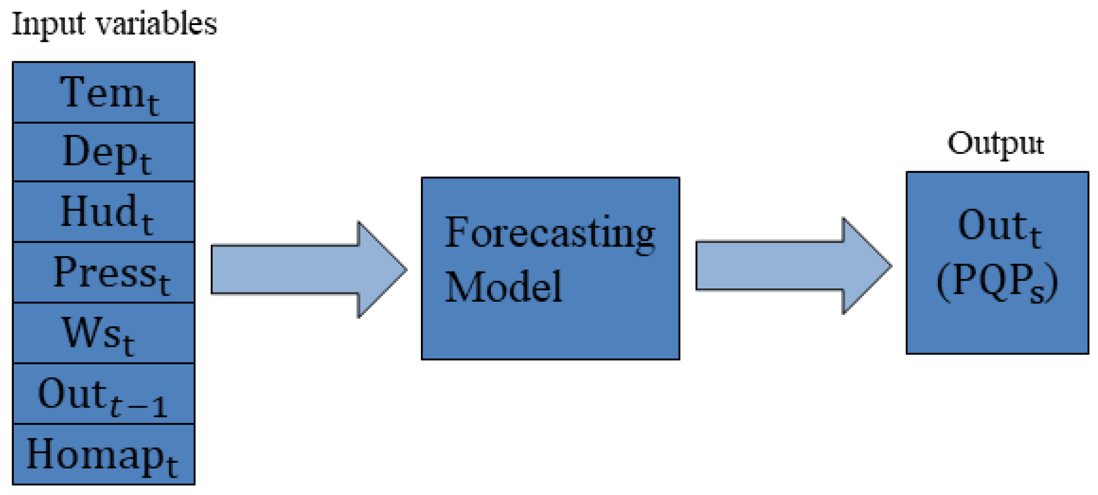
Figure 10.
Comparison of average RMSE for power voltage.
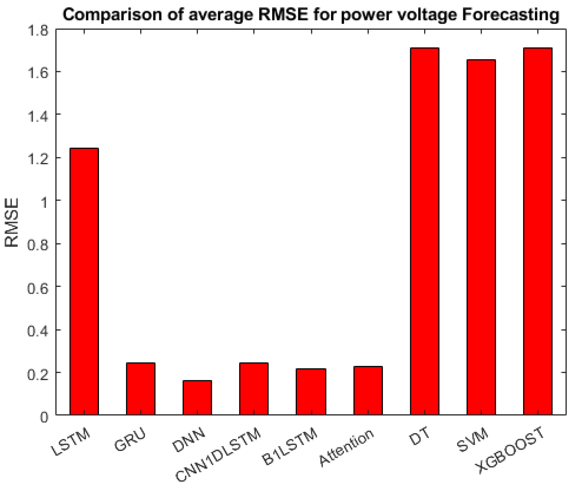
Figure 11.
Comparison of average RMSE for .
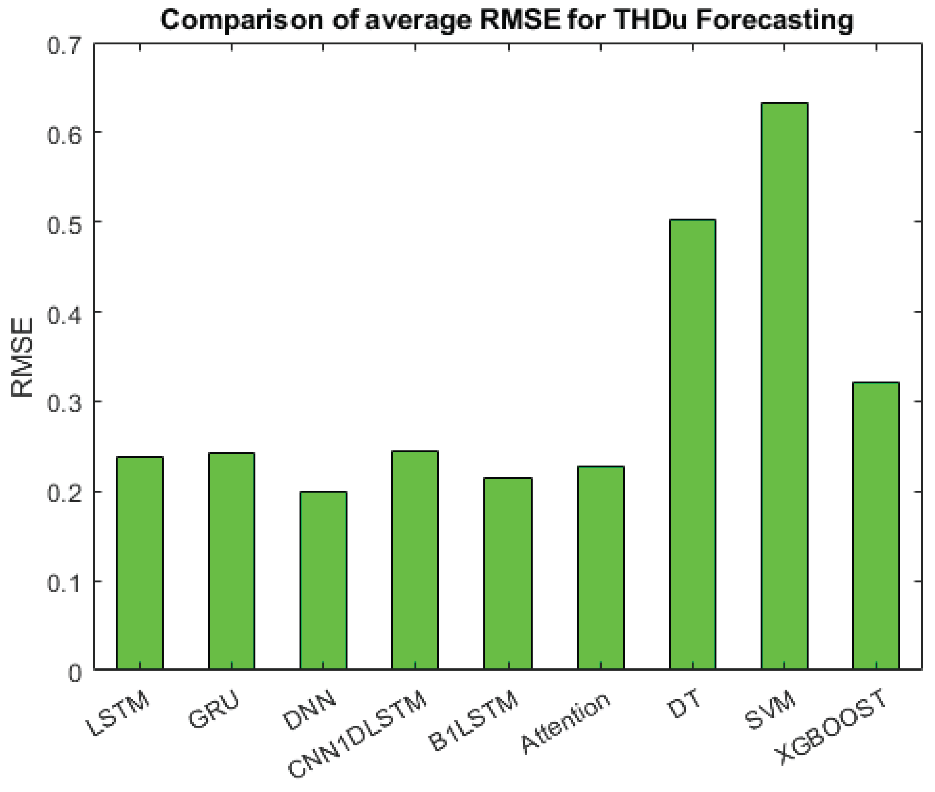
Figure 12.
Comparison of average RMSE for .
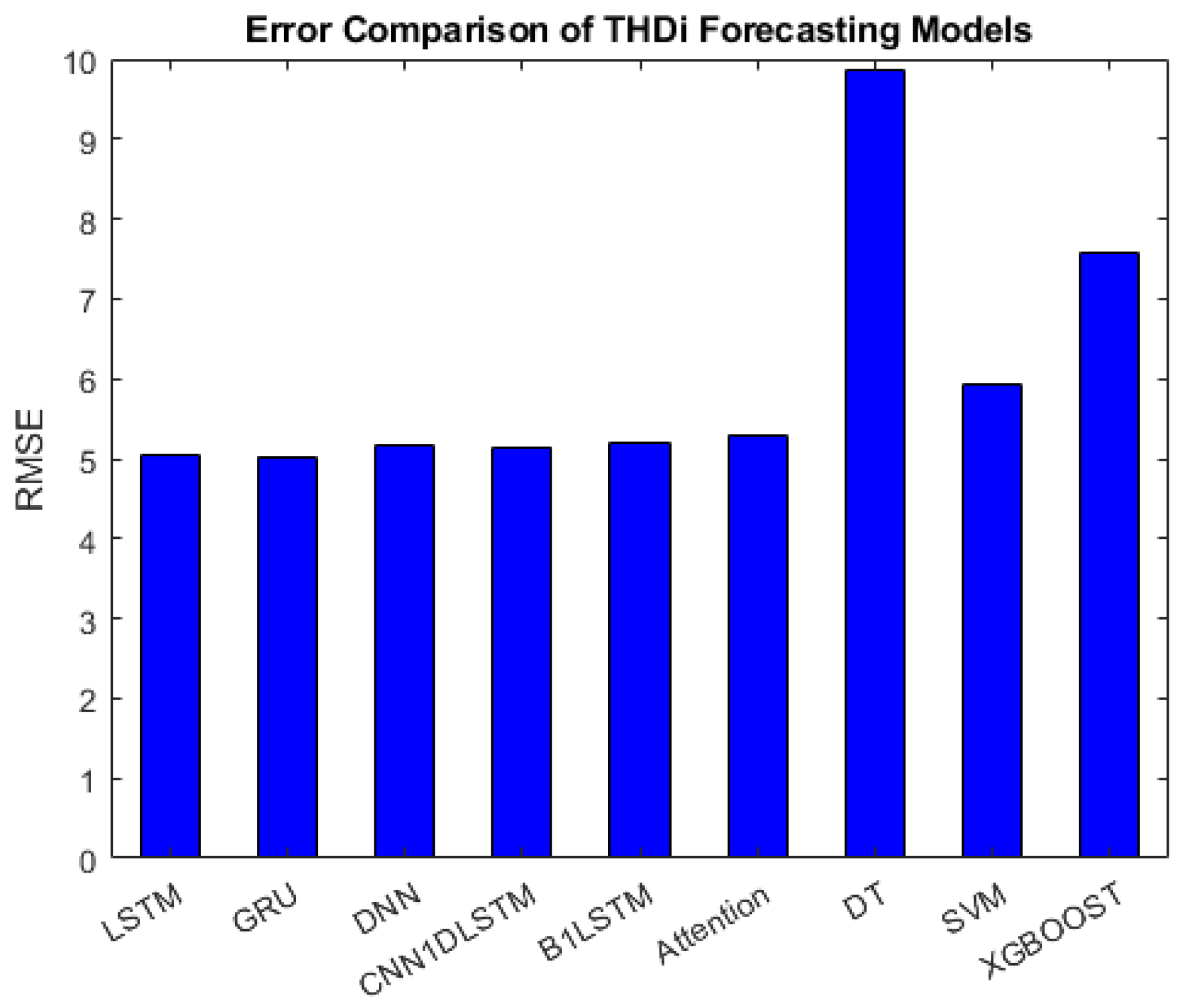
Figure 13.
Comparison of average RMSE for .
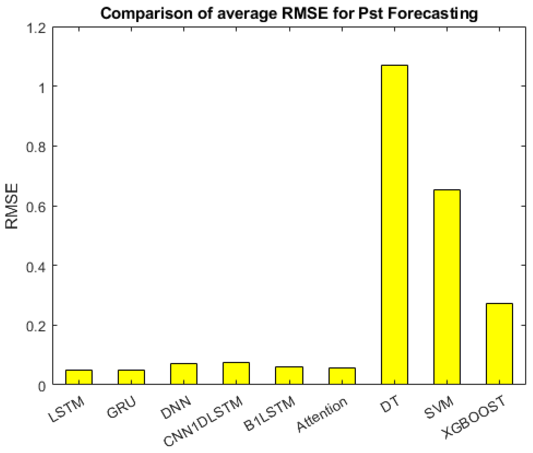
Figure 14.
The radar graph shows the comparison of the RMSE errors of the U, , , and that are achieved by studied models.
Figure 14.
The radar graph shows the comparison of the RMSE errors of the U, , , and that are achieved by studied models.
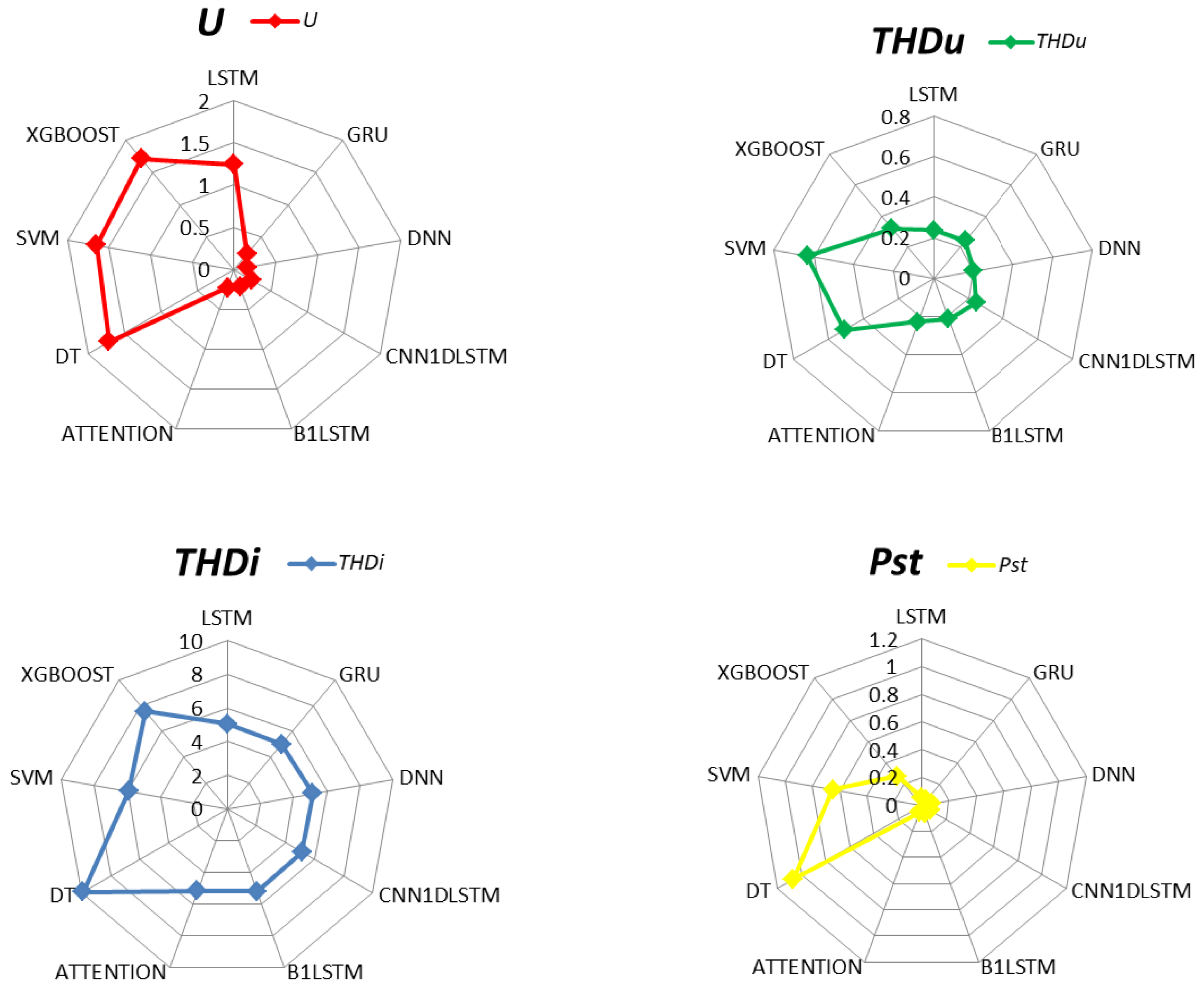
Figure 15.
Time Measurement for one sample.
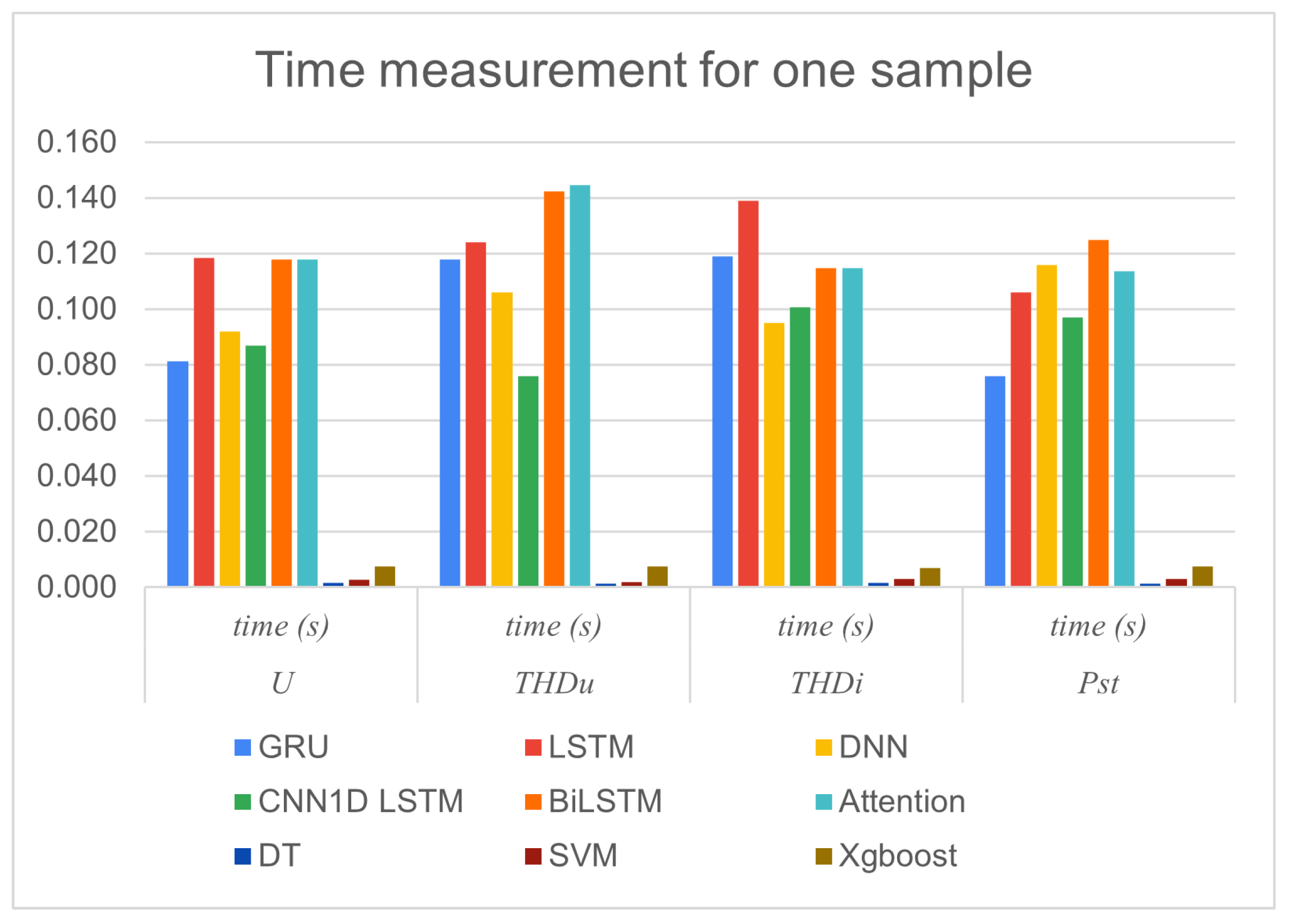
Figure 16.
Memory Measurement for one sample
| Description | Value | Description | Value |
|---|---|---|---|
| Rated continuous power | 6.8 kW | Output voltage AC side | AC |
| Overload (1 min.) | 12.0 kW | No-load consumption | 28 W |
| Overload (5 min.) | 11.0 kW | No-load consumption | <7 W |
| Overload (30 min.) | 8.5 kW | AC side output voltage | 230 V ± 3 % |
| Max. output current (1 min.) | 53.0 A | Output voltage frequency | 50.0 ± 0.1 Hz |
| Continuous Current Load (AC) | 29.5 A | Rated DC side voltage | 48 V DC |
| Maximum efficiency | 95.80 % | DC side operating voltage range | 40-64 V DC |
| Description | Value |
|---|---|
| Maximum PV array no-load voltage | 600 V |
| Maximum inverter output power | 4.8 kW |
| Operating voltage of the PV array | 195–550 V |
| Maximum current from the PV array to the inverter | 23 A |
| Nominal voltage of static battery | 48 V |
| Operating voltage range on static battery | 16–67 V |
| Maximum output current from the inverter | 80 A |
| Maximum inverter efficiency | 95 % |
Table 5.
Input and output variables used in this study
| Variable | Variable description | Input/Output |
|---|---|---|
| Tem | Air temperature | Input |
| Dep | Dew point | Input |
| Hud | Humidity | Input |
| Ws | Wind speed | Input |
| The previous step of the output | Input | |
| Homap | Status of home appliances | Input |
| U | Amplitude of power voltage | Output |
| Voltage total harmonic distortion | Output | |
| Current total harmonic distortion | Output | |
| Short-term flicker severity | Output |
Table 6.
The Forecasting results of power voltage on days 21, 22, 23 of January 2023
| Model | 21st | 22nd | 23rd | Average |
|---|---|---|---|---|
| LSTM | 1.033 | 1.288 | 1.409 | 1.2433 |
| GRU | 0.218 | 0.237 | 0.271 | 0.2420 |
| DNN | 0.097 | 0.219 | 0.1760 | 0.1640 |
| CNN1DLSTM | 0.2116 | 0.230 | 0.289 | 0.2435 |
| B1LSTM | 0.2061 | 0.221 | 0.221 | 0.2160 |
| Attention | 0.2037 | 0.220 | 0.260 | 0.2279 |
| DT | 0.4837 | 0.364 | 4.280 | 1.7090 |
| SVM | 1.588 | 0.820 | 2.557 | 1.6650 |
| xGBoost | 1.543 | 0.913 | 2.676 | 1.7106 |
Table 7.
The Forecasting results of on days 21, 22, 23 of January 2023
| Model | 21st | 22nd | 23rd | Average |
|---|---|---|---|---|
| LSTM | 0.2018 | 0.2187 | 0.2914 | 0.2373 |
| GRU | 0.2181 | 0.2378 | 0.2717 | 0.2425 |
| DNN | 0.2036 | 0.2198 | 0.1765 | 0.1999 |
| CNN1DLSTM | 0.2116 | 0.2303 | 0.2892 | 0.2437 |
| B1LSTM | 0.2061 | 0.2217 | 0.2212 | 0.2148 |
| Attention | 0.2037 | 0.2204 | 0.2605 | 0.2282 |
| DT | 0.3084 | 0.3001 | 0.8999 | 0.5088 |
| SVM | 0.5418 | 0.5766 | 0.7828 | 0.6337 |
| xGBoost | 0.2020 | 0.2821 | 0.4764 | 0.32016 |
Table 8.
The Forecasting results of on days 21, 22, 23 of January 2023
| Model | 21st | 22nd | 23rd | Average |
|---|---|---|---|---|
| LSTM | 3.325 | 6.4134 | 5.3893 | 5.0425 |
| GRU | 3.266 | 6.6723 | 5.1397 | 5.0260 |
| DNN | 3.127 | 6.7659 | 5.5674 | 5.1534 |
| CNN1DLSTM | 3.193 | 6.6438 | 5.5975 | 5.1447 |
| B1LSTM | 3.131 | 6.8060 | 5.6851 | 5.2073 |
| Attention | 3.124 | 6.8641 | 5.9180 | 5.2030 |
| DT | 7.393 | 7.9641 | 14.2588 | 9.8719 |
| SVM | 4.850 | 6.6650 | 6.2401 | 5.9188 |
| xGBoost | 4.966 | 9.4790 | 8.2653 | 7.5701 |
Table 9.
The Forecasting results of on days 21, 22, 23 of January 2023
| Model | 21st | 22nd | 23rd | Average |
|---|---|---|---|---|
| LSTM | 0.0417 | 0.05802 | 0.0524 | 0.050706 |
| GRU | 0.0493 | 0.05116 | 0.0516 | 0.050686 |
| DNN | 0.0772 | 0.06806 | 0.0654 | 0.07022 |
| CNN1DLSTM | 0.0679 | 0.07342 | 0.0797 | 0.07367 |
| B1LSTM | 0.0537 | 0.05752 | 0.0659 | 0.05904 |
| Attention | 0.0264 | 0.03696 | 0.0402 | 0.057544 |
| DT | 1.2534 | 1.1399 | 0.8128 | 1.06870 |
| SVM | 0.6269 | 0.6418 | 0.6872 | 0.651966 |
| xGBoost | 0.4142 | 0.0748 | 0.3257 | 0.271566 |
Table 10.
Computational Complexity: computation time (seconds) and Memory (KB)
| Model | U | |||||||
|---|---|---|---|---|---|---|---|---|
| Time | Memory | Time | Memory | Time | Memory | Time | Memory | |
| LSTM | 0.119 | 272.735 | 0.124 | 276.660 | 0.139 | 214.421 | 0.106 | 267.585 |
| GRU | 0.081 | 217.929 | 0.118 | 286.622 | 0.119 | 202.597 | 0.076 | 136.591 |
| DNN | 0.092 | 757.564 | 0.106 | 311.945 | 0.095 | 200.623 | 0.116 | 364.393 |
| CNN1DLSTM | 0.087 | 335.571 | 0.076 | 201.260 | 0.101 | 196.585 | 0.097 | 203.398 |
| B1LSTM | 0.118 | 256.283 | 0.142 | 278.575 | 0.115 | 201.233 | 0.125 | 258.450 |
| Attention | 0.118 | 207.071 | 0.145 | 294.189 | 0.115 | 202.120 | 0.114 | 199.856 |
| DT | 0.002 | 108.168 | 0.002 | 111.078 | 0.002 | 91.957 | 0.001 | 106.699 |
| SVM | 0.003 | 108.376 | 0.002 | 78.504 | 0.003 | 96.666 | 0.003 | 107.882 |
| xGBoost | 0.008 | 152.049 | 0.008 | 159.943 | 0.007 | 149.142 | 0.008 | 154.691 |
Disclaimer/Publisher’s Note: The statements, opinions and data contained in all publications are solely those of the individual author(s) and contributor(s) and not of MDPI and/or the editor(s). MDPI and/or the editor(s) disclaim responsibility for any injury to people or property resulting from any ideas, methods, instructions or products referred to in the content. |
© 2026 by the authors. Licensee MDPI, Basel, Switzerland. This article is an open access article distributed under the terms and conditions of the Creative Commons Attribution (CC BY) license (http://creativecommons.org/licenses/by/4.0/).
Copyright: This open access article is published under a Creative Commons CC BY 4.0 license, which permit the free download, distribution, and reuse, provided that the author and preprint are cited in any reuse.


