
Submitted:
19 February 2026
Posted:
19 February 2026
You are already at the latest version
Abstract
Spatial light field metrics such as mean cylindrical illuminance provide essential information for qualitative lighting evaluation, yet they remain far less common in practice than horizontal illuminance. To address this gap, we present a multi-sensor prototype that simultaneously measures horizontal illuminance Eh and approximates mean cylindrical illuminance Ez from a set of vertical illuminances uniformly spaced around a cylindrical surface. The device uses a flexible PCB wrapped around a support barrel and an inertial and magnetic measurement unit for orientation tracking. The measurements enable direct calculation of the modelling factor defined in the technical standard EN 12 464 and visualization of directional light distribution using polar plots and illuminance solid. Results show that the prototype approximates mean cylindrical illuminance with high accuracy while preserving directional information, allowing the illuminance solid to be decomposed into vector and symmetric components. Compared with conventional approximation methods, the proposed multi-sensor approach reduces spatial error and yields richer data for lighting analysis. These findings indicate that multi-sensor systems can bridge the gap between theoretical spatial metrics and practical photometry and support the improved modelling evaluation and integration of qualitative lighting parameters into routine workflows.
Keywords:
illuminance measurements
; spatial illuminance characteristics
; mean cylindrical illuminance
; modelling factor
; illuminance solid
1. Introduction
Research on scalar and vector properties of the light field dates back to 1885 when Weber introduced luminance and illuminance distribution solid and made early attempts to define average spherical illumination [1], now known as scalar illuminance [2]. Gershun’s 1936 work The Light Field [3] introduced the illuminance solid as a vector metric of qualitative properties of lighting as a fundamental description of the light field in the given point. Subsequently, hemi-scalar illuminance was formulated as a related scalar metric [4], followed by mean cylindrical illuminance in 1965 [5]. Lynes et al. extended Gershun's paper in 1966 with the concept of the flow of light that delivered the subject to a broader audience [6]. Cuttle [7] and Lynes [8,9] later developed the concept of the flow of light and multiple measurement methods of the flow of light were proposed [10], including Bunsen's grease spot photometer [11,12].
In 1997 Cuttle proposed cubic illuminance [13] as a spatial distribution metric aligned with the Cartesian coordinate system and described its calculation and measurement. Parallel research by prof. Habel at Czech Technical University [14,15] explored cubic illuminance in 1993, although it was not published in English. Vector and symmetric components were explained in Cuttle's books [16,17] as the two major components of illumination solid. Later studies by Cuttle [18], Straka [19], Mangkuto [20], and Xia et al. [21,22] showed that cubic and planar illuminances can be approximated by cylindrical or scalar distributions with different levels of uncertainty. Mangkuto [23,24] and Xia et al. [25,26] compared several cubic to scalar approximation methods across many lighting situations and mapped their error with practical recommendations.
Despite extensive research, spatial metrics such as cubic, scalar, and cylindrical illuminance remain rarely used in routine photometry. Most technical standards prioritize horizontal illuminance for indoor workplaces and outdoor public areas, while spatial metrics, such as scalar or cylindrical illuminance, are usually mentioned only as recommendations [27,28,29,30]. The updated CEN standard EN 12 464 [31] highlights mean cylindrical illuminance Ez and the modelling factor, defined as the ratio of mean cylindrical to horizontal illuminance. Recommended modelling factor values for indoor environments are 0.3-0.6 [32], excluding cases where daylight contributes significantly. Values below 0.3 indicate predominance of horizontal illuminance and can produce undesirable facial shadowing [33].
At present, evaluating cylindrical illuminance in line with new technical standard recommendations [31] typically relies on calculations on a digital model of the lighting installation. Commercial photometers capable of measuring spatial distributions are rare. Cylindrical, semi-cylindrical, scalar, and semi-scalar photometer heads exist only as specialized accessories for portable light meters [35,36]. Devices for cubic illuminance are not commercially available and the measurement is either done by six separate illuminance meters or by rotating a single receiver in six directions of the cube [16,17,18,21,22]. Consequently, modelling factor measurements usually require two instruments: one for horizontal illuminance and another for cylindrical illuminance.
2. Scalar and Vector Approach to Cylindrical Illuminance
Scalar cylindrical illuminance in the real environment can be measured directly with a single detector with a specialized photometric head [35,36], see Figure 1 a). A close cylindrical illuminance approximation can be obtained by taking multiple measurements with a planar photometric head a with cosine corrector oriented to various directions around the vertical axis (Figure 1 c), or by using a single head fitted with several detectors as in Figure 1 b). By analogy to the last case, scalar illuminance can be derived from repeated single-plane illuminance En measurements taken from multiple directions at point P or by axial rotation of a multi-sensor head. The mean value of an indefinite number of such illuminances pointing to point P in the direction of the single plane equals mean cylindrical illuminance Ez [5].
The simplest approximation of cylindrical illuminance uses four planar illuminances aimed toward the faces of an imaginary cube with greater spatial error significance (Figure 1 c). The spatial error of the approximation can be further lowered by increasing the number of illuminance directions on the cylindrical surface, where in case described in Figure 1 b), the mean spatial error for Ez approximation from 36 illuminances falls below 0.2 % [37]. Figure 2 shows the error as a function of sensor count. The process of selecting the number of sensors is also described in detail in [37]. 36 sensors provide a directional measurement step of 10 angular degrees. The residual approximation error arises from the cosine response of each detector, since the sensor output is weighted by the cosine of the incidence angle.
Quality factors for a total characteristic of the illuminance meter performance are part of EN standard 13032-1 [38], yet spatial distribution characteristics deviation limits are not covered. German standard DIN 5032-7:2017 [39] specified class limits for illuminance meters, including scalar, cylindrical, semi-cylindrical, and semi-scalar illuminance spatial response for all four accuracy classes (L, A, B, C) [39]. The most accurate photometer class for in-field illuminance measurement (A) defines allowed cosine response deviation for standard illuminance < 1.5 %, cylindrical illuminance < 5 %, and scalar illuminance < 10 % [39]. The spatial error of the prototype should therefore not contribute significantly to increasing measurement uncertainties above the specified limits.
3. Multi-Sensor Measurement Device Prototype
The properties mentioned above motivated authors of this article to develop a single multi-sensor prototype that simultaneously measures horizontal illuminance Eh and approximates mean cylindrical illuminance Ez as from the average of vertical illuminances measured by illuminance sensors uniformly distributed around a cylindrical surface (see Figure 3).
The device also estimates the magnitude and direction of the vector component and directly computes the modelling factor specified in EN 12464 [31].
Compared to previous prototypes [37], the cylindrical sensor assembly consists of five PCB boards. Two flexible PCBs carrying the vertical sensors are wrapped around a support cylindrical barrel and connected to a main PCB, which contains the main logic, power management, and data-acquisition stage, including ADCs and multiplexers. The horizontal illuminance sensor, status LED and IMMU are located on the top PCB. A user interface LCD and two buttons are situated on the horizontal PCB. The device supports battery-powered operation and USB data acquisition. The sensor topology follows Figure 4 [37].
As illustrated in Figure 5, the SFH 5711 sensor array signals Iout are multiplexed, converted to voltage Vout across a load resistor Rl, and low-pass filtered (f) by the ADS131M04 AD converter. The number of ADC channels matches the number of multiplexers. The AD converter outputs are acquired by the MCU over SPI bus as digital data frames.
Real-time access to 36 individual vertical illuminances En on the cylindrical surface at 10 degrees steps (Figure 6) enables approximate evaluation of cylindrical illuminance evaluations consistent with the approaches of Gershun [3] and Lynes [40]. Semi-cylindrical illuminance and opposite illuminances can be obtained for any azimuth without moving the device.
An onboard inertial–magnetic measurement unit (IMMU) [41] provides approximate information about the horizontal plane level (spirit level) and heading off the device with respect to magnetic north (compass). Knowing the absolute device's orientation offers the theoretical option of reconstruction the full illuminance solid by rotating the cylinder head about the horizontal axis.
After final assembly, the IMMU Bosch BMX160 is calibrated by leveling the device to trigger an internal FOC command for gyroscope bias and rotating it through PJRC MotionCal to compensate for housing interference with a 3×3 magnetometer mapping matrix. This yields a heading accuracy of ±1° to ±2.5° and a gyroscope offset of ±0.1°/s. The accuracy is expected to drift over time due to temperature fluctuations, sensor aging or external field effects.
4. Results
The prototype simultaneously acquires 36 vertical illuminances En and horizontal illuminance Eh, enabling direct computation of the modelling factor [31] from a single measurement. The single vertical illuminance En values can be plotted in polar form (Figure 7) and connected to form a continuous outline (Figure 8).
A concise description of the light field at a point is given by a cross-section of the illuminance solid, constructed from illuminances En measured in various directions (vectors) [3]. The illuminance solid is a three-dimensional surface whose radius in any direction equals the illuminance En in that direction. Considering a two-dimensional section, the relevant illuminances lie in single plane around point P (see Figure 8). Vertical illuminances sampled on a cylindrical surface with axis perpendicular that plane are measured by the multi-sensor cylindrical device prototype, and their mean value corresponds to mean cylindrical illuminance Ez.
The illuminance solid (blue line in Figure 8) comprises two principal components: a vector component (red) and a symmetric component (light blue). The vector component’s magnitude and direction correspond to the illuminance vector (red arrow) [3]. The symmetric component can be further divided into its diffuse and non-diffuse symmetric components [16,17]. The two-dimensional illumination solid is considered on a horizontal plane, i.e., in all horizontal directions from point P. The vector component indicates a dominant light source direction, whereas the diffuse component represents ambient light.
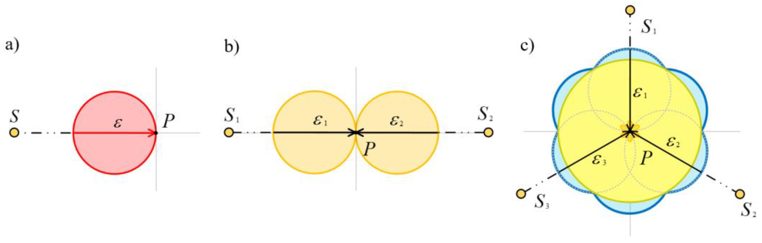
Simulation examples for a multi-sensor at point P illustrate typical cross-sections: an environment with single point light source S (Figure 9a; dominant vector component), two opposite point light sources S1 and S2 (Figure 9b; non-diffusive symmetric component only), and three evenly spaced point light sources S1 , S2 and S3 (Figure 9c; largely symmetric and diffusive component).
If light arrive uniformly from all horizontal directions, the two-dimensional cross-section of illumination solid approaches a circle centered at the location of the multi-sensor (point P). In such an environment, objects do not cast any shadows, and it can be very difficult to distinguish the surface structure of objects (e.g., facial features). Conversely, if the multi-sensor is located in an environment with a dominant light source in one horizontal direction, the vector component (red colored in the Figure 8 and Figure 9) of illumination solid grows and the modeling factor increases. A single horizontal point light source (Figure 9 a) maximizes the modeling factor and produces sharp shadows. Conversely, with a single vertical point light source and neglible horizontal flow of light, the modeling factor approaches its minimum. Both single point light source extremes (either vertical or horizontal) fall outside the recommended range of modeling factor.
5. Discussion
The results demonstrate the feasibility of a multi-sensor approach for cylindrical illuminance measurements while preserving directional information. This is consistent with previous theoretical frameworks by Gershun [3,4] and Lynes [2,8,9], which emphasize vector and symmetric components as fundamental descriptors of illumination. Although standards such as EN 12464 [31] recognize cylindrical illuminance for modelling evaluation, practical implementation has been limited by a lack of practical instruments. Author’s prototype addresses this gap by enabling simultaneous measurement of Eh and Ez and real-time modelling factor computing. Compared with rotational or four-direction approximations, the 36-sensor configuration significantly reduces spatial error from more than 10 % (4-sensor configuration) to less than 0.2 %. These functions are relevant to workplace lighting, architectural design, and ergonomic assessment, where modelling quality influences visual comfort and perception. Future research should focus on metrological validation against reference-class photometers, algorithmic processing for automated vector decomposition, and sensor topology optimization for cost-effective production [42]. Integrating such devices into routine photometry could accelerate adoption of spatial metrics and close the gap between standards requirements and practical lighting evaluation.
6. Conclusions
The research confirms that spatial illuminance metrics, particularly cylindrical illuminance, play a crucial role in qualitative lighting evaluation, yet their practical implementation has been hindered by technical limitations. The proposed multi-sensor prototype offers accurate mean cylindrical illuminance approximation and directional light field analysis in a single measurement. This innovation aligns with normative modelling factor requirements and offers additional insights into illumination vector properties. To achieve broader adoption, further development is needed to improve measurement accuracy and improve device complexity. Ultimately, integrating such solutions into standard lighting assessment practice can significantly enhance visual comfort and modelling quality in architectural and workplace environments.
Author Contributions
Conceptualization, M.B.; methodology, P.Z.; software, M.K.; validation, P.Z. and M.B.; formal analysis, M.K.; investigation, M.K.; resources, M.K.; data curation, M.K.; writing—original draft preparation, M.K.; writing—review and editing, M.B.; visualization, M.K.; supervision, P.Z.; project administration, M.B.; funding acquisition, M.B. All authors have read and agreed to the published version of the manuscript.
Funding
This research was funded by Czech Technical University in Prague, grant number SGS23/167/OHK3/3T/13.
Institutional Review Board Statement
Not applicable.
Informed Consent Statement
Not applicable.
Data Availability Statement
Dataset available on request from the authors.
Conflicts of Interest
The authors declare no conflicts of interest.
References
- Weber, L. Intensitätsmessungen des diffussen Tageslichtes. Ann d. Phys, 1885, 262 (11), 374-389. [CrossRef]
- Lynes, J.A. Cylindrical or scalar illumination? Lighting Research & Technology, 1970, 2(4), 265-266. [CrossRef]
- Gershun, A., The Light Field. Unify Technical Press, 1936, English translation by Moon, P. and Timoschenko G. Journal of Mathematical Physics, 1939, 18, 51–151.
- Gershun, A. Characteristics of Conditions of Illumination, Trans. Optical Institute, 1931, 59, 6.
- Epaneshnikov, K.M.; Sidorova, T.N. The evaluation of light saturation of rooms of public buildings. Svetloteknika, 1965, 11, 11.
- Lynes, J.A.; Burt, W.; Jackson, G.; Cuttle, C. The Flow of Light into Buildings. Lighting Research & Technology, 1966, 31(3), 65-91. [CrossRef]
- Cuttle, C. Lighting patterns and the flow of light. Lighting Research & Technology, 1971, 3(3), 171-189. [CrossRef]
- Linnes, J.A. Estimating scalar illuminance. Lighting Research & Technology, 1975, 7(2), 142-143. [CrossRef]
- Lynes, J.A. The luminaire domain and the flow of light. Lighting Research & Technology, 1975, 7(4), 242-250. [CrossRef]
- Fuller, M., Upton, M., & Whalen, J. The photometry of the flow of light. Lighting Research & Technology, 1971, 3(4), 282-284. [CrossRef]
- Dale, N., Broadbridge, J., & Crowther, P. Measuring the direction of the flow of light. Lighting Research & Technology, 1972, 4(1), 43-44. [CrossRef]
- Lewis, D.M. Bunsen's Photometer. Nature, 1889, 40 (174). [CrossRef]
- Cuttle, C. Cubic illumination. Lighting Research & Technology, 1997, 29(1), 1-14. [CrossRef]
- Habel et al. Average Cubic Illumination, In 9th International Conference on Energy Effective and Ecologically Beneficial Lighting "Lighting '93", Varna, Bulgaria, 1993.
- Habel et al. Svetlo a osvetlovani; FCC Public: Prague, Czech Republic, 2013. ISBN 978-80-86534-21-3.
- Cuttle, C. Lighting by Design; Elsevier Science: Burlington, USA, 2003. ISBN: 0-7506-5130-X.
- Cuttle, C. Lighting design: A perception-based approach. Routledge, 2015.
- Cuttle, C. Research Note: A practical approach to cubic illuminance measurement. Lighting Research & Technology, 2014, 46(1), 31-34. [CrossRef]
- Straka, T. Quality assessment of lighting systems, Dissertation Thesis, 2001. Czech Technical Unversity in Prague, Departement of El. Power Engineering. Thesis supervisor: J. Habel.
- Mangkuto, R. Uncertainty Analysis of Cylindrical Illuminance Approximation. LEUKOS, 2019, 16. 1-12. [CrossRef]
- Xia, L., Pont, S., & Heynderickx, I. Light diffuseness metric Part 1: Theory. Lighting Research & Technology, 2017, 49(4), 411-427. [CrossRef]
- Xia, L., Pont, S., & Heynderickx, I. Light diffuseness metric, Part 2: Describing, measuring and visualising the light flow and diffuseness in three-dimensional spaces. Lighting Research & Technology, 2017, 49(4), 428-445. [CrossRef]
- Mangkuto, R. A comparison of three approaches for determining scalar illuminance from cubic illuminance data. Lighting Research & Technology, 2019, 51(4), 625-641. [CrossRef]
- Mangkuto, R. Research note: The accuracy of the mean spherical semi-cubic illuminance approach for determining scalar illuminance. Lighting Research & Technology, 2019, 52(1), 151-158. [CrossRef]
- Xia, L., Xiao, N., Liu, X., Zhang, T., Xu, R., & Li, F. Determining scalar illuminance from cubic illuminance data – Part 1: Error tracing. Lighting Research & Technology, 2022, 55(1). [CrossRef]
- Xia, L., Gu, Y., Liu, X., Zhang, T., & Xu, R. Determining scalar illuminance from cubic illuminance data. Part 2: Tests in real lighting environments and an approach to improve its accuracy. Lighting Research & Technology, 2022, 55(1). [CrossRef]
- Council of Standards Australia. Interior and workplace lighting General principles and recommendations. AS 1680 Sydney: 2006.
- The British Standards Institution. Lighting for buildings. BS 8206. [CrossRef]
- Japanese Standards Association. Lighting for sports halls. JIS Z 9122.
- Illuminating Engineering Society. Recommended Practice: Lighting Office Spaces. ANSI/IES RP-1:2024.
- European Committee for Standardisation (CEN). Light and Lighting: Lighting for Workplaces: Indoor Workplaces. EN 12464-1 2021. Brussels: CEN, 2021.
- Bean, A. Modelling indicators for combined side and overhead lighting systems. Lighting Research & Technology, 1978, 10(4), 199-202.
- Boyce, P., Brandston, H., & Cuttle, C. Indoor lighting standards and their role in lighting practice. Lighting Research & Technology, 2022, 54(7), 730-744. [CrossRef]
- Gooding, P., Hunt, D., & Cockram, A. Instrument for the direct measurement of mean cylindrical illuminance. Lighting Research & Technology, 1976, 8(4), 225-229.
- PRC krochmann (http://www.prc-krochmann.eu/Produkte/photometerkoepfe/).
- LMT Lichtmessetechnik Berlin (https://www.lmt.de/lmt-photometer-heads/).
- M. Kozlok and P. Žák, "Photodetectors for cylindrical illuminance sensor", 2020 21st International Scientific Conference on Electric Power Engineering (EPE), 2020, pp. 1-5. [CrossRef]
- European Committee for Standardisation (CEN). Light and Lighting: Measurement and presentation of photometric data of lamps and luminaires - Part 1: Measurement and file format. EN 13032-1:2004+A1:2012. Brussels: CEN, 2004.
- Deutsches Institut für Normung. Photometry - Part 7: Classification of illuminance meters and luminance meters. DIN 5032-7:2017. [CrossRef]
- Lynes, J. Fourier components of cylindrical illuminance. Lighting Research & Technology, 2019, 51(8), 1224-1236. [CrossRef]
- Zmitri, M., Fourati, H., & Vuillerme, N. Human Activities and Postures Recognition: From Inertial Measurements to Quaternion-Based Approaches. Sensors (Basel, Switzerland), 2019, 19(19). [CrossRef]
- R. Hrbac, V. Kolar, T. Novak and M. Bartłomiejczyk, " Prototype of a low-cost luxmeter with wide measuring range designed for railway stations dynamic lighting systems ", 2014 15th International Scientific Conference on Electric Power Engineering (EPE), 2014. [CrossRef]
Figure 1.
Graphical representation of a) scalar cylindrical illuminance, b) cylindrical illuminance measured from 36 single detector illuminances, c) cylindrical illuminance from 4 single detector illuminances. Above EN directions, below three-dimensional shape of spatial sensitivity.
Figure 1.
Graphical representation of a) scalar cylindrical illuminance, b) cylindrical illuminance measured from 36 single detector illuminances, c) cylindrical illuminance from 4 single detector illuminances. Above EN directions, below three-dimensional shape of spatial sensitivity.
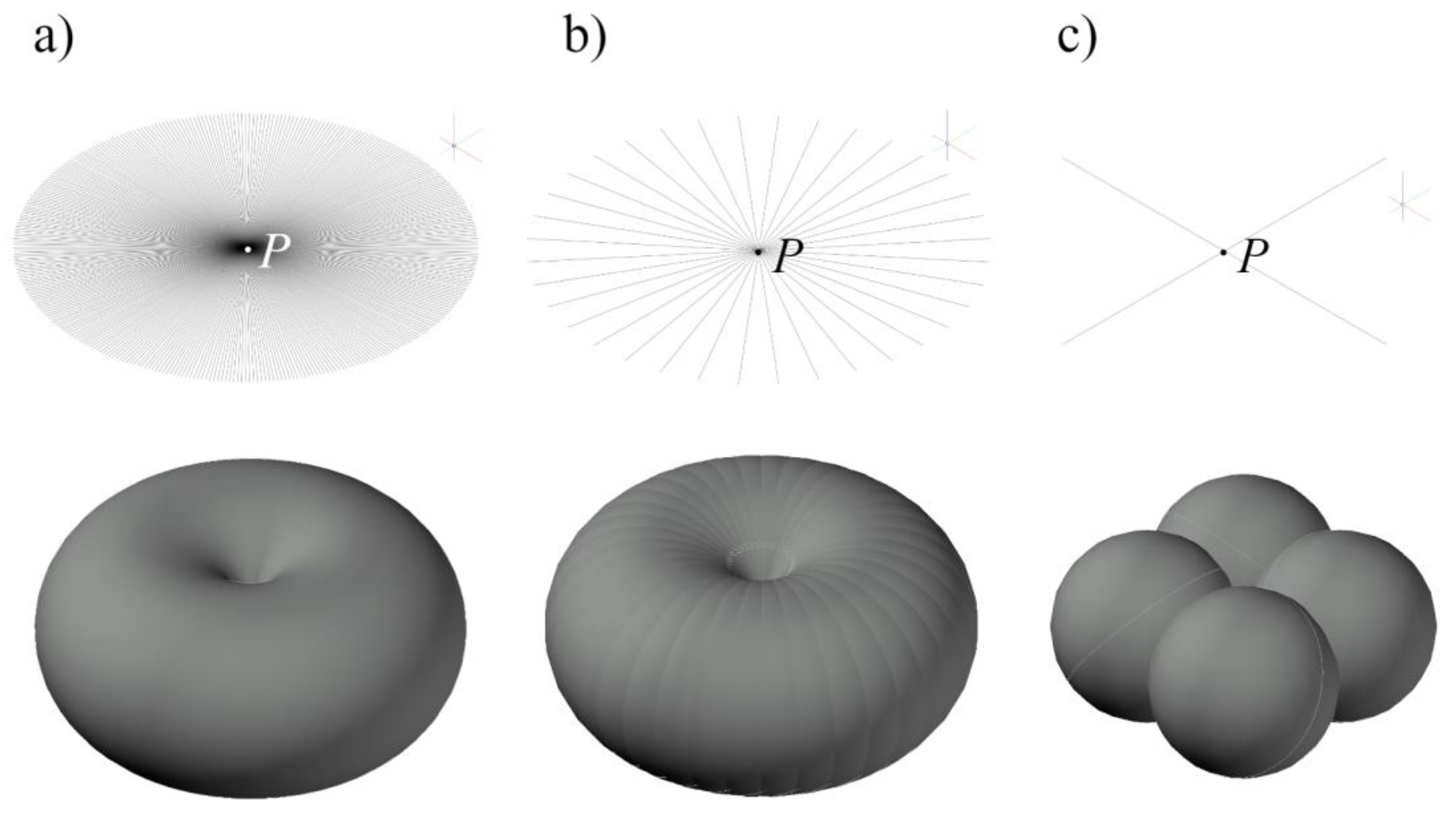
Figure 2.
The dependence of spatial error on the number of sensors. Min Error is the error of illuminance approximation in the direction of the normal to the sensor and Max Error is the error of illuminance approximation in the direction of the border between two sensors.
Figure 2.
The dependence of spatial error on the number of sensors. Min Error is the error of illuminance approximation in the direction of the normal to the sensor and Max Error is the error of illuminance approximation in the direction of the border between two sensors.
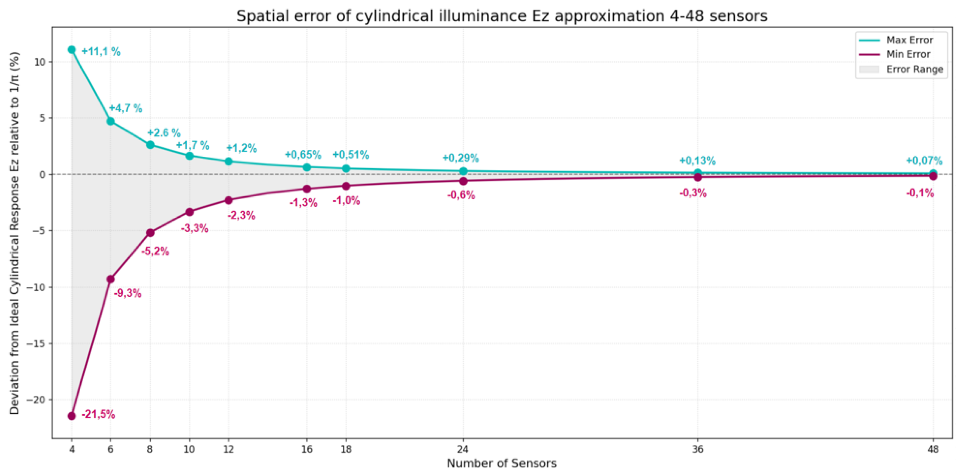
Figure 3.
Proposed construction of multi-sensor cylindrical illuminance sensor, drawing and model render.
Figure 3.
Proposed construction of multi-sensor cylindrical illuminance sensor, drawing and model render.
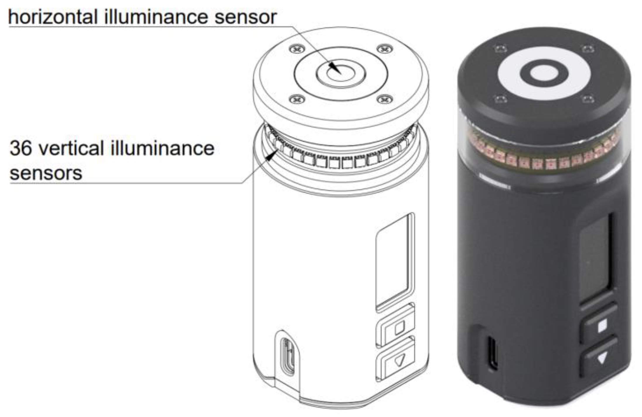
Figure 4.
The topology of cylindrical multi-sensor device prototype [37].
Figure 4.
The topology of cylindrical multi-sensor device prototype [37].
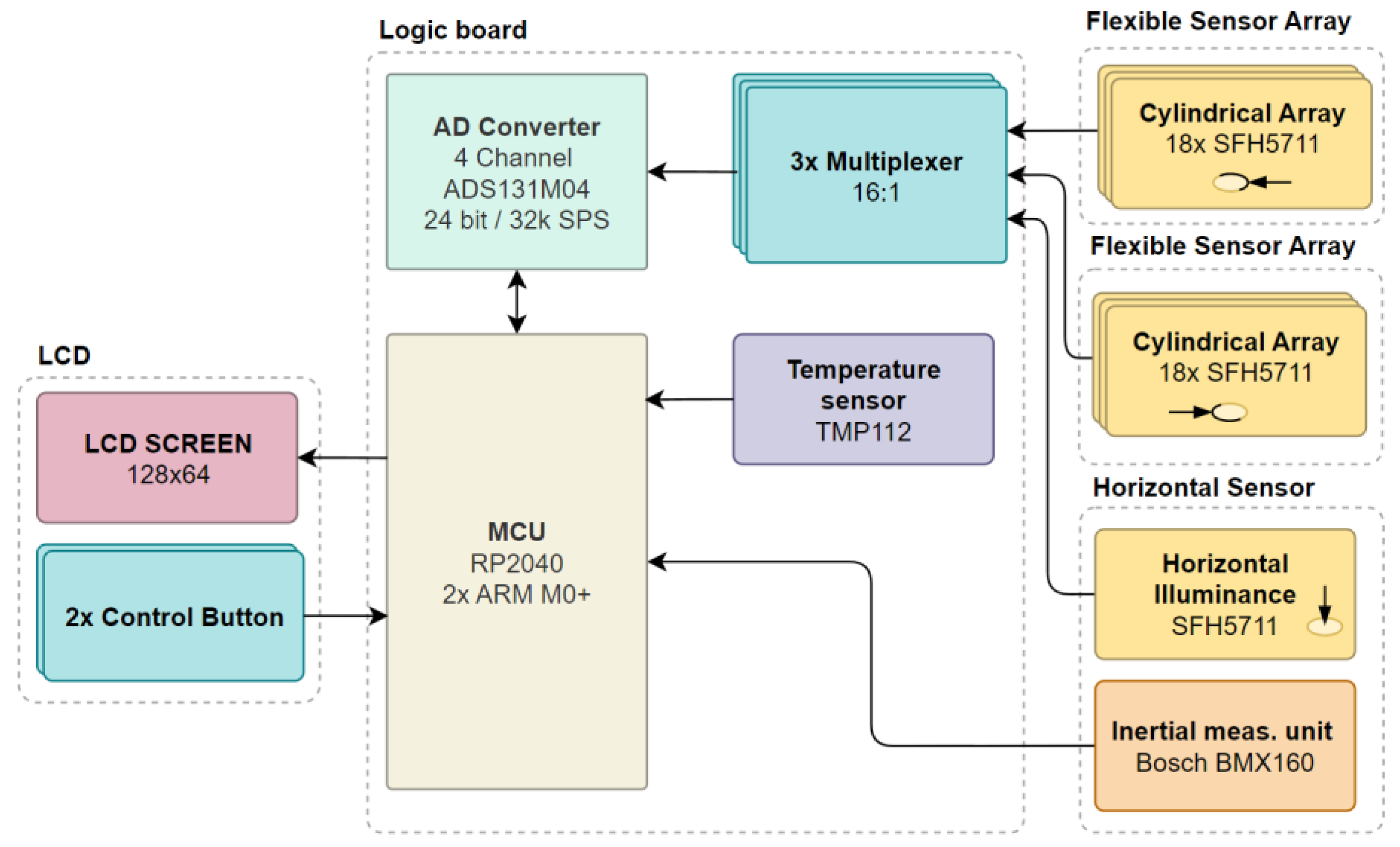
Figure 5.
Signal flow through the multi-sensor system.
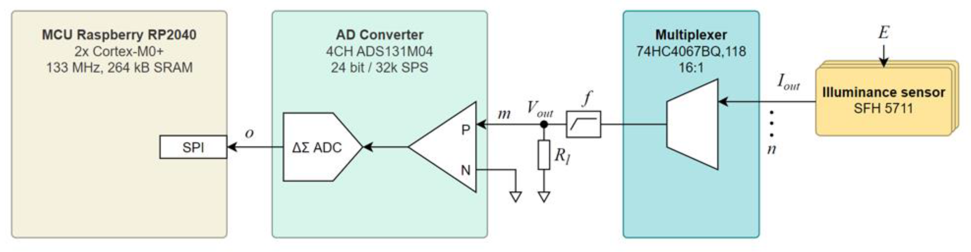
Figure 6.
36 individual vertical illuminances on the cylindrical surface with a step of 10 degrees.
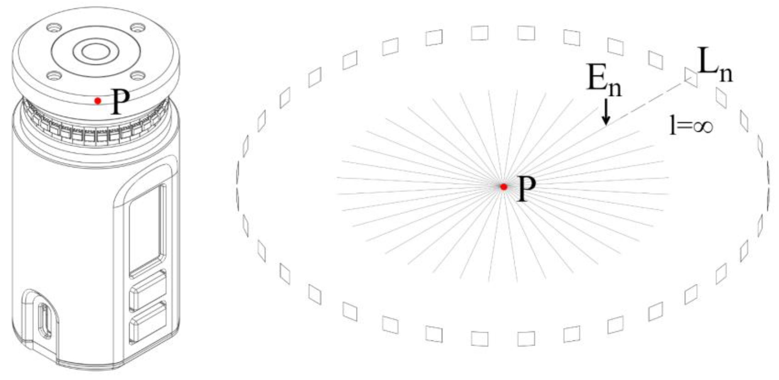
Figure 7.
Polar chart of 36 single illuminance values measured by cylindrical multi-sensor device.
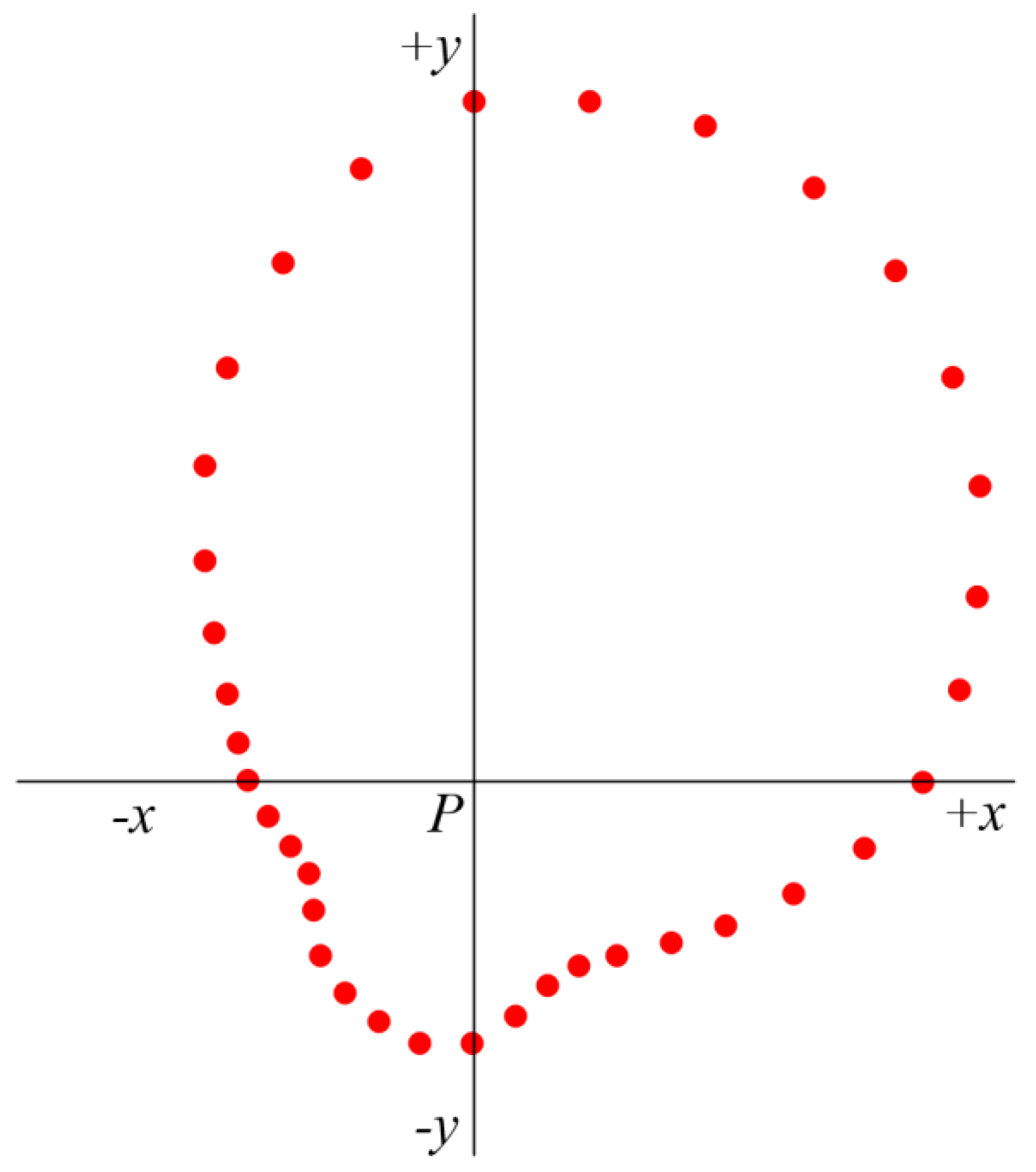
Figure 8.
Two-dimensional illumination solid formed from 36 measured illuminance values.
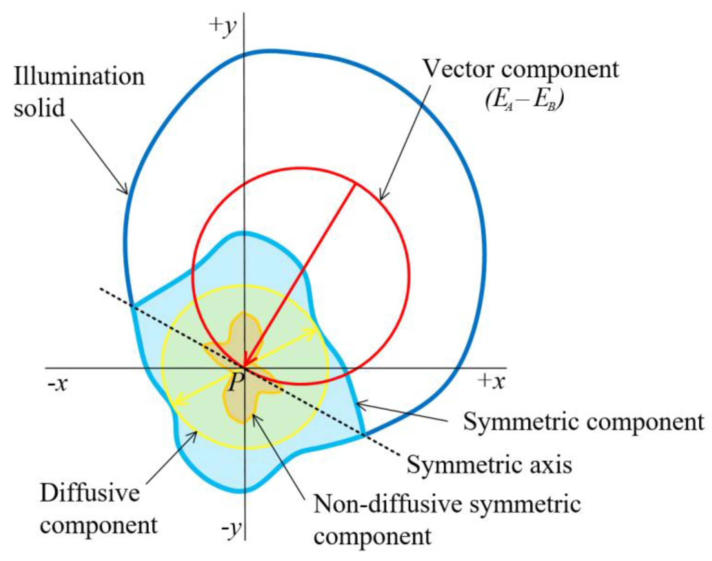
Figure 9.
Simulations of outputs from a multi-sensor located at point P in an environment with a) single point light source, b) two opposite point light sources, and c) three evenly spaced point light sources.
Figure 9.
Simulations of outputs from a multi-sensor located at point P in an environment with a) single point light source, b) two opposite point light sources, and c) three evenly spaced point light sources.
Disclaimer/Publisher’s Note: The statements, opinions and data contained in all publications are solely those of the individual author(s) and contributor(s) and not of MDPI and/or the editor(s). MDPI and/or the editor(s) disclaim responsibility for any injury to people or property resulting from any ideas, methods, instructions or products referred to in the content. |
© 2026 by the authors. Licensee MDPI, Basel, Switzerland. This article is an open access article distributed under the terms and conditions of the Creative Commons Attribution (CC BY) license (http://creativecommons.org/licenses/by/4.0/).
Copyright: This open access article is published under a Creative Commons CC BY 4.0 license, which permit the free download, distribution, and reuse, provided that the author and preprint are cited in any reuse.


