
Submitted:
18 February 2026
Posted:
19 February 2026
You are already at the latest version
Abstract
Gaze analysis often relies on hypothesized, subjectively defined ROIs or heatmaps: ROIs enable condition comparisons but reduce objectivity and exploration, while heatmaps avoid this, they require many pixel-wise comparisons, making differences hard to detect. Here, we propose an advanced data driven approach for analysing gaze behaviour. We use DNNs to classify conditions from gaze patterns, paired with reverse correlation to show where and how gaze differs between conditions. We test our approach on data from an experiment investigating the effects of object specific sound (e.g. church bell ringing) on gaze allocation. ROI-based analysis shows a significant difference between conditions (congruent sound, no sound, phase scrambled sound and pink noise) with more gaze allocation on sound associated objects in the congruent sound condition, however, as expected significance depends on the definition of the ROIs. Heatmaps show some not very clear qualitative differences, but none are significant after correcting for pixelwise comparisons. Our approach shows that sound alters gaze allocation in some scenes, revealing task-specific, non-trivial strategies: fixations are not always drawn to the sound source but shift away from salient features, sometime falling between salient features and the sound source. Overall, the method is objective, data-driven, and enables clear condition comparisons.
Keywords:
saliency
1. Introduction
Perception is inherently active. Within the visual system, high-resolution vision is limited to the fovea. As such, we move our eyes to bring relevant parts of a scene into focus, selecting them for further processing [1,2]. Saliency refers to the potential of visual stimulation to attract gaze. Early research suggested that saliency is primarily driven by bottom-up image properties such as intensity, contrast, motion and Gestalt properties; computed in a pre-attentive manner and independent of the task at hand [2,3,4]. However, the seminal study by Yarbus demonstrated that gaze behaviour can be influenced by cognitive tasks [5]. Later research has broadened the range of higher-level, top-down factors affecting saliency. For instance, it was shown that task demands and value strongly influence gaze [6,7,8]. Additionally, that the visual system directs gaze to task-relevant features – for example, to colour- or motion-diagnostic regions [9,10,11] in a dynamic manner [12]. Furthermore, saliency is suggested to depend on different features at different timepoints, with later, higher latency saccades driven by the task, whilst initial, low-latency features being independent of the task [13].
There are different approaches to investigate gaze behaviour. In previous work, eye movement parameters, such as fixation duration or saccadic amplitude were compared to investigate differences between conditions [14]. However, the spatial information about gaze is typically lost in such approaches or at the very least, limited. For instance, [13] created stimuli, dissociating perceptually relevant information in space, to differentiate between bottom-up and task-driven saliency. Moreover, [15] showed that horizontal or vertical spread in fixations was higher when participants performed width or hight judgments of virtual objects respectively. Analysis of coverage with fixations as utilised in [16], can additionally inform us of how distributed our gaze allocation is and whether it is a result of multi-modal object comparisons or uni-modal comparisons. To be able to do such comparisons, it is necessary to use simplified stimuli, created in a hypothesis driven way. However, it is often interesting to investigate gaze on natural images as they can reveal patterns of visual attention that are more ecologically valid and closer to real-world perception.
Classically, analysis of eye-movements on natural images has focused on comparing gaze parameters (e.g. fixation number) on predefined regions of interest (ROIs), otherwise known as areas of interest. For instance, [17] used ROI analysis to demonstrate that the saliency of social elements in natural images (e.g., presence of people, specifically heads and eyes) was increased when participants were instructed to detect people as fast as possible. The study placed social features amongst other highly salient features which may direct attention away from the task goal. However, this approach has been recently criticised for its multiple limitations [18]. (1) When using natural images, it is not always clear which fixations belong to which object, given insufficient distances between objects or even overlap. (2) The definition of ROI margins is usually subjective, and indeed has the potential to affect the results, as systematically assessed by [19]. (3) To obtain a detailed analysis of gaze allocation such analyses involve comparison of multiple ROIs, inflating the rate of false positives if not corrected [18,20]. For instance [21] ran 105 comparisons between ROIs to investigate allocation of attention on food labels. (4) Another limitation of this approach is that it requires specific hypotheses about how eye movements are used in a specific task and will not reveal other strategies. For instance, fixations landing outside hypothesized ROIs are usually discarded as irrelevant. However, they might instead reflect a sophisticated strategy to simultaneously inspect several locations on the image, by minimising their distance to the fovea and hence achieving the highest possible acuity for multiple locations [22].
Spatial fixation density distributions provide a data-driven way to identify the most salient areas of an image. ROIs can be defined using simple thresholding, selecting regions above a certain fixation frequency [23], or through clustering methods, which group nearby fixations without relying on arbitrary cutoff values [24,25]. While these approaches reliably highlight salient regions, they do not ensure that the resulting ROIs are diagnostic for distinguishing experimental conditions. Therefore, they do not solve the problem of arbitrary ROI selection.
Here, we propose a new data driven approach for analysing differences between conditions in fixation distributions on natural images. The approach involves training a supervised deep neural network (DNNs) to classify the task from fixation distributions. Above-chance classification performance indicates that there are systematic differences between conditions. We then use a classification images approach [26,27,28] to graphically visualise the differences in gaze allocation unique to a specific condition pair comparison. The DNN is trained to classify conditions based on fixation distributions, with random fixations drawn from either condition. These fixation distributions are then classified by the network as belonging to one of the experimental conditions. Averaging across all fixation distributions classified as a particular task reveals the classification image for that task. Differences between the conditions’ classification images allow us to visualise spatial differences in salient elements that are diagnostic of each condition (Figure 2D).
We test this approach on fixation data from an eye-tracking experiment in which participants viewed natural images, each containing a sound emitting object (e.g. church bell). We investigated if a simultaneously played sound consistent with the sound emitting object in the image would affect gaze allocation (i.e. attracting it towards this object), as compared to a no sound condition. There is a body of literature on saliency in the different senses (e.g. [2,29,30]. Effects of multisensory interactions were shown on appearance (e.g. the percept of an ambiguous image was shifted to the object congruent with the simultaneously played sound [31]); precision (e.g. the size of an object can be estimated more precisely when integrating estimates from vision and touch [32]) and search facilitation (e.g. multisensory cues improve visual target detection [33]). However, less is known about how information presented to other senses affect gaze allocation (but [16]).
The new method provided consistent results with traditional ROI analysis and heatmap inspection. However, it is purely data driven and allows for comparing between conditions. Furthermore, as it is not hypothesis-driven, it may provide richer insights in the differences in fixation strategies between the different conditions.
2. Materials and Methods
2.1. Design
The experiment employed a repeated measures design comprising two independent variables sound (congruent vs no sound) and image (10 images), resulting in 20 conditions
2.2. Participants
The final sample consisted of 7 Bournemouth University undergraduate students (5 females, aged between 18 and 22 years (M = 21.60, SD= 0.49) recruited through the SONA platform. Initially, 15 participants were recruited, however, 8 participants were excluded from analysis due to incomplete data, resulting from study disruptions or repeated difficulties in eye-tracking calibration. All participants were naïve to the specific aim of the study and had normal or corrected-to-normal vision and hearing.
As we wanted to compare our novel DNN-based approach with a classic ROI-based factorial design, the sample size was determined using a G*power analysis [34]. The required sample size for a repeated measures ANOVA with one group and four measurements, a significance level of α = .05, a desired power of .8, and a large effect size (η² = .14) is 6 participants. More participants were recruited to ensure sufficient successful experiment completions. The choice of large effect sizes is justified by our previous study on visual saliency, which showed a large effect of task on eye movement allocation [13]. Participants provided informed consent and were compensated for their time with course credits at the rate of 1 credit per hour. The study was approved by the ethics committee of Bournemouth University and conducted in accordance with the 2013 Declaration of Helsinki.
2.3. Stimuli
Ten sound stimuli were selected from publicly available databases [35,36]: church bells chiming, bird tweeting, rocking chair creaking, applause, coins clinking, cicada chirping, helicopter blades beating, bell ringing, heels clacking, waves crashing against the shore. Sounds were cut to two seconds (consistent with the duration of the presentation of the images), containing the most subjectively recognisable part for the target object. For each sound a phase scrambled version was created, to test if potential effects on gaze can be explained by low-level features of the sound, such as frequency composition. Sound volume was adjusted for each participant so that they could clearly hear and recognise the sounds. It remained constant across the experiment. For each sound, consistent colour images were generated with GenCraft, https://gencraft.com/, an AI based software (Figure 1). To be able to investigate the effect of sound on gaze allocation, we tried to exclude that the sound emitting object was fixated because of the salience of its position [37] or its low- or high-level features [2,38] by presenting it alongside other highly salient image features. For example, for the sound of church bells chiming, a scene was designed in which a woman (high-level salient) was presented centrally (salient location) at a picknick (low-level salient), while the church being the target object was presented in the background. Images were presented for 2s in the middle of the screen at a resolution of on grey background (rgb=.5,.5,.5).
2.4. Setup and Eye-Tracking Recording
Participants sat comfortably at a table in front of a monitor (1920 × 1080) in a dark room. Head position was controlled via a chinrest. The viewing distance was 58 cm. We used a desktop-mounted eye-tracker (EyeLink 1000; SR Research Ltd, Osgoode, Ontario, Canada), to record gaze position signals sampled at 1000 Hz. The display was viewed binocularly, but only the right eye was tracked. We performed a standard calibration procedure at the beginning of each experiment [39]. Images were presented on a 24-inch BenQ XL monitor with a resolution of 1920 x 1080 pixels. They were presented in their original sizes in the centre of the screen. We used a standard procedure to colour-calibrate the monitor [40,41], to linearise the screen and make sure that we displayed the desired colour. We measured the gamma curves of each channel and their chromaticity with the Spyder 4 colourimeter (Datacolor, Lawrenceville, NJ). Our screen had the following chromaticity: red primary CIE xyY coordinate (x: 0.6413, y: 0.3274, Y: 57.61 cd/m2), green (x: 0.3104, y: 0.6256, Y: 256.98 cd/m2), and blue (x: 0.1514, y: 0.0568, Y: 26.2 cd/m2). The gamma exponents were 1.913, 1.567 and 2.096, for the red, green and blue channels, respectively.
2.5. Procedure
Before each trial participants were asked to fixate on one of two fixation points (left or right outside of the part of the screen on which the image was presented), to ensure that the first fixation was informative and not biased by the fixation point between the trials [42]. Once fixated, participants pressed the space bar to initiate the trial. Calibration was checked and drift-correction or re-calibration were performed when necessary. In each trial participants viewed for 2s one of ten images, which was either accompanied by a sound or not, depending on the condition. Every, tenth image was displayed on a green background, indicating to participants to decide if this image was “old” (i.e. presented among the previous 9) or “new” (right or left arrow respectively). The order of images and conditions was randomized for each participant. Each image in each condition was presented 5 times.
2.6. Analysis
2.6.1. ROI Analysis
A 10 (image) x 2 (consistent, no sound) repeated-measures ANOVA was used to test for differences in frequency of fixations in the ROIs. We manually defined the ROIs as ellipses around the object. We did not simply segment the objects and used their surface as ROI because due to inaccuracies in both eye-tracking and the human visual system, fixations frequently land outside the target object [18].
To evaluate how robust the results are to small variations in the ROI definition, we created both a smaller and a slightly larger version of each ROI. The smaller ROI was obtained by eroding the original elliptical mask using MATLAB’s morphological operations. Specifically, we used the function strel() to create a disk-shaped structuring element with a radius of pixels corresponding to approximately 0.78 dva. This structuring element was then applied to the ROI mask using the function imerode(), which uniformly shrinks the mask boundaries. As a result, the smaller ellipse was approximately 1.6 degrees of visual angle (dva) smaller at each peripheral point compared to the original ROI. For each image, we computed the proportion of fixations within the ROI, per participants. This was out independent variable for the ANOVA. We conducted two ANOVAs, one per for the larger and one for the smaller ROIs.
2.6.2. DNN-Based Approach
For each image, we trained a deep neural network (DNN) to classify individual fixations into either the sound or the no-sound condition.
2.6.2.1. Training and Validation Data
To train the DNN, we generated a large number of single-fixation images by randomly sampling real fixations from all participants. Crucially, the training and validation sets were created by sampling fixations from different trials: only the fifth and final repetition for each image condition and participant was used for validation. When the training and validation sets were sampled from the same fixation distribution, network performance was close to 100% for each image, suggesting that the network had simply learned to represent the fixation distribution associated with each condition. Performance was lower—but still very high—when we used two different sets of fixations to create the training and validation sets while allowing fixations from the same trial to appear in both sets. This is presumably because fixations that are close in time also tend to be close in space. Our decision to split the data by trials was therefore intended to avoid overfitting by ensuring that training and validation were performed on genuinely independent datasets. We arbitrarily decided to create 180,000 training images and 60,000 validation images. To generate these, each fixation was marked as a value of 1 in a matrix of zeros corresponding to the image size. The resulting image was then Gaussian-filtered with a sigma corresponding to one dva. This was done to approximate the size of the fovea and to account for the resolution of the eye tracker (we accepted calibrations with no more than 0.5 DVA average error). The images were then resized to 227 × 227 pixels for computational efficiency.
2.6.2.2. DNN
We used AlexNet, a popular and relatively simple DNN architecture for image classification. The only modification to the original architecture was adapting the final layer to output two classes corresponding to the experimental conditions of interest. After piloting, we decided for the following optimization parameters: training was performed using stochastic gradient descent with momentum (SGDM), with a mini-batch size of 32 and a maximum of 8 epochs. The initial learning rate was set to and followed a piecewise schedule, decreasing by a factor of 0.1 every 4 epochs. Momentum was fixed at 0.9 and L2 regularization at . Training data were shuffled at every epoch. Model performance was monitored on a held-out validation set at a frequency of 50 iterations, and training was executed on a GPU within a Linux workstation running Ubuntu 22.04.5 LTS, equipped with an AMD Ryzen Threadripper PRO 5955WX CPU (16 cores, 32 threads), 256 GB RAM, and an NVIDIA RTX A6000 GPU with 48 GB VRAM. During training, we applied online data augmentation to the fixation images to improve generalization and reduce overfitting. Augmentations included random rotations (±20°), horizontal and vertical translations (±10 pixels), independent scaling along the x and y axes (0.8–1.2), and random horizontal reflections. These transformations preserve the overall structure of the fixation patterns while introducing variability consistent with natural spatial uncertainty.
2.6.2.3. Statistical Inference
We performed bootstrap inference to evaluate the reliability of our network classification accuracies. To establish empirical chance levels, each network was first trained with randomly shuffled condition labels for each image, yielding accuracies around 50 % (Figure 3A). For networks trained on the true labels, we then resampled 1 000 validation images with replacement and computed classification accuracy on each resampled set, repeating this process 100 times to build an empirical distribution of accuracy estimates. This strategy—sometimes referred to as bootstrapping the test/validation predictions—uses a trained model’s existing predictions on held-out data and resamples them to estimate the sampling distribution of the performance metric without retraining the network on new bootstrap training sets; it is a computationally efficient way to obtain confidence intervals for classifier performance [43]. To account for multiple comparisons across the 10 images, we applied a Bonferroni correction, resulting in a 99.5 % confidence interval. We then assessed whether this interval included the empirical chance level; if it did not, the network’s performance was considered statistically significant.
3. Results
Figure 2A and 2B show heatmaps averaged across participants in the consistent sound and in the no sound conditions, respectively.
3.1. ROIs Analysis
ANOVA on smaller ROIs (Blue ellipse in Fig.2C) shows a significant main effect of sound (F(1,5)=6.708, p=.049, =0.56), main effect of image (F(9,45)= 68.589,p<.001; =0.93) and no significant interaction (F(9,45)=0.884,p=.547; =0.15). This indicates that the proportion of fixations with the ROI is on average high in the consistent sound condition than in the no sound condition, as shown in Figure 3.
With this analysis, the main effect of image is expected because of the different size of the ROIs for different images. In fact, we included as a blocking factor to account for ROI size differences across images. Crucially, when we repeated the ANOVA with the larger ROIs, the main effect of condition was no longer significant (F(1,5)=4.195, p=.096, =0.456). This shows how a little difference in the choice of the ROIs may affect the results.
3.2. DNN-Based Analysis
We tested whether individual fixations could predict experimental condition for each of 10 images. Classification was performed using a separate neural network per image, and accuracy was evaluated on a held-out validation set (see methods section).
Figure 4 shows the validation set accuracy alongside bootstrapped distributions for each image. Bootstrapped 99.5% confidence intervals (Bonferroni-corrected; corresponding to the 0.0025 and 0.9975 quantiles) provided an estimate of variability in classification accuracy.
Across images, classification accuracy exceeded chance levels for 5 out of 10 images. For the five images showing significant classification above chance (images 1, 4, 5, 8, and 9), the lower bound of the bootstrap confidence interval exceeded the empirical chance level, indicating that the observed performance was unlikely to occur by chance (see Table 1). For the remaining images, the bootstrap intervals overlapped with chance, suggesting that classification was not reliable for these stimuli.
3.3. Classification Images
Figure 3D shows the heatmaps revealed by classification image analysis. These heatmaps visualise the spatial differences in condition-diagnostic fixations between the sound and no-sound conditions. While in some cases diagnostic fixations increased at locations corresponding to the expected ROI around the sound-emitting object, in several images the maps reveal more distributed patterns: fixations in the sound condition were reduced on central or otherwise highly salient regions, such as faces, and increased on peripheral or task-relevant areas closer to the sound source. For example, in Image 1, participants fixated less on the central face and more on lateral image regions, whereas in Image 9, gaze shifted away from the face toward the body and the sound-emitting shoe. Overall, these visualisations highlight both expected and distributed condition-diagnostic fixation differences that were not consistently captured by traditional ROI analyses.
4. Discussion
In this study, participants viewed natural images containing a potential sound-emitting object while listening either to a congruent sound or to no sound. Crucially, the sound-emitting objects were intentionally chosen to be not visually salient and were generally not located at the centre of the scene, to avoid simple saliency effects dominating gaze behaviour. We analysed gaze allocation using (1) a classical ROI analysis centred on hypothesised task-relevant regions and (2) a data-driven method that trained a supervised deep neural network (DNN) to classify task condition from single fixations.
Both methods provided evidence that auditory context modulates gaze behaviour. The ROI analysis showed significant main effect sound when fixations fell within predefined spatial regions around the sound-emitting object. However, these effects were highly sensitive to arbitrary ROI definitions: small adjustments to ROI size were sufficient to eliminate statistical significance. In contrast, the DNN classifier reliably decoded condition from single fixations for several images, demonstrating that systematic differences existed in spatial gaze patterns that were not robustly captured within hand-drawn ROIs. Reverse correlation allows us to visualise the spatial locations that drive these classification decisions.
The limitations of ROI-based analysis in eye-tracking research have been a subject of methodological concern in the field. Orquin and Holmqvist [18] describe critical threats to validity in eyetracking research, including flexibility in ROI definition and analysis choices that inflate researcher degrees of freedom and affect interpretability of results. Our analyses empirically demonstrate this concern: slight changes in ROI margin can flip significance for condition effects, a dependency that undermines the reliability of ROI-based inference.
Several studies have developed data-driven ROI generation techniques. For example, applying a threshold to fixation density maps [23] or fixation clustering approaches (e.g., [24,25]) define regions of high fixation density without a priori hypotheses about location. While these algorithms produce objective ROIs based on the data, they remain descriptive: they identify where observers look most frequently, but do not directly test whether fixations in these regions differ between experimental conditions. For instance, in image nine fixations on the shoes are limited and unlikely to define a ROI.
In contrast, our approach uses a discriminative model to test whether fixation distributions as a whole contain condition-relevant information, operationalised as classifier accuracy. This is conceptually analogous to classification image techniques used in vision science (e.g., [44,45,46]) and to probe DNN properties [30,47], where the goal is to identify features predictive of behavioural decisions or DNN responses.
A key advantage of the classification framework over pixel-wise or cluster-wise comparisons is its parsimony. Traditional voxel- or pixel-wise analyses treat each spatial unit as a separate statistical test, leading to thousands of simultaneous comparisons. Controlling false positives in this setting requires strong multiple-comparison corrections or non-parametric cluster-based solutions(e.g. [48]), which rely on spatial smoothing, resampling, and relatively large samples to achieve stable inference. While these approaches are well suited to detecting spatially consistent effects at the group level, they can lose sensitivity when gaze data are sparse, heterogeneous across participants, or weakly aligned in space. In contrast, our decoding-based approach avoids mass-univariate testing altogether by assessing condition information at the level of single fixations. This makes it applicable to data from a single participant or a small number of aggregated participants and robust to spatially distributed effects. By training a single classifier per image to predict conditions from individual distributions, we reduce the inferential problem to a single statistical test per image. Reverse correlation then visualises condition-diagnostic spatial patterns without additional inferential testing at every location, sidestepping the need for explicit multiple comparison corrections and facilitating clear interpretation of spatial differences.
Other machine learning–based approaches have used resampling or classification logic to test hypotheses about gaze behaviour. For example, earlier work used linear classification on eye movement features to assess task effects in scan paths (e.g., [14]). Bootstrap and resampling analyses have been used to assess task dependent fixation differences (e.g., [12,13]). These frameworks share with our method the idea of using data driven inference to evaluate task effects but depend on predefined feature extraction as input to the machine learning model. In contrast, our approach does not require manually defined features; instead, it uses a deep network to learn discriminative spatial patterns from fixation data.
Beyond methodological contributions, our data reveal important behavioural phenomena. One consistent observation was that the presence of sound induced disengagement from faces and central regions of the image—areas that are otherwise highly salient in scene perception. This aligns with substantial literature showing a default bias for central fixation and faces in free viewing [37,49], but importantly shows that auditory context can systematically alter this bias.
For instance, in Image 1, the ROI analysis failed to detect condition differences, but the classifier and associated reverse-correlation maps revealed that participants in the sound condition fixated less on the face and central image area, and more on lateral regions. Similarly, we found that participants’ first fixations were biased toward the image border closest to the starting position of the fixation cross, which was always randomly placed on the left or right of the image. This is consistent with previous research showing start-position effects on early fixations [50,51]. For image 1, the bias appeared stronger when the sound was present, likely because the auditory cue reduced the salience of the centrally located face and facilitated disengagement from it. This suggests an exploratory gaze strategy in the presence of congruent sound, potentially aimed at locating the auditory source through spatial sampling rather than relying on default salient features. In Image 9, fixation differences emerged not only at the sound-emitting shoe but also in a systematic shift of gaze away from the face toward the body, indicating gaze strategies that simultaneously monitor multiple task-relevant regions such as the sound source and the figure producing it. These distributed strategies are consistent with ideas that gaze deployment optimises perceptual efficiency by balancing sampling across locations relevant to the task [22].
Our findings extend the growing evidence that gaze behaviour is shaped by an interaction of bottom-up saliency and top-down task demands. Early models of visual saliency emphasised image features such as intensity and contrast as determinants of fixation locations. However, subsequent work has shown that cognitive instructions and task demands strongly modulate gaze allocation (e.g., task effects in scene viewing, [6,52,53]). Multisensory influences on gaze distribution observed here suggest that saliency in one modality (auditory) can reshape visual saliency landscapes in a way that is distributed and not confined to local object features, consistent with our recent work on cross-modal effects on visual saliency [16].
Although the present classification approach captures robust spatial differences between conditions, future work could extend this framework to investigate temporal dynamics of gaze allocation and interactions with low-level image features. Additionally, integrating classifier outcomes with behavioural performance or neural measures could yield richer models of multisensory attention.
The current results demonstrate that a data-driven classification approach provides a reliable, objective, and interpretable alternative to traditional ROI analyses and clustering methods. By focusing directly on condition-diagnostic regions rather than merely on regions that attract a high number of fixations, this method both avoids subjective parameter choices and reveals spatial gaze effects that would otherwise remain undetected. In doing so, it contributes both a methodological advance and new insights into how multisensory information influences gaze behaviour.
Author Contributions
Conceptualization, M.T. and A.M.; methodology, M.T., A.M., and J.P.; software, M.T., A.M., and J.P.; validation, M.T., A.M., and J.P.; formal analysis, M.T., A.M., and J.P.; investigation, M.T., A.M., and J.P.; resources, M.T., A.M., and J.P.; data curation, M.T., A.M., and J.P.; writing—original draft preparation, M.T., A.M., and J.P.; writing—review and editing, M.T., A.M., and J.P.; visualization, M.T., A.M., and J.P.; supervision, M.T. and A.M.; project administration, M.T. and A.M.; funding acquisition, M.T. All authors have read and agreed to the published version of the manuscript.
Funding
This work was supported by the British Academy (grant number SRG2324\240833).
Institutional Review Board Statement
The study was conducted in accordance with the Declaration of Helsinki and approved by the Institutional Review Board (Ethics Committee) of Bournemouth University (protocol code 52203, date of approval 13/09/2023).
Informed Consent Statement
Informed consent was obtained from all subjects involved in the study. Written informed consent has been obtained from the participants to publish this paper.
Data Availability Statement
Data and MATLAB code are available on github: https://github.com/matteo-toscani-24-01-1985/A-data-driven-approach-for-comparing-gaze-allocation-across-conditions.git.
Acknowledgments
We gratefully acknowledge Serena Sullivan for her invaluable contributions to this work, including the initial conception of the experimental ROI-based factorial design, the creation of the stimuli, and the collection of data during her dissertation research. The image stimuli were generated with AI, GenCraft, https://gencraft.com/.
Conflicts of Interest
The authors declare no conflicts of interest. The funders had no role in the design of the study; in the collection, analyses, or interpretation of data; in the writing of the manuscript; or in the decision to publish the results.
References
- Treue, S. Visual attention: the where, what, how and why of saliency. Current Opinion in Neurobiology 2003, 13, 428–432. [Google Scholar] [CrossRef]
- Itti, L; Koch, C. Computational modelling of visual attention. Nature reviews neuroscience 2001, 2, 194–203. [Google Scholar] [CrossRef]
- Gide, MS; Karam, LJ. A Locally Weighted Fixation Density-Based Metric for Assessing the Quality of Visual Saliency Predictions. IEEE Trans on Image Process 2016, 25, 3852–3861. [Google Scholar] [CrossRef]
- Tatler, BW; Baddeley, RJ; Gilchrist, ID. Visual correlates of fixation selection: Effects of scale and time. Vision research 2005, 45, 643–659. [Google Scholar] [CrossRef]
- Yarbus, AL. Eye Movements During Perception of Complex Objects. In Eye Movements and Vision [Internet]; Springer US: Boston, MA, 1967; pp. 171–211. Available online: http://link.springer.com/10.1007/978-1-4899-5379-7_8.
- Hayhoe, M; Ballard, D. Eye movements in natural behavior. Trends in Cognitive Sciences 2005, 9, 188–194. [Google Scholar] [CrossRef] [PubMed]
- Land, MF. Vision, eye movements, and natural behavior. Vis Neurosci 2009, 26, 51–62. [Google Scholar] [CrossRef]
- Schütz, AC; Braun, DI; Gegenfurtner, KR. Eye movements and perception: A selective review. Journal of vision 2011, 11, 9–9. [Google Scholar] [CrossRef]
- Toscani, M; Zdravković, S; Gegenfurtner, KR. Lightness perception for surfaces moving through different illumination levels. Journal of vision 2016, 16, 21–21. [Google Scholar] [CrossRef]
- Toscani, M; Valsecchi, M; Gegenfurtner, KR. Optimal sampling of visual information for lightness judgments. Proc Natl Acad Sci USA 2013, 110, 11163–11168. [Google Scholar] [CrossRef]
- Toscani, M; Valsecchi, M; Gegenfurtner, KR. Selection of visual information for lightness judgements by eye movements. Philosophical Transactions of the Royal Society B: Biological Sciences 2013, 368, 20130056. [Google Scholar] [CrossRef]
- Toscani, M; Yücel, EI; Doerschner, K. Gloss and speed judgments yield different fine tuning of saccadic sampling in dynamic scenes. i-Perception 2019, 10, 2041669519889070. [Google Scholar] [CrossRef]
- Metzger, A; Ennis, RJ; Doerschner, K; Toscani, M. Perceptual task drives later fixations and long latency saccades, while early fixations and short latency saccades are more automatic. Perception 2024, 53, 501–511. [Google Scholar] [CrossRef]
- Greene, MR; Liu, T; Wolfe, JM. Reconsidering Yarbus: A failure to predict observers’ task from eye movement patterns. Vision research 2012, 62, 1–8. [Google Scholar] [CrossRef]
- Aizenman, AM; Gegenfurtner, KR; Goettker, A. Oculomotor routines for perceptual judgments. Journal of Vision 2024, 24, 3. [Google Scholar] [CrossRef]
- Toscani, M; Gather, M; Seiss, E; Metzger, A. EXPRESS: Effect of prior haptic object exploration on eye-movements. Quarterly Journal of Experimental Psychology 2026, 17470218261417305. [Google Scholar] [CrossRef]
- End, A; Gamer, M. Task instructions can accelerate the early preference for social features in naturalistic scenes. R Soc open sci 2019, 6, 180596. [Google Scholar] [CrossRef]
- Orquin, JL; Holmqvist, K. Threats to the validity of eye-movement research in psychology. Behav Res. 2018, 50, 1645–1656. [Google Scholar] [CrossRef]
- Orquin, JL; Ashby, NJS; Clarke, ADF. Areas of Interest as a Signal Detection Problem in Behavioral Eye-Tracking Research. Behavioral Decision Making 2016, 29, 103–115. [Google Scholar] [CrossRef]
- Von Der Malsburg, T; Angele, B. False positives and other statistical errors in standard analyses of eye movements in reading. Journal of Memory and Language 2017, 94, 119–133. [Google Scholar] [CrossRef]
- Antúnez, L; Vidal, L; Sapolinski, A; Giménez, A; Maiche, A; Ares, G. How do design features influence consumer attention when looking for nutritional information on food labels? Results from an eye-tracking study on pan bread labels. International Journal of Food Sciences and Nutrition 2013, 64, 515–527. [Google Scholar] [CrossRef]
- Hitzel, E; Tong, M; Schütz, A; Hayhoe, M. Objects in the peripheral visual field influence gaze location in natural vision. Journal of Vision 2015, 15, 783. [Google Scholar] [CrossRef]
- Wooding, DS. Fixation maps: quantifying eye-movement traces 2002, 31–36.
- Privitera, C; Azzariti, M; Stark, L. Locating regions-of-interest for the Mars Rover expedition. International Journal of Remote Sensing 2000, 21, 3327–3347. [Google Scholar] [CrossRef]
- Santella, A; DeCarlo, D. Robust clustering of eye movement recordings for quantification of visual interest; 2004; pp. 27–34. [Google Scholar]
- Ahumada, A; Lovell, J. Stimulus Features in Signal Detection. The Journal of the Acoustical Society of America 1971, 49, 1751–1756. [Google Scholar] [CrossRef]
- Beard, BL; Ahumada; Jr., AJ. Technique to extract relevant image features for visual tasks; Rogowitz, BE, Pappas, TN, Eds.; San Jose, CA, 1998; pp. 79–85. Available online: http://proceedings.spiedigitallibrary.org/proceeding.aspx?articleid=936723.
- Eckstein, MP; Ahumada, AJ. Classification images: A tool to analyze visual strategies. Journal of Vision 2002, 2, i. [Google Scholar] [CrossRef]
- Kayser, C; Petkov, CI; Lippert, M; Logothetis, NK. Mechanisms for Allocating Auditory Attention: An Auditory Saliency Map. Current Biology 2005, 15, 1943–1947. [Google Scholar] [CrossRef]
- Metzger, A; Toscani, M; Akbarinia, A; Valsecchi, M; Drewing, K. Deep neural network model of haptic saliency. Sci Rep. 2021, 11, 1395. [Google Scholar] [CrossRef]
- Williams, JR; Markov, YA; Tiurina, NA; Störmer, VS. What You See Is What You Hear: Sounds Alter the Contents of Visual Perception. Psychol Sci. 2022, 33, 2109–2122. [Google Scholar] [CrossRef]
- Ernst, MO; Banks, MS. Humans integrate visual and haptic information in a statistically optimal fashion. Nature 2002, 415, 429–433. [Google Scholar] [CrossRef]
- Hancock, PA; Mercado, JE; Merlo, J; Van Erp, JBF. Improving target detection in visual search through the augmenting multi-sensory cues. Ergonomics 2013, 56, 729–738. [Google Scholar] [CrossRef]
- Faul, F; Erdfelder, E; Buchner, A; Lang, AG. Statistical power analyses using G*Power 3.1: Tests for correlation and regression analyses. Behavior Research Methods 2009, 41, 1149–1160. [Google Scholar] [CrossRef]
- Piczak, KJ. ESC: Dataset for Environmental Sound Classification. In Proceedings of the 23rd ACM international conference on Multimedia [Internet]; ACM: Brisbane Australia, 2015 [cited 2025 Oct 15; pp. 1015–1018. Available online: https://dl.acm.org/doi/10.1145/2733373.2806390.
- Public Domain Sounds Backup [Internet]. Available online: https://pdsounds.tuxfamily.org/.
- Tatler, BW. The central fixation bias in scene viewing: Selecting an optimal viewing position independently of motor biases and image feature distributions. Journal of vision 2007, 7, 4–4. [Google Scholar] [CrossRef]
- Einhäuser, W; Spain, M; Perona, P. Objects predict fixations better than early saliency. Journal of vision 2008, 8, 18–18. [Google Scholar] [CrossRef] [PubMed]
- Granzier, JJ; Toscani, M; Gegenfurtner, KR. Role of eye movements in chromatic induction. JOSA A 2012, 29, A353–65. [Google Scholar] [CrossRef]
- Gil Rodríguez, R; Bayer, F; Toscani, M; Guarnera, D; Guarnera, GC; Gegenfurtner, KR. Colour calibration of a head mounted display for colour vision research using virtual reality. SN Computer Science 2022, 3, 1–10. [Google Scholar] [CrossRef]
- Toscani, M; Gil, R; Guarnera, D; Guarnera, G; Kalouaz, A; Gegenfurtner, KR. Assessment of OLED head mounted display for vision research with virtual reality; IEEE, 2019; pp. 738–745. [Google Scholar]
- Arizpe, J; Kravitz, DJ; Yovel, G; Baker, CI. Start Position Strongly Influences Fixation Patterns during Face Processing: Difficulties with Eye Movements as a Measure of Information Use. In PLoS ONE; Barton, JJS, Ed.; 2012; Volume 7. [Google Scholar]
- Raschka, S. Machine learning Q and AI: 30 essential questions and answers on machine learning and AI; No Starch Press, 2024. [Google Scholar]
- Brenner, E; Granzier, JJ; Smeets, JB. Perceiving colour at a glimpse: The relevance of where one fixates. Vision Research 2007, 47, 2557–2568. [Google Scholar] [CrossRef] [PubMed]
- Neri, P; Levi, DM. Receptive versus perceptive fields from the reverse-correlation viewpoint. Vision research 2006, 46, 2465–2474. [Google Scholar] [CrossRef]
- Hansen, T; Gegenfurtner, KR. Classification images for chromatic signal detection. Journal of the Optical Society of America A 2005, 22, 2081–2089. [Google Scholar] [CrossRef] [PubMed]
- Metzger, A; Toscani, M. Unsupervised learning of haptic material properties. Elife 2022, 11, e64876. [Google Scholar] [CrossRef]
- Lao, J; Miellet, S; Pernet, C; Sokhn, N; Caldara, R. I map4: An open source toolbox for the statistical fixation mapping of eye movement data with linear mixed modeling. Behavior research methods 2017, 49, 559–575. [Google Scholar] [CrossRef]
- Cerf, M; Frady, EP; Koch, C. Faces and text attract gaze independent of the task: Experimental data and computer model. Journal of vision 2009, 9, 10–10. [Google Scholar] [CrossRef] [PubMed]
- Rothkegel, LO; Trukenbrod, HA; Schütt, HH; Wichmann, FA; Engbert, R. Influence of initial fixation position in scene viewing. Vision research 2016, 129, 33–49. [Google Scholar] [CrossRef] [PubMed]
- Arizpe, J; Kravitz, DJ; Yovel, G; Baker, CI. Start position strongly influences fixation patterns during face processing: Difficulties with eye movements as a measure of information use. PloS one 2012, 7, e31106. [Google Scholar] [CrossRef] [PubMed]
- Yarbus, AL. Eye movements during fixation on stationary objects. In Eye movements and vision; Springer, 1967; pp. 103–127. [Google Scholar]
- Land, MF. Vision, eye movements, and natural behavior. Visual neuroscience 2009, 26, 51–62. [Google Scholar] [CrossRef]
Figure 1.
Visual Stimuli. Each image depicts an object that produces a sound but is not visually salient. From left to right and top to bottom, the objects are: a belltower, a bird, a rocking chair, clapping hands, tossing coins, crickets, a helicopter, a school bell, high hills, and the sea. These objects are not presented at the centre of the images, where fixations naturally tend to land.

Figure 2.
Heatmaps and regions of interest. (A) Heatmaps for the consistent sound condition averaged across participants, and (B) heatmaps for the no-sound condition averaged across participants; fixation density increases from no colour to blue, yellow, and red. (C) Regions of interest (ROIs), with smaller ROIs indicated by blue ellipses and larger ROIs by red ellipses. (D) Heatmaps revealed by classification image analysis, where blue indicates negative differences (i.e., fewer condition-diagnostic fixations in the consistent sound condition) and red indicates positive differences (i.e., more condition-diagnostic fixations in the consistent sound condition); colour intensity reflects the absolute magnitude of the difference. Images surrounded by a red square are those for which we could significantly classify the condition based on fixations using our DNN-based approach.
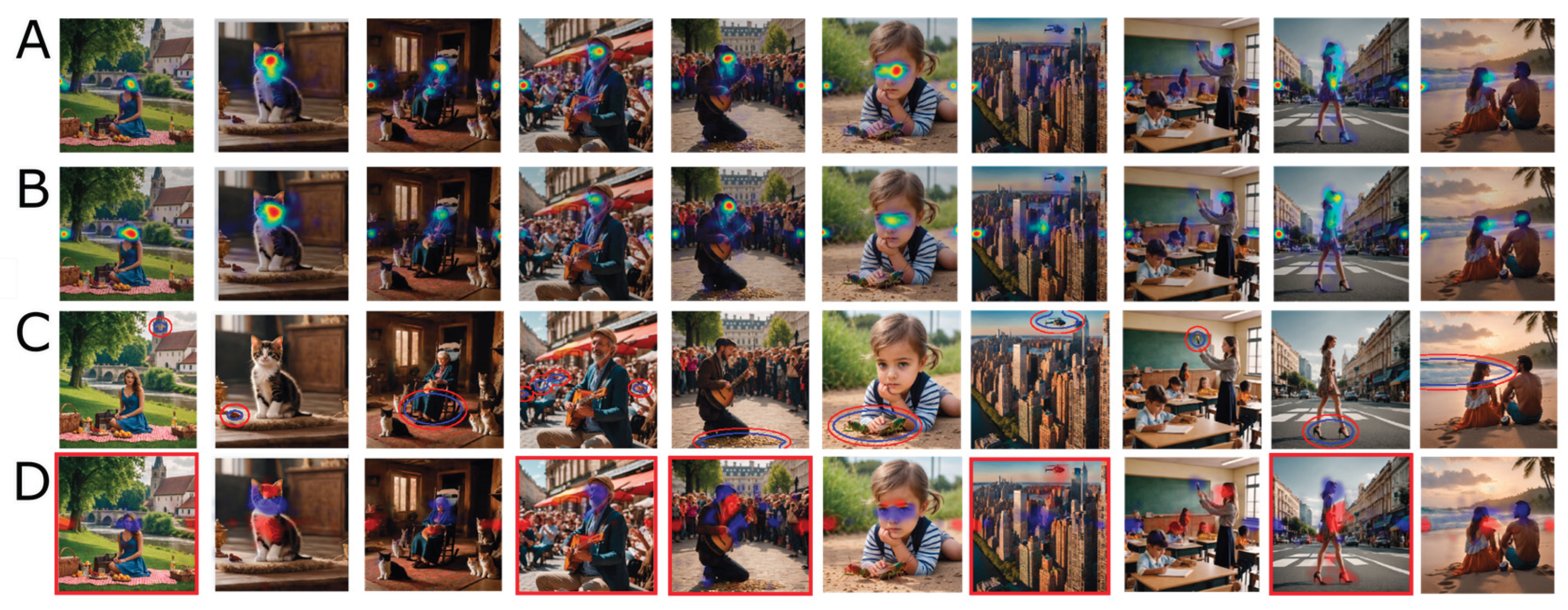
Figure 3.
Proportion of Fixations Within ROI, on the y-axis, averaged across images and across participants. Consistent Sound and No Sound conditions, on the x-axis. Error bars indicate the standard error of the mean across participants.
Figure 3.
Proportion of Fixations Within ROI, on the y-axis, averaged across images and across participants. Consistent Sound and No Sound conditions, on the x-axis. Error bars indicate the standard error of the mean across participants.
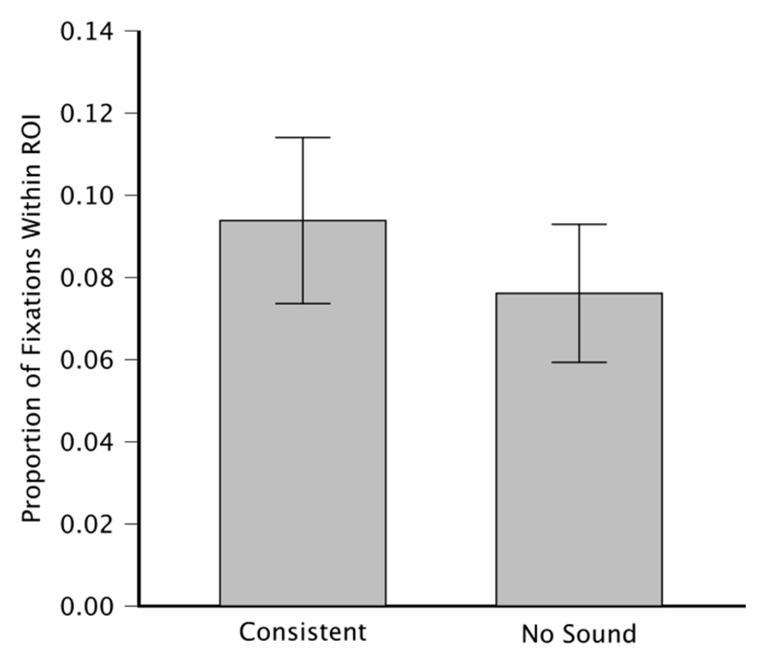
Figure 4.
Classification Results. Image on the x-axis, accuracy on the y-axis, in percentage. Black circles indicate classification accuracy computed on the whole validation set. The violine plot shaded areas (in green) represent the kernel density estimate of the data, indicating the distribution’s shape and relative frequency. The vertical lines represent the interquartile range. Stars indicate the images for which classification was significantly above chance (see Table 1). The horizontal line represents the average empirical chance level, and the shaded (in read) area around it represents its 95% confidence interval.
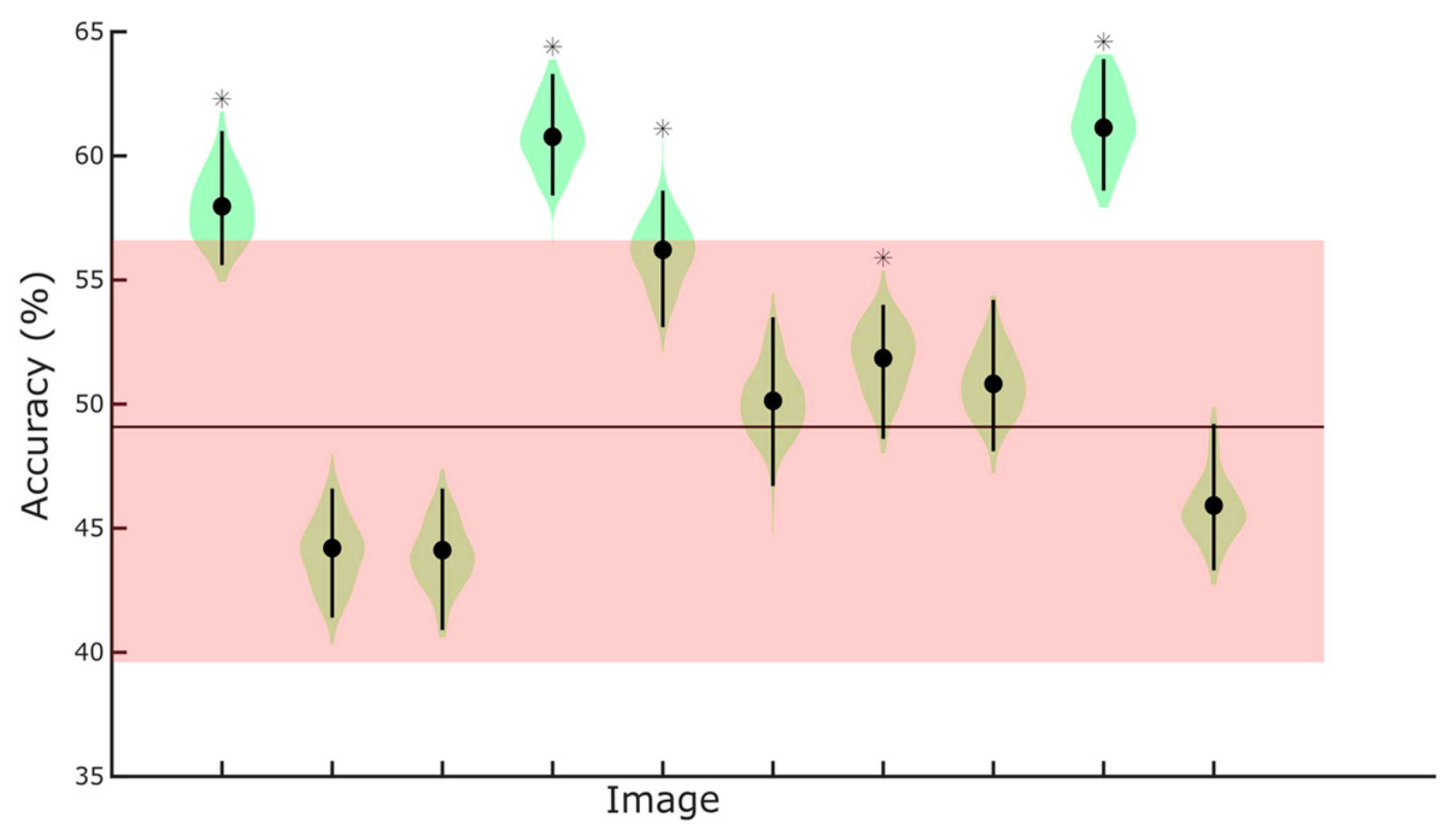

Table 1.
Bootstrap analysis.
| Chance Accuracy | 0.0025 quantile accuracy | 0.9975 quantile accuracy |
|---|---|---|
| 0.4484 | 0.5490 | 0.6180 |
| 0.5042 | 0.4030 | 0.4800 |
| 0.5499 | 0.4060 | 0.4740 |
| 0.4075 | 0.5640 | 0.6390 |
| 0.4903 | 0.5210 | 0.6060 |
| 0.5501 | 0.4480 | 0.5450 |
| 0.4483 | 0.4800 | 0.5540 |
| 0.5215 | 0.4720 | 0.5440 |
| 0.4538 | 0.5790 | 0.6410 |
| 0.5383 | 0.4270 | 0.4990 |
Disclaimer/Publisher’s Note: The statements, opinions and data contained in all publications are solely those of the individual author(s) and contributor(s) and not of MDPI and/or the editor(s). MDPI and/or the editor(s) disclaim responsibility for any injury to people or property resulting from any ideas, methods, instructions or products referred to in the content. |
© 2026 by the authors. Licensee MDPI, Basel, Switzerland. This article is an open access article distributed under the terms and conditions of the Creative Commons Attribution (CC BY) license (http://creativecommons.org/licenses/by/4.0/).
Copyright: This open access article is published under a Creative Commons CC BY 4.0 license, which permit the free download, distribution, and reuse, provided that the author and preprint are cited in any reuse.


