
Submitted:
16 February 2026
Posted:
24 February 2026
You are already at the latest version
Abstract
Accurate monitoring of iron and steel factories is crucial for both economic efficiency and environmental protection. Steel plays a key role in the European (EU) economy, including its green transition, due to its use across numerous strategically important sectors. The EU steelmaking industry is the world’s third largest producer, with sites distributed across more than 20 Member States. Steel plants sustain many regional economies, emphasizing their socio-economic and political significance. Industrial complexes are major heat sources composed of multiple small-scale operating assets, which can be effectively analyzed using heterogenous infrared satellite indicators at medium to high spatial resolution. In this study, for the first time, a multi-source approach integrating two thermal anomaly indices, the Thermal Anomaly Index (TAI) and the Normalized Hotspot Index (NHI), derived from 20m infrared satellite imagery, is proposed. The ArcelorMittal facilities in Asturias, Spain (Avilés and Gijón), operated by the world’s second largest steel producer, were selected to calibrate and validate the methodological framework. Preliminary results show a strong correlation (R2 ≈ 0.7₋1.00) between detected activations (used as proxies for production rates) and ground-truth data (annual crude steel and pig iron production) for 2016˗2024, across multiple spatial scales (from national to individual assets). Application to steelmaking facilities in France and Germany further confirms the robustness of the approach. Independent data on steel production are essential to better assess the environmental impacts of the sector, as production levels are directly linked to emissions and pollution. The satellite-based methodology presented here provides an objective means to quantify steel output where official data are incomplete or unavailable, enabling consistent assessments of national exposure to steelmaking activities and progress toward decarbonization.
Keywords:
iron/steel facilities
; ArcelorMittal Asturias
; Sentinel 2/MSI
; radiance
; reflectance
; TAI
; NHI
; thermal anomaly detection
1. Introduction
The steel industry plays a fundamental role in modern civilization, underpinning daily life and industrial manufacturing worldwide [1,2]. Steel is one of the most important metals for the global economy, providing essential materials for vehicles, machinery, buildings, industrial plants, energy production and more [3]. It also plays a central role in the transition to a greener economy, supporting the development of electric vehicles, wind turbines, solar arrays, and a wide range of clean-technology products. Moreover, steel is crucial for a circular economy, as many of its applications and components can be efficiently recycled, reused and remanufactured [4].
Driven by rapid urbanization and industrialization, the demand for steel has increased over recent decades [2] and is expected to continue growing substantially in the coming years. Planned increases in global steelmaking capacity could reach up to 165 million metric tons between 2025 and 2027 [5] due to its direct relationship to population, gross domestic product growth and overall industrialization [6,7]. Understanding this sector is especially urgent because of its significant role to climate change [1,8]. The dominant steelmaking technology worldwide remains the conventional, highly carbon dioxide (CO2) ₋ intensive blast furnace – basic oxygen furnace (BF˗BOF) route, which relies on iron ore and coke as key inputs [7]. Large volumes of CO2-rich gases are released during various stages of the steelmaking process [7]. As the second largest energy consumer in the global industrial sector, the iron and steel industries are highly dependent on fossil fuels and release massive amounts of CO2 [8,9]. Blast furnaces operating at ~1600 °C consume large quantities of fossil fuels, and conservative estimates indicate that the industry is responsible for about 8% of global greenhouse gas emissions [6]. In 2023, 1.92 tonnes of CO2 were emitted per ton of crude steel produced [3]. Although the CO2 intensity of crude steel production has slightly decreased in recent years, progress remains insufficient to meet the Net Zero Emissions by 2050 Scenario [10]. Decarbonizing the iron and steel industry is therefore essential to achieve global climate mitigation targets [6]. Producers plan to cut emissions by investing in clean power, innovative technologies, and improved process efficiency. At the same time, large steel firms have engaged in automation and digitalization efforts over recent decades, enhancing production efficiency and operational monitoring capabilities [1].
At the global scale, only a few countries in Asia, America and Europe account for roughly 70% of global crude steel production in 2024 (Figure 1).
China (~65%), the United States (~55%) and Germany (~27%) are the leading producers in their respective continents (Figure 1a), while within the EU the steel sector is dominated by Germany, Italy, Spain and France (Figure 1b) [11].
Considering the steelmaking relevance for human life, transparent and reliable data are essential to monitor global steel production and its environmental impact, yet such information remains scarce [9]. Satellite-based monitoring offers a valuable and independent way to track plant operations and detect production changes, complementing official statistics. Recent initiatives like TransitionZero [12]) and Climate TRACE (Tracking Real-Time Atmospheric Carbon Emissions) [13] are improving transparency by integrating AI, remote sensing, and open datasets. Maintaining updated, detailed inventories of industrial facilities is crucial for evaluating mitigation policies, and remote sensing is proving increasingly effective for monitoring steel industry activity [14,15].
This work investigates the applicability of the Thermal Anomaly Index (TAI, [16]) and the Normalized Hotspot Index (NHI, [17,18,19]) for detecting thermal anomalies associated with steel plants in the Asturias region of Spain, where major ArcelorMittal (a multinational steel manufacturing, ranked 2nd as the largest steel producer in the world [20], are located (Gijón and Avilés). The objective is to evaluate the ability of these satellite metrics to provide independent insights into national level steelmaking activity. The steel industry supports economic and societal growth but remains a major source of greenhouse gas emissions, with total emissions rising as production increases unless strong decarbonization measures are adopted [21,22]. The Steel Climate Impact 2025 report shows that total greenhouse gas emissions from the steel sector are largely driven by production volumes, with increases in steel output generally leading to higher absolute emissions despite improvements in emission intensity per ton of steel [23]. [21] show that while technological improvements can substantially reduce greenhouse gas emission intensity per ton of steel, total emissions remain strongly linked to overall steel production volumes and may increase when demand growth outweighs efficiency gains. The availability of satellite-based products, providing independent information on steelmaking activities across space and time domains, represents a valuable resource for policymakers engaged in monitoring and reducing GHG emissions.
2. Literature Review
This section reviews satellite-based approach for monitoring industrial sites. Developing accurate and comprehensive datasets in this sector is challenging due to limited ‘ground truth’ data and the inherent spatial, spectral, and temporal constraints of satellite imagery. Nevertheless, these methods have effectively addressed information gaps and supported the development and parameterization of models for quantifying steelmaking processes [1,2,6,8]. Recent methodological advances reported between 2018 and 2024 are summarized in Table 1.
A review of the studies in Table 1 confirms the feasibility of detecting industrial heat sources from satellite data, with shortwave–mid-infrared fire products particularly effective for capturing steelmaking activity as high-temperature anomalies. Most applications focus on China, with fewer at the global scale.
VIIRS (Visible Infrared Imaging Radiometer Suite) data enabled global and national inventories of industrial hotspots, reaching ~77% accuracy at 750 m [14] and supporting refined heat-flux mapping at 375 m using a multiple-sliding-window method [32]. ASTER thermal observations further improved the detection of hotspots below 700 K with 85.13% accuracy using a threshold-based TAI, and provided Fire Radiative Power (FRP) estimates strongly correlated with simulated values, though sensitive to atmospheric and background conditions [25].
Thermal sharpening of MODIS LST with Landsat-8 TIR [15] enhanced the spatial detail of industrial emissions, yielding strong associations with surface indices (R2 > 0.84), but performance may degrade when the resolution gap between the satellite pixel and the target source scale of interest increases substantially. Additional analyses found solid correlations between industrial activity and VIIRS/Landsat-8 fire products [8,26,27], though links with CO2 and N2O remained weak due to coarse emission datasets.
Landsat-8 at 100 m enabled factory-level thermal mapping of iron and steel plants, with LST contrasts capturing functional areas and operational patterns [24]. Seasonal adjustment of LST [9] further isolated production-related thermal signals.
Sentinel-2-based indices provide the most accurate recent approaches: the TAI achieved 99.84% global hotspot-detection accuracy [16], while the NHI—originally for volcanic anomaly detection—proved effective for industrial sources such as gas flaring and for national-scale radiative-power estimation [28˗31]. Both rely on fixed thresholds, which may affect sensitivity across environments.
Satellite-based assessments remain influenced by sensor characteristics, retrieval algorithms, atmospheric conditions, and the intrinsic heterogeneity of industrial facilities. Nonetheless, the combination of Sentinel-2 Multispectral Imager (MSI) data with TAI and NHI offers an effective trade-off between spatial, spectral, and temporal resolution, motivating their use to investigate steelmaking plants in Asturias (Spain) and subsequently in France and Germany.
3. The Study Cases
Spain plays a significant role in European steel production, though its global share remains limited. In 2024, it was the third-largest EU producer, accounting for ~9% of EU output, behind Germany and Italy, and ahead of France [33]. Globally, Spain represents only 0.7% of total production, in a market dominated by China, which alone produces over half of the world’s steel (Figure 1). Spain ranked 17th in 2023–2024, producing 11.4–11.9 million tons of crude steel—about 90 times less than China [3].
The Spanish steel sector features modern facilities, strong European integration, and growing attention to sustainability. Most output serves construction, automotive, and industrial sectors. Electric arc furnace (EAF) production is increasingly important: in 2024, ~69% of Spanish steel came from EAF, compared to ~31% from the blast furnace–basic oxygen furnace (BF–BOF) route [3].
Spain has 14 operating steel mills: two BF–BOF plants (Gijón and Avilés) and twelve EAF facilities [34]. Gijón and Avilés, located in Asturias near port services, are key to national output, with nominal capacities of 1.2 and 4.2 million tonnes per year, respectively [35]. Between 2021–2024, they emitted on average ~0.6 and ~2.4 tCO2e per ton of steel produced (100-year horizon) [13].
Figure 2 shows the two Spanish plants and their sub-categories responsible for steelmaking (highlighted in white).
This study investigated the subcategories of heat-releasing industrial plants to test and fine-tune selected satellite metrics and thermally characterize each plant. Each feature was analyzed in the space-time domain to assess its behavior within steel factories and to evaluate the role of individual assets in the overall steelmaking process.
4. Data and Methods
4.1. Data
Data used in this work belongs to two categories. Satellite data/products were used for implementing the methods (Section 4.1.1). Ground-truth data about steel/iron production were used to validate the results achieved (Section 4.1.2).
4.1.1. Daytime Satellite Products: the TAI and NHI Indices
Hot sources emit most of their thermal radiation in the InfraRed (IR) region of the electromagnetic spectrum. The peak of thermal emissions shifts from mid-infrared (MIR) region (3–3.5 µm for a hot source at 800–1000 K) to shortwave infrared (SWIR) region at higher temperatures (e.g., 2.2 µm at ∼1400 K, 1.6 µm at ∼1800 K). Electromagnetic radiation from industrial heat sources can be remotely sensed using indices that exploit their elevated radiance at these wavelengths. In this work, the TAI and NHI metrics, based on Near Infrared (NIR) and SWIR infrared bands acquired by MSI on Sentinel 2A and 2B (S2) (tile T29TQJ, time 11:15-11:30 UTC), at 20m spatial resolution, were selected and computed following the procedures in [16] and [17˗19], respectively. Harmonized Collection MSI Level₋1C data were processed to implement TAI and NHIs. The TAI and NHIs codes run in Google Earth Engine, leveraging all images acquired over Gijón and Avilés areas (Figure 2a and Figure 2b, respectively) between 2016 and 2024.
The TAI index is a tri-spectral index based on reflectance data [16]:
where ρ2.2, ρ1.6 and ρ0.8 refer to reflectance at 2.2, 1.6 and 0.8μm (B12, B11, B8A). Prior to its calculation, saturated pixels were identified using the tests ρ1.6≥1 and ρ2.2≥1 and removed from further analysis. Saturation of MSI bands 12 and 11 due to high energy and extensive high-temperature anomalies can lead to negative TAI values [16]. Consequently, approximately 5% of pixels in both regions of interest were found to be saturated and were removed.
The NHIs are implemented on radiance format data as bi-spectral indices [17,18,19]:
where L refers to radiance, and 2.2, 1.6 and 0.8 correspond to the SWIR2 (B12), SWIR1 (B11) and NIR (B8A) band center wavelengths, respectively.
The NHISWIR index takes positive values in the presence of low-to-moderate thermal anomalies, when SWIR2 radiance exceeds SWIR1. More intense thermal features often produce a large increase in SWIR1 radiance, which, combined with the lower saturation radiance of SWIR2, can lead to negative NHISWIR values, also observed over background and cloudy areas.
Conversely, NHISWNIR assumes positive values primarily in the presence of intense thermal anomalies (in terms of temperature and size), due to SWIR1 exceeding NIR radiance [17,18,19,28,29].
By combining the two indices, the NHI algorithm can efficiently map high-temperature features (e.g., [19]) with some limitations, including:
- i)
- dependence on clouds and degassing plumes, which may partially or completely obscure hot targets;
- ii)
- potential missed detections for weak thermal activity;
- iii)
- underestimation of thermal anomalies for extremely hot targets, due to pixel saturation in both MSI SWIR bands.
In this work, a total of 1246 MSI observations from 2016 to 2024 comprised the satellite dataset. Unlike NHI, TAI computation requires selecting clear pixels to exclude false alarms caused by clouds or data artifacts, a step optionally recommended by [16]. The average omission error of the MSI cloud mask ranges from ~ 40% to ≥ 87% for images containing opaque clouds with sizeable transitional zones [16,36]. For this reason, the authors preferred tolerating false positives rather than discarding real hotspots misclassified as clouds. Visual inspection of sample satellite observations over the regions of interest confirmed that the risk of misclassification is negligible, nearly zero.
The TAI and NHI metrics detect thermal anomalies related to both natural and anthropogenic phenomena, particularly those with emission peaks in the SWIR bands. Using reflectance and radiance data may provide different information for the same target. Explaining the nature of these differences is beyond the scope of this paper, as the focus is on assessing the ability of these indices to provide reliable information on thermal anomalies occurring at steel/iron plants under daytime conditions. Their positive response may allow them to serve as proxies for quantifying steelmaking activity through independent daytime satellite products.
Applying fixed thresholds (generally greater than 0) to TAI and NHI allows for selecting pixels hosting hotspots [16,17,19,28,29,30,31,37,38], while the temporal occurrence frequency is used to filter out industrial facilities with persistent high-temperature sources (e.g., blast furnaces, rotary kilns, chimneys, gas stacks) (e.g., [16]. [30,31]).
Investigating steelmaking facilities with TAI and NHIs for the first time required a preliminary analysis of their behavior as far as these kinds of hot objects are observed.
In the following, TAI and NHI thresholds were fine-tuned to maximize the indices performance for customized targets, specifically heavy industries. To this aim, B12, B11 and B8A reflectance (for TAI-based analysis) and radiance (for NHI analysis) along spatial transects crossing representative sub-assets within the Gijón and Avilés plants were used to investigate the spectral signature of hot and background pixels. MSI images acquired on 29 January 2022 for Gijón (Figure 3a) and on 17 September 2018 for Avilés (Figure 4a) were used for this test.
SWIR reflectance and radiance signals show a clear increase when crossing hot pixels, for both reflectance and radiance (see the corresponding white and black transects in Figure 3 and Figure 4). Consequently, peaks of TAI and NHI values appear along the profiles, with positive values for TAI and values for NHIs that are less negative or greater than zero. To identify the optimal threshold for each metric capable of selecting thermal anomalies related to steelmaking processes, scatter density plots of hot sub-assets from Gijón and Avilés were collected and analyzed in the feature space of bands 11, 12 and 8A (Figure 5). In Figure 5, Gijón sub-assets are represented by yellow squares, Avilés sub-assets by green triangles, and cloudy pixels by grey dots.
From Figure 5, thresholds of 0.10 for TAI (TAI≥0.1) and -0.5 for NHIs (NHI≥-0.5) were identified as optimal for reliably selecting hot pixels in steelmaking areas while minimizing cloud misclassification. The plots show that pixels from steel plants predominantly lie above these threshold lines, regardless of the plant considered, whereas clouds cluster below them. This supports the effectiveness of these metric thresholds in differentiating hot industrial pixels from cloud contamination. Although hot pixels can sometimes exhibit spectral behavior similar to clouds (see yellow and green point below the black lines), the chosen thresholds provide a quite clear separation between these two classes. Applying this selection filter, thermal anomalies within each steel plant, referred as “activations” (i.e., thermally anomalous pixels in the steelmaking sector), were identified and will be used as a proxy for steel production.
4.1.2. Ground-Truth Data
Crude steel and pig iron production data from the European Steel Association (EUROFER, [39]) and the World Steel Association (WSA, [40]) were used to evaluate the reliability of individual satellite products and the developed methodology. All data are available at the country level (i.e., Spain).
EUROFER (EF), representing the European steel industry, maps all upstream production sites across Europe and provides statistical data and reports on crude steel production, by year (2008˗2024) and by country on a European scale.
WSA, one of the largest global steel industry associations (whose members represent approximately 85% of global steel production), supplies total crude steel production data at the country level for all countries worldwide), available by year (2020˗2024) and by month.
Data from the period 2016˗2024 were selected to align with satellite data availability.
Figure 6 summarizes the crude steel and pig iron production values from EF and WSA for the selected temporal window. These values were distributed between Gijón and Avilés plants according to their nominal crude steel capacity (~22% and ~78%, respectively).
4.2. Data
The main aim of this work is to test the performance of satellite-based metrics reported in the literature for analyzing industrial hot spots. The TAI and NHI indices were selected, as they are computed from daytime satellite observations at spatial resolutions of a few ten meters, making them particularly suitable for investigating small-scale heat sources [16,30,31].
The methodology developed in this study, focusing on these metrics, is illustrated in Figure 7.
Two main steps were followed to quantify the country’s steel/iron production: i) pre-processing) and ii) processing.
The pre-processing step is aimed at collecting MSI daytime observations acquired between 2016 and 2024. For each pixel within the sub-asset boundary and for each image available in the investigate temporal window, TAI and NHI values were computed using equations (1), (2) and (3). For TAI, saturated pixels were detected and removed prior to computation.
The recognition, within each sub-asset boundary, of pixels thermally anomalous, is based on different thresholds for TAI and NHI (processing: activation recognition), as discussed in Section 3.1.1. The effectiveness of TAI and NHI metrics in capturing crude steel/pig iron production was assessed by comparing the metric occurrence, defined as the yearly sum of single TAI/NHI activations (processing: activation occurrence computation), with EF and WSA production data. This analysis was performed at different spatial scales, evaluating the coefficient of determination (R2) through simple linear regression:
- i)
- country level: sum of activations from Gijón and Avilés (Section 5.1);
- ii)
- plant level: sum of all sub-assets belonging to Gijón and Avilés plants (Section 5.2);
- iii)
- single sub˗asset level (Section 5.3).
5. Results
This section reports the findings obtained from the methodologies applied to TAI and NHI metrics, evaluated across three hierarchical spatial scales: i) country-level (Spain), ii) plant-level (the Asturias steel facilities in Gijón and Avilés), and iii) sub-asset-level (11 in Gijón and 8 in Avilés). This multi-scale analysis allows for a detailed assessment of the metrics’ performance, from the overall national production context down to individual industrial components, providing insights into the spatial variability of thermal activity within steelmaking facilities.
5.1. Country Level
Summing up activations derived from TAI and NHIs for the Asturias plants over the period 2016˗2024 yielded the annual occurrence for each metric (AO). These values were then compared with Spanish production data (Figure 6) and the resulting r-squared coefficients are reported in Figure 8. It is worth noting that a linear regression with a zero intercept was imposed. This choice is justified by the fact that, in absence of activations, the steel plant is expected to operate solely with the feeding of raw materials (iron ore, coke and aggregates) into the blast furnace. The linearity is based on the assumption that higher thermal anomalies indicate a higher intensity of steelmaking activity.
As shown in Figure 8, high R2 values, often exceeding 0.93 and approaching 1.0, were observed for both TAI and NHIs, across crude steel (Figure 8a and Figure 8b) and pig iron (Figure 8c) production. TAI and NHI occurrences form two distinct clusters, with AO TAI ranging between 550˗650 (blue dots) and NHIs between 250˗350 (purple rhombi for NHIswnir, pink squares for NHIswir). Despite the limited size of ground-truth dataset, a strong correlation between TAI/NHIs metrics and national production was evident.
Given that these results were consistently obtained across all investigated metrics, independent of each other and applied to two distinct steelmaking plants, the robustness of the findings is reinforced. Consequently, it is reasonable to consider TAI and NHI occurrences as reliable proxies for quantifying and monitoring steelmaking activities. To further validate this assumption, each satellite-derived flux was analyzed at finer spatial scales from the country level to plant (Section 5.2) and sub-asset (Section 5.3) levels.
5.2. Plant Level
Splitting the behavior of Gijón and Avilés, the maps below show the total occurrence of activations (OA) computed from TAI and NHIs fluxes over Gijón (Figure 9, left side) and Avilés (Figure 9, right side).
The OA maps, referring to activations recorded during 2016˗2024, highlight thermically active areas of the plants as detected from a satellite perspective. Darkest colors of TAI and NHIs (blue, pink, and purple for TAI, NHIswnir and NHIswir, respectively, see legend in the upper right corner of Figure 9) indicate higher occurrence values. These maxima are located within the sub-asset boundaries of Gijón and Avilés, pointing out the most active zones in the steelmaking process. TAI and NHIs exhibit a similar spatial response in Gijón, while for Avilés, TAI shows a more pronounced OA in the northwestern sector of the plant.
The R2 values between annual OA recorded for Gijón and Avilés by TAI and NHIs and Spanish steel production (Figure 6) are summarized in Table 2.
Both TAI and NHI configurations show a high agreement with crude steel and pig iron production, with R2 values consistently above 94% for all sub-assets in Gijón and Avilés. These results confirm the reliability of the selected satellite indicators and provide a solid basis for further analyses at finer spatial scales, including plant- and sub-asset level investigations of thermal activity.
5.3. Sub-Asset Level
A deep investigation was conducted to fully assess the relationship between the satellite-derived metrics and steel production data, and to evaluate the contribution of each sub-asset within the steelmaking process. Tables below report the coefficient of determination (R2) from simple linear regression models, calculated for each sub-asset of the Gijón and Avilés plants, using TAI and NHI-derived activations. Values lower than 60% are highlighted in black.
A general overview of the R2 values summarized in Table 3, Table 4, Table 5, Table 6, Table 7 and Table 8 highlight the strong agreement between most sub-assets and crude steel/pig iron production, for both TAI and NHI metrics, across Gijón (Table 3, Table 4 and Table 5) and Avilés (Table 6, Table 7 and Table 8). This agreement is evident regardless of the correlation sign. In most cases, the predictive performance of the metric exceeds 90%, and all metrics provide consistent information at the single sub-asset level. These results emphasize the robustness of TAI and NHI in capturing thermal signals associated with real industrial processes. The information derived from this analysis is that dump and BOF are first ranked among the sub-assets in Gijón and Avilés, suggesting a sort of ranking in the steelmaking process. Table 9 presents the sub-assets ranked according to R2, calculated as the average of the values obtained from the three index performances.
For Gijón, lower correlations between TAI/NHI findings and ground-truth data were observed for coke oven 1, coke oven 2, and the flaring tower sub˗assets when considering the 2016˗2024 period (highlighted in black boxes in the second column of Table 3, Table 4 and Table 5). The ArcelorMittal Asturias steel mill in Gijón underwent significant operational improvements and major investments between 2016 and 2019, particularly targeting the coke plant and environmental upgrades. The restart of the coke plant was scheduled for 2019 [41,42], explaining the absence of activations for the coke ovens and flaring tower prior to 2019, with a gradual resumption in 2019 and full operation from 2020, as reflected by both TAI and NHI fluxes. Figure 10 provides a clear visualization of these temporal trends at Gijón.
Figure 10 clearly highlights that all sub-assets exhibited a low activation profile before 2019, due to environmental upgrades at the plant, including reconstruction and modernization of the coke oven batteries and by-product facilities. The Gijón coke oven batteries had been idled in 2013. After a complete revamping, coke oven 1 and 2 reached full operation in 2020 (Figure 10a) and 2021 (Figure 10b), respectively [43]. For coke ovens, activations detected by TAI follow the same temporal trend as NHIs but with higher percentages (Figure 10a-b). An opposite behavior was observed for the flaring tower (Figure 10c).
6. Discussion
The following paragraphs outline both the potential benefits and the limitations of using satellite data features and aggregation schemes on the method performance.
6.1. TAI and NHI Integration
Exploiting the strong performance of TAI and NHI configurations at the sub-asset level, the key steelmaking elements of ArcelorMittal Gijón and Avilés (i.e., BFA and BOF, respectively) were analyzed to evaluate the potential added value of a synergistic use of TAI and NHIs for detection capability. To this aim, a blended satellite system was implemented, combining all three metric responses: for any given day, an activation is flagged as “on” if at least one of the three indices (TAI, NHIswnir, NHIswir) indicates a thermal anomaly (i.e., an “OR” condition). The figures below illustrate the variation of R2 when the integrated system is applied to both BFA and BOF. For the comparative analysis, the maximum R2 value from each index-based model was considered. At the top of Figure 11, activation maps computed within each sub-asset boundary qualitatively depict the multi-temporal response of each index in assessing steel production capacity. Tables in Figure 11 summarize the variation of R2 from the single index to the blended detection system.
Graphically, the strongest colors within the BFA and BOF boundaries correspond to the most active pixel(s) in each area. Notably, these pixels coincide, for both TAI and NHI metrics, and for both BFA and BOF sites, further confirming the agreement between two independent indices. Moreover, the mean R2 values reported in the tables in Figure 11 show a slight increase compared to the maximum values obtained using the single-index detection scheme. The only exception is the crude steel EF in BOF, where R2 exhibits a minor decrease (-4.06%). Overall, the multi-parameter system is strongly recommended to better capture potential thermal anomalies in industrial processes.
6.2. Impact of COVID-19 Pandemic on Steel Production
Using the blended satellite configuration, the year of COVID-19 pandemic, which heavily impacted the European steel sector [44,45], was analyzed at annual and monthly basis. This allowed a detailed assessment of TAI and NHIs capabilities in detecting steelmaking-related hotspots, even at a shorter than annual temporal scale.
The impact of the pandemic is evident: minimum production levels for both targets occurred in 2020 (Figure 12), reflecting the sharp shutdowns of European plants.
In particular, ArcelorMittal significantly reduced its operations, with production at the Avilés steel mill dropping to 50% of its normal capacity [44].
At a monthly scale, the comparison of activation trends between 2020 and 2024 (Figure 13) provides a clearer understanding of the pandemic’s effects on steelmaking.
The marked reduction in activations observed in 2020 for BFA and BOF is consistent with the operational slowdown caused by COVID-19 restrictions at the Gijón and Avilés plants [45]. During the most affected months, the mills operated at roughly half of their capacity, in a context of a 25% decline in steel demand and an output about 40% below 2019 levels [45]. Satellite-based indicators (TAI/NHIs) suggest a decrease in activity between 2019 and 2020 of approximately 50% for BFA-Gijón and 30% for BOF-Avilés (Figure 12). These estimates should be considered indicative of general trends rather than precise quantitative measures. The reported reduction in production between April and September 2020 [45] is broadly reflected in these indicators (see Figure 11). Although COVID-19 restrictions tightened again from October, the Asturias plants generally continued operating, with the exception of one sintering unit that remained offline [45,46]. Recovery was further moderated by strikes and temporary shutdowns at Ford and Volkswagen facilities, which affected demand. Correspondingly, satellite indicators show a decline in activations during November and December 2020 for both furnaces (Figure 13).
6.3. Adapting the Spanish-Developed Approach to French and German Steel Plants
The methodological approach developed for Spain was tested in France and Germany, whose steel plants play a significant role within the European context. In 2024, France ranks fourth among European steel producers, while Germany holds the leading position. Approximately 28.7% of European steel production comes from Germany, with Spain and France contributing similar shares (9.1% and 8.3%, respectively) [39].
The major French and German steelmaking plants operating blast furnaces were identified using the map of EU steel production sites provided by Eurofer. In France, these are Dunkerque (lat. 51.041274, long. 2.292948) and Fos sur Mer (lat. 43.43283, long. 4.887166), both operated by ArcelorMittal. In Germany, the facilities include ArcelorMittal Bremen (53.133305, 8.688193), Dillinger Hüttenwerke (lat. 49.353884, long. 6.746603), ArcelorMittal Duisburg (lat. 51.462987, long. 6.744612), ArcelorMittal Eisenhüttenstadt (lat. 52.168649, long. 14.623473) and Saarstahl Völklingen (lat. 49.247635, long. 6.848662) [47].
Below, the linear regression model parameters, by each satellite index, for the Spanish, French and German industries are presented. The models were developed using data from 2016 to 2023 and applied to assess steel production in 2024. For this purpose, the Eurofer database, available for the years 2016˗2024, was used (see the black dotted line in Figure 6).
As explained earlier, since steel production is provided at the country level, the contributions from individual steel plants were summed.
The linear regression models for Spain, France, and Germany show a strong correlation between the chosen indicators (TAI, NHIswnir and NHIswir) and crude steel production, as evidenced by the high R2 values (ranging from 94.71% to 98.12%). The Spanish model estimates (Table 10) are generally close to the reported 2024 crude steel production, with deviations ranging from –8.8% (NHIswnir) to +5.7% (TAI). This suggests the potential capability of all three indicators in providing reliable estimates of steel production at the national level, with TAI slightly overestimating and NHIswnir slightly underestimating production. In France, the deviations vary more, from +0.1% (NHIswir) to +14.6% (TAI), with NHIswir providing the most accurate estimate (Table 11). The German model performance is mixed (Table 12), with higher underestimation/overestimation compared with previous data (–15.1% and –12.6%, for TAI and NHIswir, -14.5% for NHIswir). Nonetheless, the errors in the estimated annual steel production remain relatively low (within ±15%) and can be considered acceptable, taking into account the assumptions made and the observational limitations of the S2 data. It should be also noted that the same fixed threshold was applied to both TAI and NHI, calibrated on Spanish sites, which may not be fully representative of all steel plants. On the other hand, it is evident from the above results that regression models are different from plant to plant and must be site-specific. Considering these largely satisfactory results, new scenarios will be explored by investigating not only models but also self-adapted thresholds, to make the approach fully site-specific, potentially also leveraging machine learning techniques.
7. Conclusions
The present study is the first attempt to test and assess the capability of TAI and NHIs satellite metrics to: i) reliably capture thermal activity associated with steelmaking processes at multiple spatial scales, from the national level down to sub-asset resolution; ii) accurately provide quantitative information as proxies for steel production. Findings obtained for the ArcelorMittal plants in Gijón and Avilés (Spain) revealed high coefficients of determination (R2 > 94% in most cases) between annual activation occurrences and production data (crude steel & pig iron), underscoring the robustness of the proposed methodological approach. The application of this approach to French and German steelmaking facilities further confirmed its potential for observing, monitoring and quantifying the steelmaking capacity of individual plants, regardless of their geographic location. Although model design and accuracy vary across countries, the errors in estimating productions from satellite metric still remain within an acceptable level (within ±15%). This raises important considerations regarding the behavior of these metrics and their potential to serve as true linear proxies for steel production. Overall, the results provide strong evidence that satellite-derived thermal anomaly metrics can complement traditional industrial statistics and offer near-real-time insights into steelmaking activity. For policy and monitoring applications, this could support supply-chain transparency, emissions inventories and industrial economic assessments. Future work should explore expansion to additional plants and countries, test threshold fine tuning and adjustments, and integrate other sensors to improve temporal sampling. Enhancing the detection of small heat sources through machine learning methods, fusion with optical data and the incorporation of ancillary data at plant level may further improve the relevance of satellite-derived findings within an independent observational system. Given the strong relationship between steel production and environmental impact, access to independent and reliable production data is critical. Steel production volumes are not always consistently reported by companies or national authorities, limiting the ability to assess the actual environmental burden of the sector. The satellite-based approach presented in this study offers an objective and transparent method to quantify steel production on a national scale. This enables a more robust assessment of how strongly countries are affected by steelmaking activities and allows verification of whether observed changes reflect genuine progress toward decarbonization rather than data gaps or reporting biases.
Author Contributions
Conceptualization, M.F., C.R. and N.P.; methodology, M.F. and C.R.; validation, M.F.; formal analysis, M.F.; investigation, M.F and C.R.; data curation, A.T.H.; writing—original draft preparation, M.F.; writing—review and editing, M.F. and N.P.; supervision, N.P. All authors have read and agreed to the published version of the manuscript.
Funding
This research received no external funding.
Data Availability Statement
The data supporting the findings of this study are openly accessible at EUROFER (https://www.eurofer.eu/, accessed on: 20 September 2025) and World Steel Association (https://worldsteel.org/, accessed on: 26 September 2025). The MSI/Sentinel-2 imagery acquired on 29 January 2022 and 17 September 2018 are available in the Google Earth Engine Data Catalogue (https://developers.google.com/earth-engine/datasets/catalog/sentinel-2?hl=it) (Gorelick et al. 2017). The TAI and NHI codes associated with this study are publicly available at https://github.com/mpia80/NHI-TAI-codes/tree/main under a CC-BY 4.0 license. The Gijón and Avilés targets used in this study have been archived and made publicly available on Zenodo (https://doi.org/10.5281/zenodo.18454764).
Conflicts of Interest
The authors declare no conflicts of interest.
Abbreviations
The following abbreviations are used in this manuscript:
| AO | Annual Occurrence |
| BF | Blust Furnace |
| BOF | Basic Oxygen Furnace |
| EF | Eurofer |
| HMC | Hot Metal Car |
| MSI | Multispectral Imager |
| NIR | Near InfraRed |
| NHI | Normalized Hotspot Index |
| OA | Occurrence of Activations |
| TAI | Thermal Anomaly Index |
| SWIR | ShortWave InfraRed |
| WSA | World Steel Association |
References
- Zhou, D.; Xu, K.; Lv, Z.; Yang, J.; Li, M.; He, F.; Xu, G. Intelligent Manufacturing Technology in the Steel Industry of China: A Review. Sens. 2022, 22(8194), 1–20. [Google Scholar] [CrossRef]
- Guo, Z.; Wang, C.; Yang, G.; Huang, Z.; Li, G. MSFT-YOLO: Improved YOLOv5 Based on Transformer for Detecting Defects of Steel Surface. Sens. 2022, 22(9), 3467. [Google Scholar] [CrossRef]
- World Steel Association (WSA); World Steel Association. 2025 World Steel in Figures. Brussels. Available online: https://worldsteel.org/wp-content/uploads/World-Steel-in-Figures-2025.pdf (accessed on 9 December 2025).
- Global Steel Climate Council (GSCC). Annual report 2024. Available online: https://globalsteelclimatecouncil.org/wp-content/uploads/2025/02/2024-GSCC-Annual-Report.pdf (accessed on 9 December 2025).
- Organisation for Economic Co-operation and Development (OECD). OECD Steel Outlook 2025. Available online: https://www.oecd.org/en/publications/oecd-steel-outlook-2025_28b61a5e-en.html (accessed on 9 December 2025).
- Kim, J.; Sovacool, B. K.; Bazilian, M.; Griffiths, S.; Lee, J.; Yang, M.; Lee, J. Decarbonizing the iron and steel industry: A systematic review of sociotechnical systems, technological innovations, and policy options. Energy Res. Soc. Sci. 2022, 89, 102565. [Google Scholar] [CrossRef]
- Schneising, O.; Buchwitz, M.; Reuter, M.; Weimer, M.; Bovensmann, H.; Burrows, J. P.; Bösch, H. Towards a sector-specific CO/CO2 emission ratio: satellite-based observations of CO release from steel production in Germany. Atmos. Chem. Phys. 2024, 24, 7609–7621. [Google Scholar] [CrossRef]
- Ma, C.; Yang, J.; Xia, W.; Liu, J.; Zhang, Y.; Sui, X. A Model for Expressing Industrial Information Based on Object-Oriented Industrial Heat Sources Detected Using Multi-Source Thermal Anomaly Data in China. Remote Sens. 2022, 14(4), 835. [Google Scholar] [CrossRef]
- Han, F.; Zhao, F.; Li, F.; Shi, X.; Wei, Q.; Li, W.; Wang, W. Improvement of Monitoring Production Status of Iron and Steel Factories Based on Thermal Infrared Remote Sensing. Sustainability 2023, 15(11), 8575. [Google Scholar] [CrossRef]
- International Energy Agency (IEA). Net Zero Emissions by 2050 Scenario (NZE). Available online: https://www.iea.org/reports/global-energy-and-climate-model/net-zero-emissions-by-2050-scenario-nze (accessed on 5 October 2025).
- World Steel Association (WSA) Total production of crude steel. Available online: https://worldsteel.org/data/annual-production-steel-data/?ind=P1_crude_steel_total_pub/CHN/IND (accessed on 3 September 2025).
- TransitionZero. Available online: https://www.transitionzero.org/ (accessed on 3 September 2025).
- Climate Trace. Comprehensive Emissions Insight. Available online: https://climatetrace.org/ (accessed on 30 November 2025).
- Liu, Y.; Hu, C.; Zhan, W.; Sun, C.; Murch, B.; Ma, L. Identifying industrial heat sources using time-series of the VIIRS Nightfire product with an object-oriented approach. Remote Sens. Environ. 2018, 204, 347–365. [Google Scholar] [CrossRef]
- Dahiru, M. Z.; Hashim, M.; Hassan, N. Sharpening of thermal satellite imagery from Klang Industrial Area in Peninsular Malaysia using the TsHARP approach. ISPRS Archives 2022, XLVI-4/W3-2021, 87–102. [Google Scholar] [CrossRef]
- Liu, Y.; Zhi, W.; Xu, B.; Xu, W.; Wu, W. Detecting high-temperature anomalies from Sentinel-2 MSI images. ISPRS J. Photogramm. Remote Sens. 2021, 177, 174–193. [Google Scholar] [CrossRef]
- Marchese, F.; Genzano, N.; Neri, M.; Falconieri, A.; Mazzeo, G.; Pergola, N. A multi-channel algorithm for mapping volcanic thermal anomalies by means of Sentinel-2 MSI and Landsat-8 OLI data. Remote Sens. 2019, 11(23), 2876. [Google Scholar] [CrossRef]
- Marchese, F.; Genzano, N. Global volcano monitoring through the NHI (Normalized Hotspot Indices) system. J. Geol. Soc. 2022, 180(1), 1–13. [Google Scholar] [CrossRef]
- Genzano, N.; Pergola, N.; Marchese, F. A Google Earth engine tool to investigate, map and monitor volcanic thermal anomalies at global scale by means of mid-high spatial resolution satellite data. Remote Sens. 2020, 12, 3232. [Google Scholar] [CrossRef]
- ArcelorMittal. ArcelorMittal Annual Report 2024. Available online: https://corporate.arcelormittal.com/media/3rhdod3o/mt-31-12-2024-annual-report.pdf (accessed on 30 October 2025).
- Harpprecht, C.; Sacchi, R.; Naegler, T.; van Sluisveld, M.; Daioglou, V.; Tukker, A.; Steubing, B. Future environmental impacts of global iron and steel production. Energy Environ. Sci. 2025, 18, 8009–8028. [Google Scholar] [CrossRef]
- Ren, B.; Wang, Q.; Ge, H.; Xu, J.; Hao, X.; Wang, H. Sustainability evaluation of the steel industry in Belt and Road countries using an ESG-MI and obstacle analysis framework. Sci. Rep. 2025, 15, 36615. [Google Scholar] [CrossRef]
- Hasanbeigi, A. Steel Climate Impact 2025: An International Benchmarking of Energy and GHG Intensities. Available online: https://www.globalefficiencyintel.com/steel-climate-impact-2025-an-international-benchmarking-of-energy-and-ghg-intensities (accessed on 26 October 2025).
- Zhou, Y.; Zhao, F.; Wang, S.; Liu, W.; Wang, L. A Method for Monitoring Iron and Steel Factory Economic Activity Based on Satellites. Sustainability 2018, 10, 1935. [Google Scholar] [CrossRef]
- Xia, H.; Chen, Y.; Quan, J. A simple method based on the thermal anomaly index to detect industrial heat sources. Int. J. Appl. Earth Obs. Geoinf. 2018, 73, 627–637. [Google Scholar] [CrossRef]
- Li, R.; Tao, M.; Zhang, M.; Chen, L.; Wang, L.; Wang, Y.; He, X.; Wei, L.; Mei, X.; Wang, J. Application potential of satellite thermal anomaly products in updating industrial emission inventory of China. Geophys. Res. Lett. 2021, 48(8). [Google Scholar] [CrossRef]
- Lai, J.; Zhu, J.; Chai, J.; Xu, B. Spatial-temporal analysis of industrial heat and productivity in China. Appl. Geogr. 2022, 138, 102618. [Google Scholar] [CrossRef]
- Faruolo, M.; Falconieri, A.; Genzano, N.; Lacava, T.; Marchese, F.; Pergola, N. A daytime multi-sensor satellite system for global gas flaring monitoring. IEEE Trans. Geosci. Remote Sens. 2022a, 60, 1–17. [Google Scholar] [CrossRef]
- Faruolo, M.; Genzano, N.; Marchese, F.; Pergola, N. A Tailored Approach for the Global Gas Flaring Investigation by Means of Daytime Satellite Imagery. Remote Sens. 2022b, 14, 6319. [Google Scholar] [CrossRef]
- Faruolo, M.; Genzano, N.; Marchese, F.; Pergola, N. Multi-Temporal Satellite Investigation of gas Flaring in Iraq and Iran: The DAFI Porting on Collection 2 Landsat 8/9 and Sentinel 2A/B. Sensors 2023, 23. [Google Scholar] [CrossRef]
- Faruolo, M.; Genzano, N.; Pergola, N.; Marchese, F. The first global catalogue of gas flaring sources derived from a multi-temporal time series of OLI and MSI daytime data: the DAFI v2 algorithm. Environ. Res. Lett. 2024, 19, 114053. [Google Scholar] [CrossRef]
- Zhang, P.; Yuan, C.; Sun, Q.; Liu, A.; You, S.; Li, X.; Zhang, Y.; Jiao, X.; Sun, D.; Sun, M.; Liu, M.; Lun, F. Satellite-Based Detection and Characterization of Industrial Heat Sources in China. Environ. Sci. Technol. 2019, 53(18), 11031–11042. [Google Scholar] [CrossRef] [PubMed]
- EUROFER. European Steel in Figures 2025. Available online: https://www.eurofer.eu/assets/publications/brochures-booklets-and-factsheets/european-steel-in-figures-2025/European-Steel-in-Figures-2025_23062025.pdf (accessed on 30 November 2025).
- GMK Center. Available online: https://gmk.center/en/news/spain-increased-steel-production-by-5-4-y-y-in-1h2025/ (accessed on 9 December 2025).
- RonscoSteel. Spanish steel sector defies European trend with robust growth in early 2025. Available online: https://www.ronscosteel.com/newsdetail/spanish-steel-sector-defies-european-trend-with-robust-growth-in-early-2025.html (accessed on 9 December 2025).
- Coluzzi, R.; Imbrenda, V.; Lanfredi, M.; Simoniello, T. A first assessment of the Sentinel-2 Level 1-C cloud mask product to support informed surface analyses. Remote Sens. Environ. 2018, 217, 426–443. [Google Scholar] [CrossRef]
- Wu, W.; Liu, Y.; Rogers, B.M.; Xu, W.; Dong, Y.; Lu, W. Monitoring gas flaring in Texas using time-series sentinel-2 MSI and landsat-8 OLI images. Int. J. Appl. Earth Obs. Geoinf. 2022, 114, 103075. [Google Scholar] [CrossRef]
- Mazzeo, G.; Falconieri, A.; Filizzola, C.; Genzano, N.; Pergola, N.; Marchese, F. Wildfire detection and mapping by satellite with an enhanced configuration of the Normalized Hotspot Indices: Results from Sentinel-2 and Landsat 8/9 data integration. IEEE Trans. Geosci. Remote Sens. 2025, 63, 1–21. [Google Scholar] [CrossRef]
- European Steel Association (EUROFER). Available online: https://www.eurofer.eu/ (accessed on 20 September 2025).
- World Steel Association (WSA). Available online: https://worldsteel.org/ (accessed on 26 September 2025).
- SteelOrbis. ArcelorMittal to invest in reconstruction of Gijon coke oven batteries. Available online: https://www.steelorbis.com/steel-news/latest-news/arcelormittal-to-invest-in-reconstruction-of-gijon-coke-oven-batteries-900411.htm (accessed on 9 December 2025).
- AIST (Association for Iron; Steel Technology. ArcelorMittal awards contract for coke oven rebuild. Available online: https://www.aist.org/arcelormittal-awards-contract-for-coke-oven-rebuild (accessed on 30 October 2025).
- WSA; World Steel Association. ArcelorMittal: CO2 reduction by means of coke-oven gas co-injection in blast furnace. Available online: https://worldsteel.org/case-studies/environment/arcelormittal-co2-reduction-by-means-of-coke-oven-gas-co-injection-in-blast-furnace/ (accessed on 9 December 2025).
- Europe, IndustriAll. European Steel Sector: impact of COVID-19. Available online: https://news.industriall-europe.eu/documents/upload/2020/4/637213490018956525_COVID%2019%20Steel%2001042020.pdf (accessed on 9 December 2025).
- EUROMETAL. ArcelorMittal Spain restarts long steel production at Gijón. Available online: https://eurometal.net/arcelormittal-spain-restarts-long-steel-production-at-gijon/ (accessed on 30 November 2025).
- EUROMETAL. ArcelorMittal to restart Gijon blast furnace. Available online: https://eurometal.net/arcelormittal-to-restart-gijon-blast-furnace/ (accessed on 30 November 2025).
- EUROFER. Map of EU steel production sites. Available online: https://www.eurofer.eu/assets/Uploads/Map-20191113_Eurofer_SteelIndustry_Rev3-has-stainless.pdf (accessed on 30 November 2025).
- Gorelick, N.; Hancher, M.; Dixon, M.; Ilyushchenko, S.; Thau, D.; Moore, R. Google Earth Engine: Planetary-scale geospatial analysis for everyone. Remote Sens. Environ. 2017, 202, 18–27. [Google Scholar] [CrossRef]
Figure 1.
(a) Main continents hosting steelmaking industries; (b) Countries producing approximately 70% of the world’s steel in 2024 (source: [11]).
Figure 1.
(a) Main continents hosting steelmaking industries; (b) Countries producing approximately 70% of the world’s steel in 2024 (source: [11]).
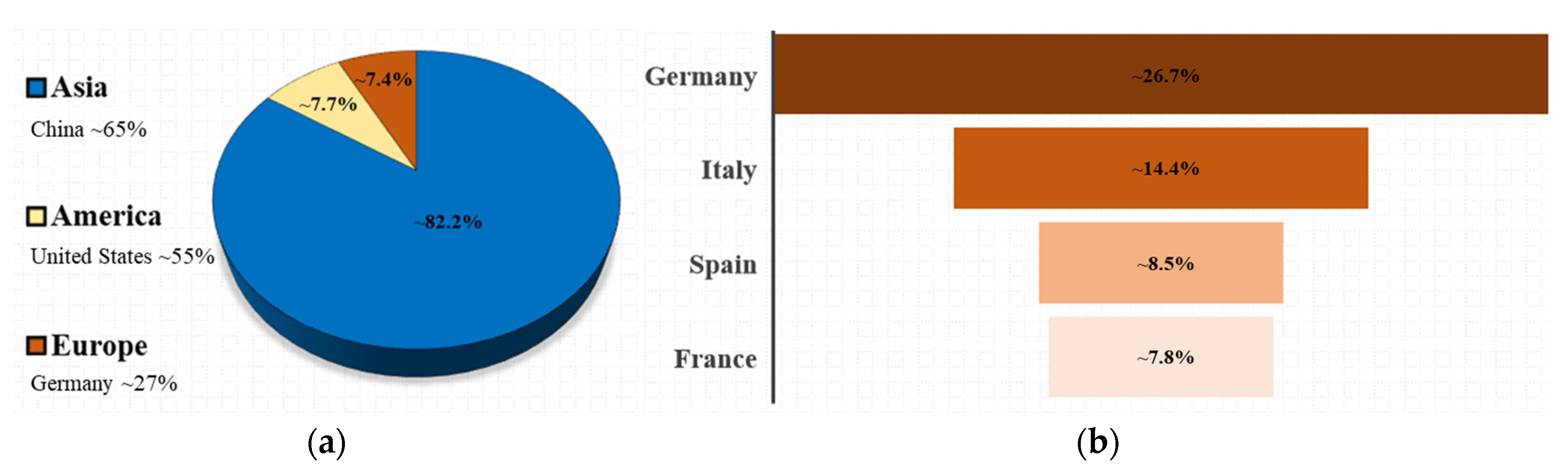
Figure 2.
Test sites: the ArcelorMittal Asturias steel plants (a) Gijón and (b) Avilés. White polygons indicate the main sub-assets responsible for the steelmaking process: 11 for Gijón and 8 for Avilés.
Figure 2.
Test sites: the ArcelorMittal Asturias steel plants (a) Gijón and (b) Avilés. White polygons indicate the main sub-assets responsible for the steelmaking process: 11 for Gijón and 8 for Avilés.
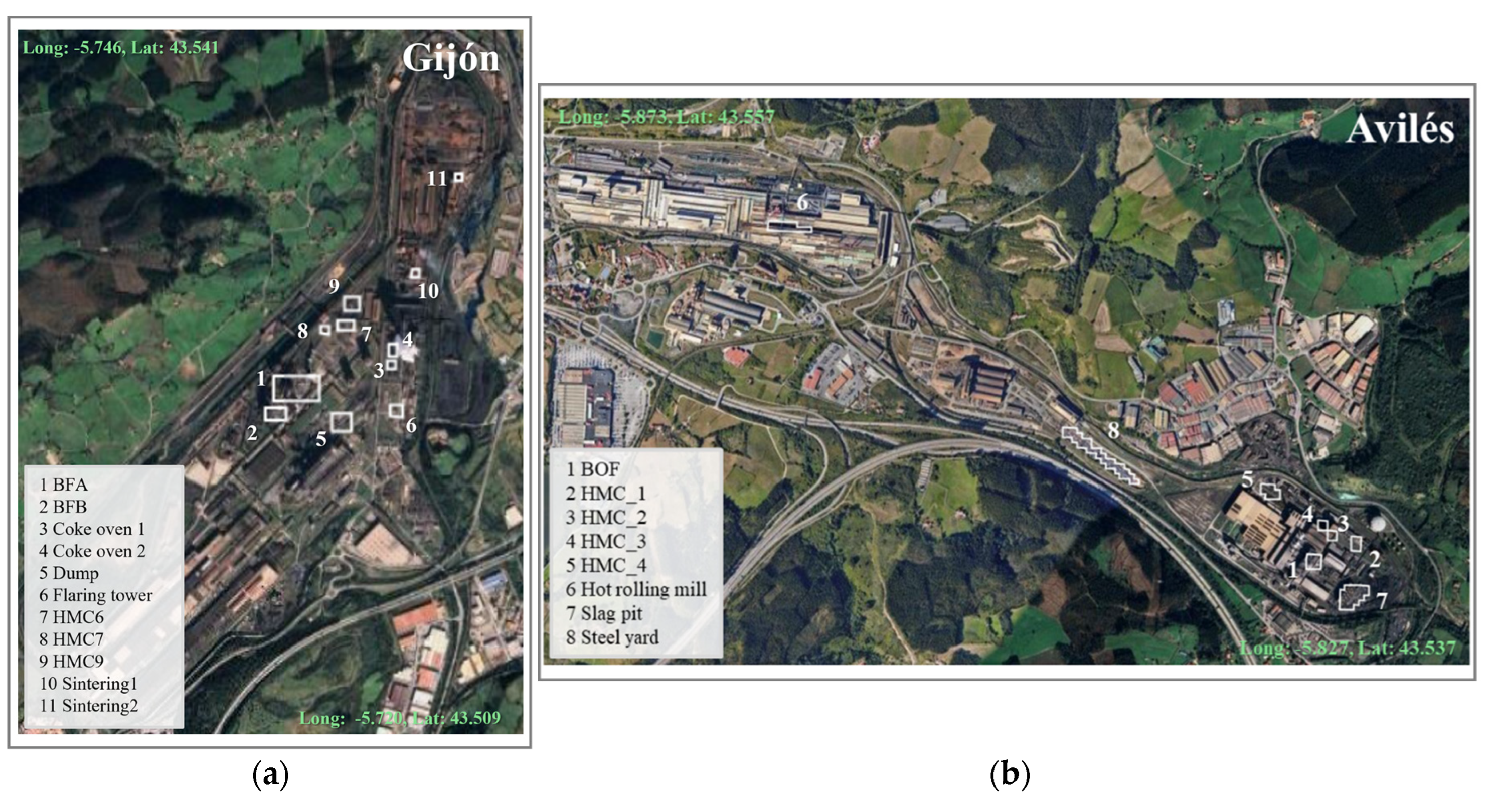
Figure 3.
(a) The false color MSI image (R: B12, G: B11, B: B8A) acquired on 29 January 2022 over Gijón used to plot satellite signals/metrics; (b) Reflectance/TAI (top) and radiance/NHI (bottom) profiles along the white transect shown in the left image, crossing hot industrial sub-assets (dump and flaring tower, numbers 5 and 6 in Figure 2a).
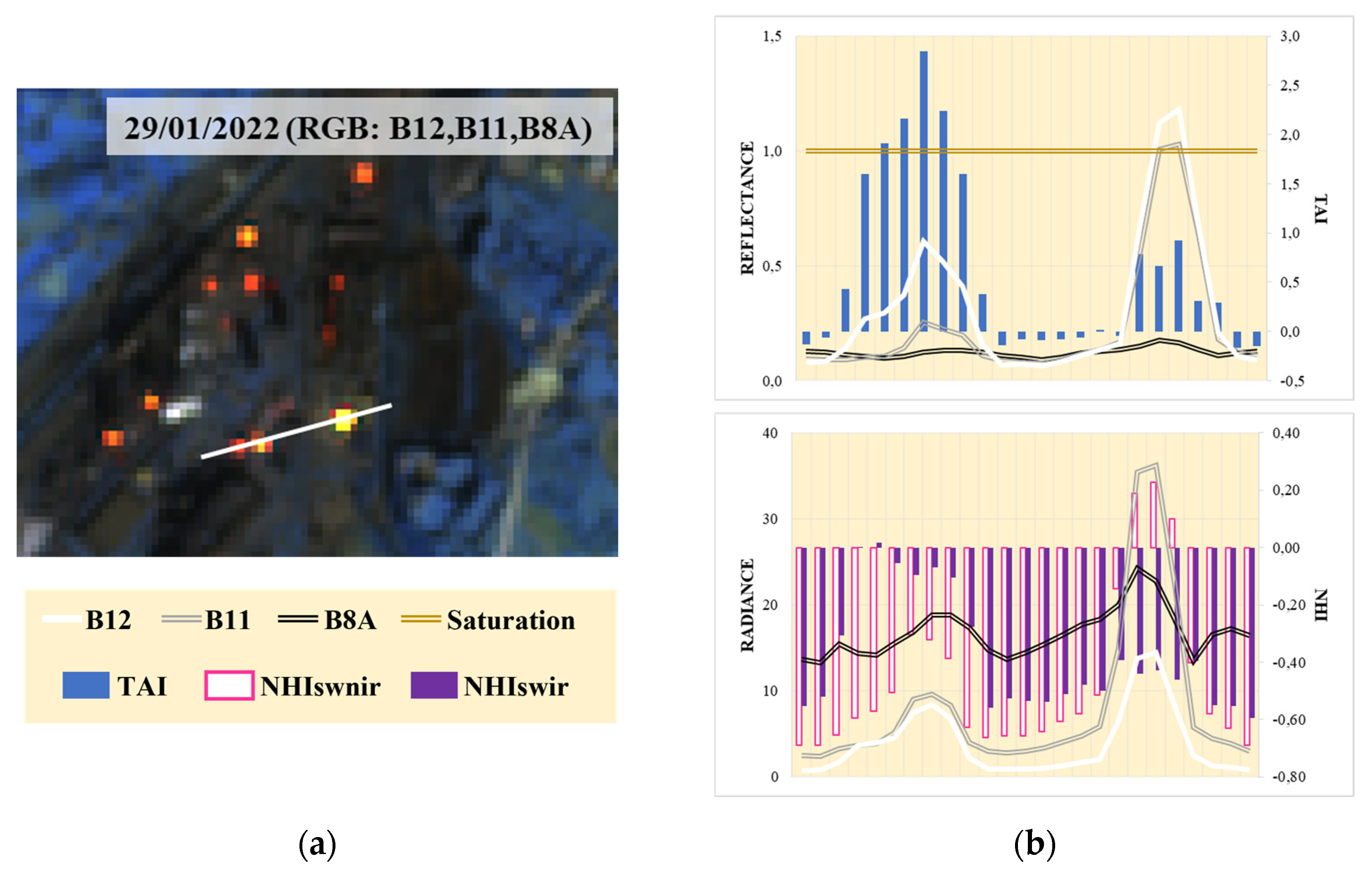
Figure 4.
(a) The false color MSI image (R: B12, G: B11, B: B8A) acquired on 17 September 2018 over Avilés used to plot satellite signals/metrics; (b) reflectance/TAI (bottom left) and radiance/NHI (bottom right) profiles along the black transect in the top image crossing hot industrial sub-assets (BOF and slag pit, numbers 1 and 7 in Figure 2b).
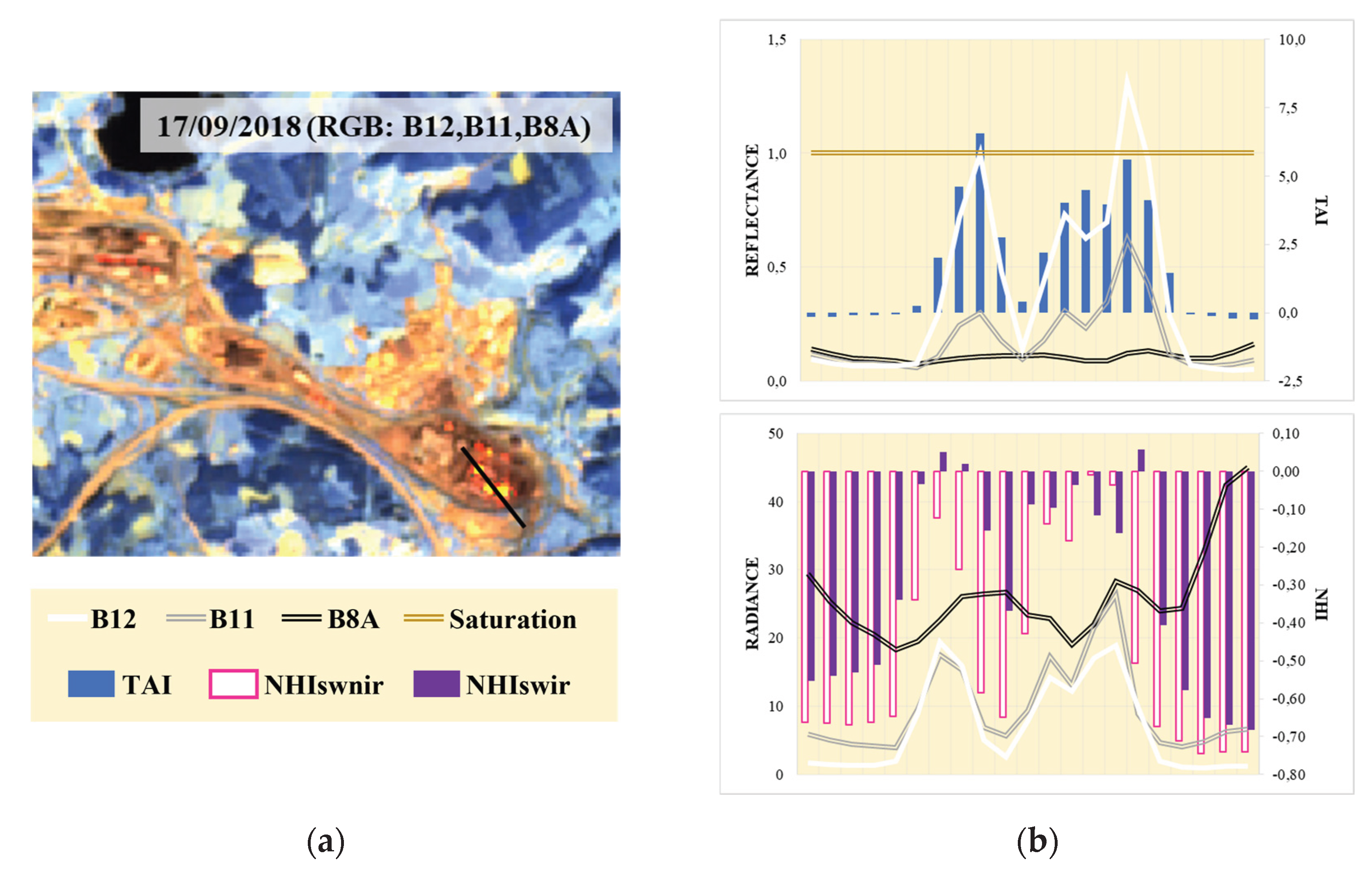
Figure 5.
Hot pixels scatter density in the spectral characteristic of SWIR2, SWIR1 and NIR for (a) TAI; (b) NHIswir; (c) NHIswnir. Hot pixels are the ones in Gijón and Avilés sub-assets. Grey dots represent cloudy pixels.
Figure 5.
Hot pixels scatter density in the spectral characteristic of SWIR2, SWIR1 and NIR for (a) TAI; (b) NHIswir; (c) NHIswnir. Hot pixels are the ones in Gijón and Avilés sub-assets. Grey dots represent cloudy pixels.
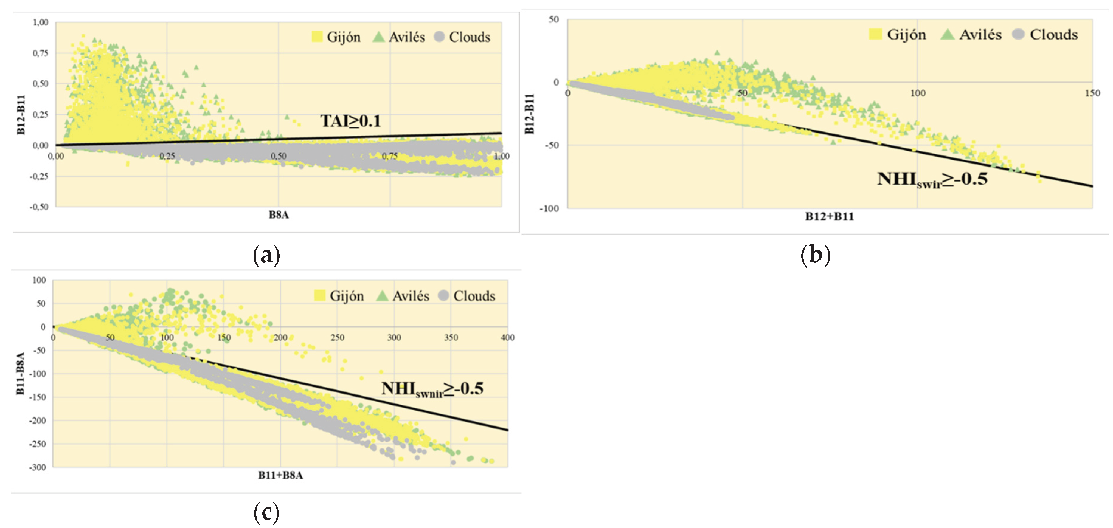
Figure 6.
Ground-truth production data for Spain from EF and WSA: crude steel production is shown by black bars (WSA) and black dotted lines (EF), while pig iron production is represented by the grey line, covering the years 2020–2023. Production values are allocated with 22% attributed to Gijón and 78% to Avilés.
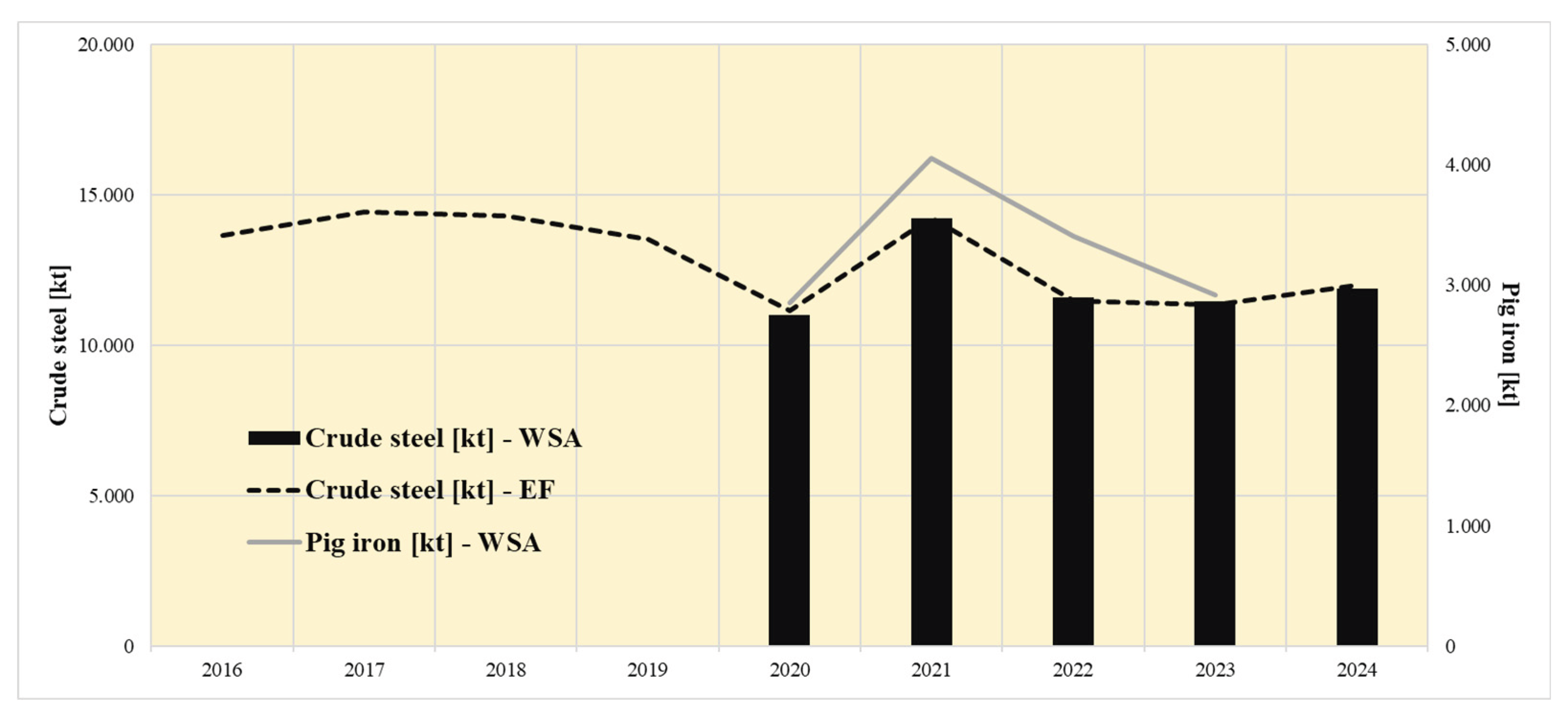
Figure 7.
Flowchart of the methodological scheme developed for TAI (left panel) and NHIs (right panel) metrics.
Figure 7.
Flowchart of the methodological scheme developed for TAI (left panel) and NHIs (right panel) metrics.
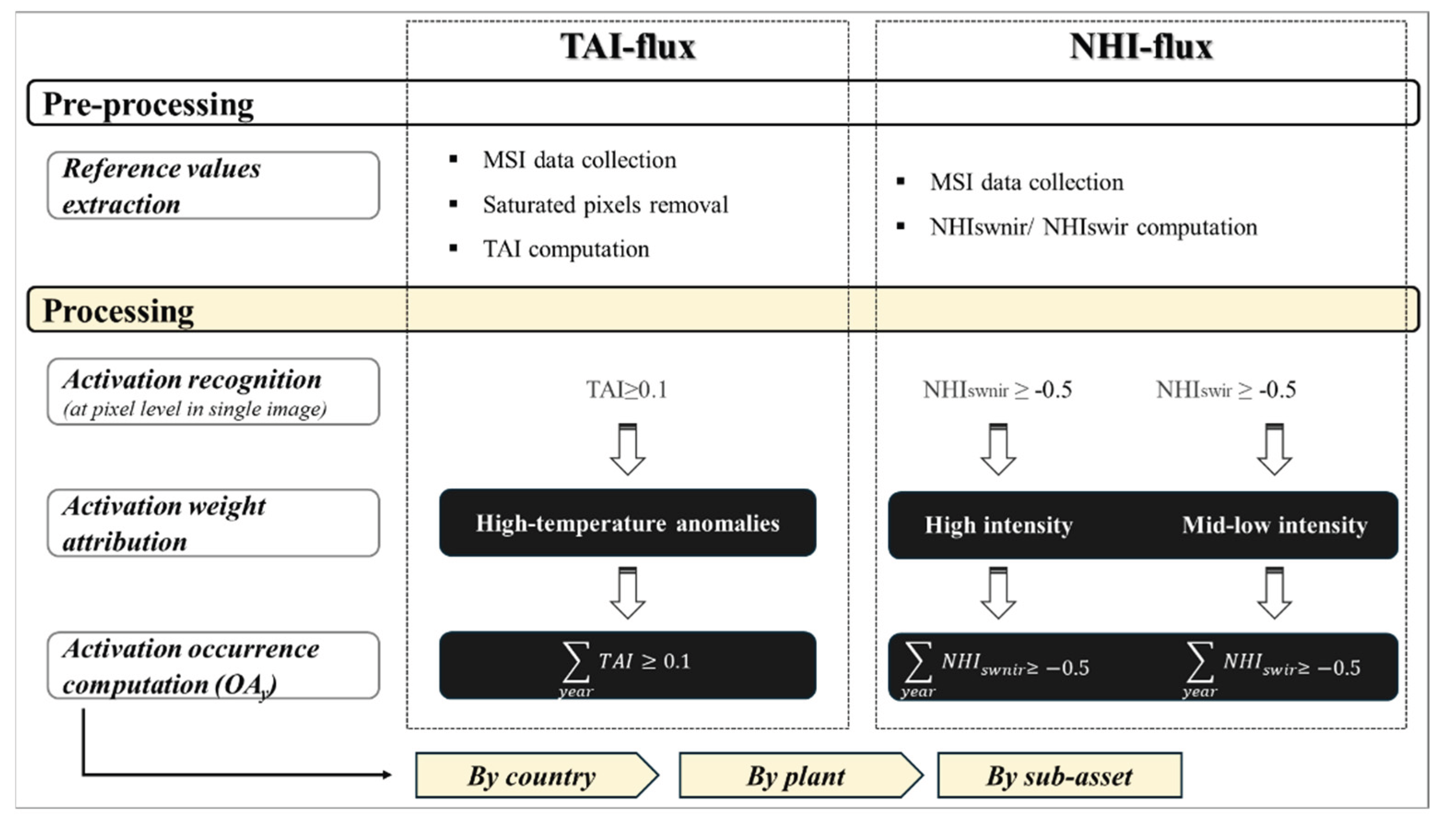
Figure 8.
Linear regression models for (a) crude steel production by EF (2016˗2024); (b) crude steel by WSA (2020˗2024); (c) pig iron (2020˗2023). Each graph includes samples and linear regression equations for TAI (blue dots), NHIswnir (purple rhombi) and NHIswir (pink squares).
Figure 8.
Linear regression models for (a) crude steel production by EF (2016˗2024); (b) crude steel by WSA (2020˗2024); (c) pig iron (2020˗2023). Each graph includes samples and linear regression equations for TAI (blue dots), NHIswnir (purple rhombi) and NHIswir (pink squares).
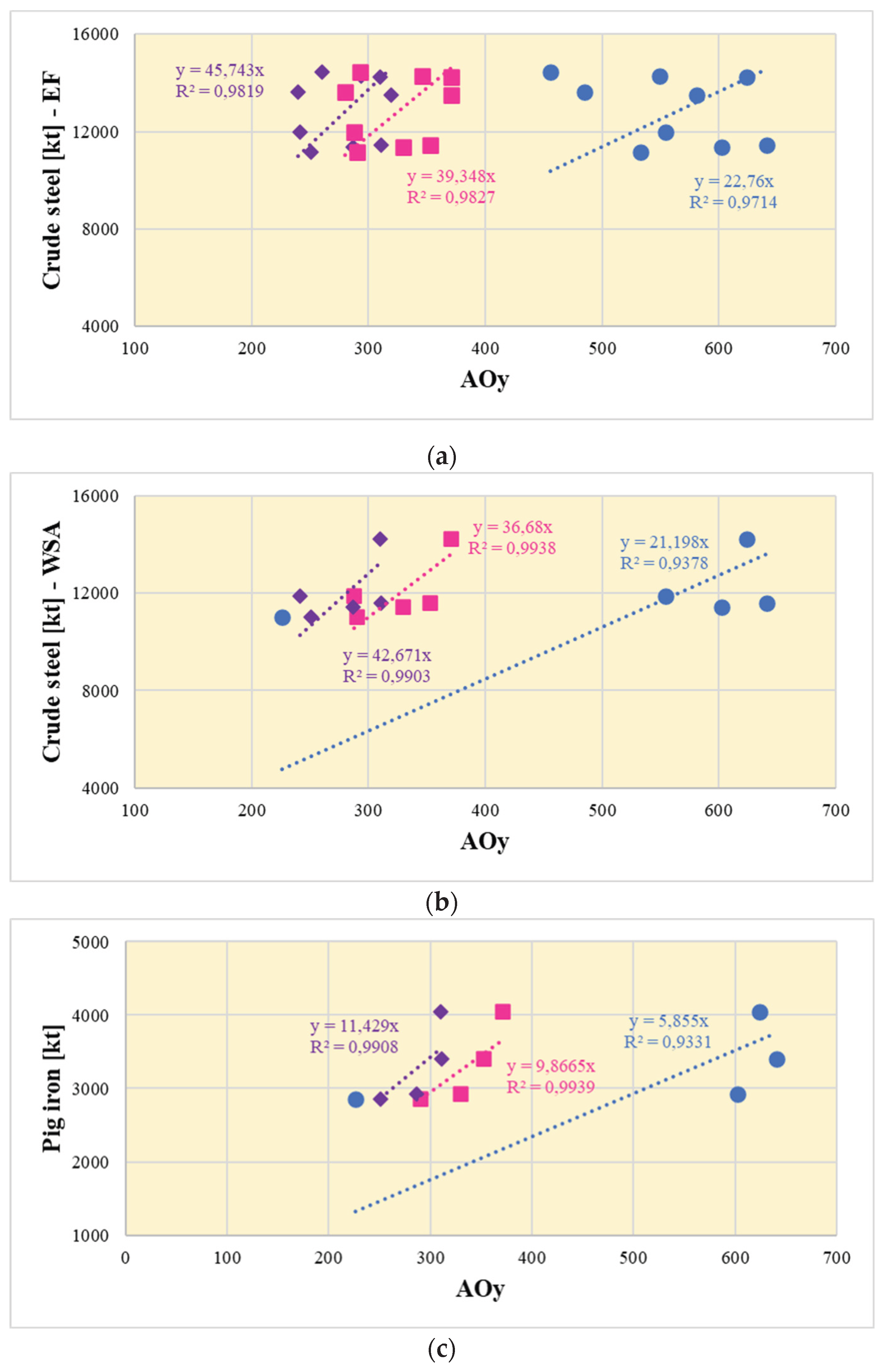
Figure 9.
Occurrence of activations for (a) TAI≥0.1; (b) NHIswnir≥-0.5; (c) NHIswir≥-0.5 over Gijón (left) and Avilés (right). Black polygons delineate the investigated sub-assets involved in the steelmaking process (11 for Gijón and 8 for Avilés, see Figure 2).
Figure 9.
Occurrence of activations for (a) TAI≥0.1; (b) NHIswnir≥-0.5; (c) NHIswir≥-0.5 over Gijón (left) and Avilés (right). Black polygons delineate the investigated sub-assets involved in the steelmaking process (11 for Gijón and 8 for Avilés, see Figure 2).
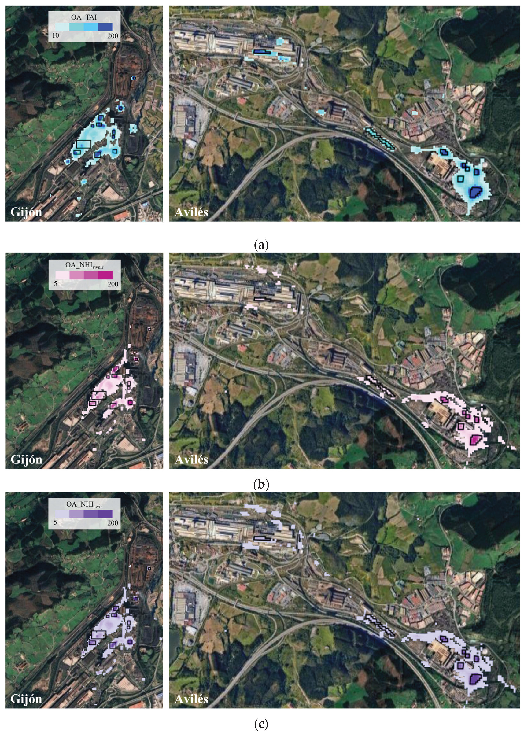
Figure 10.
Annual percentage of activations recorded for Gijón sub-assets (a) coke oven 1; (b) coke oven 2; (c) flaring tower and (d) sintering 2. Activations are shown for TAI (blue line) and NHIs (pink line for NHIswnir, purple line for NHIswir) over the period 2016˗2024. The table in the top-left corner quantifies the percentage of activations by metric type.
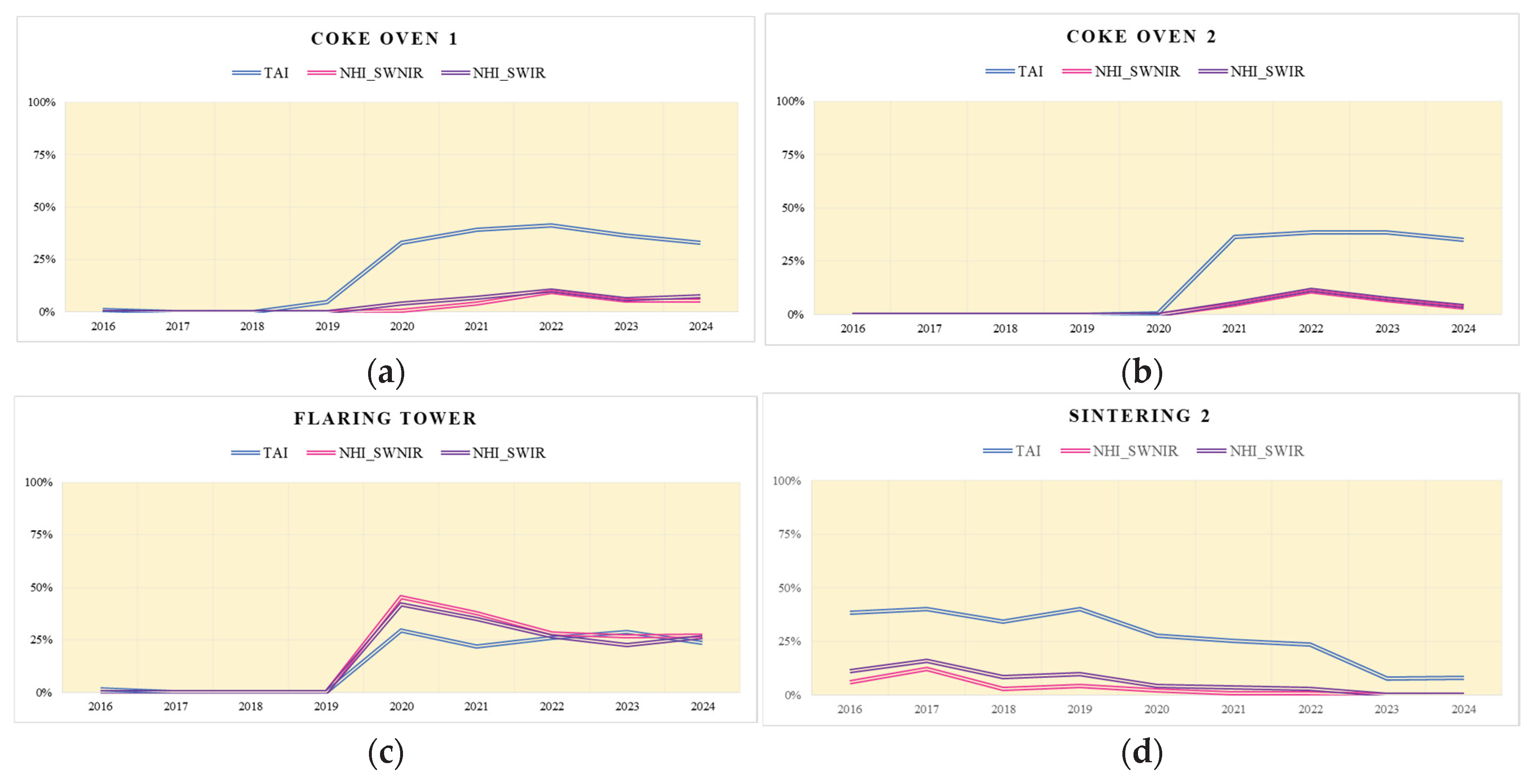
Figure 11.
Maps showing activations recorded for (a) BFA and (b) BOF by TAI and NHIs during the period 2016˗2024. The tables below summarize the comparison between the mean R2 values obtained from the individual indices and those derived from the blended system.
Figure 11.
Maps showing activations recorded for (a) BFA and (b) BOF by TAI and NHIs during the period 2016˗2024. The tables below summarize the comparison between the mean R2 values obtained from the individual indices and those derived from the blended system.
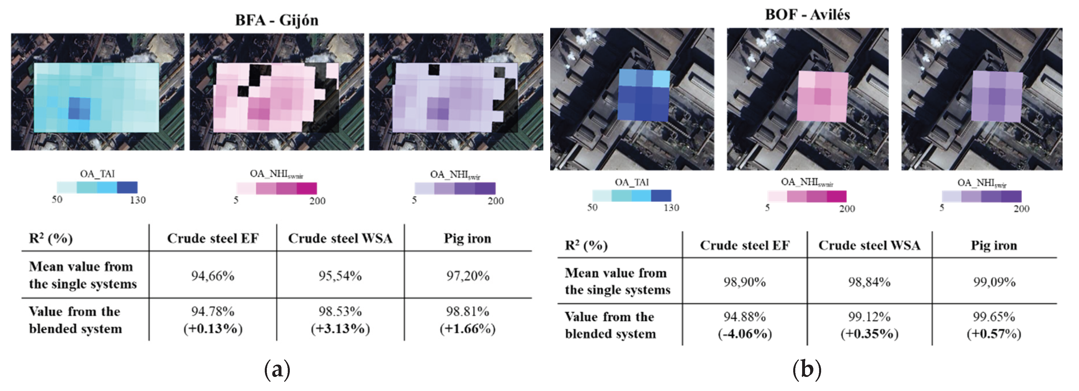
Figure 12.
Number of activations recorded for BFA (black line) and BOF (grey line) using the blended system over 2016–2024.
Figure 12.
Number of activations recorded for BFA (black line) and BOF (grey line) using the blended system over 2016–2024.
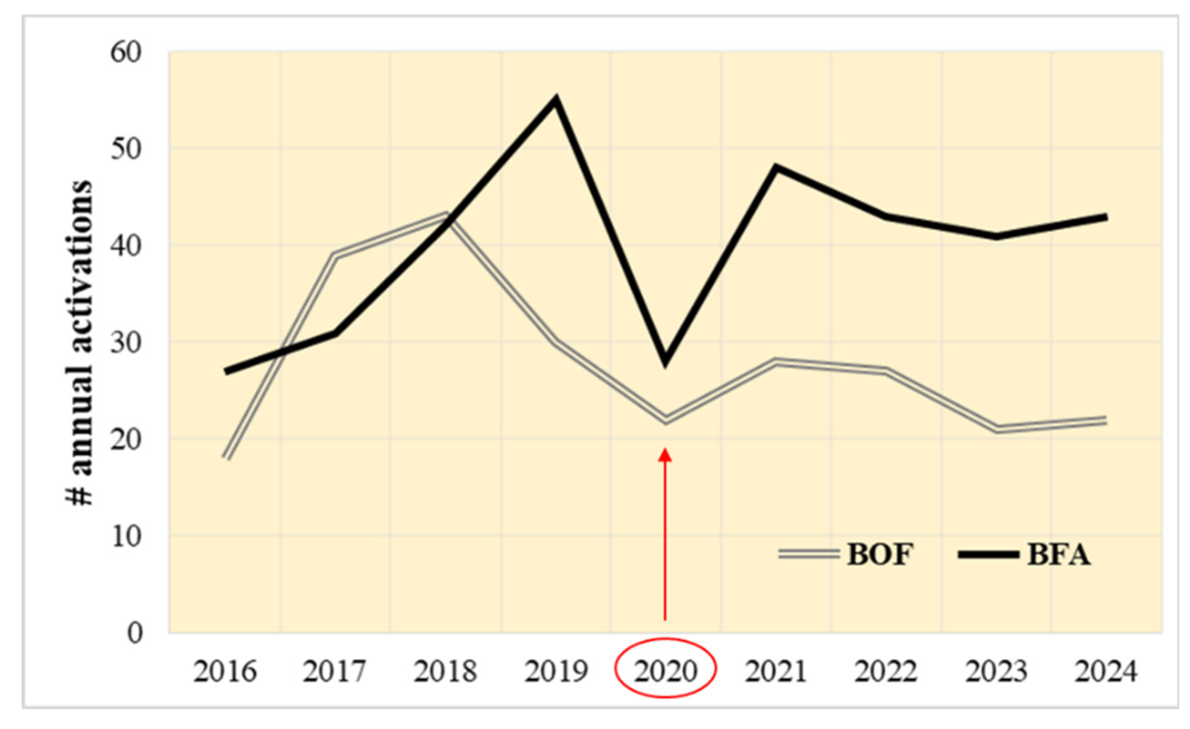
Figure 13.
Monthly activation trends of a) BFA and b) BOF in 2020 (black histogram) and 2024 (white histogram filled with black dots), as derived from the integrated satellite system.
Figure 13.
Monthly activation trends of a) BFA and b) BOF in 2020 (black histogram) and 2024 (white histogram filled with black dots), as derived from the integrated satellite system.
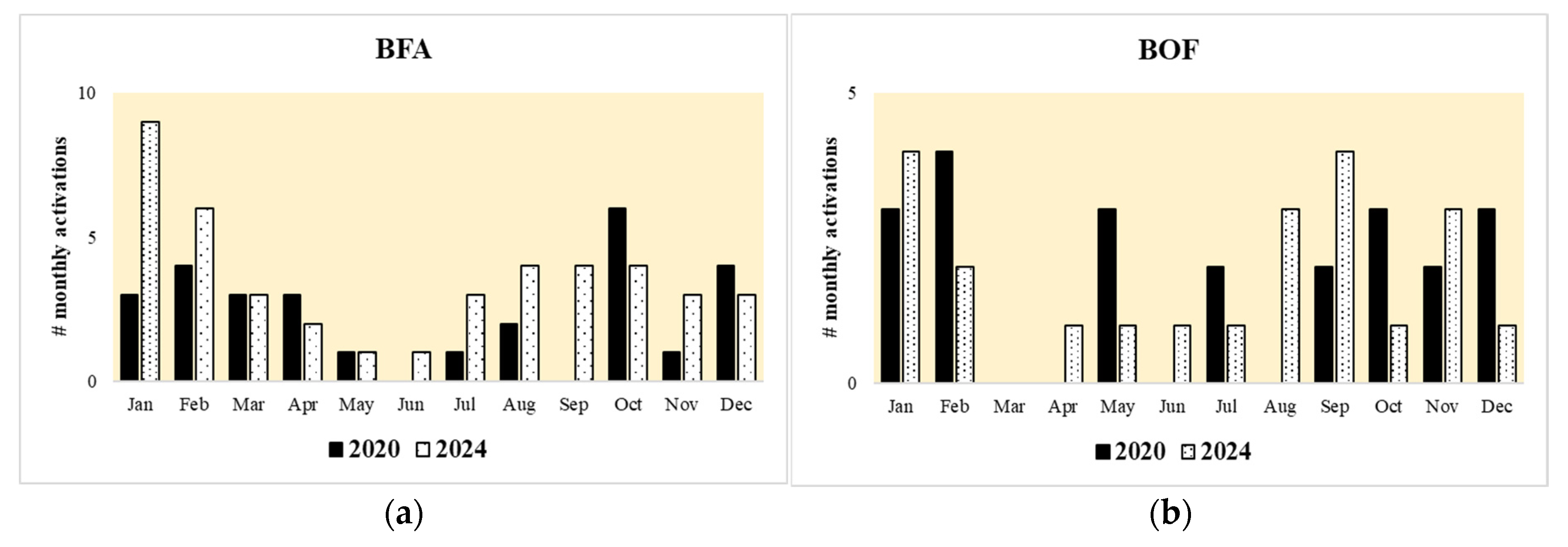

Table 1.
Literature papers on industrial sites investigation by satellite data.
| Paper reference | Study area |
Satellite sensor |
Spectral bands | Pixel size (m) | Parameter | Observational conditions | Temporal window |
|---|---|---|---|---|---|---|---|
| [14] | Global | VIIRS | DNB, NIR, M7, M8, M10, M12, M13 | 750 | VNF | Nighttime | 2012–2016 |
| [24] | China | TIRS | LWIR-1, LWIR-2 | 100 | LST | Daytime | 2013–2017 |
| [25] | China | ASTER | BT10, BT11, BT12, BT13, BT14 | 90 | TAI* | Nighttime | 2016–2017 |
| [32] | China | VIIRS | I4 | 375 | BT MVC | Nighttime | 2018 |
| [26] | China | VIIRS | I4, I5 | 375 | VNP14IMG | Daytime &Nighttime | 2016 |
| [16] | Global | MSI | B8A, B11, B12 | 20 | TAI** | Daytime | 2016–2018 |
| [15] | Malaysia | OLI, TIRS | B4-B5-B6, B10-B11 | 30/100 | NDVI, NDBI, NDSI | Daytime | 2020 |
| [27] | China | VIIRS | 375 | VNP14IMG | Daytime | 2013–2019 | |
| [8] | China | VIIRS, OLI | 750,375,30 | VNF, VIIRS&L8 Fires products | Daytime | 2012–2020 | |
| [9] | China | TIRS | B10-B11 | 100 | LST | Daytime | 2013–2017 |
| [28,29,30,31] | Global | OLI/MSI | B5-B6-B7, B8A-B11-B12 | 30/20 | NHI | Daytime | 2013–2023 |
TAI highlighted with * (single asterisk) and ** (double asterisk) refer to different formulas. For details, see the original papers.
Table 2.
R2 between satellite-derived metrics (TAI, NHIswnir, NHIswir) and crude steel (EF, WSA) and pig iron production.
Table 2.
R2 between satellite-derived metrics (TAI, NHIswnir, NHIswir) and crude steel (EF, WSA) and pig iron production.
| Site | R2 (%) | Crude steel EF (2016˗2024) |
Crude steel WSA (2020˗2024) |
Pig iron (2020 ˗2023) |
|---|---|---|---|---|
| Gijón | TAI | 94.88 | 99.34 | 99.06 |
| NHIswnir | 97.31 | 98.96 | 99.63 | |
| NHIswir | 97.76 | 99.24 | 99.81 | |
| Avilés | TAI | 98.15 | 98.19 | 97.15 |
| NHIswnir | 97.73 | 98.27 | 97.26 | |
| NHIswir | 97.96 | 98.86 | 98.08 |
Table 3.
R2 values for Gijón sub-assets, estimated using TAI occurrences.
| R2 (%) | Crude steel EF (2016˗2024) |
Crude steel WSA (2020˗2024) |
Pig iron (2020 ˗2023) |
|---|---|---|---|
| BFA | 94.66 | 95.54 | 97.20 |
| BFB | 91.89 | 94.14 | 91.68 |
| Coke oven 1 | 50.93 | 99.09 | 98.88 |
| Coke oven 2 | 39.91 | 83.03 | 80.57 |
| Dump | 98.41 | 99.07 | 98.93 |
| Flaring tower | 47.61 | 96.24 | 93.63 |
| HMC6 | 98.65 | 97.93 | 97.44 |
| HMC7 | 97.80 | 96.36 | 94.00 |
| HMC9 | 97.77 | 97.76 | 95.08 |
| Sintering 1 | 92.74 | 87.89 | 86.79 |
| Sintering 2 | 89.13 | 96.47 | 89.44 |
Table 4.
As Table 3 for NHIswnir occurrences.
Table 4.
As Table 3 for NHIswnir occurrences.
| R2 (%) | Crude steel EF (2016˗2024) |
Crude steel WSA (2020˗2024) |
Pig iron (2020 ˗2023) |
|---|---|---|---|
| BFA | 92.90 | 92.54 | 92.41 |
| BFB | 96.10 | 98.13 | 96.79 |
| Coke oven 1 | 36.08 | 75.21 | 72.64 |
| Coke oven 2 | 32.06 | 67.07 | 69.35 |
| Dump | 98.30 | 99.02 | 99.17 |
| Flaring tower | 45.99 | 94.93 | 93.43 |
| HMC6 | 96.30 | 94.44 | 95.83 |
| HMC7 | 94.24 | 97.22 | 94.89 |
| HMC9 | 92.13 | 93.13 | 93.63 |
| Sintering 1 | 89.73 | 81.94 | 87.77 |
| Sintering 2 | 54.33 | 43.10 | 52.19 |
Table 5.
As Table 3 for NHIswir occurrences.
Table 5.
As Table 3 for NHIswir occurrences.
| R2 (%) | Crude steel EF (2016˗2024) |
Crude steel WSA (2020˗2024) |
Pig iron (2020 ˗2023) |
|---|---|---|---|
| BFA | 94.66 | 94.85 | 94.86 |
| BFB | 97.67 | 99.33 | 97.88 |
| Coke oven 1 | 44.47 | 92.27 | 92.26 |
| Coke oven 2 | 33.15 | 69.31 | 70.74 |
| Dump | 98.20 | 98.76 | 99.40 |
| Flaring tower | 45.95 | 94.83 | 93.20 |
| HMC6 | 96.48 | 94.71 | 95.65 |
| HMC7 | 97.21 | 97.20 | 94.74 |
| HMC9 | 93.00 | 97.82 | 97.40 |
| Sintering 1 | 91.85 | 85.85 | 87.74 |
| Sintering 2 | 70.70 | 59.89 | 75.59 |
Table 6.
R2 values for Avilés sub-assets, estimated using TAI occurrences.
| R2 (%) | Crude steel EF (2016˗2024) |
Crude steel WSA (2020˗2024) |
Pig iron (2020 ˗2023) |
|---|---|---|---|
| BOF | 98.90 | 98.84 | 99.07 |
| HMC1 | 95.21 | 92.18 | 91.12 |
| HMC2 | 97.15 | 97.97 | 96.68 |
| HMC3 | 97.01 | 97.78 | 95.88 |
| HMC4 | 92.53 | 98.84 | 95.04 |
| Hot rolling mill | 98.94 | 98.35 | 97.64 |
| Slag pit | 98.00 | 98.27 | 97.57 |
| Steel yard | 85.64 | 92.06 | 98.79 |
Table 7.
As Table 6 for NHIswnir occurrences.
Table 7.
As Table 6 for NHIswnir occurrences.
| R2 (%) | Crude steel EF (2016˗2024) |
Crude steel WSA (2020˗2024) |
Pig iron (2020 ˗2023) |
|---|---|---|---|
| BOF | 93.90 | 95.53 | 96.19 |
| HMC1 | 87.88 | 80.36 | 74.61 |
| HMC2 | 90.97 | 90.36 | 87.24 |
| HMC3 | 94.50 | 95.00 | 97.89 |
| HMC4 | 91.12 | 92.64 | 93.32 |
| Hot rolling mill | 67.38 | 52.21 | 64.39 |
| Slag pit | 96.27 | 97.65 | 97.01 |
| Steel yard | 70.73 | 90.78 | 90.75 |
Table 8.
As Table 6 for NHIswir occurrences.
Table 8.
As Table 6 for NHIswir occurrences.
| R2 (%) | Crude steel EF (2016˗2024) |
Crude steel WSA (2020˗2024) |
Pig iron (2020 ˗2023) |
|---|---|---|---|
| BOF | 98.49 | 97.73 | 99.09 |
| HMC1 | 88.94 | 84.46 | 81.01 |
| HMC2 | 91.40 | 91.16 | 88.83 |
| HMC3 | 94.79 | 97.05 | 98.34 |
| HMC4 | 90.11 | 91.55 | 91.79 |
| Hot rolling mill | 92.52 | 88.79 | 86.03 |
| Slag pit | 96.36 | 98.63 | 98.38 |
| Steel yard | 82.61 | 89.30 | 98.15 |
Table 9.
Ranking of sub-assets based on the satellite blended system.
| Rank | Gijón | R2 (%) | Avilés | R2 (%) |
|---|---|---|---|---|
| #1 | Dump | 98.21 | BOF | 97.11 |
| #2 | HMC6 | 96.71 | Slag pi | 97.08 |
| #3 | HMC7 | 95.83 | HMC3 | 95.39 |
| #4 | BFB | 95.45 | HMC2 | 93.21 |
| #5 | BFA | 94.23 | HMC4 | 92.23 |
| #6 | HMC9 | 93.78 | HMC1 | 89.66 |
| #7 | Sintering 1 | 90.68 | Hot rolling mill | 86.74 |
| #8 | Sintering 2 | 72.24 | Steel yard | 82.72 |
| #9 | Flaring tower | 57.26 | ||
| #10 | Coke oven 1 | 54.51 | ||
| #11 | Coke oven 2 | 44.39 |
Table 10.
Model parameters for Spain derived from TAI, NHIswnir and NHIswir.
| Spanish BF/BOF plants | TAI | NHIswnir | NHIswir |
|---|---|---|---|
| Linear regression model 2016-2023 | y=22.89x (R2=96.87%) |
y=45.38x (R2=98.08%) |
y=39.13x (R2=98.12%) |
| Crude steel 2024 EF [kt] | 11997 | ||
| Model-estimated value | 12683 | 10937 | 11269 |
| (+/–) deviation from the expected value | +5.7% | -8.8% | -6.1% |
Table 11.
As Table 10 for France.
Table 11.
As Table 10 for France.
| French BF/BOF plants | TAI | NHIswnir | NHIswir |
|---|---|---|---|
| Linear regression model 2016-2023 | y=86,75x (R2=96.63%) |
y=119,16x (R2=96.86%) |
y=105,27x (R2=97.20%) |
| Crude steel 2024 EF [kt] | 10753 | ||
| Model-estimated value | 12319 | 11082 | 10738 |
| (+/–) deviation from the expected value | +14.6% | +3.1% | +0.1% |
Table 12.
As Table 10 for Germany.
Table 12.
As Table 10 for Germany.
| German BF/BOF plants | TAI | NHIswnir | NHIswir |
|---|---|---|---|
| Linear regression model 2016-2023 | y=123,91x (R2=96.14%) |
y=197,81x (R2=94.84%) |
y=147,84x (R2=94.71%) |
| Crude steel 2024 EF [kt] | 37234 | ||
| Model-estimated value | 31597 | 31847 | 32525 |
| (+/–) deviation from the expected value | -15.1% | -14.5% | -12.6% |
Disclaimer/Publisher’s Note: The statements, opinions and data contained in all publications are solely those of the individual author(s) and contributor(s) and not of MDPI and/or the editor(s). MDPI and/or the editor(s) disclaim responsibility for any injury to people or property resulting from any ideas, methods, instructions or products referred to in the content. |
© 2026 by the authors. Licensee MDPI, Basel, Switzerland. This article is an open access article distributed under the terms and conditions of the Creative Commons Attribution (CC BY) license (http://creativecommons.org/licenses/by/4.0/).
Copyright: This open access article is published under a Creative Commons CC BY 4.0 license, which permit the free download, distribution, and reuse, provided that the author and preprint are cited in any reuse.


