
Submitted:
12 February 2026
Posted:
13 February 2026
You are already at the latest version
Abstract
A laboratory–scale mechanical draft cooling tower equipped with eight sections of perforated inclined plates was designed to determine the effect of operating conditions on the volumetric mass transfer coefficient (kya) between water and air. A three–factor, three–level design of experiments (DOE) was implemented, considering liquid mass flow rate L (120, 240, and 360 kg/h), gas mass flow rate G (36, 57, and 75 kg/h), and top water temperature TL2 (50, 60, and 70◦C). A total of 54 runs were performed, and the global volumetric mass transfer coefficient was calculated by combining energy and mass balances with the Mickley method. The experimental data were fitted to a power–law correlation using multivariable regression. The ANOVA showed that TL2 is the dominant factor, followed by L, whereas the influence of G is comparatively small in the studied range. The selected correlation, based on the nominal gas flow rate, achieved R2=0.869 and a RMSE of 5930 kg/(m3h). The kya values were found in the range from 4600 to 62000 kg/(m3h). Vertical temperature profiles of water and air along the column revealed that, for high liquid flow rates, most of the cooling occurs in the lower stages, suggesting that the upper sections are underutilized.
Keywords:
laboratory-scale cooling tower
; evaporative cooling
; volumetric mass transfer coefficient
; operating conditions
; perforated inclined plates
1. Introduction
Cooling towers are one of the key components in industries, mainly used with the purpose of decreasing the temperature of hot liquids. In the case of the thermoelectric generation industry, the required cooling is responsible for approximately 10% of the total water demand in the world [1]. Their performance depends on coupled heat and mass transfer between a warm water stream and ambient air; also, it is strongly influenced by tower geometry, fill characteristics, and operating conditions [2,3,4]. In addition, cooling water management and environmental constraints related to biofouling, plume formation, blowdown, and pressure drop further motivate the improvement of tower efficiency [5].
Since the groundbreaking work of Merkel [6], several modelling approaches have been proposed, ranging from the classical Merkel integral and Poppe-type models to effectiveness– NTU formulations and detailed numerical simulations [7,8,9,10]. Many experimental studies on pilot and industrial towers have explored the influence of liquid and gas flow rates, water temperature, fill type, and number of stages on tower performance and on the volumetric mass transfer coefficient kya [2,3,11,12,13,14,15]. Other works have focused on packing arrangement, pressure drop, and the development of semi-empirical correlations for performance evaluation under irregular ambient conditions [10,16,17,18,19,20].
Recently, the development of new fill materials and alternative contact devices has gained relevance due to the need to improve efficiency, reduce water consumption, and mitigate fouling [4]. Studies have addressed different film and splash fills, as well as structured packings that change the hydrodynamics of the water film [17,19,21]. Controlled laboratory towers are particularly valuable to test unconventional fills and to obtain high–quality data for correlation development. However, most works still focus on classical fills, while alternative geometries such as perforated inclined plates remain less explored.
Optimization of circulating cooling water systems is becoming increasingly important in the context of energy efficiency and decarbonization initiatives [22,23,24,25,26,27,28]. Accurate and robust correlations for kya are essential inputs for such optimization frameworks, particularly when combined with process simulation and data-driven statistical models [22,28,29]. These correlations must reflect not only geometric characteristics but also the sensitivity of mass transfer to operating conditions, so that operating conditions can be optimized without losing cooling performance.
The present work contributes to this context by providing new experimental information for a laboratory–scale mechanical draft cooling tower equipped with acrylic perforated inclined plates. The purpose is to quantify the effect of liquid mass flow rate L, gas mass flow rate G, and top water temperature TL2 on the global volumetric mass transfer coefficient kya, and to develop an empirical correlation valid within the experimental range. A three–factor, three–level design of experiments (DOE) was carried out, and the data were analyzed using ANOVA, following strategies commonly applied in cooling-tower optimization and grounded in standard DOE methodology [14,15,30,31,32]. In addition, the distribution of heat transfer by section along the column was evaluated to understand how operating conditions modify the internal thermal behavior of the tower.
2. Materials and Methods
2.1. Experimental Facility
Experiments were run in a counterflow mechanical–draft cooling tower located at the Heat and Mass Transfer Laboratory of Universidad del Atlántico, see figure 1. The column was built in transparent acrylic, which allows visual inspection of the flow, and was divided into eight identical stages, which had perforated inclined plates. Each plate was mounted at a fixed angle with respect to the horizontal and perforated with uniformly distributed circular holes to enhance the air– water contact. The design and hydrodynamic characterization of similar units have been reported in previous works [33,34,35].
Warm water from a storage tank (see figure 1) was pumped by a multistage centrifugal pump (P–101) to the top of the column, where it was distributed through the top plate. Water flows down by gravity through all the stages and is collected at the bottom in a container. Ambient air was supplied by a centrifugal blower (K–101) and introduced at the base of the column, where it flowed upward in counter-current to the water stream. The air flow rate was changed by a variable–frequency drive (VFD–101) installed on the blower.
Water temperatures were measured at the inlet and outlet of the column and at intermediate heights using calibrated Pt100 resistance thermometers with an uncertainty of ±0.1 ◦C. Air dry–bulb temperature and relative humidity at the inlet and outlet are measured with similar Pt100 sensors. All the measures were used to determine the air enthalpy and humidity ratio via psychrometric relationships [36,37]. Liquid and gas flow rates were determined by a flowmeter and an anemometer, respectively. All signals were reported through a data acquisition system and recorded once the steady state was reached.
2.2. Design of Experiments
The effect of the operating conditions on the global volumetric mass transfer coefficient kya was studied considering a three–factor, three–level, two-replicate design of experiments resulting in 27 distinct combinations and a total of 54 experiments. The selected factors, shown in Table 1, were liquid mass flow rate L; gas mass flow rate G; and top water temperature TL2. The levels were chosen based on preliminary tests and on the hydraulic and thermal limitations of the experimental setup, following standard DOE principles [31,32].
The system reached steady state for each experiment (based on stable temperatures and flow rates). Figure 3 illustrates the experimental domain in the L–G–TL2 space. The selected levels ensure that flooding or severe entrainment did not occur.
2.3. Thermodynamic Framework and Calculation of kya
The analysis is based on Merkel's classical approach, which combines sensible and latent heat transfer in a single process that is controlled by mass transfer [6,7,38]. For a differential height dZ in a completely irrigated counterflow tower, the energy balance between the water and the air can be written as:
where Gs′ is the dry–air mass flux, hy and hyi are the dry and interfacial humid air enthalpies, TL and Ti are the bulk liquid and interfacial temperatures, hL is the liquid heat transfer convective coefficient, and a is the specific surface area per unit volume [39,40].
Assuming that the liquid is well distributed in each section and using appropriate property correlations for water and humid air [36,37], overall energy balances between the inlet and outlet of the tower provide the total heat transfer rate in the column. Mickley's graphical method, which is used to plot the temperature and enthalpy profiles of the gas along the column, is combined with the Merkel method to determine the overall volumetric mass transfer coefficient kya shown in equation (2), [3,9].
The limits hy,1 and hy,2 correspond to the inlet and outlet air enthalpies, respectively.
For each operating condition, a Mickley diagram was developed by dividing the column into 98 equal sections and performing enthalpy balances, which yielded a set of points (hy, hyi). This approach allowed the integral of the Merkel equation to be solved using numerical methods, resulting in equation (3):
This expression was used to compute the overall volumetric mass transfer coefficient using the experimental air enthalpies and the fitted parameters A and B for each experiment.
2.4. Temperature Profiles along the Column
Since the Mickley method links the enthalpy of moist air to its temperature, the air temperature variation along the column was plotted as a function of height. A similar procedure was applied to determine the water temperature profile, allowing a direct comparison of the thermal behavior of both streams along the column. [36,37].
Temperature profiles were obtained for gas flow rate G = 36, 57, and 75 kg/h and top water temperature TL2 = 50, 60, and 70°C, keeping the liquid mass flow rate within the range L = 120–360 kg/h.
2.5. Psychrometric Representation and Temperature-Enthalpy Profiles
In addition to the vertical temperature profiles, the evolution of the air-water contact along the column was analyzed on a psychrometric temperature-enthalpy diagram. The specific enthalpy of humid air, hy, was calculated from the line of operation.
For selected operating conditions, the air states at the inlet and outlet of each stage were represented on a T- hy diagram along with the wet air saturation curve. This diagram is obtained directly from the Mickley method and allows the humidification process of the column along its length to be perfectly observed.
In this work, detailed T-hy profiles are presented for a fixed gas mass flow rate, G=36 kg/h, and three values of the top water temperature TL2 = 50, 60, and 70 °C. For each TL2, the three liquid mass flow rates L=120, 240, and 360 kg/h were considered. These profiles are used to interpret the increase in moisture content of the air and its proximity to saturation under different operating conditions.
2.6. Statistical Analysis and Model Fitting
The experimental design and statistical analysis were carried out using analysis of variance (ANOVA) [31,32]. The following power–law correlation was proposed:
which becomes linear in logarithmic form:
Parameters K, α, β, and γ were estimated via multiple linear regression on equation 5. The model was created with 75% of the experiments. The remaining samples were used as prediction data for the model, and thus, observe the behavior of statistical metrics such as the root mean square error of prediction (RMSE), see equation 6, and R2 using the total data to know the reliability of the model.
where n is the number of observations. The ANOVA was used to evaluate the significance of each factor and to verify the adequacy of the model at a significance level α = 0.05
2.7. Estimation and prediction of Outlet Water Temperature (TL1)
To provide practical applicability to the developed mass transfer model, an additional analysis was carried out to estimate and predict the outlet water temperature (TL1) of the cooling tower. The prediction of TL1 is a key operational variable in cooling tower design and performance evaluation, as it directly reflects the thermal effectiveness of the gas–liquid contact and the influence of operating conditions.
The estimation of TL1 was performed using the previously obtained volumetric mass transfer coefficient (kya) correlation, combined with the energy and mass balance formulation applied along the height of the column. For a given set of operating conditions (liquid mass flow rate L, gas mass flow rate G, and inlet water temperature at the top of the column TL2), the model allows to predict the outlet water temperature.
Experimental measurements of TL1 were obtained for each operating condition and compared with the corresponding model predictions. To quantitatively evaluate the predictive capability of the model, the root mean square error of prediction (RMSEP) was calculated, as well as the root mean square error of cross-validation (RMSECV).
3. Results and discussion
3.1. Behavior of Operating Conditions on kya
To analyze the behavior of the volumetric mass transfer coefficient (kya) more closely, it was plotted as a function of TL2 for different combinations of L and G (see Figure 4 and Figure 5). In Figure 4(a), (b), and (c), the values of kya are presented for different air mass flow rates (36, 57, and 75 kg/h) while keeping the water flow rate fixed in each case. For a given water inlet temperature (TL2), the curves show very similar kya values, indicating that increasing the air flow does not produce significant variations in the mass transfer coefficient within the experimental range. This confirms that the influence of air flow is low compared to the other operating variables, which is consistent with the statistical analysis, where the air flow was the least significant variable.
In Figure 5, the behavior of kya is shown for different water flow rates (120, 240, and 360 kg/h) while keeping the air flow constant. It was found that kya always increases with the liquid flow rate for the same TL2, indicating a positive effect of the water flow on mass transfer. As the water inlet temperature increases, particularly above 60 °C, the curves begin to diverge, and the differences in kya values become more pronounced, reflecting a nonlinear response of the system under conditions of higher thermal energy. At high inlet water temperatures, small variations in the liquid flow produce amplified changes in kya and, therefore, in evaporation. Overall, the results in Figure 5 confirm that TL2 is the variable with the greatest impact, followed by the water flow rate, while the effect of the air flow is minimal within the studied range. Besides, it can be seen in Figure 6 that the behavior of the kya is almost linear with TL2 when G is changed for the different values of L. However, this pattern changes to a nonlinear trend when G is constant.
The range of measured kya values was approximately in the range from 4.6×10³ to 6.2×10⁴ kg/(m3 h), which agreed with the values reported in the literature for laboratory cooling towers with similar conditions [3,16,35]. The trend of kya found in this work is qualitatively similar to that found in towers equipped with film or splash fills, suggesting that perforated inclined plates behave as an effective contact device.
3.2. Temperature Profiles Along the Column
Figure 6, Figure 7 and Figure 8 shows the temperature profiles of water and air along the column height for different gas flow rates. For each G, three subplots are presented corresponding to top water temperatures TL2 = 50, 60, and 70 ◦C, and each subplot includes the three liquid mass flow rates (L = 120, 240, and 360 kg/h).
For G = 36 kg/h (Figure 6), the water temperature generally decreases almost linearly from the inlet to the outlet at L = 120 kg/h, while the air temperature increases almost linearly as well, indicating a uniform thermal driving force along the height of the tower. As L increases to 240 and 360 kg/h, a higher amount of water temperature drop occurs in the lower part of the column, whereas the upper stages exhibit smaller gradients.
A similar behavior is observed for G = 57 and 75 kg/h (Figure 7 and Figure 8). Increasing TL2 amplifies the temperature difference at the bottom of the column, resulting in steeper gradients in the first stages, specifically at the highest liquid flow rate. In all cases, the air temperature rises clearly in the lower sections, and then it tends to have a small variation towards the top, resulting in a rapid uptake of heat and moisture near the water outlet.
At high L and high TL2, most of the cooling is concentrated in the lower part of the column, so the extra packing height in the upper stages is not totally exploited.
3.3. Psychrometric Temperature-Enthalpy Profiles
Figure 9 shows the enthalpy of the gas as a function of the gas temperature (curved lines) and the water temperature (straight lines) for G=36 kg/h at three inlet water temperatures, TL2 = 50, 60, and 70 °C. Each group corresponds to three liquid mass flow rates L=120, 240, and 360 kg/h, plotted together with the equilibrium or saturation line of air (dashed curve). The lowest part of the lines corresponds to the bottom of the column, and the upper part of the lines corresponds to the top.
For TL2 = 50 °C, the operating lines (straight lines) on the T–hy diagram remain relatively far from the saturation line, indicating that the system maintains a strong driving force for both heat and mass transfer. In general, a larger separation between the operating and saturation lines corresponds to more effective heat and mass transfer.
For all cases shown, the separation between the operating and equilibrium lines is greater at the bottom of the tower than at the top. This indicates that heat transfer is more intense in the lower section of the tower. Additionally, for all the plots, the air at the bottom is not fully saturated, which enhances heat transfer due to increased water evaporation. Consequently, the bottom of the tower is more efficient than the upper section, as a larger fraction of the total heat transfer occurs in this region. The mentioned effect is more pronounced for liquid mass flow rate L=240 and 360 kg/h, because the slope of both straight lines increases causing more heat transfer in the bottom than in the top.
3.4. Regression Models and ANOVA for kya
Table 2 summarizes the parameters obtained for the proposed power-law correlation shown in equation 4. The exponents indicate that kya increases strongly with TL2 and more moderately with the liquid mass flow rate L, while the effect of the gas mass flow rate G is relatively small.
The corresponding regression statistics are presented in Table 3. The model yields R2 = 0.869 and RMSE = 5.93 × 10³ kg/(m3·h), which are acceptable values for representing the trends found with the experimental data. The empirical correlation obtained can be written as follows in Equation 7.
This equation lies within the range of exponents reported in the literature for cooling towers with different fills and geometries [3,16,35]. The correlation is specific to the tower investigated. Its explicit dependence on TL2, G, and L makes it suitable for integration into models of circulating cooling water systems and for preliminary design calculations.
An analysis of variance (ANOVA) for the fitted regression model is presented in Table 4, and Figure 10 shows the main effects plots of the three factors on kya. Figure 4 shows that TL2 is the most significant factor due to the P-value being lower than 0.05, followed by L, while the main effect of G is comparatively insignificant within the studied range.
Figure 10 shows that TL2 is evidently the parameter with the highest effect; however, the trend of G, despite its positive slope, is not high enough to be significant.
Figure 11 presents the interaction plots obtained from the fitted model. In the range studied, any of the parameters have significant effects on the kya values. In the next subdivision, a more detailed analysis will be presented for all the parameters.
The experimental results confirm that the top water temperature TL2 is the main factor affecting the volumetric mass transfer coefficient in the studied cooling tower. This trend is coherent with the thermodynamic context explained in Section 2.3, where the driving force for evaporation is expressed by the difference (hyi − hy) between the gas enthalpy in the interface with the bulk gas enthalpy.
The positive effect of liquid mass flow rate L on kya can be attributed to a better wetting of the perforated plates and to an increased effective contact area. Similar trends have been reported for film and splash fills, where higher liquid loadings improve wetting and reduce dry spots [3,4,19]. However, the temperature profiles in Figure 6, Figure 7 and Figure 8 show that, at high L, the lower stages of the column operate with high driving forces in terms of heat transfer while the upper stages are underutilized. In practical terms, this suggests that there is an optimum range of L that ensures adequate utilization of the tower height.
The limited influence of gas mass flow rate G on kya within the range 36–75 kg/h indicates that the system was operated with a sufficiently high air–to–water ratio. The current results support the recommendation to adjust G mainly based on energy efficiency, rather than mass transfer limitations, at least for laboratory-scale systems of similar sizes.
3.5. Estimation and Prediction of the Outlet Water Temperature (TL1)
The predictive capability of the developed model was evaluated through the estimation of the outlet-water temperature (TL1), which is a key operational variable directly related to the thermal performance of the cooling tower. Outlet-water temperature predictions were compared against experimental measurements using the RMSEP (Root Mean Square Error of Prediction) and RMSECV (Root Mean Square Error of Cross-Validation) to assess the predictive model accuracy. Their values are reported in Table 4.
These results indicate low errors for both prediction and cross-validation. It means that the model can be used to estimate the outlet water temperature at different operating conditions.
Figure 12 presents the comparison between measured and predicted values of TL1 for the prediction dataset. In general, the model describes the overall trend of the experimental data, with most predicted temperatures following the same increasing pattern observed in the measurements. However, noticeable deviations are observed for a limited number of experiments, where the predicted temperatures significantly underestimate the measured values. These discrepancies are reflected in an RMSEP of 10.70 > RMSECV because the validation samples in RMSEP are completely new, while the RMSECV samples were used to build the model, which results in a more optimistic error estimation.
The validation results, shown in Figure 13, indicate a good agreement between measured and calculated temperatures. Most of the validated data points are close to the measured values, with only minor deviations observed across the experimental range. The corresponding RMSECV for the validation dataset is 4.54, which can be considered low, indicating satisfactory predictive performance of the model under new operating conditions.
The difference in error magnitude between the prediction and validation datasets can be attributed to the sensitivity of the outlet water temperature estimation to multiple interacting parameters. The calculation of TL1 depends not only on the estimated volumetric mass transfer coefficient (kya), but also on uncontrolled parameters such as the flow patterns in each perforated fill and the change in humidity of the inlet air. Under certain operating conditions, small deviations in these parameters may result in notable differences in the predicted temperature, as observed in some prediction cases.
Overall, the validation results demonstrate that, regardless of some deviations in the prediction dataset, the proposed model provides a reliable estimation of the outlet water temperature. This confirms the applicability of the developed kya correlation as a practical tool for predicting key thermal performance variables in cooling tower operation and preliminary design.
From a broader perspective, this methodology that combines laboratory experiments, detailed thermodynamic analysis, temperature profiling, and ANOVA, fits well with current trends that integrate high-quality experimental data with optimization for cooling water systems [22,23,24,25,28]. Future work could extend the operating range, investigate alternative perforated plate geometries, and incorporate energy and exergy analyses to assess the overall sustainability of the tower in the context of process integration and decarbonization strategies [19,27,30].
4. Conclusions
A laboratory–scale mechanical–draft cooling tower equipped with perforated inclined plates was used to study the influence of operating conditions on the global volumetric mass transfer coefficient kya. A three–factor, three–level DOE was implemented, considering the liquid mass flow rate L, gas mass flow rate G, and top water temperature TL2. From the experiments and the following statistical analysis, the next conclusions can be drawn:
- The volumetric mass transfer coefficient kya increases strongly with TL2 and moderately with L, while the effect of G is comparatively small within the range 36–75 kg/h. ANOVA confirms that TL2 is the dominant factor, followed by L.
- The best correlation for the studied tower is a power–law model based on the nominal gas flow rate, kya = 6.59 × 10⁻⁶TL24.173 G0.149 L0.756, which achieved R2 = 0.869 and RMSEP = 5.93 × 10³ kg/(m3 h).
- The measured kya values, ranging from approximately 4.6 × 10³ to 6.2 × 10⁴ kg/(m3 h), are consistent with those reported in the literature for cooling towers, indicating that perforated inclined plates provide effective contact between water and air.
- For a liquid flow rate L = 120 kg/h, the gas and liquid temperature profiles exhibit almost linear behavior along the column height, with ∆T remaining relatively constant between sections. As the liquid inlet temperature TL2 increases and the flow rate L becomes larger, segments with steeper slopes are observed, especially for the air, indicating more intense evaporation in the lower region and dominant sensible cooling towards the upper part. Under conditions of low gas flow rate G and high TL2, the TG profile shows local curvature, reflecting a rapid approach to saturation.
- The developed model predicts with high reliability the outlet water temperature (TL1), as shown by the low RMSEP=4.54 and RMSECV=10.70. Small prediction errors are mainly due to the sensitivity of TL1 to interacting operating parameters. Overall, the model is suitable for cooling tower performance analysis and preliminary design
Abbreviations
The following abbreviations are used in this manuscript:
| ANOVA | Analysis of variance |
| DOE | Design of experiments |
| RMSEP | Root-mean-square error of prediction |
| RMSECV | Root-mean-square error of cross-validation |
| VFD | Variable Frequency Drive |
| kya | Volumetric mass transfer coefficient (gas phase) |
| TL2 | Water temperature at the column top |
| L | Liquid mass flow rate |
| G | Gas mass flow rate |
| TL1 | Water temperature at the column bottom |
| TG2 | Air temperature at the column top |
| TG1 | Air temperature at the column bottom |
| QL | Liquid volumetric flow rate |
| v | Air speed at the column top |
| Tw2 | Air wet-bulb temperature at the column top |
| Tw1 | Air wet-bulb temperature at the column bottom |
References
- Ghoddousi, S. Water-Energy Nexus Modeling in Cooling Towers and Hot Springs. Master’s Thesis, University of Idaho Repositorio de la University of Idaho, 2021. [Google Scholar]
- Khan, J.; Yaqub, M.; Zubair, S. M. Performance characteristics of counter-flow wet cooling towers. *Energy Conversion and Management* 2003, 44(13), 2073–2091. [Google Scholar] [CrossRef]
- Lemouari, M.; Boumaza, M.; Kaabi, A. Experimental analysis of heat and mass transfer phenomena in a direct contact evaporative cooling tower. *Energy Conversion and Management* 2009, 50(6), 1610–1617. [Google Scholar] [CrossRef]
- Hashemi, Z.; Zamanifard, A.; Gholampour, M.; Liaw, J.-S.; Wang, C.-C. Avances recientes en la tecnología de medios de relleno para torres de enfriamiento húmedo. Processes 2023, 11(9), 2578. [Google Scholar] [CrossRef]
- Jenner, H; Whitehouse, J.; Taylor, C.; Khalanski, M. Cooling Water Management in European Power Stations: Biology and Control; 1998. [Google Scholar]
- Merkel, F. Verdunstungskühlung. VDI-Z 1925, 70, 123–128. [Google Scholar]
- Jaber, H.; Webb, R.L. Design of cooling towers by the effectiveness–NTU method. ASME J. Heat Transf. 1989, 111, 837–843. [Google Scholar] [CrossRef]
- Kloppers, J.C.; Kröger, D.G. Refinement of the transfer characteristics of evaporative cooling tower fill. J. Eng. Gas Turbines Power 2005, 127, 550–557. [Google Scholar]
- Picardo, J.; Variyar, J. The Merkel equation revisited: A novel method to compute the packed height of a cooling tower. Energy Conversion and Management 2012, 57, 167–172. [Google Scholar] [CrossRef]
- She, Y.; Jiang, G.; Song, Z.; Zhao, L.; Liu, G. Performance evaluation and optimization strategies of cooling water system considering ambient temperature. Applied Thermal Engineering 2025, 279, 127785. [Google Scholar] [CrossRef]
- Hawlader, M.; Liu, B. Numerical study of the thermal–hydraulic performance of evaporative natural draft cooling towers. Applied Thermal Engineering 2002, 22(1), 41–59. [Google Scholar] [CrossRef]
- Hajidavalloo, E.; Shakeri, R.; Mehrabian, M. A. Thermal performance of cross flow cooling towers in variable wet bulb temperature. Energy Conversion and Management 2010, 51(6), 1298–1303. [Google Scholar] [CrossRef]
- Al-Nimr, M. Dynamic thermal behaviour of cooling towers. Energy Conversion and Management 1998, 39(7), 631–636. [Google Scholar] [CrossRef]
- Rahmati, M.; Alavi, S. R.; Tavakoli, M. R. Experimental investigation on performance enhancement of mechanical-draft wet cooling towers by varying flow parameters. Energy Conversion and Management 2016, 123, 392–407. [Google Scholar] [CrossRef]
- Singh, K.; Das, R. An experimental and multi-objective optimization study of a forced draft cooling tower with different fills. Energy Conversion and Management 2016, 111, 417–430. [Google Scholar] [CrossRef]
- Gharagheizi, F.; Hayati, R.; Fatemi, S. Experimental study on the performance of mechanical cooling tower with two types of film packing. Energy Conversion and Management 2006, 48(1), 277–280. [Google Scholar] [CrossRef]
- Goshayshi, H. R.; Missenden, J. The investigation of cooling tower packing in various arrangements. Applied Thermal Engineering 2000, 20(1), 69–80. [Google Scholar] [CrossRef]
- Pontes, R. F.; Yamauchi, W. M.; Silva, E. K. Analysis of the effect of seasonal climate changes on cooling tower efficiency, and strategies for reducing cooling tower power consumption. Applied Thermal Engineering 2019, 161, 114148. [Google Scholar] [CrossRef]
- Jourdan, N.; Kanniche, M; Neveux, T; Potier, O. Experimental Characterization of Liquid Flows in Cooling Tower Packing. Industrial & Engineering Chemistry Research 2022, 61(7). [Google Scholar] [CrossRef]
- León Cueva, W. P.; Sancen Navarrete, D. B.; Torres Loor, K. A.; Armijos Cabrera, G. V.; Espinoza Ramón, W. O.; Garcia Borja, E. J. Simulación en software libre de una torre de humidificación de tiro mecánico forzado para determinar parámetros del proceso. Brazilian Journal of Development 2024, 10(10), 1–23. [Google Scholar] [CrossRef]
- Táboas, F.; Vázquez, F. Pressure Drops and Energy Consumption Model of Low-Scale Closed Circuit Cooling Towers. Processes 2021, 9(6), 974. [Google Scholar] [CrossRef]
- Liu, F.; Liu, T.; Feng, X. Optimization of Circulating Cooling Water Network Revamping Considering Influence of Scaling. Chemical Engineering Transactions 2017, 61, 1333–1338. [Google Scholar] [CrossRef]
- Gololo, K. V.; Majozi, T.; Zhelev, T. Synthesis and optimization of cooling water systems with multiple cooling towers. 8th International Conference on Heat Transfer, Fluid Mechanics and Thermodynamics, 2011; pp. 474–482. [Google Scholar]
- Liang, J.; Li, Li.; Li, Y.; Wang, Y.; Feng, X. Operation Optimization of Existing Industrial Circulating Water System Considering Variable Frequency Drive. Chemical Engineering Research and Design 2022. [Google Scholar] [CrossRef]
- Niu, D.; Liu, X.; Tong, Y. Operation Optimization of Circulating Cooling Water System Based on Adaptive Differential Evolution Algorithm. International Journal of Computational Intelligence Systems 2023, 16. [Google Scholar] [CrossRef]
- Lv, Z.; Cai, J.; Sun, W.; Wang, L. Analysis and Optimization of Open Circulating Cooling Water System. Water 2018, 10(11), 1592. [Google Scholar] [CrossRef]
- Luo, L.; Guo, P.; Wang, G. 3E (Energy–Exergy–Environmental) Performance Analysis and Optimization of Seawater Shower Cooling Tower for Central Air Conditioning Systems. Processes 2025, 13(5), 1336. [Google Scholar] [CrossRef]
- Liu, Y.; Shao, R.; Ye, Q.; Li, J.; Sun, R.; Zhai, Y. Optimization of an Industrial Circulating Water System Based on Process Simulation and Machine Learning. Processes 2025, 13(2), 332. [Google Scholar] [CrossRef]
- Herrera-Romero, J.; Colorado-Garrido, D. Comparative Study of a Compression–Absorption Cascade System Operating with NH3-LiNO3, NH3-NaSCN, NH3-H2O, and R134a as Working Fluids. Processes 2020, 8(7), 816. [Google Scholar] [CrossRef]
- Sharif, M.; Goshayeshi, H.; Saleh, R.; Chaer, I.; Toghraie, D.; Salahshoor, S. Experimental Study on the Efficiency Improvement of a Forced Draft Wet Cooling Tower via Magnetic Fe3O4 Nanofluid and Optimized Packing. Case Studies in Thermal Engineering 2025, 74, 106904. [Google Scholar] [CrossRef]
- Montgomery, D.C. Design and Analysis of Experiments, 8th ed.; John Wiley & Sons: Hoboken, NJ, USA, 2013. [Google Scholar]
- Box, G.E.P.; Hunter, J.S.; Hunter, W.G. Statistics for Experimenters: Design, Innovation, and Discovery, 2nd ed.; John Wiley & Sons: Hoboken, NJ, USA, 2005. [Google Scholar]
- Yang, L.; Zhang, L.; Xi, Y.; Hu, J.; Li, Y.; Bao, B.; Zhang, J. Thermal performance of counterflow wet cooling tower filled with inclined folding wave packing: An experimental and numerical investigation. International Journal of Heat and Mass Transfer 2024, 235, 126151. [Google Scholar] [CrossRef]
- Padilla Mascareño, R. Determinación del coeficiente de transferencia de masa en torres de enfriamiento. Master’s Thesis, Instituto Tecnológico de Sonora, Ciudad Obregón, Mexico, 2017. [Google Scholar]
- Obregón Quiñones, Luis G.; Pertuz, José C.; Domínguez, Rafael A.. Análisis del desempeño de una torre de enfriamiento a escala de laboratorio para diversos materiales de empaque, temperatura de entrada de agua y relación másica de flujo agua-aire. Prospectiva 2017, 15(1), 42–52. [Google Scholar] [CrossRef]
- Çengel, Y.A.; Ghajar, A.J. Heat and Mass Transfer: Fundamentals & Applications, 5th ed.; McGraw–Hill: New York, NY, USA, 2015. [Google Scholar]
- ASHRAE. ASHRAE Handbook – HVAC Systems and Equipment; American Society of Heating, Refrigerating and Air-Conditioning Engineers: Atlanta, GA, USA, 2020. [Google Scholar]
- Baker, D.A.; Shryock, H.A. A comprehensive approach to the analysis of cooling tower performance. ASME J. Heat Transf. 1961, 83, 339–349. [Google Scholar] [CrossRef]
- McCabe, W.L.; Smith, J.C.; Harriott, P. Unit Operations of Chemical Engineering, 7th ed.; McGraw–Hill: New York, NY, USA, 2007. [Google Scholar]
- Treybal, R.E. Mass-Transfer Operations, 3rd ed.; McGraw–Hill: New York, NY, USA, 1980. [Google Scholar]
Figure 1.
Process flow diagram of the laboratory cooling tower. T–101: cooling tower with perforated inclined plates; TK–101: water storage tank; P–101: multistage pump; K–101: centrifugal blower; V–101 and V–102: manual valves; VFD–101: variable–frequency drive.
Figure 1.
Process flow diagram of the laboratory cooling tower. T–101: cooling tower with perforated inclined plates; TK–101: water storage tank; P–101: multistage pump; K–101: centrifugal blower; V–101 and V–102: manual valves; VFD–101: variable–frequency drive.
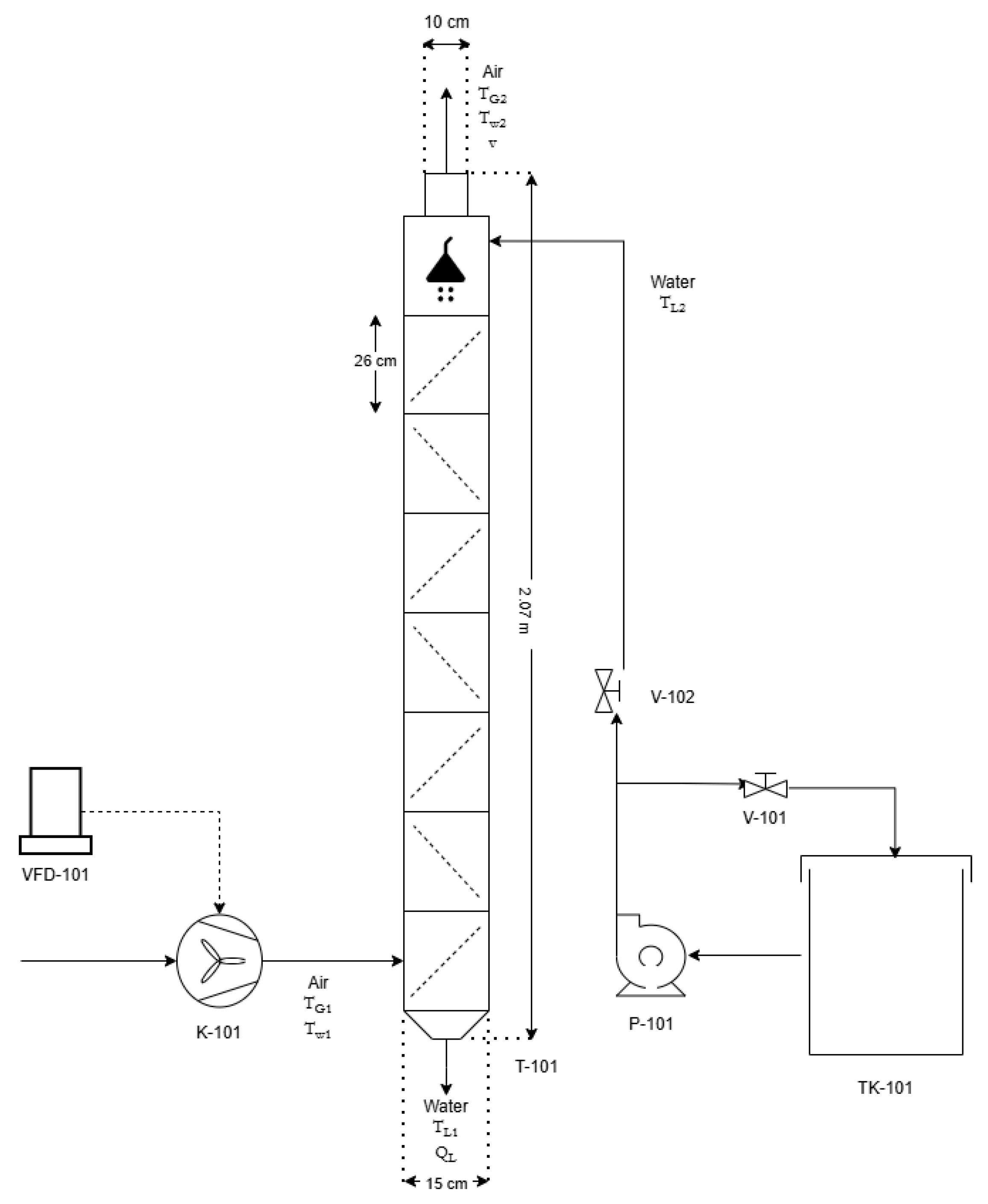
Figure 2.
Laboratory cooling tower system with perforated inclined plates and associated equipment.
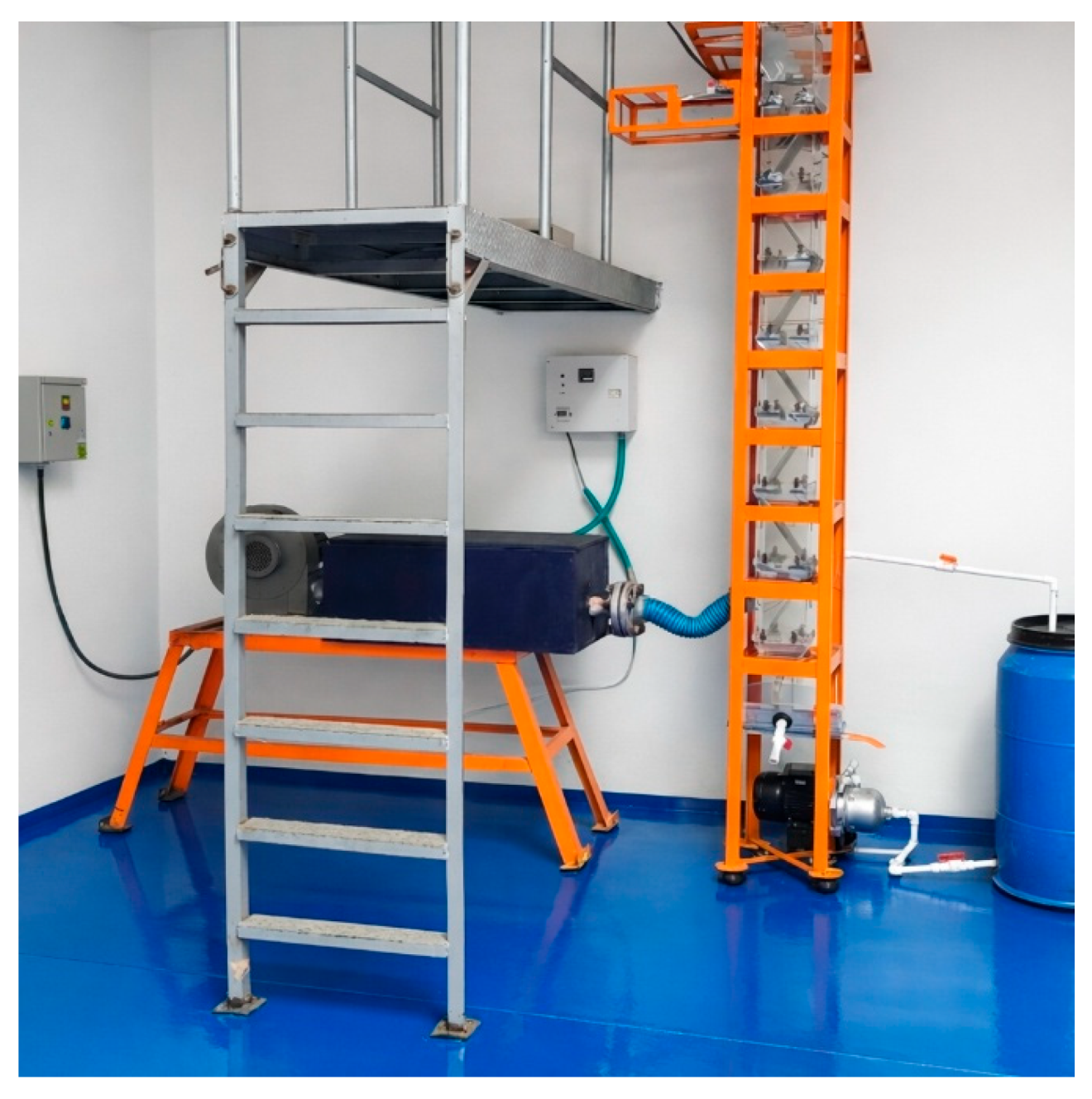
Figure 3.
Schematic representation of the 33-factorial design of experiment in the space of liquid mass flow rate L, gas mass flow rate G, and top water temperature TL2.
Figure 3.
Schematic representation of the 33-factorial design of experiment in the space of liquid mass flow rate L, gas mass flow rate G, and top water temperature TL2.
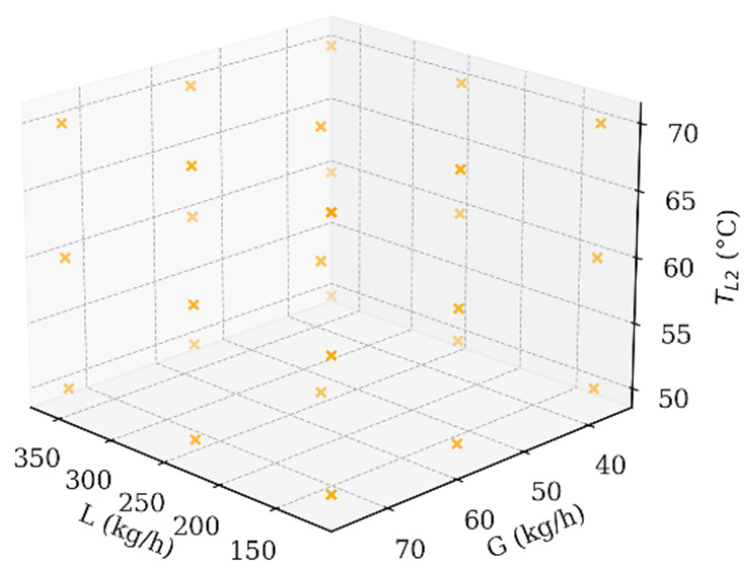
Figure 4.
Experimental volumetric mass transfer coefficient kya as a function of top water temperature TL2 for different gas flow rates at (a) L = 120 kg/h, (b) L = 240 kg/h, and (c) L = 360 kg/h.
Figure 4.
Experimental volumetric mass transfer coefficient kya as a function of top water temperature TL2 for different gas flow rates at (a) L = 120 kg/h, (b) L = 240 kg/h, and (c) L = 360 kg/h.
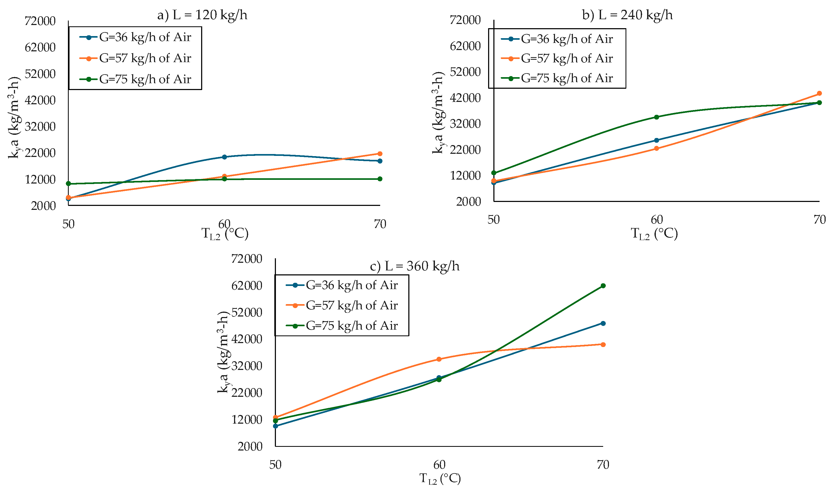
Figure 5.
Experimental volumetric mass transfer coefficient kya as a function of top water temperature TL2 for different liquid flow rates at (a) G = 36 kg/h, (b) G = 57 kg/h, and (c) G = 75 kg/h.
Figure 5.
Experimental volumetric mass transfer coefficient kya as a function of top water temperature TL2 for different liquid flow rates at (a) G = 36 kg/h, (b) G = 57 kg/h, and (c) G = 75 kg/h.
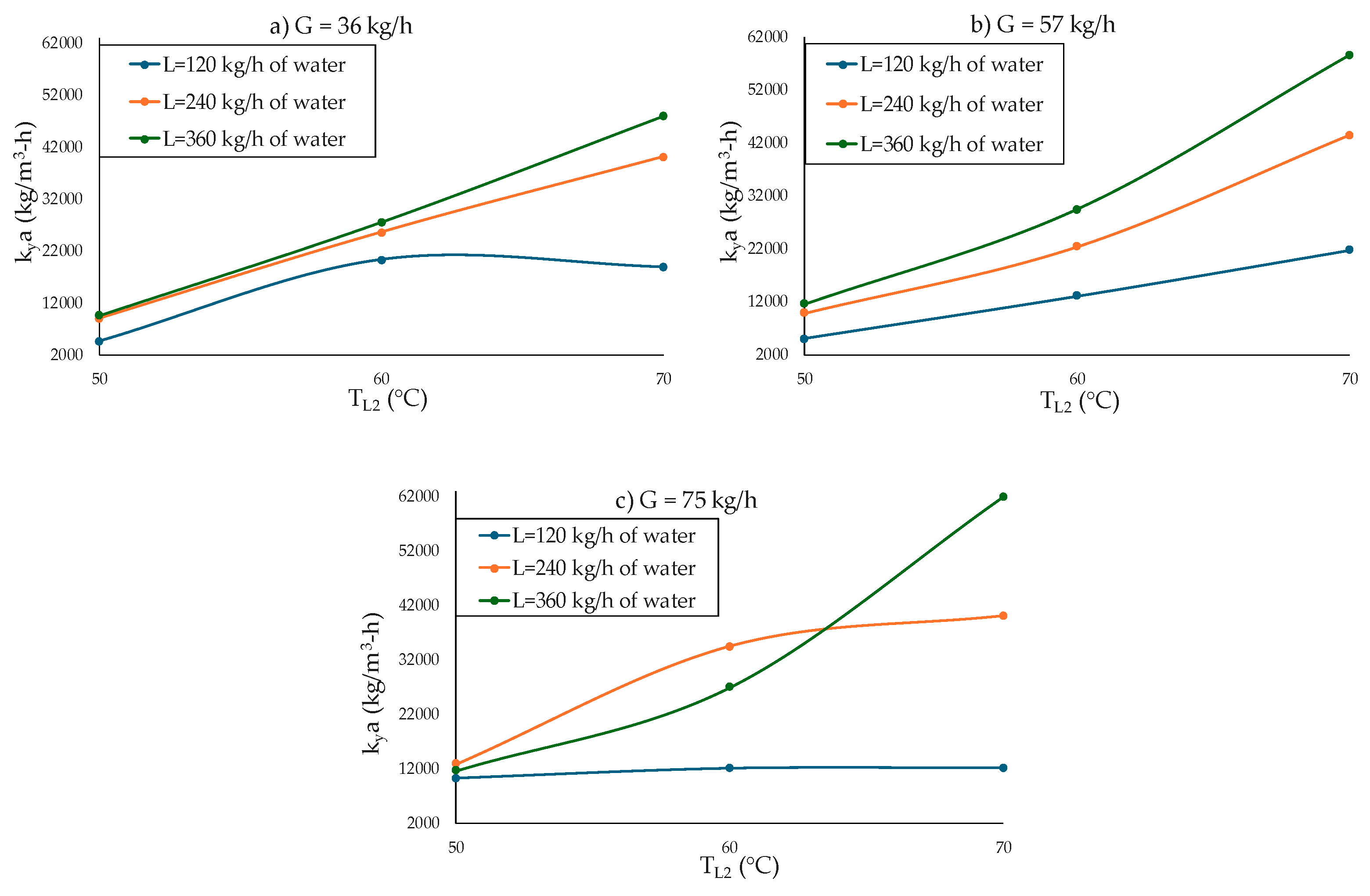
Figure 6.
Vertical temperature profiles of water and air along the column for G = 36 kg/h, and liquid mass flow rates (L = 120, 240, and 360 kg/h). Plots (a)–(c) correspond to TL2 = 50, 60 and 70 ◦C, respectively.
Figure 6.
Vertical temperature profiles of water and air along the column for G = 36 kg/h, and liquid mass flow rates (L = 120, 240, and 360 kg/h). Plots (a)–(c) correspond to TL2 = 50, 60 and 70 ◦C, respectively.
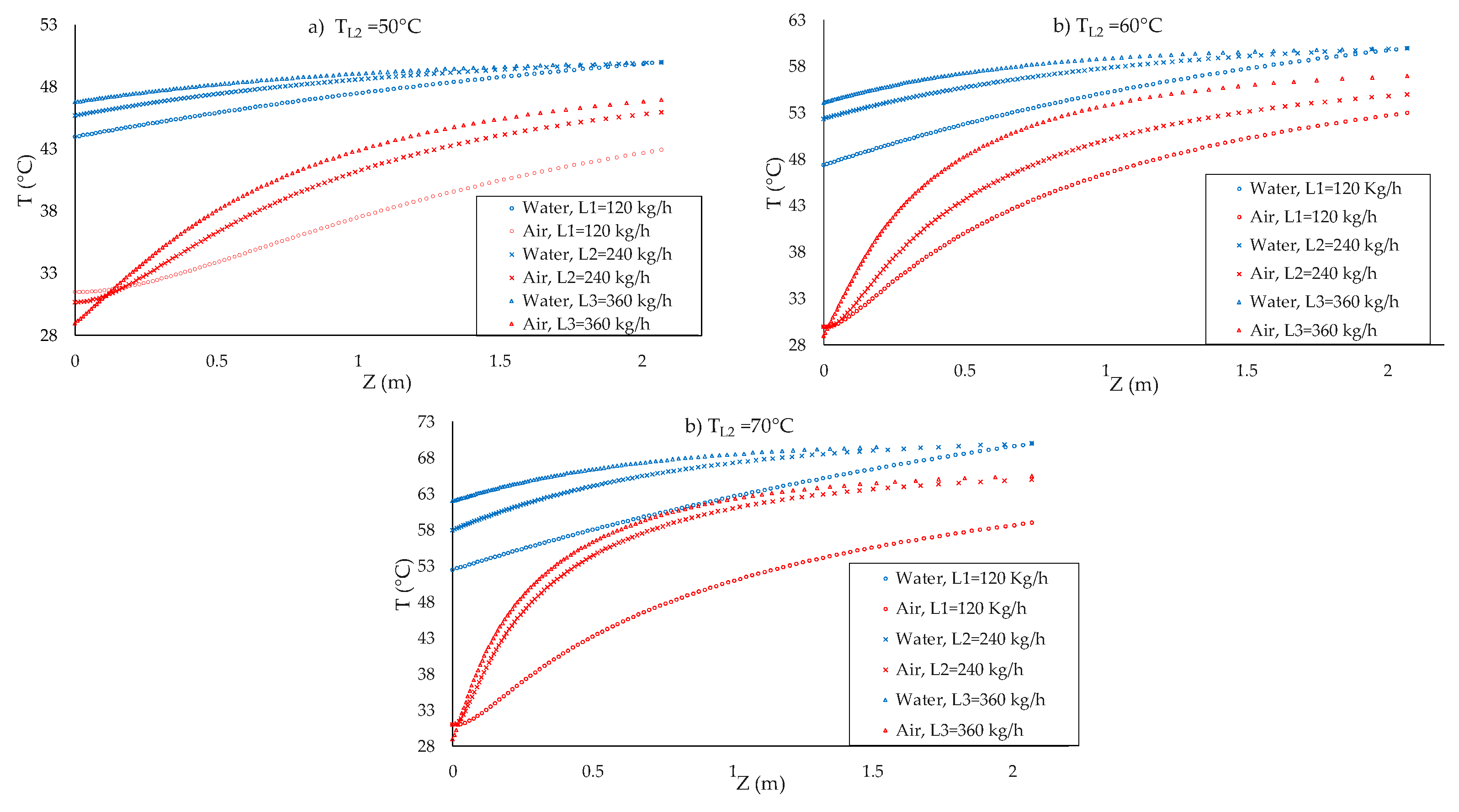
Figure 7.
Vertical temperature profiles of water and air along the column for G = 57 kg/h, and liquid mass flow rates (L = 120, 240, and 360 kg/h). Plots (a)–(c) correspond to TL2 = 50, 60 and 70 ◦C, respectively.
Figure 7.
Vertical temperature profiles of water and air along the column for G = 57 kg/h, and liquid mass flow rates (L = 120, 240, and 360 kg/h). Plots (a)–(c) correspond to TL2 = 50, 60 and 70 ◦C, respectively.
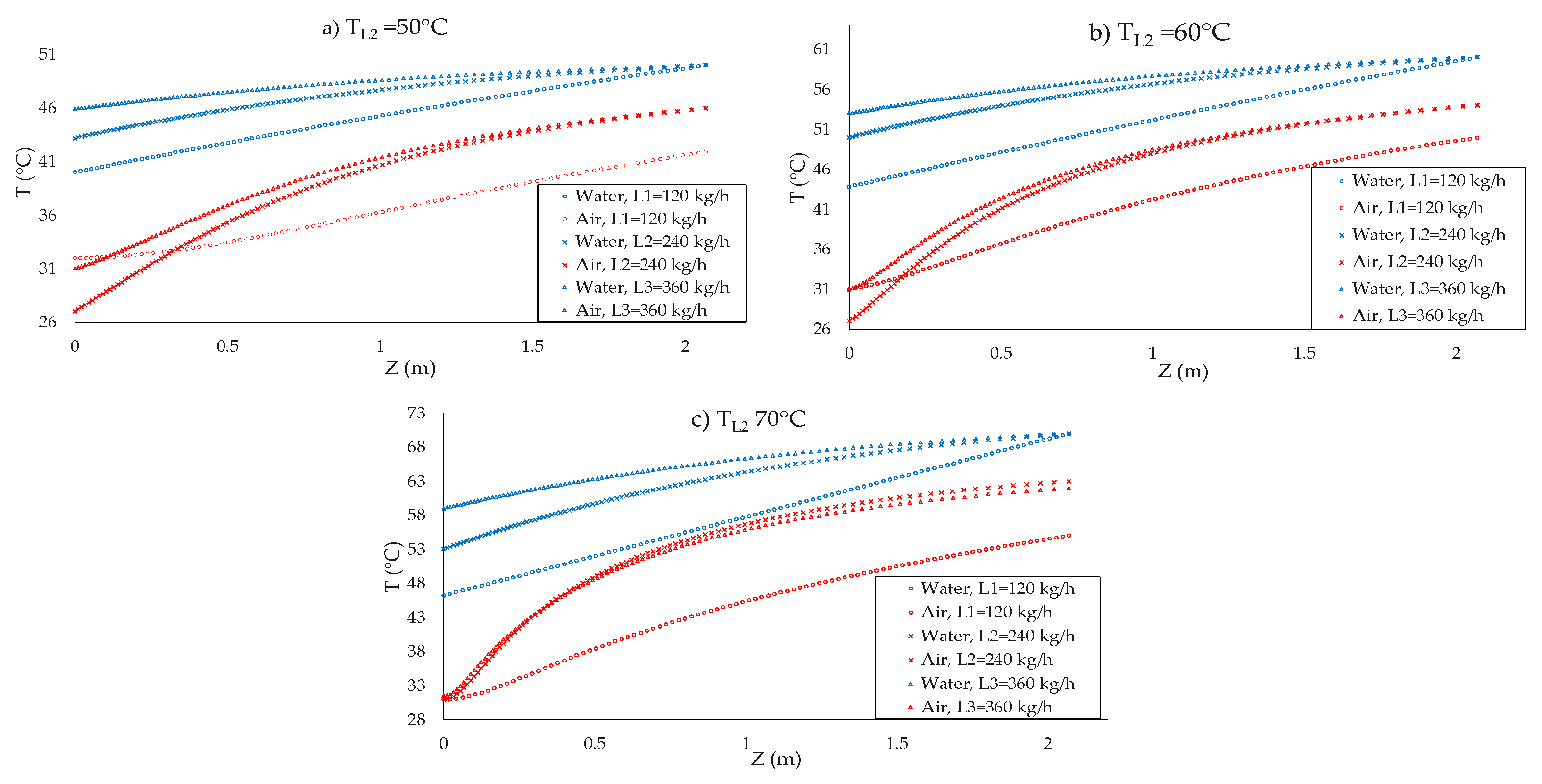
Figure 8.
Vertical temperature profiles of water and air along the column for G = 75 kg/h, and liquid mass flow rates (L = 120, 240, and 360 kg/h). Plots (a)–(c) correspond to TL2 = 50, 60 and 70 ◦C, respectively.
Figure 8.
Vertical temperature profiles of water and air along the column for G = 75 kg/h, and liquid mass flow rates (L = 120, 240, and 360 kg/h). Plots (a)–(c) correspond to TL2 = 50, 60 and 70 ◦C, respectively.
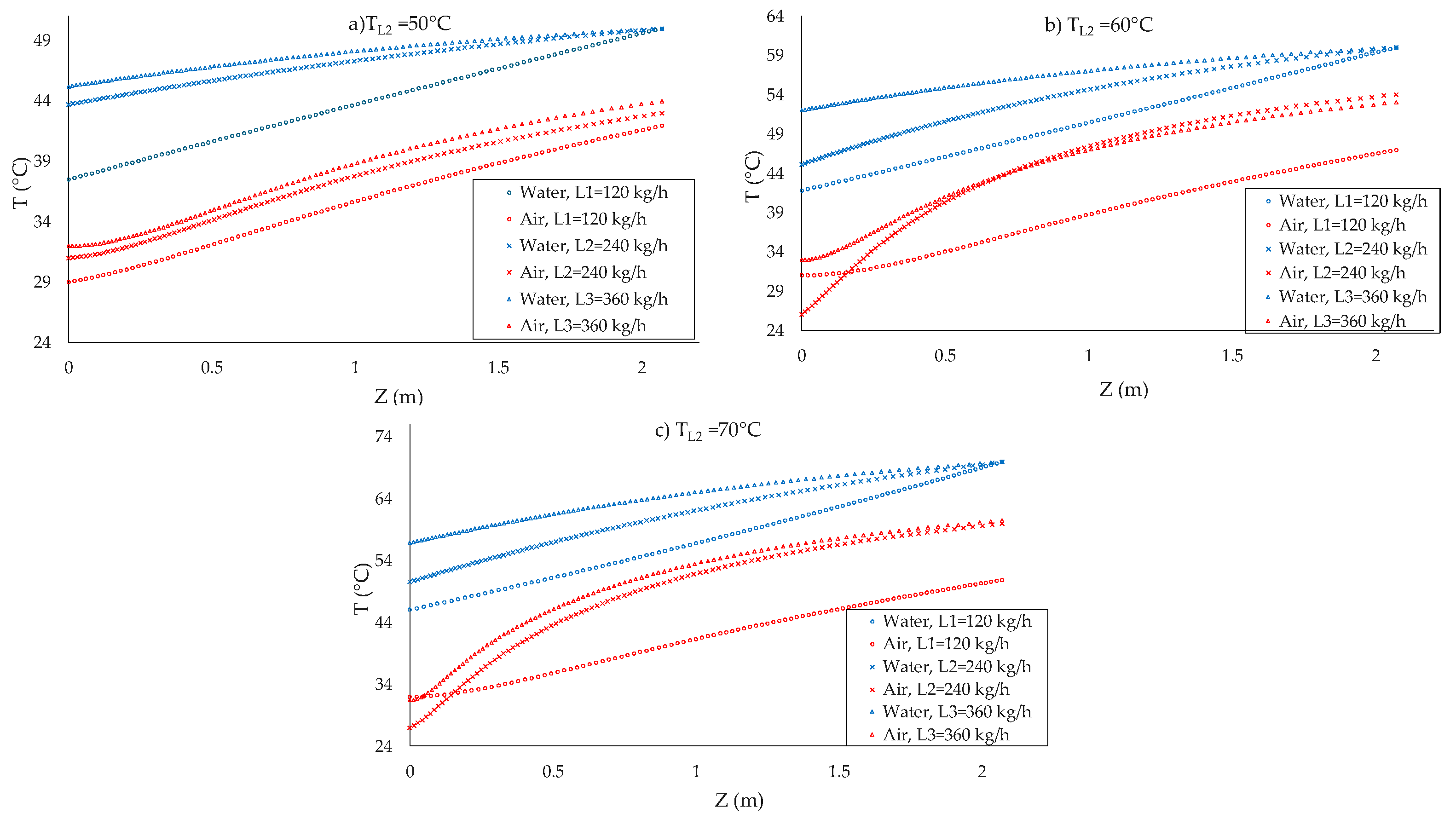
Figure 9.
Gas enthalpy profile as a function of the gas temperature (curved lines) and the water temperature (straight lines) for G=36 kg/h. Plots (a)–(c) correspond to liquid mass flow rates L=120, 240, and 360 kg/h, respectively.
Figure 9.
Gas enthalpy profile as a function of the gas temperature (curved lines) and the water temperature (straight lines) for G=36 kg/h. Plots (a)–(c) correspond to liquid mass flow rates L=120, 240, and 360 kg/h, respectively.
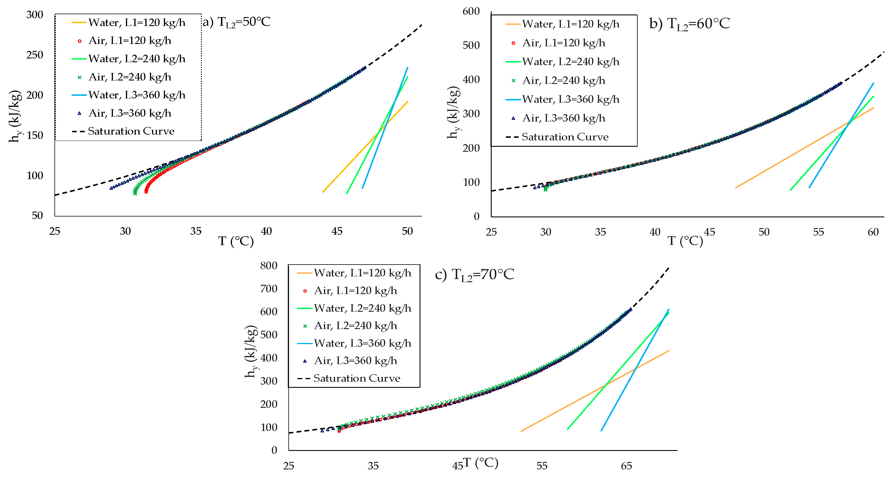
Figure 10.
Main effects plot for the volumetric mass transfer coefficient kya.
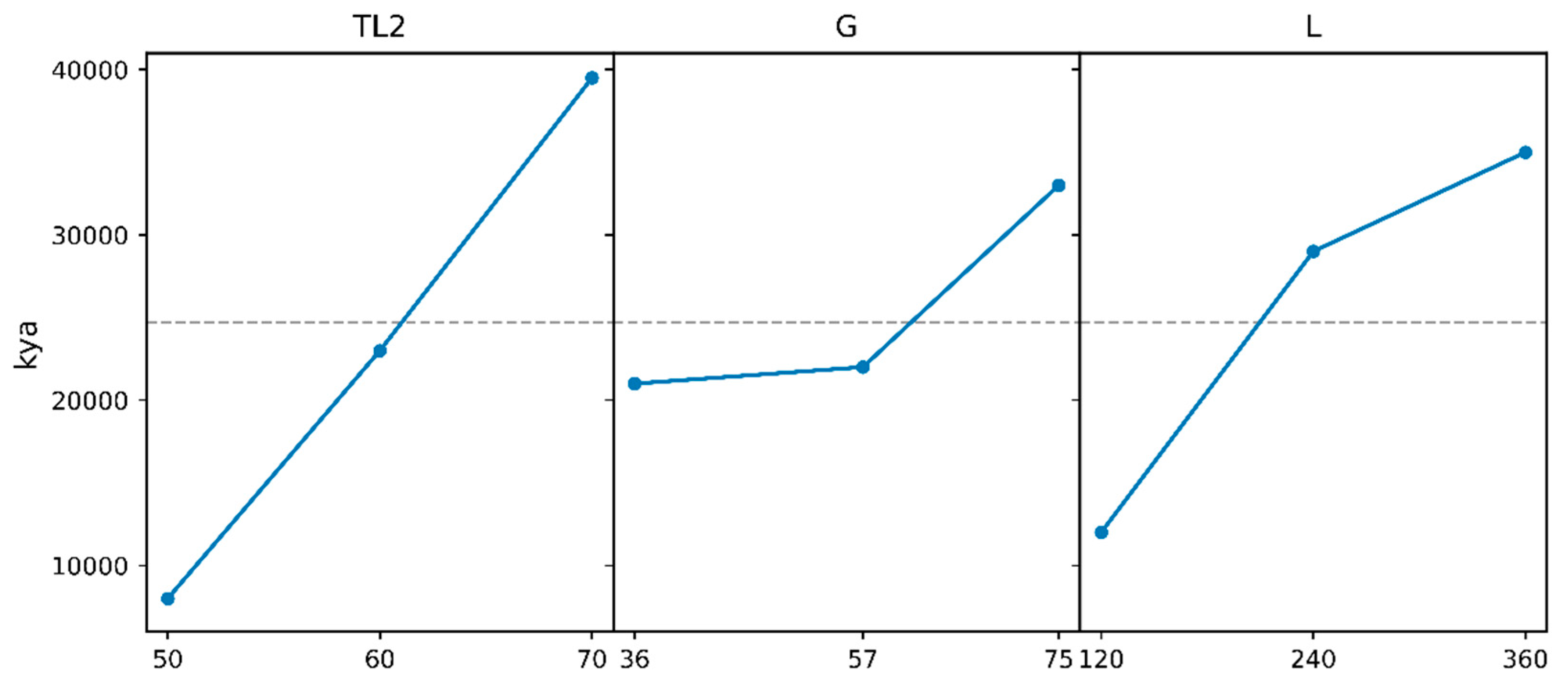
Figure 11.
Three-factor Interaction plot for the volumetric mass transfer coefficient kya.
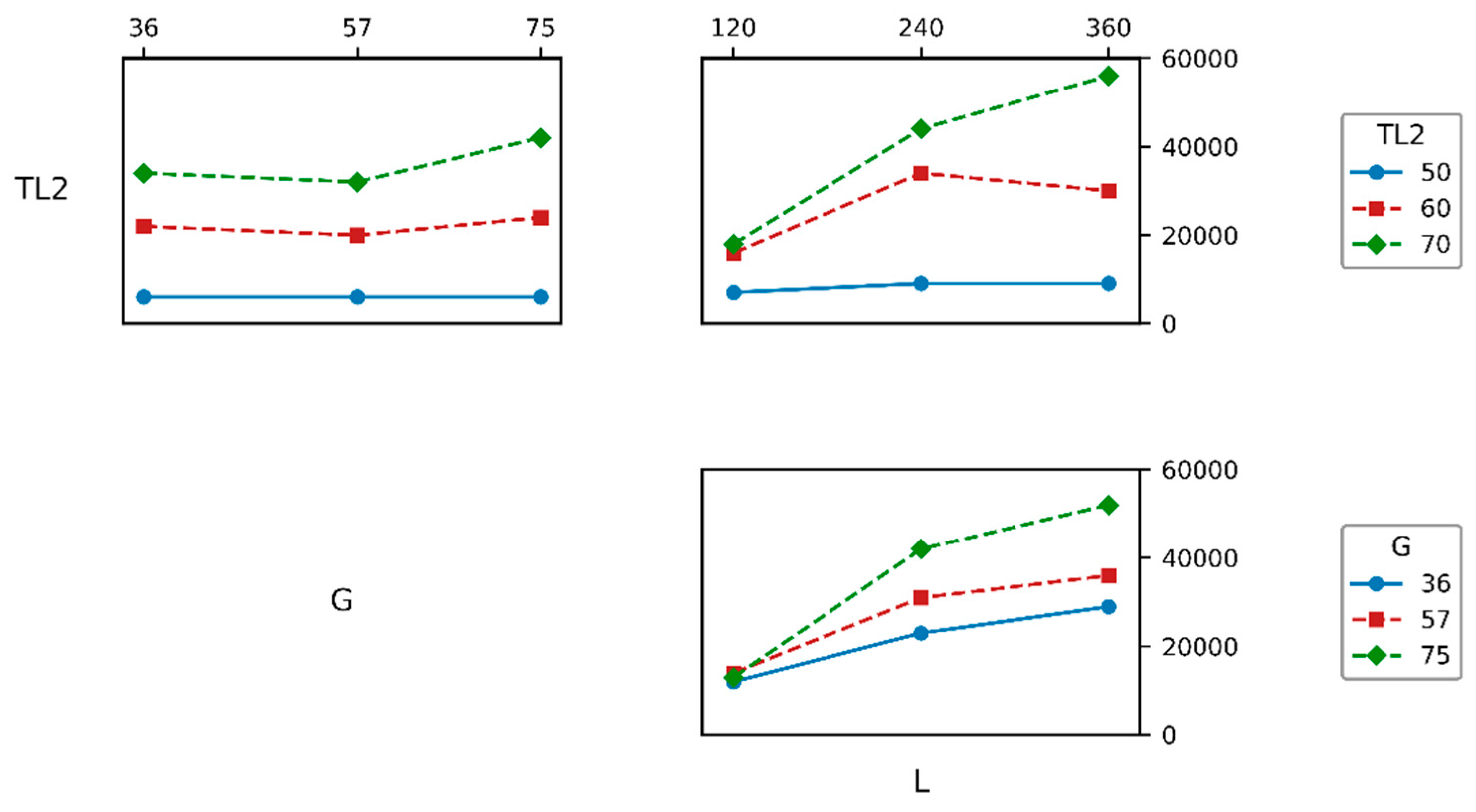
Figure 12.
Comparison of predicted and measured Outlet Water Temperature.
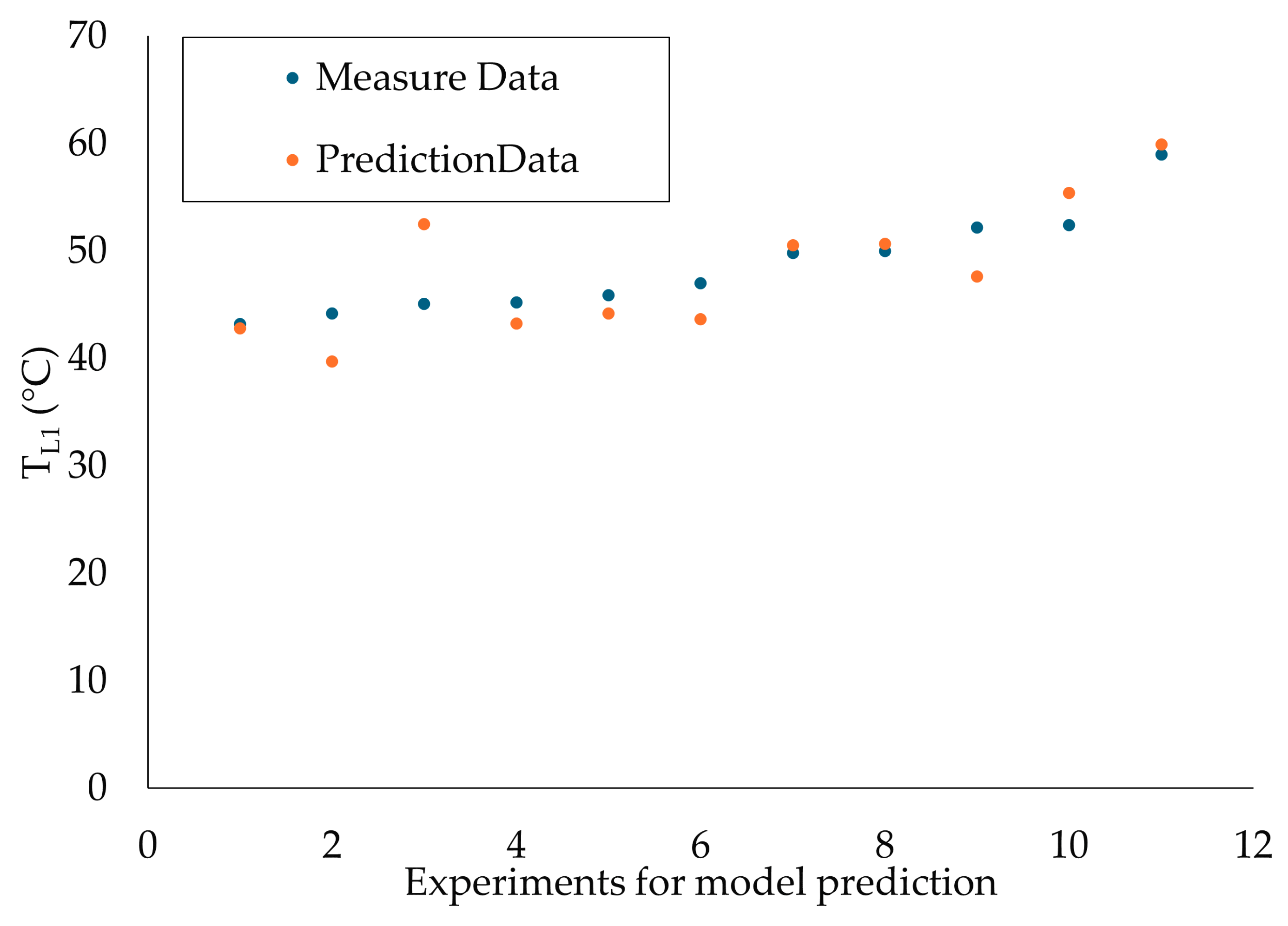
Figure 13.
Comparison of validated and measured Outlet Water Temperature.
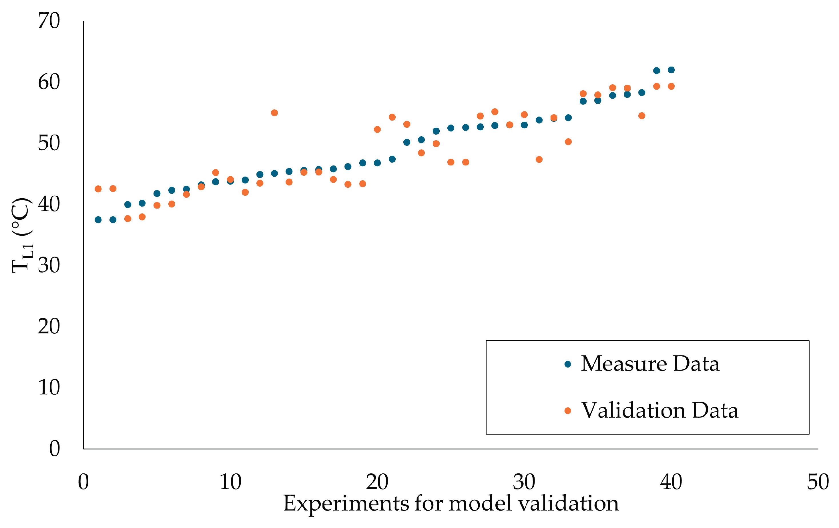

Table 1.
Factors and levels used in the design of experiments.
| Factor | Symbol | Level 1 (Low) | Level 2 (Medium) | Level 3 (High) |
|---|---|---|---|---|
| Liquid mass flow rate (kg/h) | L | 120 | 240 | 360 |
| Gas mass flow rate (kg/h) | G | 36 | 57 | 75 |
| Top water temperature (◦C) | TL2 | 50 | 60 | 70 |
Table 2.
Regression coefficients for the power-law correlation of the volumetric mass transfer coefficient.
Table 2.
Regression coefficients for the power-law correlation of the volumetric mass transfer coefficient.
| Model | ln K | α | β | γ |
| Proposed model (nominal G) | −11.93 | 4.173 | 0.149 | 0.756 |
Table 3.
Regression statistics for the proposed power-law correlation.
| Model | R2 | RMSE (kg/(m3·h)) |
Number of experiments |
|---|---|---|---|
| Proposed model (nominal G) | 0.869 | 5.93 × 10³ | 54 |
Table 4.
Analysis of variance (ANOVA) for the volumetric mass transfer coefficient kya.
| Source | DF | SS | MS | F | p-value |
|---|---|---|---|---|---|
| TL2 | 2 | 7175087629 | 3587543 815 | 52.11 | 0.000 |
| G | 2 | 91834930 | 45917465 | 0.67 | 0.518 |
| L | 2 | 3613427758 | 1806713879 | 26.24 | 0.000 |
| Error | 47 | 3235 831068 | 68847470 | – | – |
| Total | 53 | 14116181386 | – | – | – |
Table 4.
Regression statistics for the Outlet Water Temperature estimation.
| Key metric | Error |
| RMSEP | 10.70 |
| RMSECV | 4.54 |
Disclaimer/Publisher’s Note: The statements, opinions and data contained in all publications are solely those of the individual author(s) and contributor(s) and not of MDPI and/or the editor(s). MDPI and/or the editor(s) disclaim responsibility for any injury to people or property resulting from any ideas, methods, instructions or products referred to in the content. |
© 2026 by the authors. Licensee MDPI, Basel, Switzerland. This article is an open access article distributed under the terms and conditions of the Creative Commons Attribution (CC BY) license (http://creativecommons.org/licenses/by/4.0/).
Copyright: This open access article is published under a Creative Commons CC BY 4.0 license, which permit the free download, distribution, and reuse, provided that the author and preprint are cited in any reuse.


