
Submitted:
12 February 2026
Posted:
13 February 2026
You are already at the latest version
Abstract
Snow water equivalent (SWE), the amount of water that will be liberated when a given snowpack melts, is considered an essential climate variable. Snowmelt drives annual run-off in snow-dominant basins. However, detecting daily SWE changes in lake-effect snowfall regions such as the Great Lakes Basin (GLB), is challenging for classical methods. We developed a Siamese U-Net (Si-UNet) model to detect and characterize daily changes and trends in SWE. Our Si-UNet detected daily changes in SWE over the GLB with an F1-score of 98.73%. To characterize the basin-wide extent of anomalies in SWE distribution, we compared SWE trends to a 35-year median (35-YB) baseline and identified decadal trends in SWE. We found that the period from 1989 to 2008 was the temporal window with minimal anomalies, compared to the 35-YB of ~0.5108. Positive deviations from the 35-YB were prevalent over these 20 years, indicating less significant daily changes. A significant shift to daily SWE similarity below the 35-YB occurred after 2009, especially in January and February. Daily changes in SWE were high in April, beginning in the second week. The strongest positive trend, likely associated with lake-effect snowfall, was observed in April 2000 (R2 = 0.47).
Keywords:
snow water equivalent
; Great Lakes
; daily snow change
; snow trend anomaly
; Siamese network
; climate change
1. Introduction
The Great Lakes Basin (GLB) is one of the most populated watersheds in North America, with an estimated population of approximately 40 million people. About 63% and 37% of the population live in the U.S. and Canada, respectively [1]. Snow is crucial for sustaining the ecosystems and human communities’ overall well-being in the GLB [2]. Snow covers a pronounced proportion of the Canadian landmass during winter [3], and produces water that recharges groundwater resources, freshwater ecosystems, and contributes to irrigation [4,5].
Snowfall modulates lake ice levels by forming thicker snowpacks [6,7]. Lakes without seasonal ice cover experience high air temperatures [8]. Snow cover also influences soil temperature, soil freezing and thawing processes, and permafrost formation, with a profound impact on carbon and hydrological cycles, especially in the cold regions [9,10]. The timing, duration, accumulation, and melting processes of seasonal snow cover dictate its impacts on the Earth’s thermal regime [9]. The rate and timing of snowmelt affect runoff, which in turn influences plant-available water storage [11]. Rapid fluctuations in snow depth during the winter influence soil temperature and moisture, leading to varying patterns of soil respiration [12]. Increased snowmelt may result in soil attaining field capacity rapidly, stimulating below-root zone percolation and streamflow, whereas slower snowmelt may decrease streamflow [13,14]. For example, using hydrological model simulations and a new snowmelt tracking algorithm, it was shown that although 37% of precipitation falls as snow, 53% of the total runoff in the western United States emanates from snowmelt [15].
The winter climate over North America, driven by both climate-induced events and natural atmospheric cycles (e.g., Pacific Decadal Oscillation and El Niño Southern Oscillation), is changing in unpredictable ways [16]. Diverse variables, including temperature, precipitation, and the snow-albedo feedback, influence snow cover [17,18,19,20,21]. However, climate-induced variables portend the most detrimental effects, causing a shift in storm tracks with predictable consequences on the snow regime [22]. Climate warming is projected to exacerbate changes in snow parameters, snow onset and retreat periods, with unpredictable impacts on the Great Lakes water levels and the viability of its ecosystems [23]. The Great Lakes region experiences local precipitation bands, elevated convection, and lake effect snow bands, which enhance snowfall events [24]. Despite the prevalence of lake-effect snowfall (LES), under high greenhouse gas emission scenarios, snow water equivalent (SWE) is projected to decline in the snowbelt regions to the lee of Lakes Erie and Ontario [25].
Rapid snowmelt, driven by factors such as rain-on-snow, reduces the formation of snowpacks and increases the risk of flooding [26]. Thus, detecting changes in snow parameters is an important piece of information for managing water resources as well as planning and adapting to climate change impacts, yet the relationship between seasonal snow and climate variables is uncertain and non-linear, complicating SWE trend analysis [27]. Additionally, detecting and attributing changes in snow over the GLB is not a straightforward task due to the spatially heterogeneous nature of snow ablation processes [28]. Kunkel et al. [29] further emphasized that non-climatic issues complicate the identification of significant change and trends in snow variables. Therefore, methods that are invariant to stochastic internal variability and seasonal patterns of snow spatial structure are crucial for obtaining accurate estimates of changes in snow parameters.
Under climate change, large-scale losses of snow are projected, raising considerable concerns over future freshwater resources, especially in snow-dominated watersheds, where snowmelt has profound effects on streamflow dynamics [19,30,31]. Therefore, it is imperative to unravel how snow processes have transformed over recent decades and to do so at very high temporal resolutions to inform water resources planning, management, and adaptation to natural hazards such as snowmelt-induced floods. The overarching objectives of this study are to: (a) demonstrate Siamese UNet’s capability to detect basin-scale changes in snow parameters, (b) estimate daily changes in SWE at the watershed scale, and (c) characterize decadal trends and anomalies in SWE distribution over the GLB.
1.1. Snowfall Dynamics in the Great Lakes Basin
Synoptic-scale analysis provides evidence that the Great Lakes exert a strong influence on the patterns of snow accumulation and ablation (i.e., Lake-induced snowfall) [32,33,34]. Although Lake-effect snowfall is known to drive an increase in the snowfall/snow water equivalence ratio in the GLB, time series analysis of snowfall within lake-effect areas shows that this pattern likely began in the 1930s and ended in the early 1970s [35]. Lake-effect snowfall is found to increase snowfall in most regions of the Great Lakes. For instance, elevated lake-effect snowfall near the Great Lakes from 1951 to 1980 [36]. In a related study, Burnette et al. [37] identified persistent upward snowfall trends in the lake-effect snowbelt areas of the Great Lakes region until the end of the century. Ellis and Johnson [35] also identified a 40-year upward trend in snowfall from 1930 to 1970, followed by less significant trends after this period.
Contrary to these trends, meteorological variables and weather types are becoming more favourable for snow ablation in the GLB; these include elevated air temperatures, southerly wind flows, less cloud cover, and increased liquid precipitation rates during the winter months [38]. Consequently, several studies have reported declining snowfall events in the GLB. For example, seasonal basin-wide snow depth was found to have declined by approximately 25% from 1960 to 2009, especially in the northern part of Lake Superior [39]. In a related study, analysis of snowfall and total precipitation trends over the Great Lakes from 1980 to 2015 revealed a significant decrease in snowfall at a rate of 40 cm/36 years, along the Ontario snowbelts of Lake Superior and Lake Huron-Georgian Bay [40].
Kunkel et al. presented a 107-year analysis of snow trends over the conterminous United States and found that from 1950 to 2006, snow trends in the central and northwest U.S. regions experienced significant declines in high-extreme snowfall years, while four regions (i.e., Northeast, Southeast, South, and Northwest) showed significant increases in the frequency of low-extreme snowfalls [41]. Snowfall and total precipitation trends were derived for the GLB from 1980 to 2015, revealing a significant decrease in snowfall, at a rate equivalent to 40 cm/36 years, and a considerable reduction of total precipitation of 20 mm/36 years, especially in Lake Superior and Lake Huron-Georgian Bay along the Ontario snowbelts [42]. Furthermore, extreme daily snowfalls have been found shift northward, with large daily changes occurring along the US-Canada border [43]. These findings are corroborated by snow projections in Central and Eastern North America, affirming a decline in extreme snowstorms southward, while the northern regions experience increased snow water equivalent and frequency of snowstorms [44]. In addition, declines in mean annual SWE, high-frequency of low-snowfall years, and less frequent high-snowfall years were projected for the western United States [45]. Furthermore, in western North America, annual snow water storage was reported to have decreased from 1950–2013 as a consequence of early snowmelt, rainfall in spring months, and decreases in winter precipitation [46].
Despite these consistent findings, Kunkel et al. [29] point out temporal inconsistency and inhomogeneity in the data employed to conduct most of these analyses and call for the use of more homogeneous datasets. For instance, using a set of consistent station data, an upward trend in snowfall was identified in Superior and Michigan, largely attributable to warmer surface water and less ice cover [33]. This suggests that gridded snow data hold the potential for a more enhanced and spatial-temporally continuous representation for studying snow. For example, the Snow Data Assimilation System SWE was employed to model snow processes for climate-related water resources studies in the Great Lakes watersheds [47] and stream flow in eastern Canadian basins [48].
2. Materials and Methods
2.1. Study Area and Data
Our study area covers the five Great Lakes and their watersheds. Using ArcGIS Pro’s ArcPy Package, the GlobSnow SWE data was clipped to a spatial extent encompassing 72 × 72 pixels. The GlobSnow’s SWE has a spatial resolution of 25 km × 25 km, covering an area of 1,800 km2, given the spatial extent of 72 × 72 km. This area encapsulates the GLB and its surrounding ecosystems. We reprojected the data, adopting an Equal Area Projection (e.g., Lambert Equal Area Projection) to maintain the original grid area. Figure 1 depicts the SWE distribution in early, mid, and late February and March over the GLB in 2020. The northwestern part of the GLB, corresponding to the Lake Superior basin, can be seen to have relatively elevated levels of SWE in February. A northward shift in SWE can be observed between February and March. This gradual transition is indicative of the end of the Winter season in the GLB.
2.2. Training Sample Processing and Labeling
We labeled the training data following the methods illustrated in Malik and Colin [49]. Thus, SWE samples at one day interval were labeled as positive (No Change), whereas SWE observations that were two or more days apart were labeled as Change instances. We deployed a spatially-explicit metric – the Structural Similarity (SSIM) index to inspect and exclude ambiguous training examples using 0.98 and 0.90 as thresholds for positive pairs (No Change instances of SWE) and negative pairs (Change instances of SWE), respectively, as shown in [49]. For model development, we used data from 1979 to 2001. The training and validation data splits were 75% (training set) and 25% (validation set). Independent validation consists of data from 2002 to 2018. We separated the data into seasons or months and evaluated the model’s performance across seasons.
2.3. Siamese U-Net Architecture and Training
Our model architecture, with the SSIM index combination, is simplified and depicted in Figure 2. The model receives 72 × 72 GlobSnow SWE data and outputs the same spatial extent at the decoder branch. Using the SSIM index, the resulting outputs from the two-sister decoders are compared, focusing more on changes in the spatial structure SWE. The computed similarity value is passed to a loss function for error estimation and optimization during model training. An exhaustive description of this learning paradigm is outlined in [49,50]. The Model is trained using Keras-Tensorflow framework with NVIDIA GPU memory of 40 GB. Fifty epochs were used with Early Stopping and a patience parameter of 10. Drop-out, batch-normalization, and ReLU activation function were applied.
2.4. Model Accuracy Metrics
To assess the model’s accuracy on the prediction of No Change versus Change instance of SWE, we adopted the metrics: true positive rate (TPR), true negative rate (TNR), false positive rate (FPR), false negative rate (FNR), Precision (PR), F1 score, and overall accuracy (OA) to assess the models’ prediction of SWE similarity and change.
TPR measures the proportion of SWE samples that are correctly predicted as No Change instances; TNR, on the other hand, estimates the fraction of SWE samples that are accurately detected to be Change instances. Thus, FPR = 1 –TNR, and FNR = 1 – TPR. Equations 1 – 5 represent the accuracy metrics. Area Under the Curve of the Receiver Operating Characteristics (AUC-ROC) was also derived to examine TPR and FPR over a range of thresholds.
2.5. Deriving the Daily Snow Water Equivalent Similarity Vector
To estimate daily SWE change events, the pre-trained Si-UNet, after rigorous accuracy assessments, can be employed to make predictions over a series of SWE observations, generating a time-series vector consisting of similarity values between consecutive days. High similarity values are indicative of less pronounced changes; contrarily, low similarity values characterize profound changes in SWE. We formulate the solution as illustrated in [49,50]. The SWEsim vector, which represents daily SWE similarity, is derived using the equation 6 to accumulate the daily SWE similarity values.
Where t and m represent day and month, respectively. Accordingly, denotes SWE sampled on the ith day. The model term in the equation denotes the Si-UNet.
Using the SWEsim vector, we derived long-term median SWEsim from 1981 to 2016 to compare deviations in SWE over 35 years (Equations 7 and 8). We refer to this median as a 35-year baseline (35YB). Deviations from 35YB will be indicative of anomalous SWE trends at basin scales.
3. Results
3.1. Model Accuracy Assessment Report
Figure 3A presents a range of possible thresholds for the model’s predictions of SWE similarity, while the AUC-ROC is depicted in Figure 3B. The F1-score, Precision, and Recall appeared to be constant as the threshold parameter was varied until 0.45, where it began to rise steeply. All the accuracy metrics reached the optimum value at a 0.5 threshold. The F1-score and Recall dropped to 0 when the threshold exceeded 0.5. Contrarily, the false positive predictions reduce to near zero, resulting in Precision scores rising to 1.0 after a 0.5 threshold. The AUC-ROC started at 0.8, increasing gradually to 1.0, and stabilized at this point throughout the range of possible thresholds. These thresholds are values that were greater than or equal to 0.5.
We compared the accuracy of our proposed Si-UNet to the CNN baseline, using the SSIM index and Euclidean Distance (ECD) metric. Further, we investigated the performance of the models given a choice of loss functions – binary cross-entropy loss (BCE) and contrastive loss (CL). Table 1 presents a summary of the models’ accuracy. It can be observed that our model, with the CL and SSIM index, though has a narrow threshold value (i.e., 50%), tends to outcompete the other models, yielding an F1-score of 98.73%. The most challenging instances were the change-pairs (i.e., negative labels), resulting in a TNR of 92.82%. Surprisingly, the base CNN with ECD can be observed to excel at detecting instances of SWE change (TNR) with 99.44% accuracy; the model’s performance at detecting the No Change (TPR) instances tended to be the worst (92.84%), however.
3.2. Empirical Evaluation of Snowfall and Ablation in the Great Lakes Basin
Our model identified three types of sequential snow-related events that create daily variation of SWE trends in the GLB. The first is an alternating increase in snowfall (i.e., snow accumulation) and decreases in snow on the ground (i.e., snow ablation). We termed this sequence a snowfall-ablation (SA) event. This yielded upward- and downward-pointing peaks that characterize sharp transitions between snowfall and ablation events. For example, on the graph in Figure 4, points 2, 11, and 25, corresponding to SWEsim values: 0.523, 0.525, 0.526, represent days with pronounced snowfall, whereas points 7, 9, and 12, aligning with SWEsim: 0.515, 0.516, 0.520, were days that experienced snow ablation. Upward peaks are associated with high SWE similarity, while downward peaks signify low SWE similarity. The second sequence type is snowfall-snowfall (SS), and the third, ablation-ablation (AA). The SS is characterized by two or more consecutive days of snowfall, resulting in pronounced snow accumulation that increases snow depth and, predictably, the amount of SWE (Figure 4, D, E, F). Conversely, AA events are 2 or more consecutive days of snow ablation; hence, resulting in a substantial SWE reduction (Figure 4, A, B, C). Both SS and AA events induce ridges or crests and troughs in daily SWE trends. However, crests are largely generated by SS events in snowfall-dominant months (e.g., January, February, and March), whereas AA events frequently induce troughs. Figure 4 depicts the three types of events, with arrows showing the monotonic pattern and direction of change. The most perceptible pattern (shown in the red rectangles) is SA events in the eastern wing of the Lake Michigan sub-basin. Also noticeable is the SS event in the northwestern part of Lake Ontario sub-basin (shown in the green rectangles). The dashed lines represent simple linear regression (orange) and the 35YB (black). The computed 35YB is ~ 0.5108, aligning closely with the No Change SWE instance (i.e., No Change SWE days for the Si-UNet model prediction). Thus, it can be observed that all the SWEsim values for February 1990 were above the reference 35YB.
3.3. Great Lakes Basin Daily SWE Trends
Using the vector, we present 30-year daily SWE similarity trends from 1989 to 2018 (Figure 5, Figure 6 and Figure 7). The y-axis and x-axis represent SWE deviations from 35YB and days, respectively. The blue trend lines denote daily variability in SWE, and the red lines are linear regression conditioned on . Positive (i.e., positive SWE anomaly) and negative (i.e., negative SWE anomaly) deviations are values above and below the 35YB, respectively. Zero values, on the other hand, signify no deviation from the 35YB. Positive and negative deviations are largely associated with high and low SWE scenarios, respectively. Both deviation types are a function of snowfall and SWE reduction induced by ablation events.
In April (Figure 5), strong statistically significant increases in SWE similarity were detected in 1991 and 1993 (R2 = 0.28 and 0.3, respectively). Contrarily, 1989, 1992, 1996, and 1997 all exhibited a significant decline in SWE similarity (R2 ranged from 0.22 – 0.46). In March, less substantial increases and decreases in SWE trends dominated. It can be observed that the declining trends occurred when the SWE similarity decreased in mid-March (e.g., 13–17 March). These trends are more obvious in March 1990 and 1995. Two statistically significant but opposing trends were observed in February 1994 and 1995. While SWE declined significantly in 1994 (R2 = 0.39), it increased significantly in 1995 (R2 = 0.57). January and February depicted a predominantly increasing SWE similarity and trend. While the SWE trends in 1996 and 1997 were not statistically significant, the trends for most years were characterized by substantial positive SWE trends. One notable exception was February 1994, in which the trend was significantly declining (R2 = 0.39).
Figure 6 shows daily changes in SWE from 1999 to 2008. Significant positive SWE trends can be observed in April, with R2 ranging between 0.41 – 0.72. The strongest positive trends were observed in 2000 (R2 = 0.47) and 2005 (R2 = 0.72). The 2000 trend was driven largely by snow accumulation (i.e., SS events) occurring after April 5th, whereas the 2005 trend can be attributed to AA events starting on April 5th and progressing gradually until the end of April. A moderately strong negative trend was observed in 2002 (R2 = 0.21). SWE trends in March were predominantly weakly positive. The most significant positive trend was observed in 2000 (R2 = 0.32). February and January were characterized by positively significant trends in SWE. February 1999 and 2005 recorded high SWEsim values with strong positive trends (R2 = 0.3 and 0.60, respectively), whereas January 2001, 2003, and 2008 portrayed competing positive trends (R2 = 0.43 – 0.44).
Daily changes in the GLB SWE are depicted in Figure 7. A predominant negative trend characterized the SWE pattern from April 2008 to 2018. While a significant positive SWE trend was observed in 2010 (R2 = 0.39), the remaining years exhibited negative SWE trends (R2 = 0.2-0.59). The decline frequently occurred between April 13th and 17th for most of the years. March was characterized by frequent positive trends, with highly significant SWE increase occurring in 2014 and 2015 (R2 = 0.37 and 0.27, respectively). Contrary to March trends, February and January depicted a substantial prevalence of non-significant trends. In February 2009, 2016, and 2017, SWE exhibited increasing trends (R2 = 0.22, 0.20, and 0.36, respectively), while the rest of the years showed no statistically significant change. For example, January largely portrayed no significant trends, and where trends were observed (e.g., 2010 and 2018), they tended to be weakly significant.
3.4. SWE Anomaly Frequency in the Great Lakes Basin
The frequency of SWE deviation (in days) from the 35-YB throughout January, February, March, and April (JFMA) is depicted in Figure 8, Figure 9 and Figure 10. The y-axis denotes the frequency of days having values above or below the median, whereas the x-axis represents deviation from the 35-YB. The red dotted vertical line demarcates deviations below and above the median (i.e., values below and above zero).
Figure 8 depicts SWE deviations from the 35YB SWEsim between 1989 and 1998, through JFMA. The histogram bins are more clustered and continuous for most of the months and years. Aside from January 1994 and 1995, when SWE was largely below the baseline, the rest of the years had either high SWEsim values or a balanced frequency above and below the baseline. Contrary to this trend, from February 1989 to 1998, SWE exhibited consistently higher and clustered SWEsim values. The deviations were between -0.005 and +0.01 with frequencies starting at ~2 days. SWE anomaly patterns in March also align with February, as positive deviations (i.e., SWEsim values above the 35-YB) were prevalent. The deviations for February, March, and April exhibited balanced frequency from 1993 to 1995. Similarly, April was characterized by symmetrical frequency of values below and above the baseline. The only notable exceptions were 1990 and 1996. These years incurred two contrasting SWE deviations: pronounced daily changes in SWE, resulting in high frequencies of deviations below the 35YB (April 1990), and fewer daily changes, yielding high frequencies of deviations above the 35YB (April 1996).
From 1999 to 2008 (Figure 9), it can be observed that January exhibited the lowest SWE similarity values (i.e., values below 0.5108), while there was a balance between daily occurrences of low and high values in April. Contrarily, the frequency of daily occurrences of high SWEsim values appeared to be elevated in February and March. A notable exception was in 2007, wherein JFMA exhibited values below the 35YB, with deviations ranging from -0.01 to -0.03.
Figure 10 presents SWE deviations between 2009 and 2018 compared to the 35-YB. It can be deduced that January and February tended to have anomalously low SWEsim values, ranging from -0.01 to -0.05. Except for 2009 and 2018, where higher SWEsim values were recorded in March, the remaining years elicit a balanced frequency of daily variability in SWE. Similarly, April 2010, 2012,2013, and 2014 were characterized by balanced frequencies of daily changes in SWE relative to the 35-YB.
4. Discussion
In this study, we developed a U-Net model inspired by the Siamese model architecture for detecting anomalies in classification tasks [51]. Our model detected daily changes in SWE with 98.73% accuracy (F1-score), outcompeting the baseline CNN and U-Net models without spatially-explicit metrics (i.e., the SSIM index). The AUC-ROC of 0.997 further accentuates the model’s robustness in detecting changes in SWE. Guided by the SSIM index, the model evaluates SWE similarity based on structural differences between pairs of consecutive SWE samples. This reduces the models’ tendency to capture spurious structural differences that are not related to the underlying spatial processes driving snow accumulation and ablation [52,53].
We computed a 35-year median baseline SWE similarity (i.e., 35YB) of ~ 0.5108 and identified three types of alternating snow-related events using a sample SWE times series in February, which is the SWE month dominant month in the GLB: (1) is snowfall-snowfall (SS), (2) ablation-ablation (AA), and (3) snowfall-ablation (SA). These events characterize transitions between snowfall and ablation processes (Figure 4). The points 2, 11, and 25, in Figure 4, correspond to SWEsim values: 0.523, 0.525, and 0.526. These were days with pronounced snowfall. Conversely, in Figure 4, points 7, 9, and 12 were days experiencing high ablation. Thus, the SWEsim values tended to be relatively low, 0.515, 0.516, 0.520, respectively. The most perceptible pattern is SA events in the eastern wing of the Lake Michigan watershed. Also noticeable is the SS event in the northwestern part of Lake Ontario (Figure 4). While the northern and southern parts of the GLB, respectively, experience peak ablation events in April and February, most of the regions in the basin experience peak ablation in March [54]. This pattern may have an impact on March SWE anomalies by increasing the frequency of days incurring SWEsim below the baseline. Ablation events have been found to decrease within the northeastern and northwestern Lake Superior basins, while occurring frequently in the eastern Lake Huron and Georgian Bay basins [54]. This pattern is obvious in Figure 4, where SWE persists around the Lake Superior sub-basin throughout February.
Alternating positive and negative deviations are signs of snowfall-ablation, which creates sharp peaks in the time series (i.e., trend line). The trend line becomes virtually flat (e.g., R2 < 0.001), with less pronounced crest and trough regions when the magnitude and frequency of alternating snowfall and ablation events are equivalent (e.g., Figure 5, February 1989). Figure 5, Figure 6 and Figure 7 present 35-year daily SWE trends over the GLB. Linear regression conditioned on the days of SS, AA, and AS revealed complex patterns of the daily changes. Significant positive daily SWE trends followed elevated frequency of daily SWEsim values (e.g., SWEsim values equivalent to or above 35-YB). Conversely, negative trends are largely driven by a higher frequency of anomalously low daily SWEsim values. The trends were frequently above the 35-YB for most of the days in the early 2 decades (i.e., from 1989 to 2008). In April 1989, 1992, 1996, and 1997, SWE trends significantly declined (R2 range from 0.22 – 0.46), suggesting that April fundamentally marks the end of the winter season in the GLB. The remaining years were characterized by substantial positive SWE trends for January and February. In the western United States, a decline in SWE has been observed, with an average reduction of 15 – 30% (25 – 50 km3) of April 1st SWE since the mid-century [55]. Increased snowfall days have been reported in the core winter months, December to February, due to lake-effect snowfall within the lake belt regions relative to inland areas [56]. Monthly snow trends in snowfall-to-precipitation ratio were also analyzed for northern New England, showing a significant decline in this ratio for March and December [57]. In March, declining trends occurred when the SWE similarity decreased in mid-March (e.g., 13–17 March). This pattern is indicative of a shortening winter season length, characterized by limited snowfall in November and March [56]. While SWE declined significantly in February 1994 (R2 = 0.39), it increased significantly in 1995 (R2 = 0.57). This interannual variability may be linked to large-scale climate processes [16,58,59]. Annual snow variability is also attributable to the changing nature of rain-snow transition, driven largely by near-0 °C temperatures that vary across climatological zones and regions, impacting snowstorm line locations [60,61].
Figure 8, Figure 9 and Figure 10 show daily SWE anomalies relative to the 35-YB. A significant shift to SWE similarity values below the 35-YRB occurred after 2009, with January and February being the months with high frequency of days when SWE fell below the baseline (–0.01 to –0.04). The late arrival of snow in parts of southern Canada likely drives large SWE dissimilarity, resulting in SWEsim anomalies below the 35-YB. Suriano and Leathers [62] study partly corroborates the decreasing pattern of daily SWE over the GLB in February 2009. The researchers concluded that the ablation event on 10 February 2009 culminated in extensive snow cover reduction across the entire basin and a basin-scale average ablation of 5.34 cm. The ablation event was attributed to advective surface air flow, and dewpoint temperatures above 0 degrees, coupled with elevated wind speeds in eastern Lake Erie, and west-north of Lakes Superior and Michigan. This probably drove -0.007 shift in SWE below the 35-YB between 9 – 10th February 2009. Likewise, a decrease in snowfall east of Lake Michigan has been identified and linked to both reductions in lake-effect and system snowfall, with system snowfall being dominant in the western region of the lake. The ablation events were primarily driven by snowfall sensitivity to regional temperature, and rain-on-snow events [63]. Despite the reported reduction in snowfall, SWE remained above the 35-YB for most of the days in February, suggesting that February is potentially a high SWE month in the GLB. This is substantiated by the findings that high SWE years often experience greater snowfall, less accumulated melting degree, and SWE above normal snowfall in February [64].
Kluver and Leathers [65] identified snowfall regions in the Conterminous United States, pointing out two dominant snowstorm track regions in the GLB. The northern part of the Upper-Midwest was found to experience increasing trends in snowfall frequencies, whereas areas (mainly around Lake Michigan) showed no significant frequency of snowfall events. These findings reveal the complex nature of daily SWE trends in the GLB. However, Musselman et al. [66] emphasize the need to examine snowmelt and SWE trends in tandem. They compared long-term changes in snowmelt and SWE in western North America and found that winter snowmelt trends increased about three times the decline in SWE trend, suggesting that snow water resources may be declining more rapidly than portrayed in SWE analysis alone. Snowmelt trends are highly sensitive to ambient temperatures, while SWE trends are modulated by precipitation variability, both of which are linked to climate change signals [67,68,69,70]. Thus, the prediction, planning, and management of future water resources and infrastructure may become more complicated due to changes in SWE and snowmelt in the changing climate [71].
The limitations of our study can be distilled into the modelling framework (i.e., Siamese U-Net, SSIM index, and threshold parameters for determining change in SWE), SWE datasets, and the spatial scale of the analysis. Although we compared the U-Net to the baseline CNN, exploring the capabilities of other deep learning models to characterize changes in SWE could provide valuable insights into how model sensitivity to daily changes in SWE translates into the decadal trends. For example, as pointed out in previous studies, the Siamese Attention model may be more sensitive to daily SWE variations [50]. Additionally, the threshold parameter adopted is model-dependent and could affect the magnitude of SWE trends if different models were used to derive the SWEsim vector. In the context of spatial scale, the heterogeneous nature of snow cover and the relatively large geographic extent of the GLB imply that spatial processes such as snow accumulation and ablation likely exist at sub-basins [72]; therefore, examining SWE variability for each of the Great Lakes’ sub-basins could help disentangle the complexities of SWE trends and variability over time. Furthermore, climatological factors can complicate the identification of significant change and trends in snow variables [29]. Therefore, synoptic-scale analysis of changes in snow and the underlying SWE could provide more insight into localized-scale influences of climatic drivers and lake-effect snowfall on daily SWE trends.
5. Conclusions
We developed a convolutional Siamese U-Net to detect and characterize changes and trends in SWE over the GLB. Our model effectively detected daily changes in SWE with 98.73% accuracy and an AUC-ROC of 0.997, outperforming the baseline CNN model. The model detected decadal trends in daily SWE, allowing a fine-temporal resolution glimpse into the changes in snow parameters across the Great Lakes regions. Except for a few years (1994, 1996, and 1997), daily changes in SWE largely followed positive trends from 1989 to 2008, especially in January and February. Most of the trends in March were non-significant, suggesting a possible contraction of the Winter season to a few snow-dominant months (i.e., December, January, and February). We found minimal deviations from a 35-YB SWE similarity between 1989 and 2008. While SWE similarity tended to be frequently high and above the 35-YB in the first 2 decades (i.e., 1989 – 2008), it declined significantly in the latter decade (i.e., 2009 – 2018). By examining previous studies on snow in the GLB, we linked these trends to characteristic patterns of snowfall and snow ablation processes, driven by natural climate variability, global climate warming, and lake-effect snowfall, the latter two being the most significant drivers of daily SWE trends in the GLB.
Author Contributions
Conceptualization, Karim Malik; methodology, Karim Malik and Isteyak Isteyak.; software, Isteyak Isteyak, Yurisyah Rahman, and Karanveer Sidhu.; validation, Karim Malik and Isteyak Isteyak; formal analysis, Karim Malik; investigation, Karim Malik and Isteyak Isteyak.; data curation, Isteyak Isteyak, Yurisyah, Karanveer, Kristen Kys and Hall Al Daker; writing—original draft preparation, Karim Malik; writing—review and editing, Karim Malik, Isteyak Isteyak, Yurisyah Rahman, Karanveer Sidhu, Kristen Kys and Hall Al Daker; visualization, Kristen Kys and Hala Al Daker; supervision, Karim Malik.; project administration, Karim Malik.; funding acquisition, Karim Malik. All authors have read and agreed to the published version of the manuscript.
Funding
This research was funded by the University of Windsor, grant number 823356.
Data Availability Statement
The data used to conduct this research is the GlobSnow SWE version 3.0, which is available at: https://www.globsnow.info/swe/archive_v3.0/ (accessed on 1 December 2025).
Acknowledgments
The authors also acknowledge the use of licensed software (ArcGIS Pro), and computing systems supplied by the University of Windsor.
Conflicts of Interest
The authors declare no conflicts of interest.
References
- Fergen, J.T.; Bergstrom, R.D.; Twiss, M.R.; L. Johnson, L.; Steinman, A.D.; Gagnon, V. Updated census in the Laurentian Great Lakes Watershed: A framework for determining the relationship between the population and this aquatic resource. J. Great Lakes Res. 2022, 48, 1337–1344. [CrossRef]
- Contosta, A. R., et al. Northern forest winters have lost cold, snowy conditions that are important for ecosystems and human communities. Ecological Applications. 2019, 29, e01974. [CrossRef]
- Environment and Climate Change Canada. Canadian Environmental Sustainability Indicators: Snow cover (Accessed on 01, January, 2026). Available: www.canada.ca/en/environment-climate-change/services/environmental-indicators/snow-cover.html.
- Callaghan T.V. et al. Multiple effects of changes in arctic snow cover. Ambio. 2011, 40, 32–45. [CrossRef]
- Hall, D.k.; Loomis, B.D.; DiGirolamo, N.E.; Forman, B.A. Snowfall Replenishes Groundwater Loss in the Great Basin of the Western United States, but Cannot Compensate for Increasing Aridification. Geophys. Res. Lett. 2024, 51, e2023GL107913. [CrossRef]
- Wright, D.M.; Posselt, D.J.; and A. L. Steiner, “Sensitivity of lake-effect snowfall to lake ice cover and temperature in the great lakes region,” Mon. Weather Rev. 2013, 141, 670–689. [CrossRef]
- Wang, C; Graham, R.M.; K. Wang, K.; Gerland, S.; Granskog, M.A. Comparison of ERA5 and ERA-Interim near-surface air temperature, snowfall and precipitation over Arctic sea ice: effects on sea ice thermodynamics and evolution,” Cryosphere. 2019, 13, 1661–1679. [CrossRef]
- Layden, A.; Merchant, C.; Maccallum, S. Global climatology of surface water temperatures of large lakes by remote sensing. International Journal of Climatology. 2015, 35, 15, 4464–4479. [CrossRef]
- Zhang, T. Influence of the seasonal snow cover on the ground thermal regime: An overview. Reviews of Geophysics. 2005, 43, RG4002. [CrossRef]
- Maurer, G.E.; Bowling, D.R. Seasonal snowpack characteristics influence soil temperature and water content at multiple scales in interior western U.S. mountain ecosystems. Water Resour. Res. 2014, 50, 5216–5234. [CrossRef]
- Barnhart, T.B.; Tague, C.L.; Molotch, N.P. The Counteracting Effects of Snowmelt Rate and Timing on Runoff. Water Resour. Res. 2020, 56. [CrossRef]
- Contosta, A.R.; Burakowski, E.A.; Varner, R.K.; Frey, S.D. Winter soil respiration in a humid temperate forest: The roles of moisture, temperature, and snowpack. J. Geophys. Res. Biogeosci. 2016, 121, 3072–3088. [CrossRef]
- Barnhart, T.B.; Molotch, N.P.; B. Livneh, B.; Harpold, A.A.; Knowles, J.F.; D. Schneider, D. Snowmelt rate dictates streamflow. Geophys. Res. Lett. 2016, 43, 8006–8016. [CrossRef]
- Harpold, A.A.; Molotch, N.P. Sensitivity of soil water availability to changing snowmelt timing in the western U.S. Geophys. Res. Lett. 2015, 42, 8011–8020. [CrossRef]
- Li, D.; Wrzesien, M.L.; Durand, M.; Adam, J.; Lettenmaier, D.P. How much runoff originates as snow in the western United States, and how will that change in the future? Geophys. Res. Lett. 2017, 44, 6163–6172. [CrossRef]
- Jia, X.; Ge, J. Modulation of the PDO to the relationship between moderate ENSO events and the winter climate over North America. International Journal of Climatology. 2017, 37, 4275–4287. [CrossRef]
- Mankin, J.S.; Diffenbaugh, N.S. Influence of temperature and precipitation variability on near-term snow trends. Clim. Dyn. 2015, 45, 1099–1116. [CrossRef]
- Räisänen, J. Warmer climate: Less or more snow? Clim. Dyn. 2008, 30, 307–319. [CrossRef]
- Thackeray, C.W.; Derksen, C.; Fletcher, C.G.; Hall, A. Snow and Climate: Feedbacks, Drivers, and Indices of Change. Curr Clim Change Rep., 2019, 5, 322–333. [CrossRef]
- Déry, S.J.; Brown, R.D. Recent Northern Hemisphere snow cover extent trends and implications for the snow-albedo feedback. Geophys. Res. Lett. 2007, 34. [CrossRef]
- Luce, C.H.; Lopez-Burgos, V; Holden, Z. Sensitivity of snowpack storage to precipitation and temperature using spatial and temporal analog models. Water Resour. Res. 2014, 50, 9447–9462. [CrossRef]
- Chemke, R.; Yuval, J. Climate change shifts the North Pacific storm track polewards. Nature, 2026, 649, 626–630. [CrossRef]
- Mortsch, L.D.; Quinn, F.H. Climate change scenarios for Great Lakes Basin ecosystem studies. Limnol. Oceanogr., 1996, 41, 903–911. [CrossRef]
- Hanesiak J., et al. The Severe Multi-Day October 2019 Snow Storm Over Southern Manitoba, Canada. Atmosphere - Ocean, 60, 65–87, 2022. [CrossRef]
- Suriano, Z.J.; Leathers, D.J. Twenty-first century snowfall projections within the eastern Great Lakes region: Detecting the presence of a lake-induced snowfall signal in GCMs,” International Journal of Climatology, 2016, 36, 2200–2209. [CrossRef]
- Myers, D.T.; D. L. Ficklin, D.L.; Robeson, S.M. Hydrologic implications of projected changes in rain-on-snow melt for Great Lakes Basin watersheds. Hydrol. Earth Syst. Sci. 2023, 27, 1755–1770. [CrossRef]
- Rupp, D.E.; Mote, P.W.; Bindoff, N.L.; Stott, P.A.; Robinson, D.A. Detection and attribution of observed changes in northern hemisphere spring snow cover. J. Clim. 2013, 26, 6904–6914. [CrossRef]
- Kushner, P.J., et al., Canadian snow and sea ice: Assessment of snow, sea ice, and related climate processes in Canada’s Earth system model and climate-prediction system. Cryosphere. 2018, 12, 1137–1156. [CrossRef]
- K. E. Kunkel, M. A. Palecki, K. G. Hubbard, D. A. Robinson, K. T. Redmond, and D. R. Easterling, Trend identification in twentieth-century U.S. snowfall: The challenges. J. Atmos. Ocean. Technol. 2007, 24, 64–73. [CrossRef]
- Hammond, J.C.; Kampf, S.K. Subannual Streamflow Responses to Rainfall and Snowmelt Inputs in Snow-Dominated Watersheds of the Western United States. Water Resour. Res. 2020, 56, 2019WR026132. [CrossRef]
- Jepsen, S.M.; Molotch, N.P.; Williams, M.W; Rittger, K.E.; Sickman, J.O. Interannual variability of snowmelt in the Sierra Nevada and Rocky Mountains, United States: Examples from two alpine watersheds. Water Resour. Res. 2012, 48, W02529. [CrossRef]
- Ellis, A.W.; Leathers, D.J. A Synoptic Climatological Approach to the Analysis of Lake-Effect Snowfall: Potential Forecasting Applications. Weather Forecast. 1995, 11, 216–229. [CrossRef]
- Kunkel K.E., et al. A new look at lake-effect snowfall trends in the Laurentian Great Lakes using a temporally homogeneous data set. J. Great Lakes Res. 2009, 35, 23–29. [CrossRef]
- M. Notaro, V. Bennington, and S. Vavrus, Dynamically Downscaled Projections of Lake-Effect Snow in the Great Lakes Basin. J. Clim. 2015, 28, 1661–1683. [CrossRef]
- Ellis, A.W; Johnson, J.J. Hydroclimatic Analysis of Snowfall Trends Associated with the North American Great Lakes. Journal of Hydrometeorology. 2004, 5,471-486. [CrossRef]
- Norton, D.C.; Bolsenga, S.J. Spatiotemporal Trends in Lake Effect and Continental Snowfall in the Laurentian Great Lakes, 1951 – 1980, J. Clim. 1993, 6, 1943–1955. [CrossRef]
- Burnett, A.W.; Kirby, M.E.; Mullins, H.T.; Patterson, W.P. Increasing Great Lake-Effect Snowfall during the Twentieth Century: A Regional Response to Global Warming? J. Clim. 2003, 16, 3535–3542. [CrossRef]
- Suriano, Z.J.; Leathers, D.J. The changing nature of ablation-inducing synoptic weather types in the North American Great Lakes basin, Theor. Appl. Climatol. 2020, 143, 931–941. [CrossRef]
- Suriano, Z.J.; Robinson, D.A.; Leathers, D.J. Changing snow depth in the Great Lakes basin (USA): Implications and trends. Anthropocene, 2019, 26, 1 – 11. [CrossRef]
- J. A. Baijnath-Rodino, C. R. Duguay, and E. LeDrew, Climatological trends of snowfall over the Laurentian Great Lakes Basin,” International Journal of Climatology, vol. 38, no. 10, pp. 3942–3962, Aug. 2018. [CrossRef]
- Kunkel, K.E., et al. Trends in twentieth-century U.S. extreme snowfall seasons. J. Clim. 2009, 22, 6204–6216. [CrossRef]
- Baijnath-Rodino, J.A.; Duguay, C.R.; LeDrew, E. Climatological trends of snowfall over the Laurentian Great Lakes Basin. International Journal of Climatology, 2018, 38, 3942–3962. [CrossRef]
- McCray, C.D. et al., Changing Nature of High-Impact Snowfall Events in Eastern North America. Journal of Geophysical Research: Atmospheres. 2023, 128, e2023JD038804. [CrossRef]
- Ashley, W.S.; Zeeb, A.; Haberlie, A.M.; Gensini, V.A.; Michaelis, A. The Future of Snowstorms in Central and Eastern North America. International Journal of Climatology, 2023, 45. [CrossRef]
- Lute, A.C.; Abatzoglou, J.T.; Hegewisch, K.C. Projected changes in snowfall extremes and interannual variability of snowfall in the western United States. Water Resour. Res. 2015, 51, 960–972. [CrossRef]
- Hale, K.E.; Jennings, K.S.; Musselman, K.N.; Livneh, B.; Molotch, N.P. Recent decreases in snow water storage in western North America. Commun. Earth Environ. 2023, 4, 1–11. [CrossRef]
- Gyawali, R.; Watkins, D.W. Continuous Hydrologic Modeling of Snow-Affected Watersheds in the Great Lakes Basin Using HEC-HMS, J. Hydrol. Eng. 2013, 18, 29–39. [CrossRef]
- Zahmatkesh, Z.; Tapsoba, D.; Leach, J.; Coulibaly, P. Evaluation and bias correction of SNODAS snow water equivalent (SWE) for streamflow simulation in eastern Canadian basins, Hydrological Sciences Journal, 2019, 64, 1541–1555. [CrossRef]
- Malik, K.; Robertson, C. Structural Similarity-Guided Siamese U-Net Model for Detecting Changes in Snow Water Equivalent. Remote Sens. (Basel). 2025, 17, 1631. [CrossRef]
- Malik, K.; Isteyak, I; Robertson, C. Estimating Snow-Related Daily Change Events in the Canadian Winter Season: A Deep Learning-Based Approach. J. Imaging, 2025, 11, 239. oi: 10.3390/jimaging11070239.
- Bromley, R.S.J.; Guyon, I; LeCun, Y.; Sickinger, E. Signature Verification using a ‘Siamese’ Time Delay Neural Network. In Advances in neural information processing systems, 1993, 6, 737–744. [CrossRef]
- Malik, K.; Robertson, C. Exploring the Use of Computer Vision Metrics for Spatial Pattern Comparison. Geogr. Anal. 2020, 52, 617-641. [CrossRef]
- Malik, K.; Robertson, C.; Roberts, S.A.; Remmel, T.K.; Jed, A. Computer vision models for comparing spatial patterns: understanding spatial scale. International Journal of Geographical Information Science, 2022, 37, 1–35. [CrossRef]
- Suriano Z.J.; Leathers, D.J. Spatio-temporal variability of Great Lakes basin snow cover ablation events. Hydrol. Process. 2017, 31, 4229–4237. [CrossRef]
- Mote, P.W; Li, S.; Lettenmaier, D.P.; Xiao, M.; Engel, R. Dramatic declines in snowpack in the western US. NPJ Clim. Atmos. Sci. 2018, 1. [CrossRef]
- Z. J. Suriano Z.J.; Guercio, H.L. A snowfall climatology of the Ohio River Valley, USA,” Theor. Appl. Climatol., 2024, 155, 7691–7701. [CrossRef]
- Huntington, T.G; Hodgkins, G.A.; Keim, B.D.; Dudley, R.W. Changes in the Proportion of Precipitation Occurring as Snow in New England (1949-2000). J. Clim 2003, 17, 2026–2636. [CrossRef]
- Suriano, Z.J; Uz, J.; Loewy, C. Intra-annual snowfall variability in the central United States. International Journal of Climatology, 2023, 43, no. 12, 5720–5734. [CrossRef]
- Martin, J.P.; Germain, D. Large-scale teleconnection patterns and synoptic climatology of major snow-avalanche winters in the Presidential Range (New Hampshire, USA). International Journal of Climatology, 2017, 37, 109–123. [CrossRef]
- Thériault, J.M.; Leroux, N.R.; Tchuente, O.T.; Stewart, R.E. Characteristics of Rain-Snow Transitions Over the Canadian Rockies and their Changes in Warmer Climate Conditions. Atmosphere–Ocean, 2023, 61, 352–367, 2023. [CrossRef]
- Mekis, E.; Stewart, R.E.; Theriault, J.M.; Kochtubajda, B.; Bonsal, B.R.; Liu, Z. Near-0 °C surface temperature and precipitation type patterns across Canada. Hydrol. Earth Syst. Sci. 2020, 24, 1741–1761. [CrossRef]
- Suriano, Z.J.; Leathers, D.J. Great Lakes Basin Snow-Cover Ablation and Synoptic-Scale Circulation. J. Appl. Meteorol. Climatol. 2018, 57, 1497–1510. [CrossRef]
- Clark, C.A., et al., Classification of Lake Michigan snow days for estimation of the lake-effect contribution to the downward trend in November snowfall. International Journal of Climatology, 2020, 40, 5656–5670. [CrossRef]
- Grundstein, A. A synoptic-scale climate analysis of anomalous snow water equivalent over the Northern Great Plains of the USA, International Journal of Climatology, 2003, 23, 871–886. [CrossRef]
- Kluver, D.; Leathers, D. Winter snowfall prediction in the United States using multiple discriminant analysis,” International Journal of Climatology, 2015, 35, 2003–2018. [CrossRef]
- Musselman, K.N.; Addor, N.; Vano, J.A.; Molotch, N.P. Winter melt trends portend widespread declines in snow water resources,” Nat. Clim. Chang. 2021, 11, 418–421. [CrossRef]
- Huang, X.; Hall, A.D.; Berg, N. Anthropogenic Warming Impacts on Today’s Sierra Nevada Snowpack and Flood Risk,” Geophys. Res. Lett. 2018, 45, 6215–6222. [CrossRef]
- Jepsen, S.M.; Molotch, N.P.; Williams, M.W.; Rittger, K.E.; Sickman, J.O. Interannual variability of snowmelt in the Sierra Nevada and Rocky Mountains, United States: Examples from two alpine watersheds. Water Resour. Res. 2012, 48. [CrossRef]
- Sun, F.; Berg, N.; Hall, A.; Schwartz, M.; Walton, D. Understanding End-of-Century Snowpack Changes Over California’s Sierra Nevada. Geophys. Res. Lett. 2019, 46, 933–943. [CrossRef]
- Cho, E.; McCrary, R.R.; Jacobs, J.M. Future Changes in Snowpack, Snowmelt, and Runoff Potential Extremes Over North America. Geophys. Res. Lett. 2021, 48, e2021GL094985. [CrossRef]
- Cho, E; J. M. Jacobs, J.M. Extreme Value Snow Water Equivalent and Snowmelt for Infrastructure Design Over the Contiguous United States. Water Resour. Res. 2020, 56, e2020WR028126. [CrossRef]
- Suriano, Z.J. On the role of snow cover ablation variability and synoptic-scale atmospheric forcings at the sub-basin scale within the Great Lakes watershed. Theor. Appl. Climatol., 2019, 135, 607–621. [CrossRef]
Figure 1.
The GLB SWE spatial variability in February and March 2020. Lake Superior watershed showed elevated levels of SWE throughout February, peaking on 28th February and declining substantially on March 28th as snow cover retreated northward.
Figure 1.
The GLB SWE spatial variability in February and March 2020. Lake Superior watershed showed elevated levels of SWE throughout February, peaking on 28th February and declining substantially on March 28th as snow cover retreated northward.
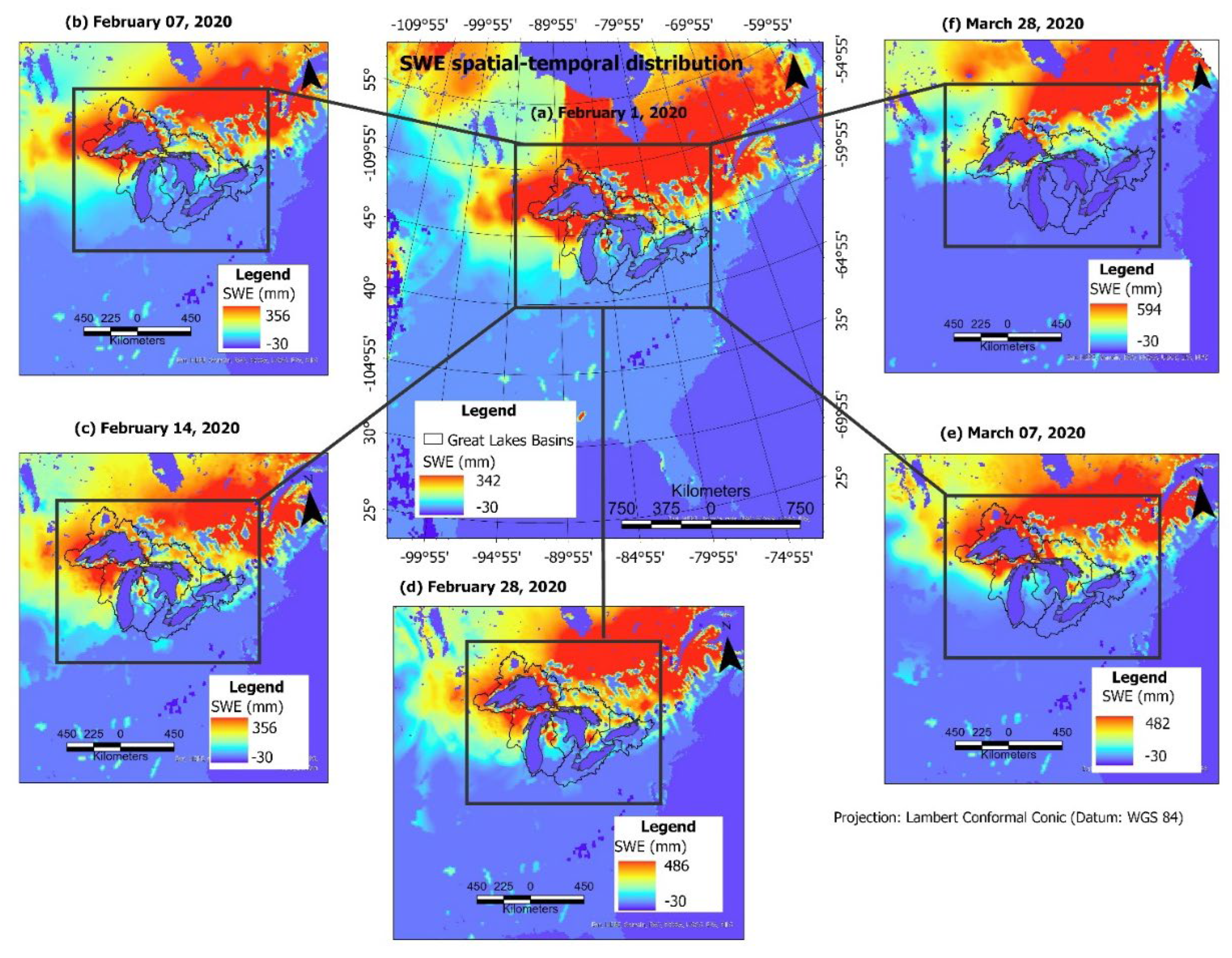
Figure 2.
Siamese UNet model. The decoders in both branches receive daily SWE as inputs; the corresponding outputs and are compared by computing their similarity using the SSIM index, which exploits changes in the spatial structure of SWE.
Figure 2.
Siamese UNet model. The decoders in both branches receive daily SWE as inputs; the corresponding outputs and are compared by computing their similarity using the SSIM index, which exploits changes in the spatial structure of SWE.
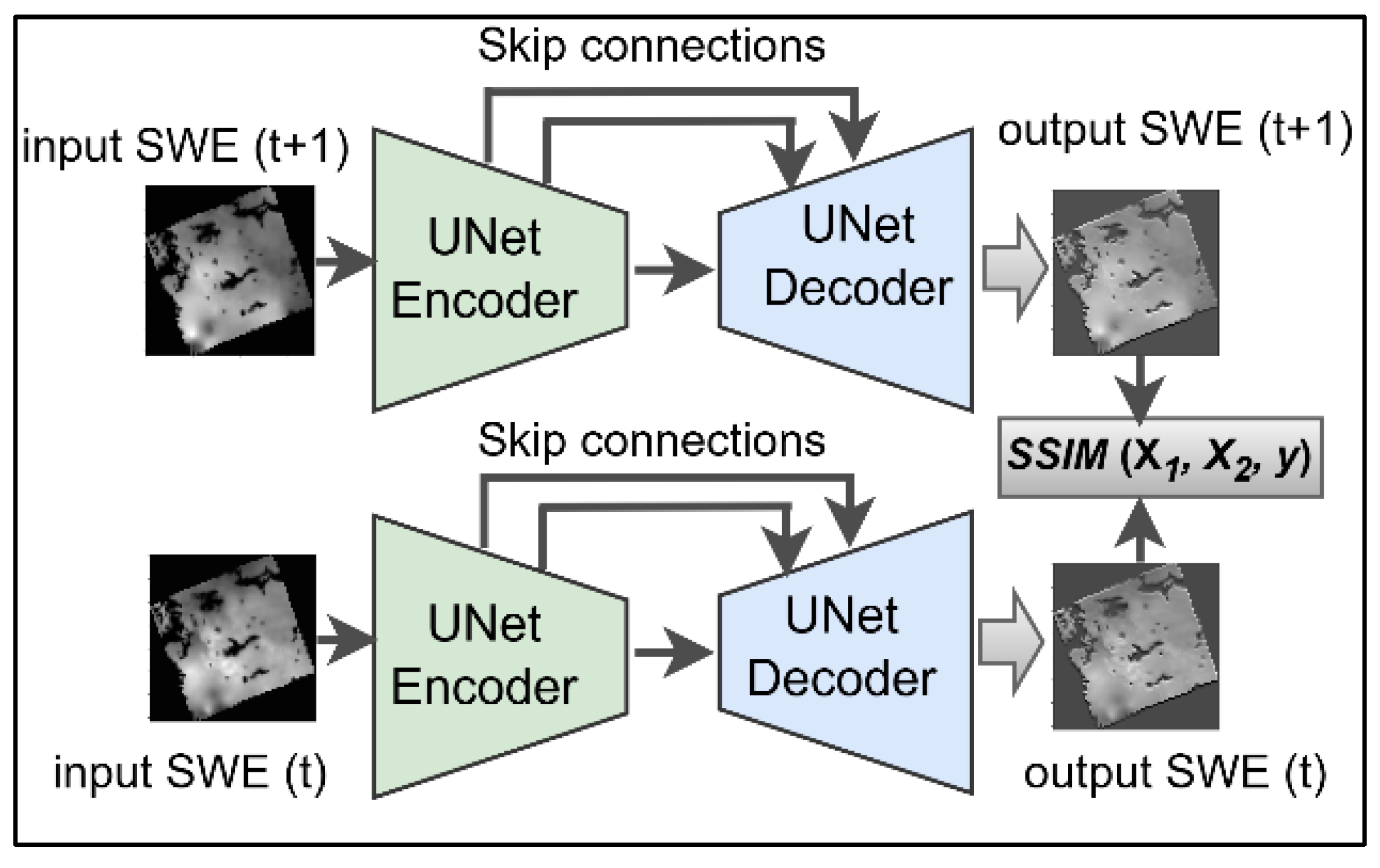
Figure 3.
Model’s confidence threshold and AUC-ROC. Optimal score for F1-score, precision, and Recall (A), and AUC-ROC for TPR and FPR. The model’s accuracy is optimal at a threshold of 0.5.
Figure 3.
Model’s confidence threshold and AUC-ROC. Optimal score for F1-score, precision, and Recall (A), and AUC-ROC for TPR and FPR. The model’s accuracy is optimal at a threshold of 0.5.
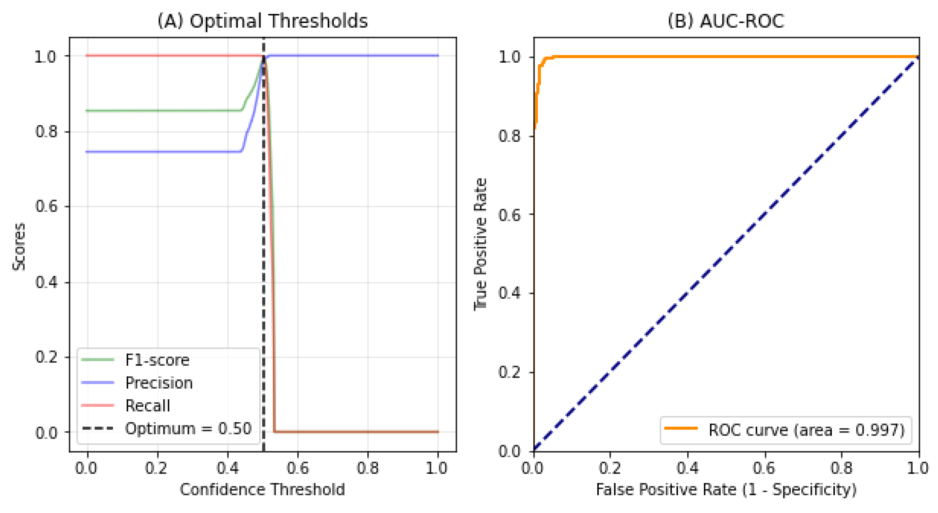
Figure 4.
Daily SWE trends over the GLB in February 1990. A – F depict observed SWE on days 19, 21, 22, 23, 21,22,23,24, and 25, respectively, as shown on the graph. Superimposed on the trend line are the linear line (orange) and 35YB (dark line). Arrows denote the direction of AA, SS, and SA events.
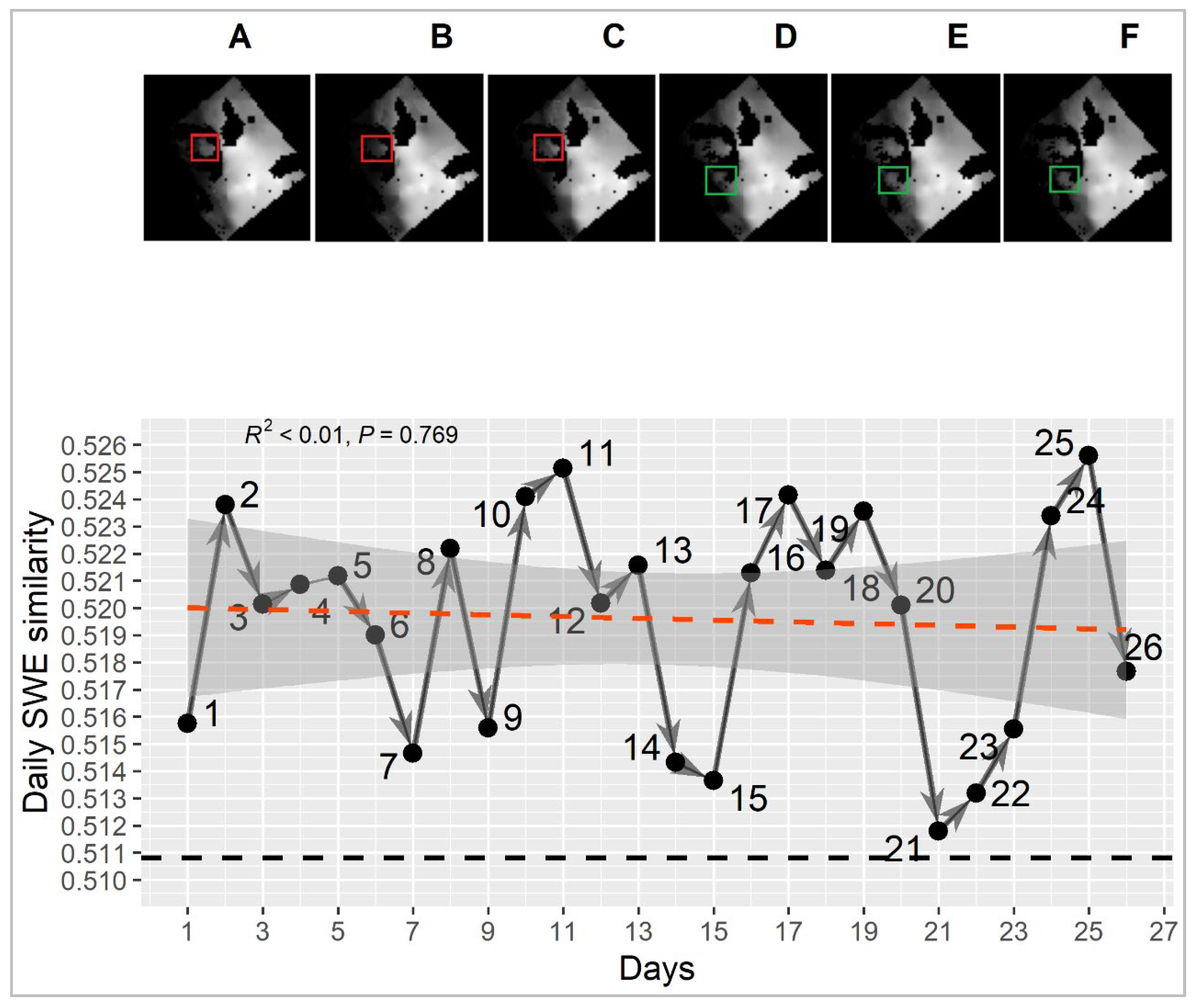
Figure 5.
Daily changes in SWE from 1989 to 1998. The blue trend lines denote daily similarity in SWE, and the red lines are linear regression estimates using the SWEsim vector.
Figure 5.
Daily changes in SWE from 1989 to 1998. The blue trend lines denote daily similarity in SWE, and the red lines are linear regression estimates using the SWEsim vector.
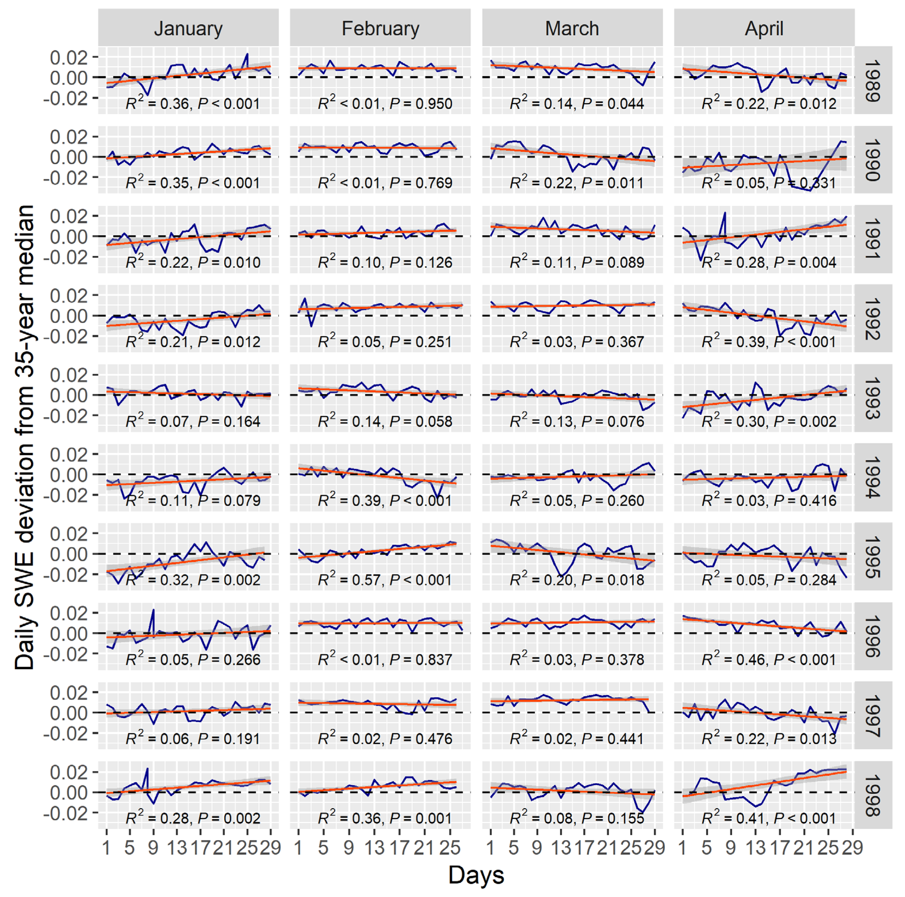
Figure 6.
Daily changes in SWE from 1999 to 2008. The blue trend lines denote daily variability in SWE, and the red lines are linear regression computed from the SWEsim vector.
Figure 6.
Daily changes in SWE from 1999 to 2008. The blue trend lines denote daily variability in SWE, and the red lines are linear regression computed from the SWEsim vector.
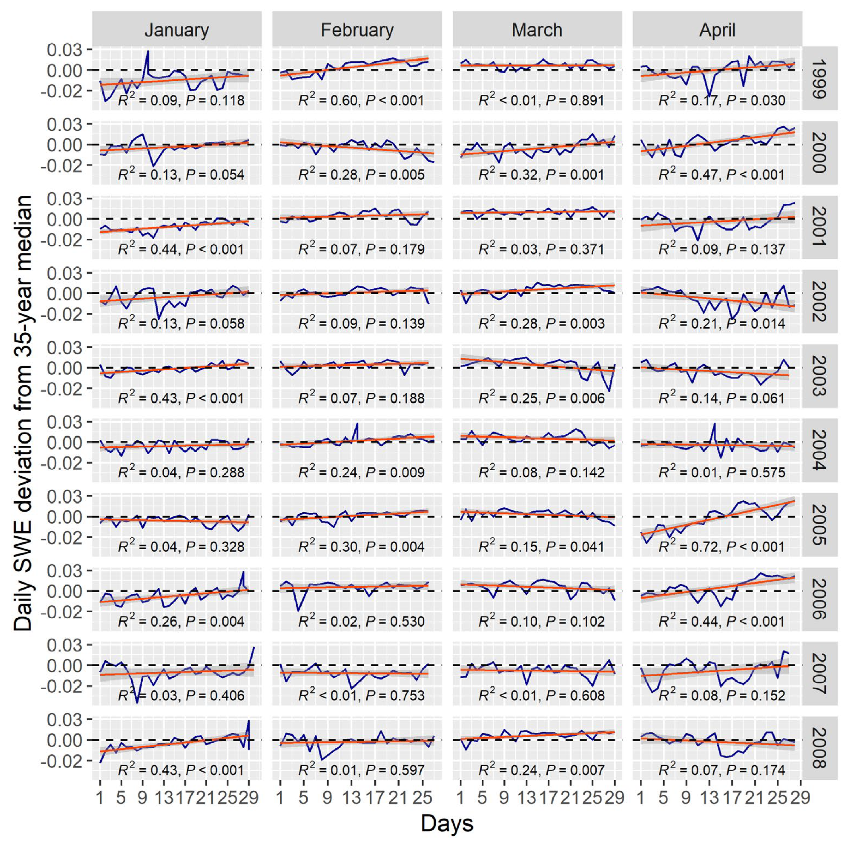
Figure 7.
Daily changes in SWE from 2009 to 2018. The blue trend lines denote daily variability in SWE, and the red lines are linear regression derived using the SWEsim vector.
Figure 7.
Daily changes in SWE from 2009 to 2018. The blue trend lines denote daily variability in SWE, and the red lines are linear regression derived using the SWEsim vector.
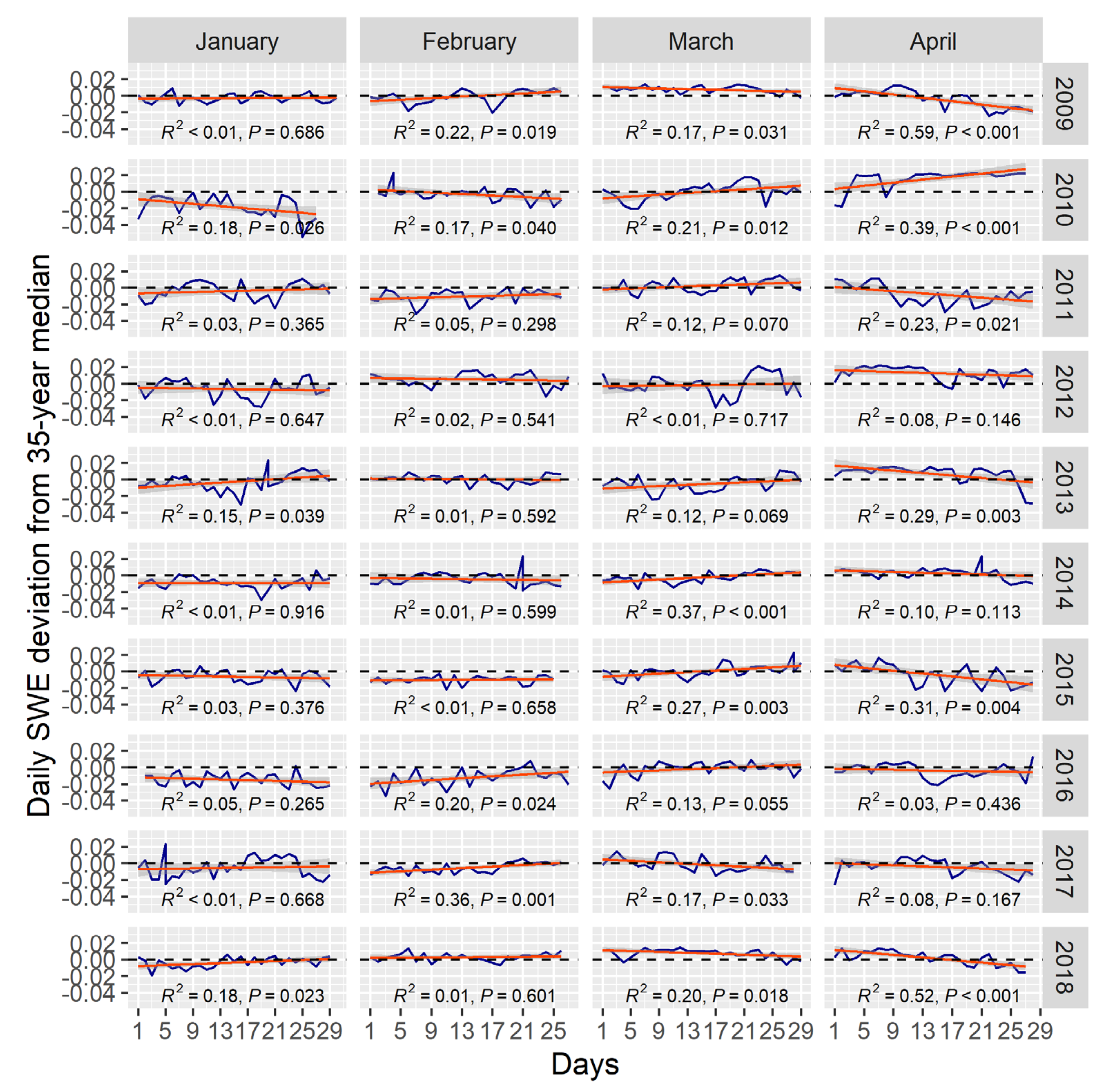
Figure 8.
SWE deviations in JFMA 1999 to 2008 compared to the 35YB SWEsim. The red dotted vertical lines mark deviations below and above the 35YB.
Figure 8.
SWE deviations in JFMA 1999 to 2008 compared to the 35YB SWEsim. The red dotted vertical lines mark deviations below and above the 35YB.
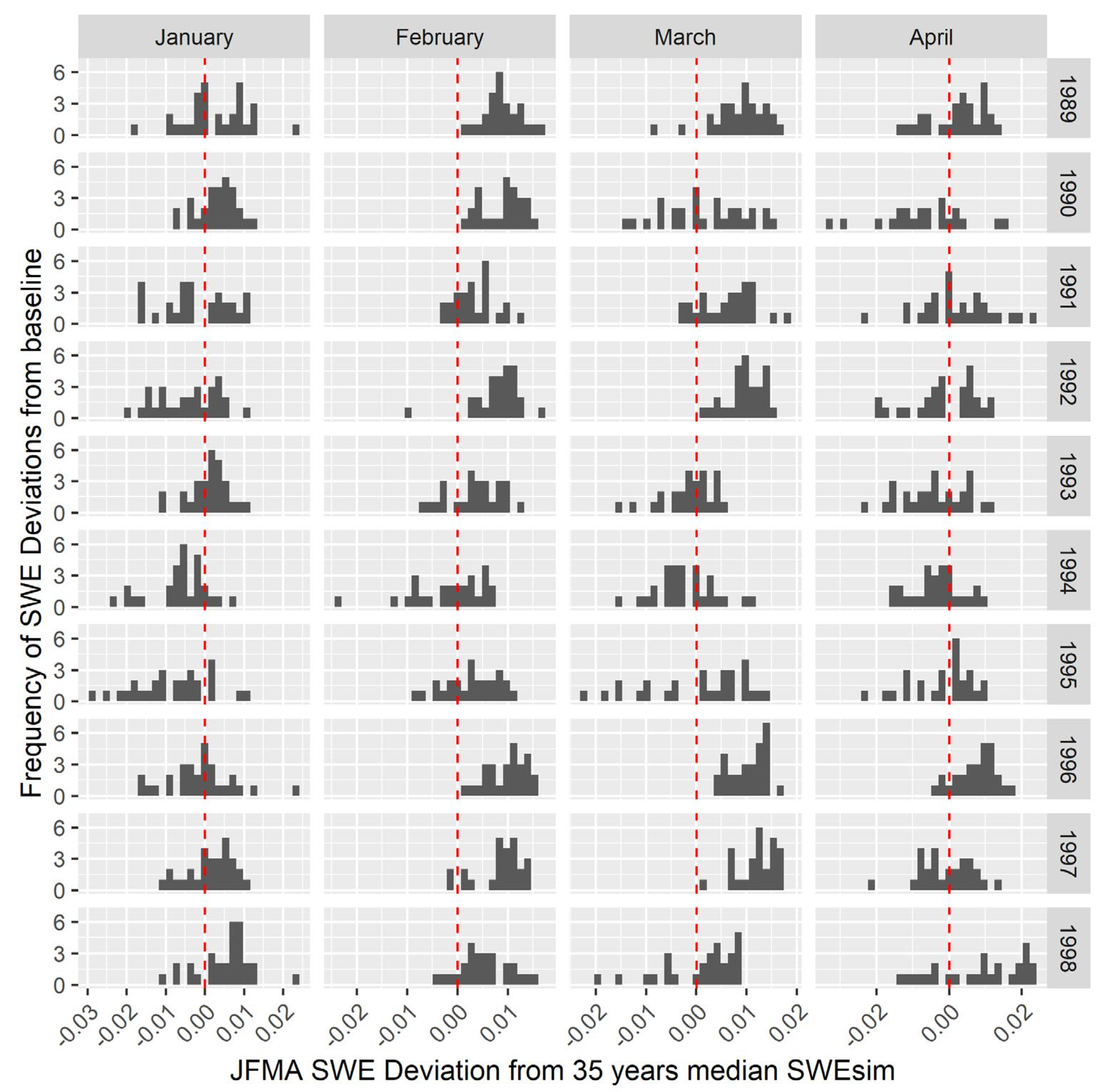
Figure 9.
SWE deviations in JFMA 1999 to 2008 compared to the 35YB SWEsim. The red dotted vertical lines mark deviations below and above the 35YB.
Figure 9.
SWE deviations in JFMA 1999 to 2008 compared to the 35YB SWEsim. The red dotted vertical lines mark deviations below and above the 35YB.
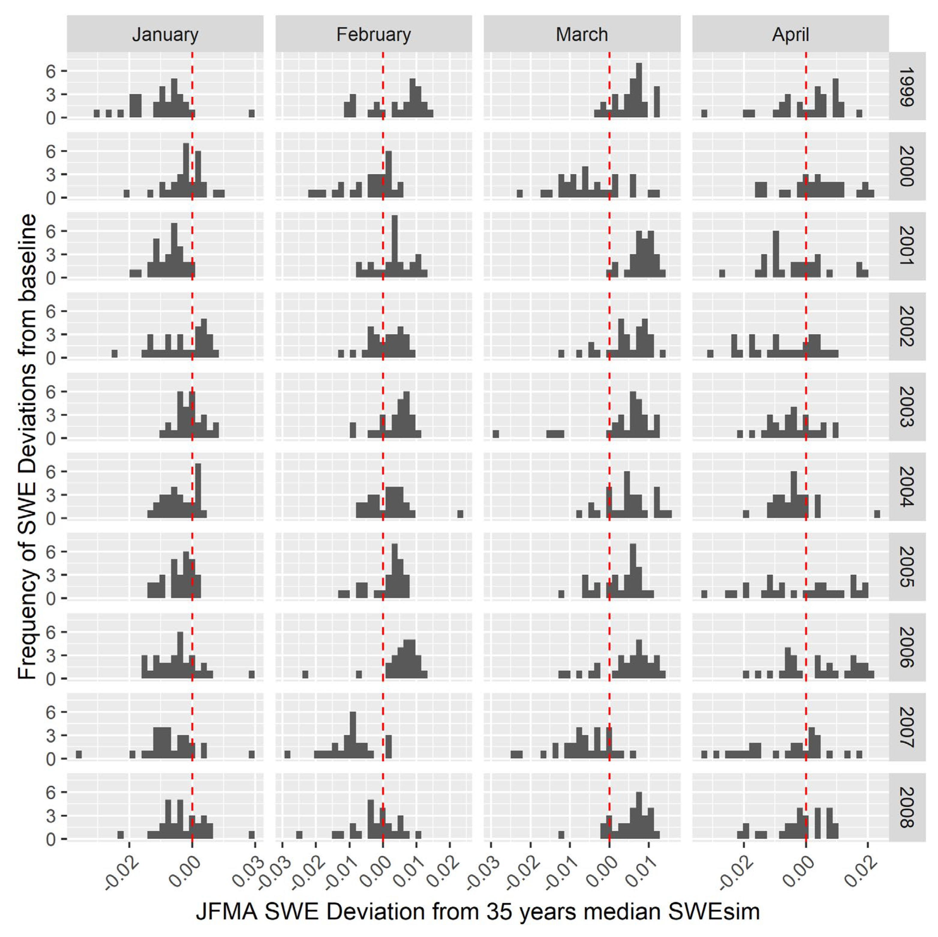
Figure 10.
SWE deviations in JFMA 2009 to 2018 compared to the 35-YB SWEsim. The red dotted vertical lines mark deviations below and above the 35-YB.
Figure 10.
SWE deviations in JFMA 2009 to 2018 compared to the 35-YB SWEsim. The red dotted vertical lines mark deviations below and above the 35-YB.
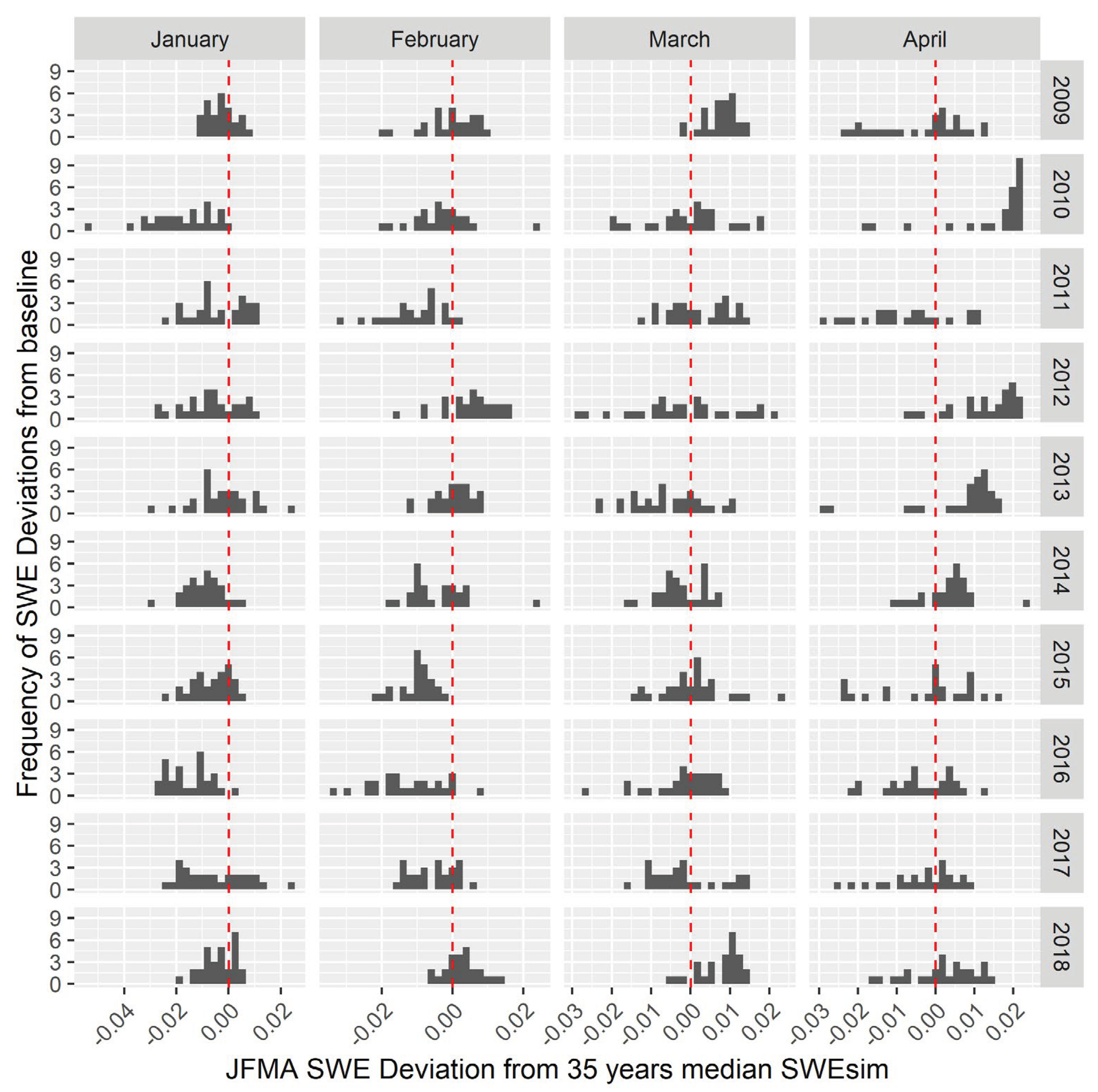

Table 1.
Model accuracy reports.
| Model Architecture |
Similarity metrics | Accuracy metrics | |||||
|---|---|---|---|---|---|---|---|
| ECD | SSIM | TPR | TNR | PR | F1 | Threshold | |
| CNN + BCE | Yes | No | 92.84 | 99.44 | 94.86 | 93.84 | 70% |
| U-Net [CL] | No | Yes | 99.91 | 92.82 | 97.59 | 98.73 | 50% |
| U-Net [BCE] | No | Yes | 100.00 | 98.37 | 87.18 | 93.15 | 80% |
Disclaimer/Publisher’s Note: The statements, opinions and data contained in all publications are solely those of the individual author(s) and contributor(s) and not of MDPI and/or the editor(s). MDPI and/or the editor(s) disclaim responsibility for any injury to people or property resulting from any ideas, methods, instructions or products referred to in the content. |
© 2026 by the authors. Licensee MDPI, Basel, Switzerland. This article is an open access article distributed under the terms and conditions of the Creative Commons Attribution (CC BY) license.
Copyright: This open access article is published under a Creative Commons CC BY 4.0 license, which permit the free download, distribution, and reuse, provided that the author and preprint are cited in any reuse.


