Structural Similarity Guided Siamese U-Net Model for Detecting Changes in Snow Water Equivalent

1. Introduction

Change detection in remotely sensed data is a frequently encountered problem. However, snow is a highly sensitive Earth cover category as it is directly and indirectly affected by diverse climate variables and feedback loops such as the snow-albedo-feedback [1]. The Earth’s cold regions are now actively being investigated to understand global warming effects on various land-cover types – tundra vegetation, snow, ice sheets, and permafrost landscape [2]. Snow represents an indispensable Northern Hemisphere (NH) land-cover component, especially during winter. Snow significantly influences the responses of flora, fauna, and entire ecosystem feedback mechanisms [2]. Melting snow produces water that feeds freshwater ecosystems and contributes to irrigation [3]. Furthermore, snow retreat time partly defines the onset of the wildfire season, especially in North American countries such as Canada. Snow parameters – SWE, snow depth, snow density, and snow spatial extent – are essential sentinels of environmental change. Due to snow's inherent sensitivity to increasing surface temperature and precipitation, these parameters have been monitored to infer the impact of climate change on the cryosphere.

The unique nature of snow sensitivity and variability poses challenges to detecting and attributing change that is linked to snow responses for forcing agents [4]. Consequently, spurious change associated with natural internal variability in snow signals is likely to be detected by less robust algorithms as change scenarios (false change). Despite this fundamental challenge in modeling and detecting change in snow, there has been progress in characterizing trends in snow water equivalent (SWE), snow depth (SD), snow cover extent (SE) [5], evaluating snow cover extent and properties [6].

One peculiar trend in the methods for snow parameter study is the adoption of reference periods and the use of arithmetic averaging techniques on time series of snow observations. Additionally, most of the studies consider the March temporal window in which SWE and snow depth are at the peak. For example, March snow data have been employed to discover declining SWE trends in Eastern and Western Canada [7]. Similarly, Pulliainen et al. [5] used March GlobSnow data to quantify snow mass across the Northern Hemisphere and discovered declining trends Raisanen [8] analyzed changes in March mean SWE in reanalysis data. While these methods yield important insights into snow trends, arithmetic averaging could amplify the modifiable areal unit problem wherein changing data resolution leads to varying results. Furthermore, general atmospheric cycles such as the Pacific/North America Oscillation, Pacific Decadal Oscillation, Arctic Oscillation, and El-Nino Southern Oscillation can result in climate regime shifts that may not be challenging to detect by studying SWE for a particular month [9,10] Therefore, analyzing snow trends in other temporal windows (January, February, March, and April) will provide a wealth of information on the evolution of the cryosphere’s response to natural climate cycles and global warming.

This study is therefore focused on three primary objectives: (a) to demonstrate Siamese U-Net's effectiveness for detecting seasonal changes in snow, (b) to illustrate the utility of computer vision metrics for comparing SWE similarity within a deep learning model architecture, and (c) to use Siamese U-Net's predictions to estimate decadal changes in SWE. To our knowledge, this research represents the most recent modification of the UNet’s architecture to incorporate the SSIM index for high temporal resolution analysis of SWE trends in the Northern Hemisphere.

1.1. Related Work and Recent Progress

1.1.1. Siamese Models for Pattern Comparison

The Siamese model incorporates a parameter-sharing paradigm, resulting in “twin models” learning an identical function to compare a pair of data points. The origin of the Siamese network for pattern comparison network can be found in [11]. Therein, the authors conceived a fully connected neural network architecture for comparing signatures to detect fraud. A convolutional Siamese network was later introduced to circumvent the limitations of fully connected networks in image comparison tasks. The model’s architecture employs the classical convolutional neural network (CNN) as the backbone model. Therefore, the pattern comparison task is executed using 1-D feature vectors in the models’ last layers. However, this comes with certain limitations. Feature vectors derived from 2-D feature maps in higher layers of deep learning models encode global patterns. As a result, 1-D vectors lack contextual and local information that encodes spatial variability in images. Fully convolutional CNN models are potential algorithms for addressing this limitation.

The U-Net, a fully convolutional CNN first introduced in [12]. The model excelled at tasks involving medical image segmentation. Several sophisticated variants of the U-Net model have been widely applied across diverse tasks. For example, the residual U-Net which uses skip connections, Dense U-Net, and Attention U-Net which incorporate attention modules [13,14,15]. More recently, multiscale attention transformer networks have been introduced to detect change [16,17,18]. The inherent and key defining attributes of U-Net models are fully convolutional feature extraction, skip or residual connections, and an Encoder-Decoder module. Unlike CNNs with 1-D dense layers, fully convolutional models retain the spatial information that characterizes local structures in images. Skip or residual connections further ensure that the spatial information is not significantly diluted as the network propagates forward [19]. In other words, residual connections pass on spatial signals that define key image elements that otherwise would have been lost in previous layers, making them accessible to succeeding layers of the model.

With the Decoder-Encoder architecture, the model learns a mapping function that simultaneously deconstructs and reconstructs the underlying data. It is worth noting that the reconstruction pipeline could be challenging to efficiently attain without the fully convolutional architecture and skip connection module [19]. Such a learning framework has important implications for pattern recognition and change detection or image content similarity analysis. By simultaneously learning image deconstruction and reconstruction mapping functions, the model implicitly understands both spatial processes that deteriorate images (e.g., high temperatures in the case of SWE) as well as those that form images (e.g., snowfall and sub-zero temperatures for SWE) at spatial scales constrained to the field of view of filters or kernels in various layers of the model. The U-Net architecture therefore has the potential to effectively analyze image content. For example, a Siamese network has been proven to detect change [20].

1.1.2. Progress in Snow Parameter Trend Analysis

Point-based monitoring of snow depth, snow density, and SWE dominated the cryosphere investigations until 1979 when the European Space Agency launched a space-borne microwave remote sensing satellite mission to collect gridded snow data [21]. Point-based measurements provide accurate estimates of snow parameters and have been utilized to validate satellite observations and reanalysis datasets. Unfortunately, a conspicuous limitation inherent in all point observations is their inability to effectively represent the spatial structure (spatial configuration) exhibited by spatial patterns generated by spatial-temporal processes. Consequently, gridded data have been derived from point-wise measurements to study snow trends [22]. Similarly, gridded snow data was deployed to study SWE and Global Climate Model evaluation [7,23]. Moreover, changes in the North American snowpacks have been effectively documented using SMMR and SSM/I passive microwave instruments onboard satellites [24].

It is important to emphasize that regardless of the data capture technology or method, snow exhibits an intrinsic internal and interannual variability which may not be related to underlying climate anomalies, and anthropogenic forcing agents [4,25]. Also, the uncertainties surrounding snow data generating models, including reanalysis datasets have been well-documented. For instance, there are uncertainties associated with using an ensemble of models to estimate SWE in North America [26]. The direct consequence of these data-related challenges is that methods that are invariant to noise, internal variability, and seasonal patterns in snow are key to obtaining accurate estimates of changes in snow parameters. Computer vision metrics and deep learning methods are crucial tools for addressing associated non-significant changes in spatial patterns and have shown promising potential [27]. For instance, CW-SSIM and SSIM have been shown to effectively detect daily SWE changes observed in April [28].

2. Materials and Methods

2.1. SWE Data and Study Are

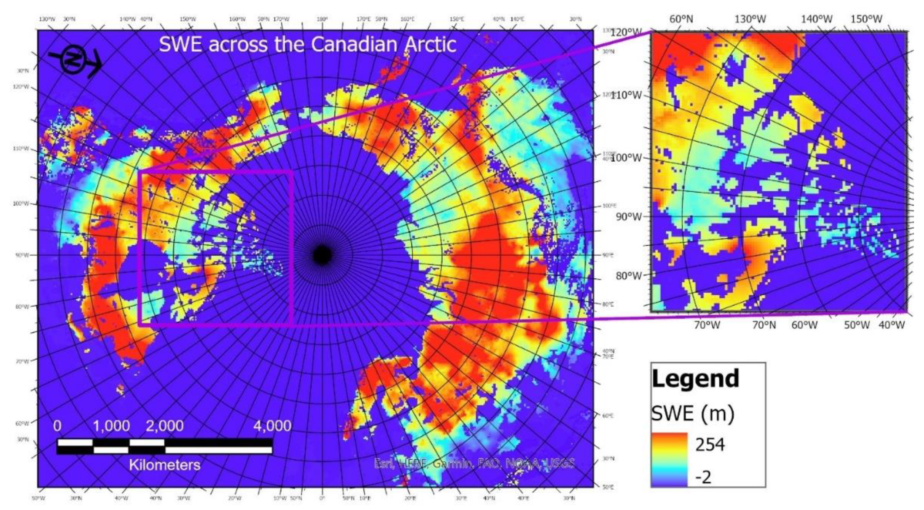
Although about 65% of the Canadian land mass is covered by snow during the winter [29], it is important to select a location with a high fraction of snow cover. The data spatial extent of the study area covers the cold regions of Canada (Alberta, Yukon, and Northwest Territories), and spans latitudes 60^oN and 70^oN. Snow arrives early in these regions and persists for longer days than in many parts of Canada. Thus, a high percentage of snow cover is sampled by Earth Observation instruments, making snow data accessible for deep learning-based modeling frameworks. GlobSnow’s version 3.0 SWE data is utilized to develop the model. The data covers the winter seasons from 1979 to 2018 and through January to April. In Figure 1, we present a SWE map to illustrate the spatial distribution of SWE in Canada during winter. It can be observed that the cold regions (shown in the pink rectangle) depict spatially varying SWE interspersed with water bodies (Lakes, Rivers, and Sea/Ocean). It can be observed The Great Bear, Great Slave Lakes' surroundings, Eastern, and Southern parts of Lake Ontario have elevated levels of SWE.

Figure 1. SWE distribution across the cold regions of Canada. Negative values (i.e., -1 and -2) denote water and mountain areas as the GlobSnow data does not cover these features.

Figure 1. SWE distribution across the cold regions of Canada. Negative values (i.e., -1 and -2) denote water and mountain areas as the GlobSnow data does not cover these features.

2.2. SWE Data Processing

The SWE data was downloaded from the repository using a script to automate the process. Further, the data was re-projected and clipped to the spatial extent of the study area using the GDAL library. All SWE data in which 50% of the area had no snow were discarded. This spatial discontinuity in SWE data was common in April. Mountainous terrains and water bodies are represented using negative numbers (e.g., -1 or -2). We replaced negative values with zeroes and used the StandardScaler function in Scikit Learn to scale the SWE values to range between 0 and 1.

2.3. Siamese U-Net Models’ Architecture

The Siamese U-Net architecture is presented in Figure 3. The Siamese network allows the model to learn shared feature representations from two input images. At the same time, the U-Net with encoder-decoder architecture and skip connections simultaneously facilitates the learning of significant features for SWE representation and reconstruction. Thus, the Siamese U-Net network learns spatial structures that characterize SWE distribution and spatial processes generating SWE. We note that though the temporal resolution of the data is high (i.e., daily), the spatial resolution is coarse. Therefore, the choice of the filter (kernel) is crucial for accurate SWE detection. The receptive field (RF) of deep learning models tends to increase by several folds with layer depth, culminating in higher layers having relatively high RF. This necessitates a thoughtful choice of filter size. Beginning feature extraction with a large filter (e.g., 5 × 5) will result in the RF growing extensively in deeper layers. Lower layers of the model extract low-level features which encode more local information whereas higher layers tend to extract abstract or global features. Thus, smaller filters will slow the rapid growth of the RF leading to the extraction of fine-grained features. We therefore adopted a 3 × 3 filter.

2.4. Training Data and SWE Labeling

Before labeling the SWE data, a thorough visual inspection was conducted to discern the spatial-temporal variability of daily SWE. We discovered that SWE data that differ by 1 day tend to vary locally; however, global differences are less pronounced. Therefore, 2 SWE maps were labeled as positive pairs (No Change) if their sampling interval was 1 day. Conversely, a pair of SWE maps were labeled negative pairs if their sampling dates were 2 or more days apart. We note that the inherent spatial-temporal variability of snow parameters renders it challenging to objectively dichotomize a pair of SWE maps. For example, SWE maps in April sometimes appeared to be largely different despite being sampled at 1-day intervals. It is also important to reiterate that there are timestamps in which SWE maps were 2 or more days apart that could not be distinguished, especially between February and March. To circumvent these challenges, the SSIM index was adapted to objectively label the data, with support from human inspection.

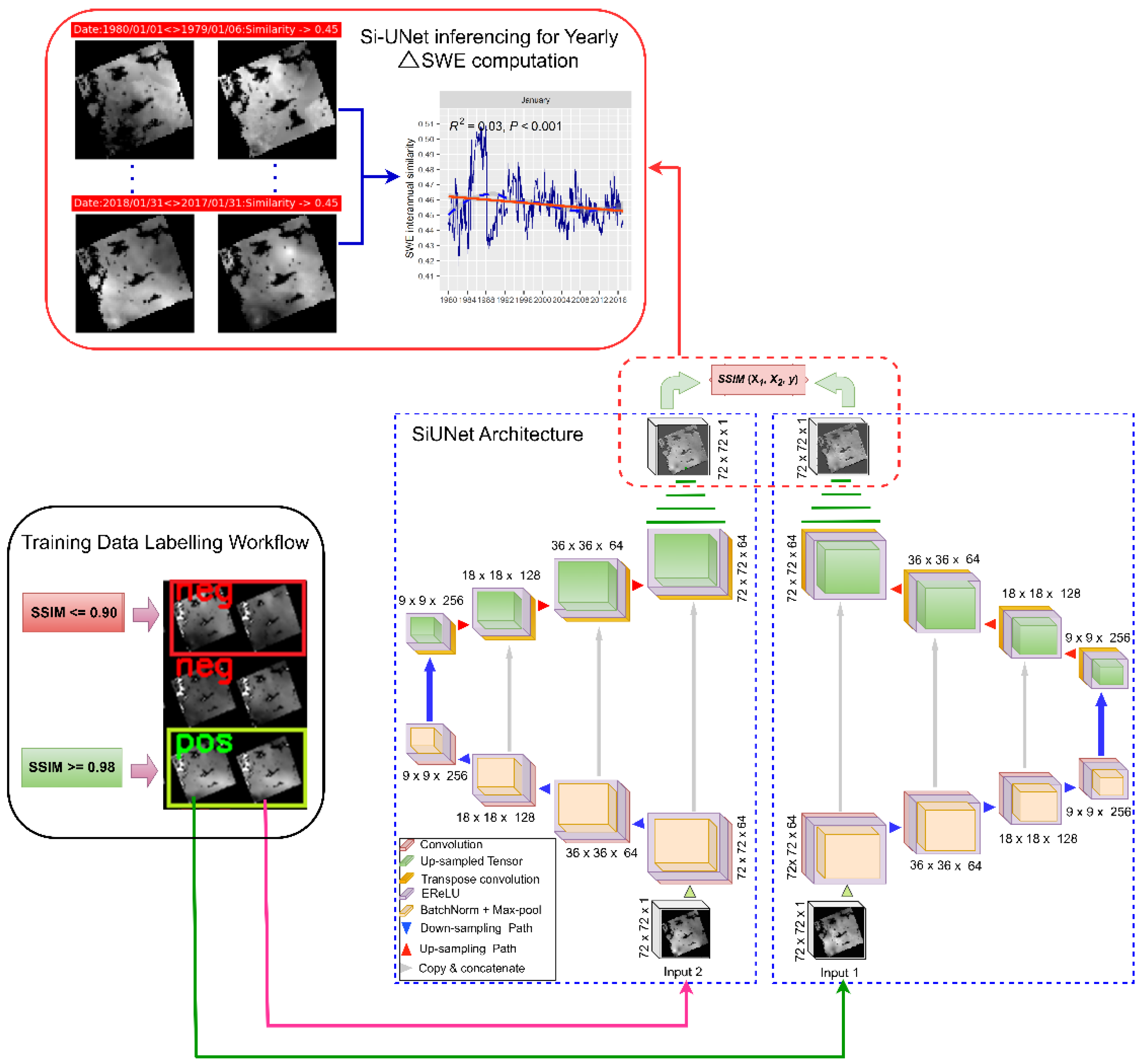
To empirically derive a threshold at which the SSIM index estimates of SWE similarity coincide with human judgment, we examined the similarity distribution of SWE data over a range of SSIM index values. At SSIM index values >= 0.98, SWE map pairs are similar and could not be easily dichotomized by human observers. Contrarily, SSIM values <= 0.9 were characteristics of SWE map pairs that are easily distinguishable (i.e., changed/different maps). Accordingly, these SSIM index values are adopted as threshold values for dichotomizing SWE pairs as positive (i.e., No Change), and Negative (i.e., Change). The SWE map pairs with SSIM values ranging from 0.91 – 0.97 were excluded from the training sample to avoid confusion during model fitting. The data labeling and concept framework for the proposed Si-UNet model with SWE over the cold regions of Canada is shown in Figure 2.

Figure 2. Siamese U-Net architecture, data labeling workflow, model training, and inferencing. The labeled 2D pair of SWE maps are passed to the pre-trained model for deconstruction and reconstruction by the Encoder and Decoder, respectively; the reconstructed SWE maps are compared to derive ΔSWE vector using the SSIM index as a scoring metric for SWE similarity.

Figure 2. Siamese U-Net architecture, data labeling workflow, model training, and inferencing. The labeled 2D pair of SWE maps are passed to the pre-trained model for deconstruction and reconstruction by the Encoder and Decoder, respectively; the reconstructed SWE maps are compared to derive ΔSWE vector using the SSIM index as a scoring metric for SWE similarity.

2.5. The SSIM Index Properties

The expression for the SSIM index, proposed by Wang et al. [30] is given below.

$$SSIM\left(x,y\right)={\displaystyle \frac{\left(2{\mathrm{\mu }}_x{\mathrm{\mu }}_y+C_1\right)\left(2{\sigma }_{xy}+C_2\right)}{\left({\mathrm{\mu }}_x^2{+\mathrm{\mu }}_y^2+C_1\right)\left({\sigma }_x^2+{\sigma }_y^2+C_2\right)}}$$

(1)

${\mu }_x{ \mathrm{a}\mathrm{n}\mathrm{d} \mu }_{y }$ are represent the mean of a block of pixels in image x and y, respectively;  ${\sigma }_x^2$, ${\sigma }_y^2$ are respectively the variance of x and y while ${\sigma }_{xy}$ are x and y covariance terms; $C_1 {\mathrm{a}\mathrm{n}\mathrm{d} C}_2$ are stabilizing constants to account for the saturation effects of the human visual system.

The SSIM index exhibits symmetry – $SSIM\left(x,y\right)=SSIM\left(y,x\right).$ Thus, the SSIM index value is insensitive to the order in which the similarity of the output of the 2D SWE generated by Si-UNet is evaluated. Additionally, the upper bound of the SSIM index, $SSIM\left(x,y\right)=1$ is attained if and only if (i.i.f) two pairs of SWE maps are identical copies. Contrarily, the lower bound of the SSIM index, $SSIM\left(x,y\right)=0$ would occur when a pair of SWE maps are distinctively opposite pairs (e.g., snow versus zero-snow area). Nonetheless, given the temporal dimension of the data, and the magnitude of inherent spatial variability in the distribution of SWE, it is highly improbable that these two scenarios will ever be established for any bi-temporal SWE maps. Consequently, the SSIM index value is constrained to follow the expression $0\le SSIM\le 1$. This property renders the optimization task via contrastive loss with $m=1$ an effective technique and corroborates the adoption of the SSIM index.

2.6. The Contrastive Loss Function

Contrastive loss has been proven to be effective for learning tasks that involve dichotomizing a pair of data points. The learning objective compels similar data point pairs to attract a higher similarity score and assigns a lower score to a set of dissimilar data pairs [31]. This aligns with the notion of maximizing the SSIM index value for similar (No Change SWE) and minimizing the SSIM index value for unlike pairs (Change SWE) as illustrated using the notations below:

$$\partial \left(x^i,x^j\right)=\left\{\begin{array}{c}\max |SSIM\left(x^i,x^j\right)|, i=j\\ m\mathrm{in} |SSIM\left(x^i,x^j\right)|,i \ne j\end{array}\right.$$

(2)

where $i,j$ are indexes into a set of 2D feature maps, and $SSIM\left(·\right)$ denotes the SSIM index.

The contrastive loss function written to incorporate the SSIM index is given as follows:

$$L_c=(1-Y){\displaystyle \frac{1}{2}}(SSIM\left(x,y\right){)}^2+\left(Y\right){\displaystyle \frac{1}{2}} {\left\{\max \left(m-SSIM\left(x,y\right), 0\right)\right\}}^2(3)$$

(3)

where $L_c$ denotes contrastive loss, $m$ and $SSIM$ are margin and SSIM index, respectively; $x,y$ denote a pair of SWE images and $Y$ represents image pair labels. Note that for positive pairs (No Change SWE), $Y=1$ (i.e., $Y=1\left|\right\{i=j\}$) and for negative pairs (Change SWE), $Y=0$ (i.e., $Y=0\left|\right\{i \ne j\}$). We note that the SSIM’s upper bound is 1 and this aligns with the margin parameter $m=1,$ often adopted for the contrastive loss function. In the next section, we decompose the contrastive loss to illuminate how the SSIM index fits into the objective function’s optimization paradigm.

2.7. Learning with the Contrastive Loss Function and SSIM Index

It is worth noting that at each epoch, the SSIM index values are passed to the contractive loss function for optimization. By substituting $m=1$ into the second component of the contrastive loss function with the SSIM index, the expressions below are yielded:

$$m-SSIM\left(x,y\right)=\mathrm{m}-{\displaystyle \frac{\left(2{\mathrm{\mu }}_x{\mathrm{\mu }}_y+C_1\right)\left(2{\sigma }_{xy}+C_2\right)}{\left({\mathrm{\mu }}_x^2{+\mathrm{\mu }}_y^2+C_1\right)\left({\sigma }_x^2+{\sigma }_y^2+C_2\right)}}$$

(4)

$$1-SSIM\left(x,y\right)=1-{\displaystyle \frac{\left(2{\mathrm{\mu }}_x{\mathrm{\mu }}_y+C_1\right)\left(2{\sigma }_{xy}+C_2\right)}{\left({\mathrm{\mu }}_x^2{+\mathrm{\mu }}_y^2+C_1\right)\left({\sigma }_x^2+{\sigma }_y^2+C_2\right)}}$$

(5)

The SSIM index expression, after $x$ and $y$ are mean-reduced, is simplified as follows:

$$1-SSIM\left(x,y\right)=1-{\displaystyle \frac{2{\sigma }_{xy}+C_2}{{\sigma }_x^2+{\sigma }_y^2+C_2}}$$

(6)

Thus, the covariance term ${\sigma }_{xy}$, which encodes similarities or differences in spatial structure between a pair of SWE maps being compared is amplified.

Given the “No Change SWE” scenario, $Y=1$ (i.e., $Y=1\left|\right\{i=j\}$), the first half of the contrastive loss expression (equation 3), $(1-Y){\displaystyle \frac{1}{2}}(SSIM\left(x,y\right){)}^2$ is nullified as it evaluates to 0; the second component, $\left(Y\right){\displaystyle \frac{1}{2}} {\left\{max(m-sim, 0)\right\}}^2$ is then optimized as illustrated below.

$$L_c=\left(1\right){\displaystyle \frac{1}{2}} {\left\{max(1-SSIM\left(x,y\right), 0)\right\}}^2$$

(7)

Therefore, if the image pairs are true “No Change” pairs, the SSIM value is expected to be high (i.e., near 1). Consequently, according to this equation, the model’s loss will reduce significantly (i.e., $L_c\approx 0$) for SSIM values close to 1.

For scenarios of “Change SWE”, $Y=0$ (i.e., $Y=0\left|\right\{i \ne j\}$), the first component in equation 3, $(1-Y){\displaystyle \frac{1}{2}}(SSIM\left(x,y\right){)}^2$ is optimized while $\left(Y\right){\displaystyle \frac{1}{2}} {\left\{max(m-SSIM\left(x,y\right), 0)\right\}}^2$ evaluates to zero and is nullified accordingly.

$$L_c=(1-0){\displaystyle \frac{1}{2}}(SSIM\left(x,y\right){)}^2$$

(8)

If the image pairs are true “Change SWE” pairs, the SSIM value is expected to be very low (i.e., close to 0). As a result, the model’s loss will again be low (i.e., $L_c\approx 0$) for SSIM values near 0. Intuitively, according to the constrastive loss function, it follows that the model’s losses will increase i.i.f the computed SSIM value is high (near 1) but image pairs are labelled as “Change SWE” (False Change). In contrast, the model’s losses will increase i.i.f the image pairs are labeled as positive (“No Change”) but the SSIM value turns out to be low (False No Change).

2.8. Accuracy Metrics

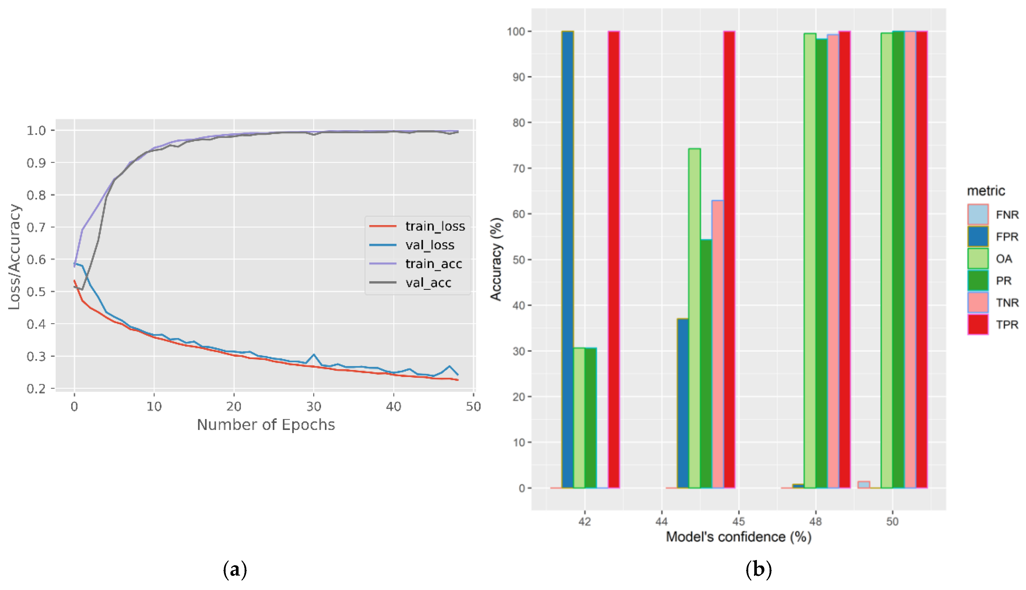
The Si-UNet models' training history and performance at inference are shown in Figure 3a,b. We computed the true positive rate (TPR), true negative rate (TNR), false positive rate (FPR), false negative rate (FNR), and overall accuracy (OA) to assess the models’ prediction of SWE change. The equations are presented in Appendix A2. The model’s accuracy is evaluated at a threshold from 40% – 50%. SWE data from 1979 to 2001 were employed for model development whereas data from 2002 to 2018 form an independent validation sample. Furthermore, qualitative analysis and visualizations of change maps were employed to interrogate the model's change detection capabilities.

Figure 3. Training history for the Siamese U-Net model and accuracy metrics.

Figure 3. Training history for the Siamese U-Net model and accuracy metrics.

2.9. Deriving Time-Series SWE Change Vectors

Once trained and independently validated, the Si-UNet can be deployed to derive time-series change vectors for daily, monthly, and yearly SWE. To compute yearly change, SWE data in corresponding months are compared across succeeding years using the Si-UNet model to compute similarity values. For example, to derive ΔSWE trends for January from 1979 and 2018, Si-Unet receives time series SWE data in January and outputs ΔSWE by sequentially pairing the yearly SWE maps as follows: SWE₁₉₇₉ versus SWE_1980, SWE₁₉₈₀ versus SWE_1981, SWE₁₉₈₁ versus SWE₁₉₈₂ until the end of the time-series length (i.e., 2018). Reformulating the comparison equation in terms of mathematical notations yields a vector of ΔSWE as follows:

$$\overrightarrow{{SWE}_{\left\{Z_i\dots Z_n\right\}}}=\mathrm{S}\mathrm{i}\mathrm{U}\mathrm{N}\mathrm{e}\mathrm{t}\left\{{SWE}_{Z_i}\left(j_1,j_2,j_3\dots j_{31}\right),{SWE}_{Z_{i+1} }\left(j_1,j_2,j_3\dots j_{31}\right)\right\}$$

(9)

where $j_1$to $j_{31}$ denote January 1 to January 31 SWE data whereas $Z$ represents year. Such a comparison compels Si-UNet to answer a visual question of whether SWE data, sampled in the most recent year, $Z_{i }$and the preceding year, $Z_{i-1}$ are different. More specifically, the model answers the question: is the SWE data observed on 1^st January 2017 significantly different from the SWE data observed on 1^st January 2018? The Mann-Kendal trend test and linear regression were performed on the resultant $\mathrm{S}\mathrm{W}\mathrm{E}$ vector to portray trends in SWE [24,32].

3. Results

3.1. A comparison of Monthly Changes in SWE Distribution Over 5 Years

Figure 5, Figure 6 and Figure 7 present a combined violin and box plot for the similarity distribution of SWE derived from a comparison of SWE between consecutive years, from January through April. Higher SWE values signify less significant change; conversely, lower values reflect pronounced changes in SWE between the years compared. Due to the temporal resolution of the GlobSnow data between 1979 and 1987, ΔSWE vector of length n ≈ 14 days for each month. The ΔSWE vectors after 1987 have an average length n ≈ 29 days.

3.2. SWE Distribution – 1980 to 1984

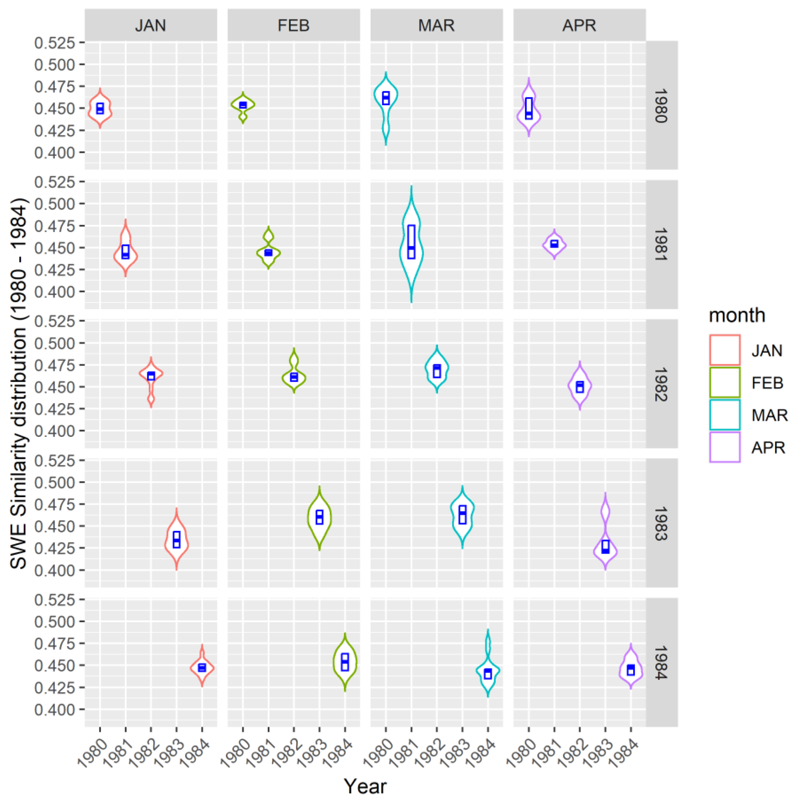
Figure 5 depicts a 5-year distribution of changes in SWE. The median ΔSWE similarity for March values appears to be the highest. Aside from 1984, all the preceding years recorded over 0.45 median similarity. April turns out to have the lowest median similarity. While all the months portray prominent dispersion over the years, ΔSWE in February appears to be more uniform from 1980 to 1982.

Figure 4. SWE distribution for years 1980 - 1984. The SWE distribution captures the years in which mean precipitation and temperature anomalies were low.

Figure 4. SWE distribution for years 1980 - 1984. The SWE distribution captures the years in which mean precipitation and temperature anomalies were low.

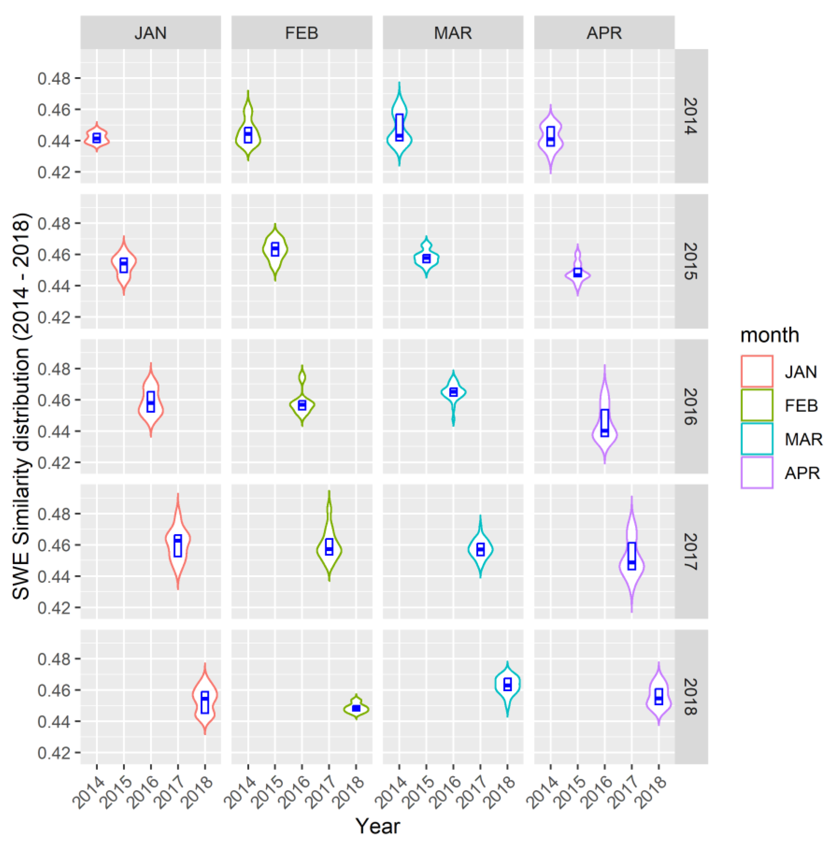
3.3. SWE Distribution – 2014 to 2018

Figure 7 summarizes SWE distribution between 2014 and 2018. As can be discerned from the figure, 2014 incurred the lowest ΔSWE values for all the months (i.e., January – April). Given that the 2014 distribution is derived from a comparison between 2013 SWE data, it implies that the spatial structure characterizing the distribution of SWE in 2013 and 2014 were distinctively different. March exhibits the highest ΔSWE values followed by February and January. It is important to note, however, that January and April ΔSWE largely depict bimodal distribution with high dispersion.

Figure 5. SWE distribution for years 2014 - 2018. It can be observed that ΔSWE for January and April continues to be more dispersed; however, April ΔSWE median values were comparatively low.

Figure 5. SWE distribution for years 2014 - 2018. It can be observed that ΔSWE for January and April continues to be more dispersed; however, April ΔSWE median values were comparatively low.

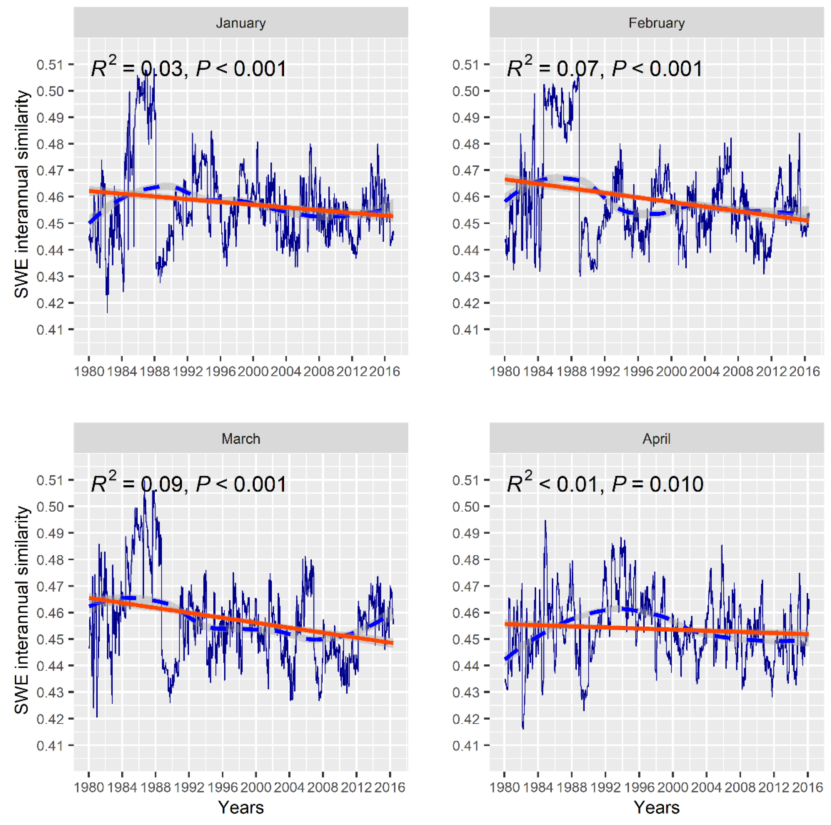
3.4. Interannual SWE Trends – 1979 to 2018

Figure 6 depicts SWE trends from 1970 to 2018. We first conducted a non-parametric Mann-Kendall test to ascertain the SWE trend's direction (positive/increasing or negative/decreasing). Further, linear regression and locally estimated scatterplot smoothing (LOESS) were fitted to the time-series data. Mann-Kendall test suggests a statistically significant negative or decreasing monotonic trend (tau < 0) in all the months. However, March incurred the highest rate of SWE decline (R² ≈ 0.1, p-value < 0.05). Table A1 (see Appendix A1) presents the statistics derived from the trend tests. The statistics – S, tau, and p-values are reported from Mann-Kendall test while the R² values are derived from linear regression. On average, ΔSWE values were higher in the earlier years of 1979 – 1988. The later years (i.e., 1988 – 2018) were dominated by low ΔSWE values.

Figure 6. A 40-year SWE trend in Canada’s cold regions from January to April. Blue dotted lines are LOESS fitting, and orange-red lines are derived from linear regression. The gray area around the trend lines denotes a 95% confidence interval.

Figure 6. A 40-year SWE trend in Canada’s cold regions from January to April. Blue dotted lines are LOESS fitting, and orange-red lines are derived from linear regression. The gray area around the trend lines denotes a 95% confidence interval.

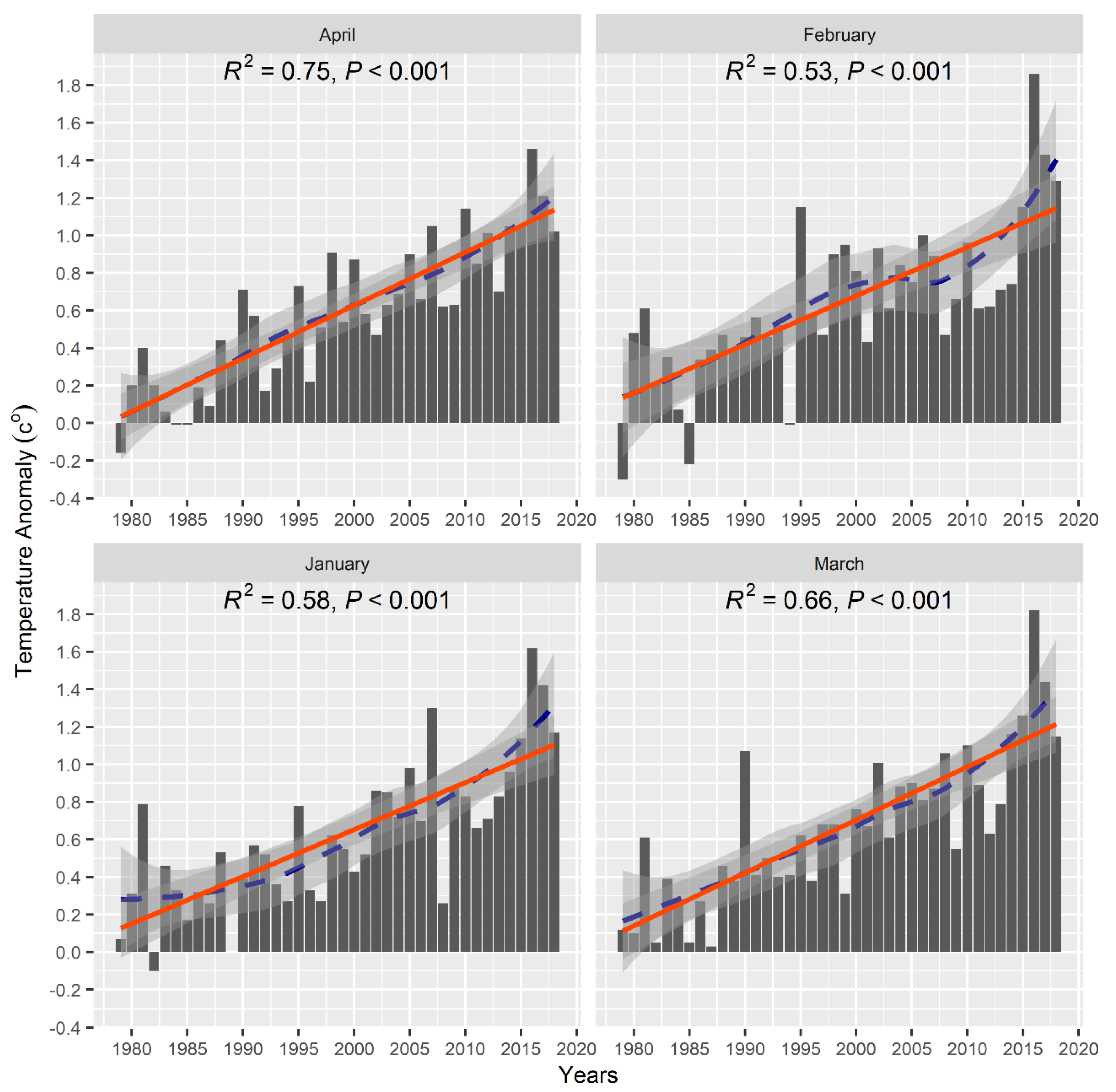
3.5. The Northern Hemisphere Temperature Anomalies

In Figure 7, we present the National Oceanic and Atmospheric Administration (NOAA) mean monthly temperature anomalies from January to April. Comparing Figure 6 and Figure 7, it can be deduced that a decreasing pattern of SWE similarity coincides with an increasing temperature anomaly. Although the temperature anomalies portray a growing trend, the lowest average monthly anomaly occurred in the first 10 years (i.e., 1979 – 1989), whereas the latter years exhibit relatively high temperature anomalies. It can be discerned that March and April have the strongest positive trends and R² of 0.66, and 0.75, respectively.

Figure 7. Land and Sea Surface Temperature anomalies in the Northern Hemisphere. The blue-dotted and the orange-red lines denote LOESS fitting, and linear regression trend estimates, respectively. The gray area around the LOESS and regression lines represents a 95% confidence interval. Positive temperature anomalies tend to dominate all the months. The earlier years (e.g., 1979 – 1989) portray negative and low positive anomalies compared to the latter years (e.g., 1990 – 2018).

Figure 7. Land and Sea Surface Temperature anomalies in the Northern Hemisphere. The blue-dotted and the orange-red lines denote LOESS fitting, and linear regression trend estimates, respectively. The gray area around the LOESS and regression lines represents a 95% confidence interval. Positive temperature anomalies tend to dominate all the months. The earlier years (e.g., 1979 – 1989) portray negative and low positive anomalies compared to the latter years (e.g., 1990 – 2018).

4. Discussion

We developed a Si-UNet to detect spatial-temporal change using GlobSnow’s SWE data across Canada’s cold Regions. We cast the change detection problem as image content similarity analysis wherein highly similar pairs of images (e.g., SWE maps) are anticipated to liberate high scores whereas dissimilar pairs of images yield low scores. Thus, a high similarity score denotes little or no significant change in SWE. Low score on the other hand is indicative of significant change in SWE. Siamese networks have been shown to extract discriminative features for pattern recognition tasks [34]. However, the challenge encountered in SWE change detection warrants modifications to the model’s architecture, and loss function. Consequently, we adopted the U-Net backbone, the SSIM index, and the contrastive loss function to capture the spatial-temporal variability between a pair of SWE images [30,35,36]. The model is guided by a computer vision metric – SSIM index to weigh structural changes higher than changes in the intensity and contrast of SWE images [30]. We further exploit this property of the SSIM index by deploying it to objectively label the training samples. This workflow, including the model’s architecture, is depicted in Figure 3. The SSIM scales out the effects of contrast and illumination variability while preserving structural differences. The structural component highly correlates with underlying spatial-temporal processes (e.g., precipitation and temperature) that largely dictate snow dynamics. We show that the model holds the potential to detect interannual changes in snow parameters. We found that a higher confidence threshold is essential for eliminating the occurrence of false positives and false negatives. At a 50% threshold, our model achieves 99% accuracy after rigorous testing using 2002 – 2018 SWE data reserved for independent validation. We estimated interannual changes in SWE by comparing yearly SWE from January to April. The larger the value of ΔSWE, the higher the similarity between a pair of SWE maps. In other words, the larger ΔSWE is, the smaller the magnitude of change between a pair of SWE maps.

The distribution of ΔSWE for January and April tends to be frequently bimodal (Figure 4 and Figure 5) and relatively more dispersive compared to February and March. The dispersion of ΔSWE in January is characteristic of the variability in snow arrival and accumulation whereas that of April is indicative of variability in yearly snow melt-off patterns. Snow begins to melt and retreat during April but tends to exhibit a spatially variable distribution [37]. The lower median ΔSWE values for all the months in April accentuate this melt-off pattern. The Si-UNet model predicts higher ΔSWE values between 1980 and 1984 (Figure 4). Conversely, lower ΔSWE values were observed between 2014 and 2018 (Figure 5). Climate change and global warming phenomena are known to significantly affect precipitation and surface temperature, which in turn, drive snowfall events [9,38,39], resulting in declining snow accumulation.

The distribution of monthly changes of SWE within each year can provide an informative insight into snow evolution in response to climate regime variability. To link the spatial-temporal variability of snow parameters to climate variables, we compared Land and Sea Surface Temperature (LSST), and precipitation anomalies reported by NOAA in the NH for the corresponding years – 1980 to 1984 and 2014 to 2018 (Figure 7) [39]. Temperature anomalies were relatively low between 1980 and 1984. Contrarily, high temperature anomalies were detected between 2014 and 2018. As expected, an inverse relationship is discernible between ΔSWE and LSST anomalies. The ΔSWE remained high from 1980 to 1984 for all the months; this temporal window corresponds with the periods in which LSST anomalies were relatively low. The values of ΔSWE, however, decreased steadily after 1988 when temperature anomalies continued to increase. These findings are consistent with extensive studies of the NH snow cover response to surface temperature [6,10,40,41].

Temperature and precipitation are key climate variables known to have a profound influence on snow dynamics [1,42]. This study finds any reasonably consistent pattern in SWE relationship with NOAA’s climate anomalies. However, there was a strong correlation between SWE decline and temperature anomalies than precipitation. Overall, precipitation in January (Figure not shown here) exhibits the strongest relationship with SWE decline. Nevertheless, it is worth noting that spatial processes such as temperature and precipitation do not act at the same spatial scales; thus, their effects on spatial patterns will require analysis at relevant scales to understand their impact on the snow regime [43].

Mann-Kendal trend test and linear regression agree with negative SWE trends from 1980 – 2018. Although all the years depict a negative or declining interannual SWE, the trend is statistically more significant in March. The Si-UNet detects the steepest SWE decline or change in March (R² $\approx$ 0.1, p-value < 0.05). All the other months portray a statistically significant reduction in SWE yet have weaker R² values. The negative trends align well with previous studies that discovered a significant reduction in SWE, SD, and SE over the NH, especially in snow-peak months such as March [22,44,45].

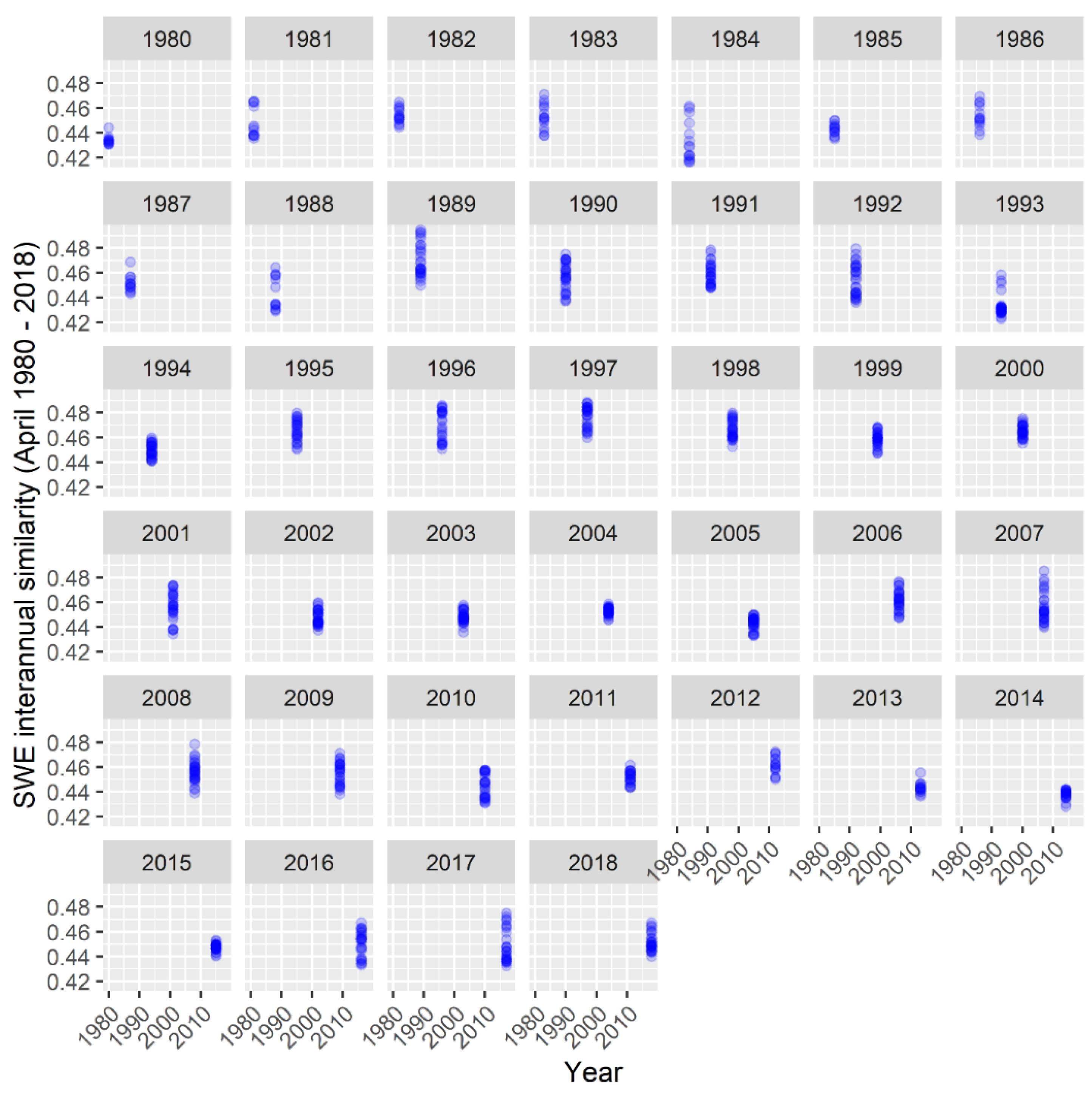
We reiterate that despite the relatively weak R² for the April SWE trend, it incurred the lowest ΔSWE values (Appendix B, Figure B1). This signifies that April SWE has been largely impacted by natural and anthropogenic climate-forcing agents [4]. Furthermore, the high spread or dispersion observed in April SWE distribution emphasizes the oscillatory impact of climate-forcing agents on snow melt-off across space and time. It has been shown that snow and ice cover in Canada is decreasing over time, with inherent seasonal and regional variability which is largely attributable to surface temperature [46]. Together, the negative slope of March ΔSWE and the lower median ΔSWE values for April portend earlier snowmelt and shorter winter season length in the NH [47,48,49]. This presents a worrying trend given that snow duration in winter is crucial for sustaining water resources particularly, in the cold regions of Canada where melting snow represents a vital source of freshwater and outdoor leisure activities such as skating [32,50].

5. Conclusions

Our study demonstrated the utility of combining computer vision and deep learning methods to detect spatial-temporal change in snow parameters. The SSIM-guided Si-UNet model detects changes in SWE with 99% accuracy at a 50% confidence threshold. Nonetheless, at lower confidence thresholds (e.g., 40 – 45%) the model yields false positives and false negatives, highlighting the challenging nature of the change detection problem in SWE. Analysis of ΔSWE and LSST reveals an inverse relationship, suggesting the impacts of temperature on SWE decline in the cold regions of Canada. This decline is more pronounced after 1988 when LSST anomalies continue to rise exponentially. March ΔSWE exhibits a strong negative trend compared to January, February, and April. However, the values of ΔSWE in April tend to be the lowest, indicating the severity of climate-forcing impacts on the snow regime in April. The distribution of ΔSWE values in January and April is more dispersive. With progressive perturbation and instability of the snow regime in January and April, ΔSWE is likely to reduce significantly, impacting the length of the winter season. We note that though the GlobSnow V3.0 data is of high temporal resolution, its coarse spatial resolution limits analysis of changes in snow at local scales. Higher spatial resolution datasets will offer more insight into changes in the snow regime and the cryosphere’s response to natural and anthropogenic climate-forcing agents. Additionally, extending this analysis to other regions in the NH will provide an informed understanding of the impact of climate-forcing agents on the cryosphere processes at broader spatial scales beyond the cold regions of Canada. The latter is the next analysis we intend to conduct in the future.

Appendix A.1

Table A1. Mann-Kendall test and linear regression statistics.

Month	N	S	tau	p-value	R2
January	1019	-3.31e+04	-6.37e-02	2.31e-03	3.0e-02
February	950	-4.38e+04	-9.72e-02	7.34e-06	7.0e-02
March	1019	-8.16e+04	-1.57e-02	5.62e-14	9.0e-02
April	940	-3.47e+04	-7.85e-02	3.13e-04	1.0e-02

Table A1. Mann-Kendall test and linear regression statistics.

Month	N	S	tau	p-value	R2
January	1019	-3.31e+04	-6.37e-02	2.31e-03	3.0e-02
February	950	-4.38e+04	-9.72e-02	7.34e-06	7.0e-02
March	1019	-8.16e+04	-1.57e-02	5.62e-14	9.0e-02
April	940	-3.47e+04	-7.85e-02	3.13e-04	1.0e-02

Appendix B.1

Figure B1. April SWE distribution from 1980 – 2018, showing ΔSWE vectors’ values as blue dots for the corresponding years.

Figure B1. April SWE distribution from 1980 – 2018, showing ΔSWE vectors’ values as blue dots for the corresponding years.

References

- C. W. Thackeray, C. Derksen, C. G. Fletcher, and A. Hall, “Snow and Climate: Feedbacks, Drivers, and Indices of Change,” Dec. 01, 2019, Springer. [CrossRef]
- S. Schilling, A. Dietz, and C. Kuenzer, “Snow Water Equivalent Monitoring—A Review of Large-Scale Remote Sensing Applications,” Remote Sens (Basel), vol. 16, no. 6, pp. 1–37, 2024. [CrossRef]
- T. V. Callaghan et al., “Multiple effects of changes in arctic snow cover,” Ambio, vol. 40, no. SUPPL. 1, pp. 32–45, 2011. [CrossRef]
- D. E. Rupp, P. W. Mote, N. L. Bindoff, P. A. Stott, and D. A. Robinson, “Detection and attribution of observed changes in northern hemisphere spring snow cover,” J Clim, vol. 26, no. 18, pp. 6904–6914, 2013. [CrossRef]
- J. Pulliainen et al., “Patterns and trends of Northern Hemisphere snow mass from 1980 to 2018,” Nature, vol. 581, no. 7808, pp. 294–298, 2020. [CrossRef]
- L. R. Mudryk, P. J. Kushner, C. Derksen, and C. Thackeray, “Snow cover response to temperature in observational and climate model ensembles,” Geophys Res Lett, vol. 44, no. 2, pp. 919–926, Jan. 2017. [CrossRef]
- R. D. Brown, B. Fang, and L. Mudryk, “Update of Canadian Historical Snow Survey Data and Analysis of Snow Water Equivalent Trends, 1967–2016,” Atmosphere - Ocean, vol. 57, no. 2, pp. 149–156, 2019. [CrossRef]
- J. Räisänen, “Changes in March mean snow water equivalent since the mid-20th century and the contributing factors in reanalyses and CMIP6 climate models,” Cryosphere, vol. 17, no. 5, pp. 1913–1934, 2023. [CrossRef]
- R. R. Cordero et al., “Dry-Season Snow Cover Losses in the Andes (18°–40°S) driven by Changes in Large-Scale Climate Modes,” Sci Rep, vol. 9, no. 1, Dec. 2019. [CrossRef]
- R. D. Brown and D. A. Robinson, “Northern Hemisphere spring snow cover variability and change over 1922-2010 including an assessment of uncertainty,” Cryosphere, vol. 5, no. 1, pp. 219–229, 2011. [CrossRef]
- R. S. Jane Bromley, Isabelle Guyon, Yann LeCun, Eduard Sickinger, “Signature Verification using a ‘Siamese’ Time Delay Neural Network,” in Advances in neural information processing systems, 6, 1993, pp. 737–744. [CrossRef]
- A. Ronneberger, P. Fischer, and T. Brox, “U-Net: Convolutional Networks for Biomedical Image Segmentation,” in In International Conference on Medical image computing and computer-assisted intervention. Springer, Cham., 2015, pp. 234–241. [CrossRef]
- J. Zhang, C. Lu, X. Li, H. J. Kim, and J. Wang, “A full convolutional network based on DenseNet for remote sensing scene classification,” Mathematical Biosciences and Engineering, vol. 16, no. 5, pp. 3345–3367, 2019. [CrossRef]
- K. Cao and X. Zhang, “An improved Res-UNet model for tree species classification using airborne high-resolution images,” Remote Sens (Basel), vol. 12, no. 7, 2020. [CrossRef]
- E. Thomas et al., “Multi-Res-Attention UNet : A CNN Model for the Segmentation of Focal Cortical Dysplasia Lesions from Magnetic Resonance Images,” IEEE J Biomed Health Inform, vol. XX, no. XX, pp. 1–1, 2020. [CrossRef]
- M. Zhang, Z. Liu, J. Feng, L. Liu, and L. Jiao, “Remote Sensing Image Change Detection Based on Deep Multi-Scale Multi-Attention Siamese Transformer Network,” Remote Sens (Basel), vol. 15, no. 3, Feb. 2023. [CrossRef]
- L. Wu, Y. Wang, J. Gao, and X. Li, “Where-and-When to Look: Deep Siamese Attention Networks for Video-Based Person Re-Identification,” IEEE Trans Multimedia, vol. 21, no. 6, pp. 1412–1424, 2019. [CrossRef]
- P. Yuan, Q. Zhao, X. Zhao, X. Wang, X. Long, and Y. Zheng, “A transformer-based Siamese network and an open optical dataset for semantic change detection of remote sensing images,” Int J Digit Earth, vol. 15, no. 1, pp. 1506–1525, 2022. [CrossRef]
- D. Michal, V. Eugene, C. Gabriel, K. Samuel, and P. Chris, “The Importance of Skip Connections in Biomedical Image Segmentation,” in In Deep Learning and Data Labeling for Medical Applications, 2016, pp. 179–187. [CrossRef]
- Y. Tang, Z. Cao, N. Guo, and M. Jiang, “A Siamese Swin-Unet for image change detection,” Sci Rep, vol. 14, no. 1, Dec. 2024. [CrossRef]
- K. Luojus et al., “Investigating the feasibility of the globsnow snow water equivalent data for climate research purposes,” vol. 19, pp. 4851–4853, 2011. [CrossRef]
- A. Luomaranta, J. Aalto, and K. Jylhä, “Snow cover trends in Finland over 1961–2014 based on gridded snow depth observations,” International Journal of Climatology, vol. 39, no. 7, pp. 3147–3159, 2019. [CrossRef]
- R. D. Brown, B. Brasnett, and D. Robinson, “Gridded North American monthly snow depth and snow water equivalent for GCM evaluation,” Atmosphere - Ocean, vol. 41, no. 1, pp. 1–14, Mar. 2003. [CrossRef]
- T. Y. Gan, R. G. Barry, M. Gizaw, A. Gobena, and R. Balaji, “Changes in North American snowpacks for 1979-2007 detected from the snow water equivalent data of SMMR and SSM/I passive microwave and related climatic factors,” Journal of Geophysical Research Atmospheres, vol. 118, no. 14, pp. 7682–7697, Jul. 2013. [CrossRef]
- J. Räisänen, “Snow conditions in northern Europe: The dynamics of interannual variability versus projected long-term change,” Cryosphere, vol. 15, no. 4, pp. 1677–1696, Apr. 2021. [CrossRef]
- R. S. Kim et al., “Snow Ensemble Uncertainty Project (SEUP): Quantification of snow water equivalent uncertainty across North America via ensemble land surface modeling,” Cryosphere, vol. 15, no. 2, pp. 771–791, Feb. 2021. [CrossRef]
- E. Santi et al., “Monitoring of Alpine snow using satellite radiometers and artificial neural networks,” Remote Sens Environ, vol. 144, pp. 179–186, 2014. [CrossRef]
- K. Malik and C. Robertson, “Exploring the Use of Computer Vision Metrics for Spatial Pattern Comparison,” Geogr Anal, pp. 1–25, 2019. [CrossRef]
- Environment and Climate Change Canada (2024). Canadian Environmental Sustainability Indicators: Snow cover. Consulted on Month day, year,” Jul. 2024. [Online]. Available: www.canada.ca/en/environment-climate-change/services/environmental-indicators/snow-cover.html.
- Z. Wang, A. C. Bovik, H. R. Sheikh, S. Member, E. P. Simoncelli, and S. Member, “Image Quality Assessment : From Error Visibility to Structural Similarity,” vol. 13, no. 4, pp. 1–14, 2004.
- S. Chopra, R. Hadsell, and Y. Lecun, “Learning a Similarity Metric Discriminatively, with Application to Face Verification,” in In 2005 IEEE computer society conference on computer vision and pattern recognition (CVPR’05), 2005, pp. 539–546.
- K. Malik, R. McLeman, C. Robertson, and H. Lawrence, “Reconstruction of past backyard skating seasons in the Original Six NHL cities from citizen science data,” Canadian Geographer, vol. 64, no. 4, pp. 564–575, 2020. [CrossRef]
- S. Dey, A. Dutta, J. I. Toledo, S. K. Ghosh, J. Llados, and U. Pal, “SigNet: Convolutional Siamese Network for Writer Independent Offline Signature Verification,” Jul. 2017, [Online]. Available: http://arxiv.org/abs/1707. 0213.
- S. Chopra, R. Hadsell, and Y. LeCun, “Learning a similarity metric discriminatively, with application to face verification,” Proceedings - 2005 IEEE Computer Society Conference on Computer Vision and Pattern Recognition, CVPR 2005, vol. I, pp. 539–546, 2005. [CrossRef]
- Y. Zhang and N. Ma, “Spatiotemporal variability of snow cover and snow water equivalent in the last three decades over Eurasia,” J Hydrol (Amst), vol. 559, pp. 238–251, 2018. [CrossRef]
- E. Erlat and F. Aydin-Kandemir, “Changes in snow cover extent in the Central Taurus Mountains from 1981 to 2021 in relation to temperature, precipitation, and atmospheric teleconnections,” J Mt Sci, vol. 21, no. 1, pp. 49–67, Jan. 2024. [CrossRef]
- K. Ishida et al., “Impacts of climate change on snow accumulation and melting processes over mountainous regions in Northern California during the 21st century,” Science of the Total Environment, vol. 685, pp. 104–115, 2019. [CrossRef]
- “NOAA National Centers for Environmental information, Climate at a Glance: Global Time Series.” Accessed: Mar. 08, 2025. [Online]. Available: https://www.ncei.noaa.gov/access/monitoring/climate-at-a-glance/global/time-series.
- J. Räisänen, “Warmer climate: Less or more snow?,” Clim Dyn, vol. 30, no. 2–3, pp. 307–319, Feb. 2008. [CrossRef]
- L. Mudryk et al., “Historical Northern Hemisphere snow cover trends and projected changes in the CMIP6 multi-model ensemble,” Cryosphere, vol. 14, no. 7, pp. 2495–2514, Jul. 2020. [CrossRef]
- J. S. Mankin and N. S. Diffenbaugh, “Influence of temperature and precipitation variability on near-term snow trends,” Clim Dyn, vol. 45, no. 3–4, pp. 1099–1116, Aug. 2015. [CrossRef]
- K. Malik, C. Robertson, S. A. Roberts, T. K. Remmel, and A. Jed, “Computer vision models for comparing spatial patterns : understanding spatial scale,” International Journal of Geographical Information Science, vol. 37, no. 1, pp. 1–35, 2022. [CrossRef]
- C. Derksen and L. Mudryk, “Assessment of Arctic seasonal snow cover rates of change,” Cryosphere, vol. 17, no. 4, pp. 1431–1443, Apr. 2023. [CrossRef]
- K. Kouki, K. Luojus, and A. Riihelä, “Evaluation of snow cover properties in ERA5 and ERA5-Land with several satellite-based datasets in the Northern Hemisphere in spring 1982-2018,” Cryosphere, vol. 17, no. 12, pp. 5007–5026, 2023. [CrossRef]
- L. R. Mudryk et al., “Canadian snow and sea ice: Historical trends and projections,” Cryosphere, vol. 12, no. 4, pp. 1157–1176, Apr. 2018. [CrossRef]
- G. Klein, Y. Vitasse, C. Rixen, C. Marty, and M. Rebetez, “Shorter snow cover duration since 1970 in the swiss alps due to earlier snowmelt more than to later snow onset,” Clim Change, vol. 139, no. 3, pp. 637–649, Dec. 2016. [CrossRef]
- R. Urraca and N. Gobron, “Temporal stability of long-term satellite and reanalysis products to monitor snow cover trends,” Cryosphere, vol. 17, no. 2, pp. 1023–1052, Mar. 2023. [CrossRef]
- R. Essery et al., “Snow cover duration trends observed at sites and predicted by multiple models,” Cryosphere, vol. 14, no. 12, pp. 4687–4698, Dec. 2020. [CrossRef]
- K. N. Musselman, N. Addor, J. A. Vano, and N. P. Molotch, “Winter melt trends portend widespread declines in snow water resources,” Nat Clim Chang, vol. 11, pp. 418–421, Apr. 2021. [CrossRef]
Disclaimer/Publisher’s Note: The statements, opinions and data contained in all publications are solely those of the individual author(s) and contributor(s) and not of MDPI and/or the editor(s). MDPI and/or the editor(s) disclaim responsibility for any injury to people or property resulting from any ideas, methods, instructions or products referred to in the content. |
© 2025 by the authors. Licensee MDPI, Basel, Switzerland. This article is an open access article distributed under the terms and conditions of the Creative Commons Attribution (CC BY) license (https://creativecommons.org/licenses/by/4.0/).
Copyright: This open access article is published under a Creative Commons CC BY 4.0 license, which permit the free download, distribution, and reuse, provided that the author and preprint are cited in any reuse.