
Submitted:
03 April 2025
Posted:
04 April 2025
You are already at the latest version
Abstract
Remote sensing observations of snow-covered areas (SCA) are important for monitoring and modeling energy balances, hydrologic processes, and climate change. For an agricultural field, we produced 15 snow cover maps from UAS imagery during a snowmelt period. SCA maps were used to characterize snow cover patterns, validate satellite snow cover products, translate satellite Normalized Difference Snow Index (NDSI) to fractional SCA (fSCA), and downscale satellite SCA observations. Compared to manually delineated SCA, the UAS SCA accuracy was 85%, with shadows and ice causing misclassifications. During snowmelt, UAS-derived maps of bare ground patches exhibited self-similarity, behaving as fractal objects over scales from 0.01 to 100 m2. As a validation tool, the UAS-derived SCA showed that satellite observations accurately captured the fSCA evolution during snowmelt (R2 = 0.93-0.98). A random forest satellite downscaling model, trained using 20 m Sentinel-2 NDSI observations and 20 cm vegetation and terrain features, produced realistic (>90% accuracy), high-resolution SCA maps. Relative to traditional Sentinel-2 SCA, downscaling snow cover improved performance during periods of patchy snow cover and produced more realistic bare patches. UAS optical sensing demonstrates the potential uses for high resolution snow cover mapping and recommends future research avenues for using fine scale UAS SCA maps.
Keywords:
Unoccupied aerial systems (UAS)
; Unoccupied aerial vehicles (UAV)
; snow-covered area (SCA)
; Normalized Difference Snow Index (NDSI)
; random forests
; Sentinel-2
; MODIS
; VIIRS
; Landsat
1. Introduction
The presence of snow-covered areas (SCA) and their accurate delineation are relevant to hydrology [1,2,3,4,5,6], land surface and atmospheric modeling [7,8,9], and ecology [10,11,12]. SCA variations can also regulate the climate [13,14], and their measurement helps to monitor the effects of climate change [15,16].
Satellite remote sensing has provided SCA estimates since the 1960s [17]. Daily snow cover observations from the Moderate Resolution Imaging Spectroradiometer (MODIS) and semi-monthly observations from Landsat instruments have been available for decades [18,19]. Observations from the Visible Imaging Radiometer Suite (VIIRS), the next-generation replacement to MODIS [20], and the Sentinel-2 Multispectral Instrument (MSI) have also been used for SCA delineation [21]. Commercial satellites offer additional near daily imagery [22] to map SCA [23]. More recently, snow cover products have been produced from optical imagery using Unoccupied Aerial Systems (UAS) or Vehicles (UAV), commonly referred to as ‘drones’ [24,25,26,27,28,29].
Satellite SCA observations often have a tradeoff between their spatial and temporal resolution. Sentinel-2 and Landsat have moderate spatial resolutions (10s of meters) with revisit intervals of approximately one week. Moderate spatial resolution can provide information on snow variability at field scales (< 500 m), though cloud obscuration paired with weekly revisit intervals leads to substantial information loss over time. In contrast, MODIS and VIIRS have daily or sub-daily revisit intervals with coarse spatial resolutions (100s of meters to kilometers). Commercial satellites offer near daily imagery at high to moderate spatial resolutions (~5 m) [22], but they are more costly than publicly available satellite imagery. Daily observations are ideal for observing melt evolution, though coarse spatial resolution limits their ability to provide relevant information on snow cover variability at field scales. While the aerial extent of UAS observations is smaller than satellites and crewed aircraft, they readily observe optical snow properties at high (i.e., fine) spatial resolutions (<1 m). UAS are also low cost, offer flexible flight planning, can carry a range of light-weight sensor payloads tailored to the needs of a particular study, and are not limited by cloud cover like satellites [30,31,32,33,34]. However, UAS can be constrained by the availability of trained operators, site accessibility, and weather conditions (e.g., cold temperatures, precipitation, high winds) which can limit or curtail UAS flights [35].
The value of UAS is well documented for mapping snow depth using UAS-based Structure-from-Motion (SfM) photogrammetry or Light Detection and Ranging (LiDAR) [35]. Although UAS platforms are routinely outfitted with electro-optical (EO) cameras that could provide a low-cost method of monitoring field-scale snow cover, surprisingly few studies have used UAS to estimate SCA. Because UAV payloads typically lack shortwave infrared observation data needed to calculate NDSI, alternative approaches to estimate SCA using only visible imagery are emerging [36]. Niedzielski et al. (2018) used UAS visible imagery for snow cover detection with cm-level resolution [26]. Belmonte et al. (2021) used snow cover derived from UAS visible imagery to explore snow persistence and its drivers in forested environments [29].
While coarse satellite records are sufficient for global-scale applications [37], there are cases where finer spatial resolutions are needed [38,39]. High to moderate spatial resolution observations have enabled studies on microclimates [40,41], small basin hydrology [42,43], agricultural management [44], and mobility planning [45]. For these applications, snow cover mapping requires approaches with resolutions that can capture heterogeneous snow cover in areas with mountainous terrain [46,47,48], forests [23,28], and transitional zones between fields and forests [49]. For example, forest edge effects and microtopography can influence snowpack energy balances and drive melt variations over distances of less than 1 m [49,50]. Accurate representation of snow patch distribution is particularly important for estimating snow depth, snowmelt rate, and runoff because snow/bare soil patches cause considerable local variations in surface temperatures [51,52,53,54,55,56,57,58,59,60,61].
UAS imagery has recently been used to downscale MODIS snow cover products in the Tibetan Plateau [24,25]. The spatial variability of snow has also been modeled extensively using regression-based and statistical models [62,63], distributed physics-based numerical models [64], and machine learning models. Since 2020, machine learning methods like random forests (RF) and clustering have been widely applied to model snow [65,66,67,68,69]. Machine learning models have been used to downscale MODIS SCA using Landsat and Sentinel-2 SCA observations by training predictive models over mountainous terrain [48,70]. These models have also identified drivers of fine-scale snowpack variations using UAS snow depth observations [71]. High-resolution UAS snow cover observations can be used as training datasets for machine learning models that downscale satellite observations to sub-meter scales. Furthermore, UAS can observe microtopography and vegetation at equivalent scales and, since these variables are the dominant controls on snowmelt and accumulation patterns, provide useful model inputs [50,72,73,74,75]. Despite the value of static features, such as vegetation type or slope, as time-stable controls of snow distributions across seasons [71,76], capturing a changing snowpack still requires some measure of dynamic conditions [77]. Using high-resolution UAS observations of land-surface features and routine satellite observations of snow cover to train machine learning models can effectively combine static and dynamic variables for monitoring snow cover evolution.
Combining satellite and UAS snow cover observations leverages a satellite’s routine temporal coverage and expansive geographic extent with a UAS platform’s high resolution and limited extent to understand snow process and assess the performance of snow models [78,79]. Here, our goal is to demonstrate the value of UAS observations for mapping SCA at high resolutions, identifying fine-scale controls on snow persistence, and modeling snow cover depletion patterns. First, we apply and evaluate Niedzielski et al.’s (2018) k-means clustering approach [26] to detect snow cover and patterns during ablation (i.e., melt) from repeat-pass UAS visible imagery at fine scales. Next, we compare UAS-derived fSCA to satellite remotely sensed snow cover from Landsat and Sentinel-2’s moderate-scale observations and MODIS and VIIRS’s coarse-scale observations as well as UAS LiDAR derived SCA. Finally, we train a RF model using the UAS snow cover observations, physical surface features mapped using UAS LiDAR, and Sentinel-2 NDSI observations and assess the RF model’s ability to capture fine-scale SCA and snow-free patches. The results are used to quantify the performance and establish the role of UAS in mapping snow-covered areas. This work uses a case study conducted in a relatively homogenous open area in an ephemeral snow region [37,80] in Southeastern New Hampshire, USA, to demonstrate our approach.
2. Materials and Methods
2.1. Site Description
The University of New Hampshire’s Thompson Farm Research Observatory, which served as the field site, is located in southeastern New Hampshire, United States (43.1089° N, 70.9485° W) with elevations ranging from 10 to 35 m (Figure 1). Analyses were performed using UAS observations from the open field portions of the site indicated by the hatched area in Figure 1. This portion of the field site is approximately 7.6 hectares (76,000 m2 or ~0.1 km2). The site has limited topographic relief with gentle slopes where low-lying areas within the field and clayey soils result in areas of surface water collection and icing during the winter months [81]. Field vegetation varies between low-cut pasture grass and tall (~1 m) unkempt grasses. The surrounding forest canopy is 10 to 30 m tall. This forest contains mixed deciduous and coniferous trees primarily consisting of white pine (Pinus strobus), northern red oak (Quercus rubra), red maple (Acer rubrum), shagbark hickory (Carya ovata), and white oak (Quercus alba). Vegetation shading provides the primary control on solar exposure, with most of the field experiencing two to five hours per day of shade with up to eight hours per day at the forest-field boundary in the north portion of the field [71]. Pixel coverage areas from this study’s satellite remote sensing platforms, which range from approximately 400 m2 (Sentinel-2) to 200,000 m2 (MODIS), are indicated in Figure 1.
The Thompson Farm field site is located within the ephemeral snow class, which is characterized by relatively warm temperatures, shallow snow, and a total duration of snow cover lasting for an average of 70 days per year [37,80]. Based on a 20-year (2002–2021) winter climatology at the co-located U.S. Climate Reference Network site (USRCN, site ID: 1040), January is the coldest month with an average temperature of -4.1 °C followed by February (-3.1 °C) and December (-1.2 °C). These are the only months with average temperatures below 0 °C at the site. From December to February, monthly mean high temperatures range from 0.6 °C to 3.4 °C with lows ranging from -9.3 °C to -6.0 °C. The average monthly liquid equivalent precipitation is highest in December (122 mm) and lowest in January (78 mm). February, March, and April have approximately 100 mm of precipitation on average (98 to 108 mm). The site’s combination of sub-freezing temperatures and regular precipitation results in frequent snowfall. Conversely, because above-freezing temperatures are also common, there are intermittent melting and rain-on-snow events throughout the winter. Based on MODIS observations 2002 to 2021, snow cover occurs in November (average monthly fSCA is 0.02), December (0.36), January (0.70), February (0.73), March (0.48), and April (0.04).
For the study period, December 2020 through April 2021, precipitation, air and soil temperatures, and solar radiation were obtained from the USCRN site. Snow depths were obtained daily at approximately 10 a.m. local time using Wingscapes Timelapse Camera time-lapse images of a marked snow stake.
2.2. Data
2.2.1. UAS Observations
A series of Red-Green-Blue (RGB) visible imagery and LiDAR observations were collected by UAS over Thompson Farm during the winter of 2020–2021. From February 4 to April 2, 2021 (snow-off flight), there were 15 UAS RGB and 17 UAS LiDAR data collections. Eleven of those data collections had both RGB and LiDAR on the same day (Figure 2). The flights were scheduled throughout the winter to capture a range of snow conditions with near daily flights during the March snowmelt. The first UAS flights occurred on February 4, 2021, immediately following a small snowfall event. The final (15th) flight, on April 2, 2021, was flown shortly after all snow had disappeared from the study area. An additional snow-off LiDAR flight was collected before the study period on December 14 to observe terrain and vegetation structure.
The UAS RGB imagery was collected using a DJI Phantom 4 RTK (real-time kinematic) outfitted with a 20-megapixel EO camera with an 84° field of view (FOV) at an altitude of 100 m above ground level (AGL). This altitude was maintained using a reference bare earth Digital Terrain Model (DTM) spanning the site to achieve an approximate pixel size of 5 cm. Each survey consisted of approximately 600 images which were imported to Agisoft Metashape Pro to combine collected imagery into orthomosaics. The 3-band RGB imagery was the primary input to the snow cover detection algorithm.
LiDAR data was acquired using the Velodyne, Inc. VLP-16, flown at 8 m/s on a DJI Matrice 600 Pro at an altitude of 65 m AGL. The VLP-16 has vertical and horizontal FOVs of 30° and 360°, respectively. The sensor was mounted with the scan direction perpendicular to the flight direction and provided approximately 300,000 observations per second with an accuracy of ±3 cm at a range of 100 m. Inertial navigation system (INS) information of the sensor payload was collected with an integrated Trimble APX-15. For each point cloud, ground returns were classified using the progressive morphological filter algorithm [82], and snow depth was calculated by subtracting a snow-off DTM from a snow-on DTM as by Jacobs et al. (2021) [81]. The LiDAR snow depth estimates compared well to in-situ observations, with a mean absolute error (MAE) of 2.3 cm, root mean square error (RMSE) of 2.8 cm, and a bias of +0.2 cm [83]. While the LiDAR data were primarily used to characterize field topography, LiDAR snow depth observations within the field were also used to derive a 1 m UAS SCA product (hereafter referred to as UAS-LiDAR-SCA). UAS-LiDAR-SCA is a binary product where pixels having snow depths greater than zero were considered to be snow covered and zero or less were considered to be snow-off (i.e., bare earth).
2.2.2. Satellite Observations
The suite of satellite snow cover products used in our study, MODIS, VIIRS, Landsat, and Sentinel-2, have been extensively validated using other satellite products, aerial photography, field cameras, National Weather Service data, Snow Telemetry (SNOTEL) stations, in-situ observations, and operational model output, and at a range of locations (e.g., [17,18,20,21,84,85,86,87,88,89,90,91,92]). The satellite NDSI products all use a common approach of differencing visible (VIS) and shortwave infrared (SWIR) band reflectance values as follows:
All available satellite products from MODIS, VIIRS, Landsat, and Sentinel-2 were extracted for the field site around the UAS collection dates, extending more than a week prior (January 24, 2021) and a few days after (April 6, 2021) to ensure observations were included both before and after field collections (74 total days). Only pixels intersecting the field (Figure 1) were retained, and imagery from all products was filtered to retain only observations collected in clear sky conditions (see Figure 2). Satellite snow cover values were averaged within the field area. Satellite observational overpass dates are detailed in Figure 2.
- MODIS
Daily NDSI observations with a nominal 500 m spatial resolution from the MODIS Terra cloud-free products (MOD10A1F, [93]) were extracted for the field area. The cloud-free products use the latest non-cloud-obstructed daytime observations (10:30 local solar time) from band 4 (green, 545–565 nm) and band 6 (SWIR, 1628–1652 nm) via the NDSI to create a continuous daily record of snow cover [94] in the range 0 (snow-off) to 100 (completely snow covered). There were four MODIS pixels intersecting the field site, each covering mixed forest and open field areas. The NDSI for the field area was calculated using an area-weighted average of the MODIS NDSI pixel values. Of the 74 days considered during the study period, 26 (35%) were cloud-free.
- 2.
- VIIRS
Daily cloud-free NDSI products (VNP10A1F, [95]) with a nominal 375 m spatial resolution from the VIIRS instrument onboard the Suomi-NPP satellite were extracted for the field area. The VIIRS NDSI is calculated using band I1 (red, 600–680 nm) and band I3 (SWIR, 1580–1640 nm) with daily overpasses around 13:30 local solar time. Five VIIRS pixels overlapped the field site and were used to produce an area-weighted average NDSI for the field. Of the 74 days considered during the study period 35 (47%) were cloud-free.
- 3.
- Landsat
Two Landsat products, fSCA and NDSI, were included in the study. The Landsat Collection 2 Level 3 fSCA product [96] directly provides a within-pixel fractional snow cover estimate at a 30 m spatial resolution. A 30 m NDSI product was calculated from the U.S. Analysis Ready Data (ARD) products [97] by differencing the green and SWIR band reflectance values observed by the Landsat 7 Enhanced Thematic Mapper Plus (ETM+) and the Landsat 8 Operational Land Imager (OLI) sensor. Landsat 7 ETM+ bands 2 (green, 520–600 nm) and 5 (SWIR1, 1550–1750 nm) or Landsat 8 OLI, bands 3 (green, 530–590 nm) and 6 (SWIR1, 1570–1650 nm) were used to calculate NDSI. NDSI values, which typically range from -1 to 1, were scaled by 100, and negative values set to 0.
Landsat pixels that overlapped the field site were extracted, then the average fSCA and NDSI for the field area were calculated using their area-weighted average. Both the Landsat 7 ETM+ and Landsat 8 OLI sensors have global repeat observation cycles of 16 days, and the combined products have an 8-day revisit frequency over the study area. Of the ten overpasses during the study period, six were cloud-free.
- 4.
- Sentinel-2
Sentinel-2 pixels that overlapped the field site were extracted, then the average fSCA and NDSI for the field area was calculated using an area-weighted average of the pixel values. NDSI values were calculated from the 20 m spatial resolution Sentinel-2 (2A and 2B) Level 2 processed reflectance products (MSIL2A, [98]). Like Landsat, Sentinel-2 NDSI was calculated via equation 1 using Sentinel-2’s band 3 (green, 543–578 nm) and band 11 (SWIR, 1565–1655 nm) reflectance. Sentinel-2A and 2B operate on the same 10-day sun-synchronous orbital cycle, acquiring observations at approximately 10:30 a.m. local time with an offset of 180°. Sentinel-2 was designed to have a 5-day global repeat frequency, but due to the study area falling within a swath overlap area, imagery was collected more frequently (approximately every 2.5 days). Of the 29 Sentinel-2 observations during the study period, 15 (52%) were cloud-free.
Because Sentinel-2 does not provide an fSCA product, we estimated Sentinel-2 fSCA values from NDSI values using a hyperbolic tangent function following Gascoin et al.’s (2020) method [99] where:
equation 2 was fit using UAS-based fSCA values within all of the 20 m Sentinel-2 pixels and the Sentinel-2 NDSI observations for the six dates with coincident UAS and Sentinel-2 observations. fSCA values greater than 1 (100% snow-covered) were set to 1. Parameters a, b, and c were optimized by minimizing the MAE between the predicted fSCA and the training fSCA (i.e., the UAS fSCA observed within each Sentinel-2 pixel). The optimized parameters, a = 3.6, b = -2.0, and c = 0.56, had an MAE of 6.6% and a correlation coefficient (R2) of 0.91.
2.3. Analysis Methods
2.3.1. UAS-Based Snow-Covered Area Mapping
Snow cover maps with approximately 5 cm spatial resolution were created using k-means clustering [100] of the UAS RGB orthomosaics (15 orthomosaics in total, Figure 2). The k-means algorithm was run in MATLAB using built-in functionality based on the k-means++ random seeding algorithm [101]. After masking forest cover and open water, four classes were used to discern bare earth, ice, snow, and shadows. Areas having shadows were retained as a separate class because shadows made the underlying cover class difficult to discern. A manual review of the classification was performed to assign consistent classes across all dates. For example, when the entire field was snow-covered, the k-means algorithm identified multiple sub-classes with snow-covered areas. In these cases, the sub-classes were combined into a single snow class.
Snow cover maps produced from the UAS RGB orthomosaics using k-means (hereafter referred to as UAS-RGB-SCA) were validated using three 15 x 15 m test areas (~75,000 classified 5 cm pixels) in the field with varied shading, snow, and ice characteristics. Each test area was classified manually for six dates having snow cover at a different stage of melt (18 total segments). The test areas were carefully delineated by hand for the four k-means classes (bare earth, ice, snow, and shadow) and converted to raster format. Agreement between the manually delineated and k-means-based UAS-RGB-SCA classes was quantified using overall accuracy, defined as the number of agreeing classifications divided by total classifications, and F1-score. F1-score was calculated for each of the four classes as the harmonic mean of precision and recall as:
where precision is the number of correctly classified positives (instances when the UAS-RGB-SCA and the manual classification agree on a given class) divided by all positive UAS-RGB-SCA classifications and recall is the number of correctly classified positives divided by all positive classifications in the manually delineated reference.
Field fSCA values from the UAS were calculated as the total area classified as snow, divided by the area of the field. Using this approach can lead to an underestimation of field fSCA when shadows are prevalent as the calculation excludes shadowed areas that contain snow. However, this influence was negligible for most dates (Table S1) Other limitations include the uncertainty created by the inclusion of the ice class, due to the similar optical properties of ice and snow.
2.3.2. Field-Aggregated Satellite and UAS Snow Cover Observation Comparisons
Field-averaged satellite and UAS observations of fSCA and NDSI were compared on the 15 UAS RGB flight dates. For each satellite product, values for dates without clear sky observations were estimated using a linear interpolation of the field-averaged values from the closest date prior to and after the UAS flight. Correlation analyses were performed for only clear sky observations collected on the same date and all dates including clear sky and the interpolated values.
2.3.3. Predictors of Field-Scale Snow Cover Persistence
Microtopography and vegetation influence snow accumulation and melting processes [72,102]. Ridges, valleys, slopes, or flat terrain have been consistently highlighted as a driver of snow depth spatial variability [47,50,66,67,103,104]. Forest edge effects also contribute to high variability [105,106] due to shading/solar exposure [29,47], canopy interception [50], and wind attenuation [107], which can be detected by UAS at fine scales [29,71,108].
We used the UAS LiDAR observations of bare earth (i.e., snow-off) from the fall before the snow season (December 14, 2020) to produce seven static spatial predictors for each 20 cm pixel (Figure 3A-G). An additional predictor, Sentinel-2 NDSI (Figure 3H), varied by date. Topographic features were calculated from DTMs and/or Digital Surface Models (DSMs). Using the GDAL software in QGIS we calculated four topographic predictors from the 20 cm resolution DTM as follows:
- Northness: The cosine of aspect, in which values range from 1 (north-facing) to -1 (south-facing)
- Roughness: The largest absolute inter-cell difference in elevation between a central pixel and its surrounding 8-neighborhood pixels in meters
- Topographic Position Index (TPI): A prominence index, calculated as the average difference between a central pixel’s elevation and its surrounding pixel elevations in meters for each 20 cm pixel using a 10 m moving window
- Slope: The average of the absolute value of all slopes from a central pixel relative to the surrounding pixels for each 20 cm pixel using a 20 m moving window
Analyses showed that 10 m (TPI) and 20 m (slope) moving windows were most predictive of snow cover persistence patterns at the field site (Figure S1). The remaining three static predictors were derived as follows:
- Grass Height: The elevation range (in meters) of UAS LiDAR returns within each 20 cm pixel
- Distance to Forest Edge: Euclidean distance in meters from all within-field 20 cm pixels to the forest edge
2.3.4. Random Forest Snow-Covered Area Downscaling
RF modeling is a supervised machine learning technique that relies on an ensemble of decision trees to capture non-linear relationships across many input predictors [111]. When downscaling satellite observations of snow cover, RF models have proven to be more effective than neural networks and support vector machines [25]. From early applications in snow cover mapping using Landsat data with decision trees [18] to more complex RF models driven primarily by spatial variations in topography [75,102,112,113], tree-based classifiers accurately delineate SCA with low computational cost. Such models have been widely applied to enhance the spatial resolution (i.e., downscale) of snow cover datasets [25,75,102,113].
We trained a RF model using MATLAB’s TreeBagger function with the UAS-RGB-SCA observations and predictors shown in Figure 3. An ensemble of weak learners (i.e., decision trees) was produced by randomly sampling a subset of all predictors (i.e., bagging) at each node (i.e., decision rule or split point) and defining a split rule that best partitioned the dataset between UAS-RGB-SCA snow and bare earth classes. The eight predictor variables were normalized using the ranges shown in Figure 3 and resampled from their native resolutions (ranging from 20 cm to 20 m) using nearest neighbor interpolation to match the resolution of the reference UAS-RGB-SCA dataset (~5 cm). In training the model, six dates with variable snow cover conditions were used in which UAS observations coincided with clear sky observations from Sentinel-2. The initial training set contained nearly 10 million feature vectors. This was reduced to less than 3 million by drawing a random sample from each NDSI bin grouping (-0.55 to 1, with increments of 0.05), which ensured the model was trained based on a diverse but balanced distribution of NDSI values. Finally, the number of model input feature sets was reduced to approximately 300,000 by randomly sub-sampling 10% of the ~3 million feature sets. We confirmed that the distribution of predictors in the final feature sets captured the initial training feature set’s range of variability.
Three model parameters, the number of predictors to sample at each tree node (NumPredictors), minimum leaf size (MinLeafSize, or smallest number of features allowed in a single tree endpoint or leaf node), and the number of decision trees in the ensemble (NumTrees), were optimized considering the model accuracy computed on hold-out data (25% of the training set). NumPredictors was optimized as 3, which is approximately the square root of the number of input predictors (8). MinLeafSize was optimized to be 0.1% of the total dataset size. The difference between using 0.1% (~1000 features per split) and 0.001% (~10 features per split) improved model accuracy by only 2% and overfit the model. The model improvement due to increasing NumTrees plateaued after approximately 25, though 100 was used to ensure model robustness. Predictors were sampled using an in-bag fraction of 1, allowing all data from the selected predictors to be sampled for defining each split. Predictor importance (i.e., permuted delta error) was determined by randomly permuting all values of each predictor and determining the average loss of predictive skill (i.e., accuracy) across all individual trees within the random forest. The permuted delta error values were then normalized relative to the predictor with the highest error.
The RF model output was used to produce 5 cm resolution snow cover maps (RF SCA) over the field site for each of the six days having both Sentinel-2 and UAS-RGB-SCA observations. The RF model produces 100 decision trees with each tree providing a binary SCA value (1 = snow-on, 0 = snow-off). The final output from the RF model is the proportion of decision trees predicting snow for each 5 cm pixel (RF Proportional SCA). The RF Proportional SCA value is used in combination with the 20 m Sentinel-2 NDSI values to determine whether each of the 5 cm UAS pixels within a Sentinel-2 pixel is snow-covered or snow-free.
The modeling workflow, shown in Figure 4 (and detailed further in Figure S2), illustrates the steps used to produce downscaled snow cover estimates. First, the RF Proportional SCA value is determined for each 5 cm pixel. Then, the 20 m Sentinel-2 predicted fSCA value is determined from its NDSI value using the NDSI-fSCA conversion function (equation 2). Next, the RF Proportional SCA snow-on/snow-off threshold is set to a value between 0 and 1. The threshold is set such that the proportion of all (~160,000) 5 cm pixels within the 20 m Sentinel-2 pixel classified as snow-covered reproduces the Sentinel-2 predicted fSCA value for that pixel. Finally, each 5 cm pixel within the Sentinel-2 pixel is designated as snow-on if its RF Proportional SCA value exceeds the threshold and snow-off if its value is below the threshold. RF Proportional SCA thresholds had a large range (0.05 - 0.90), with the majority (73%) falling between 0.20 and 0.80. The model accuracy is computed first using a ~75,000 feature subset (25% holdout) of the data during the training process, then using a pixel-wise comparison between the applied model RF SCA value and the UAS-RGB-SCA reference.
2.3.5. Bare Patch Fractal Geometry
The fractal geometry of the emerging bare (snow-off) patches was analyzed for select RF SCA and UAS-RGB-SCA maps during the ablation period, February 20 – March 11, 2021. Snow and bare patches can be characterized as fractal objects where there is a power relationship between the patch area and patch perimeter across scales as well as between the patch area and the distribution of sizes [51]. If the patches behave as fractals, the patch perimeter (P) is a function of its area (A) as:
where k is a unitless scale-dependent multiplier and Dp is the fractal dimension. For natural objects, Dp falls between 1 (i.e., a straight line or single flat edge) and 2 (i.e., an infinitely convoluted and complex perimeter). Similarly, the fraction of the number of patches with a size equal to or greater than the area, F(A), is related to the patch area following Korcak’s law:
where c is a unitless scale-dependent multiplier, and Dk is the fractal dimension. Larger Dk values reflect a more uniform distribution of areas.
To calculate Dp and Dk for RF SCA and UAS-RGB-SCA, bare patches were identified and outlined by applying morphological operations to the bare earth class of each map. Edge maps of the bare earth class were then created through convolution with the Sobel kernel. Continuous bare patches were formed through morphological operators applied to the edge maps. These were used to dilate regions so nearly connected bare patches were merged. Finally, any interior holes within the dilated bare patches were removed, and an erosion operation was applied to reduce the patches to their original size. The slope of the resulting power relationship between the perimeter or areal frequency distribution and area of each outlined bare patch was calculated for each survey date.
3. Results
Observed in-situ meteorological data for the study period, December 2020 through April 2021, are shown in Figure 5. The largest single-day precipitation (37 mm) occurred on January 16, 2021, in a rain-dominant event (daily average air temperature of 5 °C). The peak snow depth of 21 cm occurred following a series of precipitation events between February 2nd (-7 °C) and 9th (-3 °C), 2021. The average daily incoming solar radiation ranged from clear sky values of ~400 W/m2 in December to ~800 W/m2 in April.
3.1. UAS-Based Snow-Covered Area
Three UAS SCA test areas were used to evaluate the accuracy of the k-means-based UAS RGB snow cover estimates (UAS-RGB-SCA). Figure 6 shows the UAS-RGB-SCA products for four example dates during the ablation period, February 20 – March 11, 2021. Side-by-side comparisons of 5 cm RGB orthomosaics, UAS-RGB-SCA, manually delineated classes, as well as the agreement between products, are shown for the three test areas on each date. The UAS-RGB-SCA product was comparable to the analyst-delineated SCA reference capturing spatial patterns. Overall, the UAS-RGB-SCA classification performance was strong, with the shaded north test region having a reduced agreement with the manual classification of 80% compared to the 86% and 88% in the central and southern test sites, respectively (Table 1). Days with the most homogenous surface cover conditions (e.g., February 20-28 and March 11, 2021) had the highest agreement. The agreement ranged from 100% on February 20, 2021, when the south test region was completely snow-covered to a minimum of 33% on March 7, 2021, in the north test area. The reduced performance in the north test area on March 7th is primarily due to the difficulty in distinguishing shadows from ice, snow, and bare earth classes using only visible imagery. March 7th had a large relative proportion covered by shadows and ice (63%) in the northern test area (Table 1). F1 scores calculated for snow detection showed similar results, with the highest scores (0.85 – 1) during periods with majority snow cover between February 20th and March 3rd, 2021, and the lowest (0.19 – 0.30) occurring on March 11th when snow cover was less than 5% in each test area.
Having established that k-means clustering produces good agreement with manually delineated SCA, it was used to produce UAS-RGB-SCA maps and classify their persistence for all fifteen dates during the study period (Figure 7) as well as their patchiness on four dates during snowmelt (Table 2).
Prior to ablation, there were already over 2,000 small patches whose area totaled less than 1% of the study area. The patches’ size and count increased during the melt period, with the greatest number of patches in early March. We found that the snow patches exhibited self-similarity over fine to moderate scales (i.e., 0.01 m2 to 100 m2) with the area-perimeter fractal dimension (Dp) ranging from 1.24 to 1.40 and area-frequency (Dk) fractal dimension from 1.55 to 1.73. While most of the snow had melted by early March, persistent snow was observed in protected areas north of forest edges into early April (Figure 7C). Lower persistence was observed in areas having high solar exposure, including areas south of forest edges and south-facing slopes (e.g., the south-central field near the roadway). Areas with taller grasses also had lower snow persistence, though higher persistence was frequently observed in adjacent depressions (e.g., west of the roadway near the USCRN site). Similarly, the effect of grass being mowed in rows, which can be seen in the TPI metric in the northeastern field (Figure 3C), resulted in snow persistence varying in organized patterns over short distances. The shaded area at the north-facing forest-field boundary in the western part of the field was correctly classified as a shadow on multiple days but was also incorrectly classified as bare earth on others (Figure 7A). This reduced the calculated snow persistence at that location. Regions where water pooled and re-froze, forming persistent surface ice, were also discerned in numerous locations (Figure 7B).
3.2. Fractional Snow Cover from UAS and Satellite Observations
In this section, the fifteen UAS-RGB-SCA observations are compared to the satellite snow cover metrics and the UAS-LiDAR-SCA using the average fSCA values for the study site. Results indicate that all UAS and satellite products captured the general pattern of snow accumulation and ablation when averaged over the field area (Figure 8). Even products with a coarse spatial resolution (MODIS/VIIRS) containing mixed forest-field pixels effectively capture fSCA over the field. The observational counts during the snow-on period were limited for Landsat (3 total snow-on observations) as compared to Sentinel-2 (9), MODIS (10), VIIRS (15), and UAS-RGB-SCA (15). The snow accumulation period (February 1–7, 2021) had four UAS flights, but no cloud-free satellite observations. In contrast, the two-week melt period, characterized by relatively warm, clear sky days and cloud-free satellite observations, is well captured by the entire suite of products. While all satellite products indicated that the study area was snow-free between March 10th and 12th, 2021, UAS-RGB-SCA showed persistent snow in protected areas (fSCA < 10%) on March 10th and 11th.
For the field averaged values, all snow cover products and the reference UAS-RGB-SCA had a statistically significant linear relationship (α = 0.05) (Figure 9), indicating all products captured snow cover variability. The correlation between VIIRS, MODIS and Sentinel-2 NDSI and the observed UAS-RGB-SCA fSCA exceeded 0.90 on coincident dates. However, the range of the average NDSI values varies by product due to different pixel footprints, sensor properties, and orbital periods. The correlation between the derived Sentinel-2 fSCA values and the observed UAS-RGB-SCA fSCA also exceeded 0.90. Landsat fSCA and NDSI (Figure 9C and 9D) also had statistically significant correlations to the UAS-RGB-SCA reference but had lower correlation values of 0.73 and 0.84, respectively, despite having no coincident values.
The moderate agreement between fSCA from UAS-LiDAR and UAS-RGB-SCA (R2 = ~0.80) indicates that UAS-LiDAR snow depths provide an imperfect estimate of fSCA even with low UAS-LiDAR snow depth errors (~ 2 cm) (Figure 9A). The LiDAR observations also provide insight into the relationship between snow depth and fSCA from the UAS-RGB-SCA (Figure 9B). At this field site, there was a clear positive linear relationship between the fSCA and field average snow depth (Figure 9B), especially for shallow depths (< 10 cm) and UAS-RGB-SCA fSCA below 0.80. As the average snow depth at the site decreases below 10 cm, snow cover becomes more discontinuous. This suggests that UAS fSCA and snow water equivalent (SWE) derived from UAS LiDAR snow depths could be used to parameterize snow depletion curves once bare patches emerge.
3.3. Random Forest Modeling of Snow-Covered Area Using Surface Features
Sentinel-2 was chosen to demonstrate the capacity of a moderate-scale SCA satellite product to capture snow cover within the field area. MODIS’s and VIIRS’s coarse resolutions are not adequate to capture the spatial distribution of snow presence within this small study site. Landsat’s 30 m and Sentinel-2’s 20 m moderate resolutions both capture the spatial distribution of within-field SCA and largely avoid the need to interpret mixed forest-field pixels. However, Sentinel-2 has a higher spatial resolution (20 m versus 30 m) and temporal repeat (3 days versus 7 days) than Landsat 7/8.
Thus, the random forest (RF) SCA pattern model was trained using the Sentinel-2 NDSI product and the static physical metrics. Sentinel-2’s NDSI was the most important predictor of snow cover in the RF model and the only dynamic metric included (Figure 10). The static physical metrics that had relatively high importance are the distance to forest edge, slope, TPI, and sun hours. Roughness, northness, and grass height provided limited predictive value in modeling fine-scale snow variations. The RF model was used to produce downscaled 20 m Sentinel-2 SCA values. The RF model SCA results for the 25% holdout data had an overall agreement with the reference UAS-RGB-SCA classifications of 88.9%, with 92.9% and 81.3% agreement for snow-off and snow classes, respectively.
Comparisons among the UAS-RGB-SCA, Sentinel-2, and the RF SCA values were made for the six days having clear sky UAS and Sentinel-2 observations. These six dates have a range of snow cover conditions, transitioning from nearly complete snow coverage in late February, to sporadic snow cover in March, to snow-off conditions by early April (Figure 11). Qualitatively, the three SCA products have similar snow cover variations in the field with the primary difference being the UAS and RF model’s high resolution and Sentinel-2’s moderate resolution. The RF Proportional SCA values readily identify regions with early melt on February 26, March 3, 8, and 10 along the northern edge of the field adjacent to coniferous trees. While Sentinel-2 indicates that these areas had reduced NDSI, the RF Proportional SCA output was able to distinguish which portions of the 20 m pixel had snow and to translate those results to a 5 cm SCA product. During the 11-day melt period, the snow reduction at these forest-field transitions is clear in the RF SCA product and shows a reasonable progression of expanding bare areas.
A quantitative assessment of Sentinel-2 and the RF SCA products compared to the UAS-RGB-SCA reference was conducted (Table 3). Sentinel-2 pixels having fSCA values that exceeded a threshold of 0.5 (50% snow-covered), which corresponded to an NDSI of >0.52, were classified as snow-on with all other locations classified as snow-off. The best performance occurred on sampling dates with nearly completely snow-covered or snow-free conditions. There was over 82% agreement between the UAS-RBG-SCA and Sentinel-2, except on March 8, when conditions were a mixture of snow, ice, and bare earth. The RF SCA agreement with UAS-RGB-SCA was comparable to Sentinel-2 during periods when the site was dominated by snow or bare earth conditions but exhibited an improvement of 4 to 8% when conditions were mixed (February 26 – March 8). The lowest agreement between RF SCA and the UAS-RGB-SCA was approximately 73%, occurring on March 8th when snow cover was highly discontinuous. In such mixed conditions, satellite-derived snow cover did not reliably capture surface conditions. However, for all approaches, when one cover class was dominant, the minority cover type was poorly captured (< 62%, Table 3). For example, on March 10th, most of Sentinel-2’s snow-off pixels matched the UAS-RGB-SCA bare earth class (97%), but Sentinel-2 SCA also misclassified 73% of the UAS-RGB-SCA snow or ice pixels as snow-off. RF SCA was able to reduce the misclassification to about 59%.
While the Sentinel-2 SCA and RF SCA had very similar agreements with UAS-RGB-SCA, Figure 11 shows a marked difference in patchiness. The Sentinel-2 product, which cannot resolve any snow cover variations at scales finer than its 20 m pixel resolution, had mean patch areas that exceeded 500 m2 and at most ten bare patches in the field on any date. Fractal dimensions could not be calculated for Sentinel-2 due to the limited number of unique patch sizes. The RF SCA product’s 1,500 to 7,600 bare patches were much higher than Sentinel-2, but somewhat lower than the UAS-RGB-SCA’s 2,300 to 29,000 patch counts (Table 2). The RF SCA patches were between two and five times larger than the UAS-RBG-SCA’s mean patch areas on all dates. RF SCA had strong linear power relationships over five orders of magnitude (0.01 m2 to 100 m2), indicating that the RF model replicated the fractal nature of the field site’s bare patches. The average fractal dimension from the RF SCA model’s Dp was nearly identical (1.30) to the UAS-RGB-SCA observed values, indicating that the model produces similar complexity bare patch perimeter to that which was observed. The UAS-RGB-SCA’s has a higher Dk value (1.64) than the RF SCA model (1.40), indicating that the model has a less uniform distribution of patch areas with fewer small patches resulting in fewer patches overall.
In summary, the use of fine-scale vegetation or terrain information from snow-off UAS-LiDAR observations in the random forest model effectively downscaled Sentinel-2 NDSI observations to sub-meter resolutions with modest changes to overall accuracy (-0.5 to +7.9%) and considerable enhancement in capturing the number and size of the bare ground patches. The RF SCA model was also able to qualitatively capture locational differences in melt timing. The first regions to melt out were the exposed forest edge at the northern site boundary (i.e., high solar exposure and high canopy snow interception) and the steeper, more south-facing slopes in the southwestern field (i.e., high solar exposure). The areas with low solar or wind exposure, such as the north-facing forest edges and the small surface depressions, were observed and modeled to melt out last. However, we acknowledge reduced model performance in these areas due to frequent shading, which led to some errant UAS-RGB-SCA bare earth classifications during periods of snow cover (see February 26 and March 8 in Figure 11). Even small snow-covered areas on the forest edge and in the depressions between rows of grass were effectively predicted during the late stages of melt (see March 10 in Figure 11).
4. Discussion
4.1. Performance of UAS-Based Snow-Covered Area Mapping
Few studies have reported performance for snow cover products from UAS optical imagery which may be due to challenges, subjectivity, and variability in manual classification depending on the operator and site conditions [26,27,28,29]. Our study’s 5 cm UAS-RGB-SCA product had an 86% overall accuracy compared to the manual classification. This was somewhat lower than Eker et al.’s (2019) overall accuracy which exceeded 95% under ideal conditions (i.e., flat, unvegetated site) [27]. In Northern Arizona, Belmonte et al. (2021) reported a 90.2% overall accuracy for snow cover from 15-cm resolution multispectral (green, red, red edge, and near-infrared or NIR) UAV orthomosaic images compared to manually digitized polygons [29]. Niedzielski et al. (2018) mapped SCA using both UAV RGB and RGB combined with NIR in the Izerskie Mountains in southwestern Poland [26]. While they did not report traditional agreement metrics, both approaches had about a 5% error in the areal means compared to manually classified snow cover, indicating that their snow mapping performance was not notably improved using NIR. Similar to Niedzielski et al. (2018) [26] and Malle et al. (2019) [28], we found that it was difficult to distinguish between shadows and bare earth, as well as ice and snow, due to the low optical contrast in RGB imagery. Overall, preliminary results from UAS snow cover studies suggest that, compared to satellite snow cover mapping, UAS snow cover mapping is less impacted by cloud cover, forested areas, complex terrain, and shallow snow conditions (< 10 cm depth). In cases with close proximity to tall vegetation and or steep terrain, cloudy conditions may be preferable to clear sky conditions because cloud cover provides diffused light, which reduces the presence of harsh shadows.
It is challenging to generalize performance from previous studies due to differences in SCA classification methodology and performance statistics. While satellite approaches typically use a Normalized Difference Snow Index method (NDSI, [114]) to map snow cover using green and SWIR bands, there is no single recommended strategy for using UAS RGB imagery to map snow cover. In this study, we followed Niedzielski et al.’s (2018) k-means clustering approach [26] to distinguish among snow-on, snow-free, shaded, and icy regions. A strength of k-means clustering is that it does not require training data. However, each image needs separate, manual interpretation of the resulting classes. Other promising methods for differentiating between snow and non-snow in UAS RGB imagery include blue-channel thresholding, random forest supervised classification, and supervised classification via image processing software (e.g., ENVI), all of which require training data [24,26,27,29,115].
4.2. The Role of UAS in Snow-Covered Area Mapping
Despite increasing interest in UAS applications, questions remain on how to best use these systems to advance cryosphere science [33,35]. This research contains three examples of how UASs can be incorporated with satellite observations to support snow cover mapping: (1) supporting validation and calibration of satellite snow cover products across spatial scales, (2) translating satellite indices (e.g., NDSI) to physical variables (e.g., fractional SCA), and (3) developing models to downscale satellite SCA observations using UAS-observed land and vegetation structure (via LiDAR) and detailed imagery (via optical/RGB sensors).
4.2.1. Evaluating Satellite Snow Cover Products
Traditionally, coarse-scale snow cover maps have been validated using high-moderate resolution imagery such as that from Landsat [89,116], SPOT [117], ASTER [94], and/or imagery collected from piloted aircraft [18]. To our knowledge, only three other studies have linked UAS and satellite remote sensing observations of SCA [24,25,115]. Liang et al. (2017) trained MODIS fSCA models using UAS-observed 5 cm resolution snow cover collected over 15 MODIS pixels [24]. Similarly, Liu et al. (2020) trained a random forest fSCA model using MODIS reflectance, elevation, and UAS snow cover [25]. Jacques-Hamilton et al. (2025) used UAS fSCA to evaluate MODIS, VIIRS, and Sentinel-2’s fSCA and snow melt timing and found that satellite approaches typically overestimate fSCA, with biases up to 60% for the coarser MODIS and VIIRS products [115]. In contrast to their results, we found that all averaged satellite products captured the evolution of fSCA when using clear sky observations (R2 = 0.93 to 0.98) and even our linearly gap-filled satellite data had only modest reductions in correlations relative to using clear sky observations alone (-0.04 to -0.29). The gap-filled correlation would likely improve using more sophisticated SCA gap-filling approaches [30,31,34,118,119,120], especially when transitioning from snow-off to snow-on conditions.
Our finding that gap-filled satellite datasets induced error is not surprising because cloud cover is widely noted as the greatest source of uncertainty in the optical detection of snow-covered areas [32,86,91,121]. Due to the seasonal link between fSCA and SWE, regular cloud cover can also degrade the accuracy of SWE reconstructions [122]. UAS’s ability to make repeated, high-resolution snow cover maps during cloudy conditions has potential value for understanding uncertainties in satellite SCA estimates induced by cloud cover and quantifying temporal uncertainties in SWE estimates [123,124]. While the frequency of cloud cover differs widely by location [3], the seasonal variation can also be significant [125,126]. For the Southeastern New Hampshire, USA fields mapped in this study, satellite remote sensing observations of SCA were difficult to obtain during the cloudy accumulation season (68% cloud cover in mid-January to late-February) as compared to the snow depletion period (47%, late-February to early-April).
4.2.2. Translating NDSI to Fractional Snow Cover
The simple linear relationship between NDSI and fSCA is well-established and validated [127,128]. Historically, regression coefficients have been optimized for different sensors and used as the standard algorithms for MODIS fSCA products [89,129]. Recently, non-linear sigmoidal models have been developed to better capture the shape of the relationship between NDSI and fSCA [99] and quantify uncertainty in VIIRS snow cover estimates [121]. Our research demonstrated that UAS observations can be used to produce accurate, locally tuned functions for converting satellite NDSI observations to fSCA. Our optimized sigmoidal function using the ~5 cm UAS SCA observations within each Sentinel-2 pixel yielded strong performance (R2 = 0.91, MAE = 6.6%) relative to the UAS-observed snow cover fraction. Our sigmoidal model also had better performance in high and low fSCA conditions (Figure 9 E) compared to linearly rescaling the range of observed NDSI values (Figure 8).
4.2.3. Downscaling Satellite Snow-Covered Area Products
A final application for UAS-RGB-SCA observations is training machine learning models to downscale satellite SCA observations. Previous studies have demonstrated the utility of decision trees and RF models for improving snow cover detection from satellite data at coarse and moderate spatial resolutions and often use higher resolution SCA (e.g., via Sentinel-2 or Landsat) with vegetation and terrain features as model inputs [18,47,75,102,130,131,132,133]. UAS optical imagery for snow cover modeling are orders of magnitude finer (0.05 m) than even the highest spatial resolution satellite products that are available publicly (10 m) and commercially (1 to 3 m). While UAS imagery has not been widely used to downscale snow cover, it has been applied to produce fSCA estimates for full MODIS pixels (500 m) using machine learning [24,25]. Our random forest model (RF SCA) produced realistic representations of snow cover at cm-level detail with an overall accuracy (90.8%) that is slightly higher than the binarized Sentinel-2 SCA (87.4%).
The most notable performance improvements were during periods with patchy cover (March 3, 8, and 10) when RF SCA accuracy values were higher by 5 to 8% and more realistic snow patches were produced as compared to Sentinel-2. Our RF SCA fractal dimensions (Dp = 1.30 and Dk = 1.40) were comparable to those found from the UAS imagery (Dp = 1.29 and Dk = 1.64) and similar to two other studies documenting the fractal behavior of snow patch area-perimeter (Dp = 1.46 to 1.68) and area-frequency relationships (Dk = 1.21 to 1.79) [51]. Their work used moderate-scale pixels over a larger study area to show self-similarity over scales from 1 m2 to 10,000 m2, which overlaps with our scales of 0.01 m2 to 100 m2. Despite the evidence of self-similarly, it is possible that there are multiple physical processes operating over these scales that, in combination, produce the observed fractal behavior [79]. The detailed, fine-scale quantification of the overall snow cover fraction, sub-grid scale snow cover fraction, and bare ground and snow patches are essential for improving energy balance modeling and parameterization when snow is patchy [54,133,134,135]. UAV and field camera optical imagery datasets from ablation periods are well poised to provide these characteristics and to train satellite downscaling models.
The RF model development demonstrated here also provides insights into the fine-scale physical controls on snow cover depletion. Our finding that Sentinel-2’s NDSI was the most important input for downscaling agrees with Rittger et al.’s (2021) conclusion [102] that the most important predictor variables were MODIS fSCA and day of year because they capture the temporal evolution of snow cover. Yet, static variables (i.e., distance to the forest edge, slope, TPI, and solar exposure) are needed to predict fine-scale SCA patterns in the RF model. Not surprisingly, these static variables agree with Clark et al.’s (2011) summary [72] of a legacy of studies documenting terrain and vegetation controls on snow spatial variability and the importance of scale. While all static variables were defined at high spatial resolutions, the most important variables considered the influence of adjacent pixels, as opposed to variables (e.g., surface roughness, aspect, and grass height) that only measured conditions for individual 20 cm pixels. This suggests that there may be a declining value to using UAS observations at scales finer than 20 cm.
5. Conclusions
Snow cover persistence is useful for detailing snow spatial variability over large areas, and has direct relevance to agriculture, hydrology, mobility, and land surface modeling. This work provides a case study analysis of snow cover estimates across observational scales ranging from UAS’s high resolution (5 cm) to MODIS’s coarse resolution (500 m) observations and demonstrates how UAS may be used to validate satellite snow cover products, convert satellite NDSI observations to fSCA, and downscale satellite SCA observations. SCA derived from UAS RGB imagery achieved more than 80% accuracy in almost all test conditions, including those with variable illumination. UAS RGB performance, even at fine scales (<1 m), was similar to satellite snow cover products despite the lack of a NIR band, and performance was improved relative to satellite products when clouds were present or under shallow snow conditions.
Fine-scale UAS products are readily aggregated to moderate or coarse scales, and the site average values provide confidence that satellite fSCA and NSDI captured the general snow cover evolution during ablation. However, because MODIS and VIIRS were limited to four and five pixels, respectively, within the study area, only Landsat and Sentinel-2 could show spatial patterns within the field (i.e., at field scales, <500 m). As compared to Landsat, Sentinel-2’s more frequent observations were needed to capture the brief, two-week ablation period for shallow snowpacks that are typical of ephemeral regions such as our Southeastern New Hampshire, USA site. UAS-RGB-SCA was able to discern that the 20 cm random forest-based satellite SCA downscaling model improved the overall accuracy by 5 to 8% and created more realistic bare ground patches as compared to the traditional Sentinel-2 NDSI thresholding produced SCA maps during ablation period.
This study’s findings point to emerging opportunities for UAS RGB imagery during winter. There is already a wealth of UAV and field camera RGB datasets with high-resolution snow information, but relatively few studies have explored or applied these datasets. This case study demonstrates some ways in which UAS optically-sensed snow cover maps can contribute to cold weather research and applications and recommends future research avenues that incorporate these datasets for providing high-resolution snow cover information.
Supplementary Materials
The following supporting information can be downloaded at the website of this paper posted on Preprints.org. Figure S1: Normalized fine-scale snow-covered area predictor importance from the trained random forest model considering all 14 input predictors; Figure S2: Detailed Random Forest modeling workflow for the RF SCA model over a single pixel of interest. Table S1: Summaries of UAS and satellite snow cover products and UAS LiDAR snow depth for all study dates; Table S2: Performance metrics for UAS-derived cover classes overall and by cover class compared to the manual classification.
Author Contributions
Conceptualization, J.J., J.M.J., C.W., M.V., and A.H.; methodology, J.J., J.M.J., C.W., and A.H.; validation, J.J., A.H., J.M.J., and C.W.; formal analysis, J.J., A.H., and C.W.; investigation, J.J., J.M.J., A.H., C.W., and M.V.; resources, J.M.J; data curation, J.J., A.H., C.W.; writing—original draft preparation, J.J., J.M.J., and C.W.; writing—review and editing, J.J., J.M.J., M.V., A.H., and C.W.; visualization, J.J. and C.W.; supervision, J.M.J.; project administration, J.M.J.; funding acquisition, J.M.J. All authors have read and agreed to the published version of the manuscript.
Funding
This material is based upon work supported by the Broad Agency Announcement Program and the Cold Regions Research and Engineering Laboratory (ERDC-CRREL) under Contract W913E521C0006. Distribution A: Approved for public release. Distribution is unlimited.
Data Availability Statement
The original contributions presented in this study are included in the article/supplementary material. Further inquiries can be directed to the corresponding author(s).
Acknowledgments
The authors want to thank Elizabeth Burakowski, Imran Khan, Mahsa Moradi, Michael Palace, Holly Proulx, and Franklin Sullivan who participated in the data collection which made this work possible. We also thank Lee Friess for editing this manuscript.
Conflicts of Interest
The authors declare no conflicts of interest. The funders had no role in the design of the study; in the collection, analyses, or interpretation of data; in the writing of the manuscript; or in the decision to publish the results.
Abbreviations
The following abbreviations are used in this manuscript:
| AGL | Above Ground Level |
| ARD | Analysis Ready Data |
| Dk | Size-area distribution Fractal Dimension |
| Dp | Area-perimeter Fractal Dimension |
| DSM | Digital Surface Model |
| DTM | Digital Terrain Model |
| EO | Electro-Optical |
| ETM+ | Enhanced Thematic Mapper Plus (ETM+) |
| FOV | Field Of View |
| fSCA | Fractional Snow-Covered Area |
| INS | Inertial Navigation System |
| LiDAR | Light Detection and Ranging |
| MAE | Mean Absolute Error |
| MODIS | Moderate Resolution Spectroradiometer |
| MSI | Multispectral Instrument (Sentinel-2) |
| NDSI | Normalized Difference Snow Index |
| NIR | Near Infrared band |
| OLI | Operational Land Imager |
| RF | Random Forest |
| RF Proportional SCA | Proportion of trees in the RF model predicting snow |
| RF SCA | SCA maps produced using the RF model |
| RGB | Red-Green-Blue (optical imagery) |
| RMSE | Root Mean Square Error |
| RTK | Real-Time Kinematic |
| SCA | Snow-Covered Area |
| SfM | Structure-from-Motion |
| SNOTEL | Snow Telemetry |
| SWE | Snow Water Equivalent |
| SWIR | Shortwave Infrared band |
| TPI | Topographic Position Index |
| UAS | Unoccupied Aerial System |
| UAS-LiDAR | LiDAR observations collected via a UAS |
| UAS-RGB-SCA | SCA map produced from RGB imagery collected via a UAS |
| UAV | Unoccupied Aerial Vehicle |
| USCRN | United States Climate Reference Network |
| VIS | Visible band |
| VIIRS | Visible Imaging Radiometer Suite |
References
- Immerzeel, W. W., Droogers, P., de Jong, S. M. & Bierkens, M. F. P. Large-scale monitoring of snow cover and runoff simulation in Himalayan river basins using remote sensing. Remote Sensing of Environment 113, 40–49 (2009). [CrossRef]
- Thirel, G., Salamon, P., Burek, P. & Kalas, M. Assimilation of MODIS Snow Cover Area Data in a Distributed Hydrological Model Using the Particle Filter. Remote Sensing 5, 5825–5850 (2013). 2013. [CrossRef]
- Hammond, J. C., Saavedra, F. A. & Kampf, S. K. How Does Snow Persistence Relate to Annual Streamflow in Mountain Watersheds of the Western U.S. With Wet Maritime and Dry Continental Climates? Water Resources Research 54, 2605–2623 (2018). 2018. [CrossRef]
- Dhami, B., Himanshu, S. K., Pandey, A. & Gautam, A. K. Evaluation of the SWAT model for water balance study of a mountainous snowfed river basin of Nepal. Environ Earth Sci 77, 21 (2018). [CrossRef]
- Largeron, C. et al. Toward Snow Cover Estimation in Mountainous Areas Using Modern Data Assimilation Methods: A Review. Frontiers in Earth Science 8, (2020). [CrossRef]
- Le, E., Janssen, J., Hammond, J. & Ameli, A. A. The persistence of snow on the ground affects the shape of streamflow hydrographs over space and time: a continental-scale analysis. Frontiers in Environmental Science 11, (2023). [CrossRef]
- Walland, D. J. & Simmonds, I. Modelled atmospheric response to changes in Northern Hemisphere snow cover. Climate Dynamics 13, 25–34 (1996). [CrossRef]
- Liston, G. E. Interrelationships among Snow Distribution, Snowmelt, and Snow Cover Depletion: Implications for Atmospheric, Hydrologic, and Ecologic Modeling. Journal of Applied Meteorology (1988-2005) 38, 1474–1487 (1999). https://www.jstor.org/stable/26183354.
- Zhang, T. Zhang, T. Influence of the seasonal snow cover on the ground thermal regime: An overview. Reviews of Geophysics 43, (2005). [CrossRef]
- Baptist, F., Yoccoz, N. G. & Choler, P. Direct and indirect control by snow cover over decomposition in alpine tundra along a snowmelt gradient. Plant Soil 328, 397–410 (2010). [CrossRef]
- Panchard, T., Broennimann, O., Gravey, M., Mariethoz, G. & Guisan, A. Snow cover persistence as a useful predictor of alpine plant distributions. Journal of Biogeography n/a, (2023). [CrossRef]
- Huang, M. et al. Seasonal snow cover patterns explain alpine treeline elevation better than temperature at regional scale. Forest Ecosystems 10, 100106 (2023). [CrossRef]
- Cohen, J. & Rind, D. The Effect of Snow Cover on the Climate. Journal of Climate 4, 689–706 (1991). https://www.jstor.org/stable/26196419.
- Komatsu, K. K., Takaya, Y., Toyoda, T. & Hasumi, H. A Submonthly Scale Causal Relation between Snow Cover and Surface Air Temperature over the Autumnal Eurasian Continent. Journal of Climate 36, 4863–4877 (2023). [CrossRef]
- Brown, R. D. & Mote, P. W. The Response of Northern Hemisphere Snow Cover to a Changing Climate. Journal of Climate 22, 2124–2145 (2009). [CrossRef]
- Bormann, K. J., Brown, R. D., Derksen, C. & Painter, T. H. Estimating snow-cover trends from space. Nature Clim Change 8, 924–928 (2018). [CrossRef]
- Frei, A. et al. A review of global satellite-derived snow products. Advances in Space Research 50, 1007–1029 (2012). [CrossRef]
- Rosenthal, W. & Dozier, J. Automated Mapping of Montane Snow Cover at Subpixel Resolution from the Landsat Thematic Mapper. Water Resources Research 32, 115–130 (1996). [CrossRef]
- Hall, D. K., Riggs, G. A., Salomonson, V. V., DiGirolamo, N. E. & Bayr, K. J. MODIS snow-cover products. Remote Sensing of Environment 83, 181–194 (2002). [CrossRef]
- Riggs, G. & Hall, D. Continuity of MODIS and VIIRS Snow Cover Extent Data Products for Development of an Earth Science Data Record. Remote Sensing 12, 3781 (2020). [CrossRef]
- Gascoin, S., Grizonnet, M., Bouchet, M., Salgues, G. & Hagolle, O. Theia Snow collection: high-resolution operational snow cover maps from Sentinel-2 and Landsat-8 data. Earth System Science Data 11, 493–514 (2019). [CrossRef]
- Planet | Planet Satellite Imaging. Available online: https://planet.com (accessed on 23 March 2025).
- Cannistra, A. F., Shean, D. E. & Cristea, N. C. High-resolution CubeSat imagery and machine learning for detailed snow-covered area. Remote Sensing of Environment 258, 112399 (2021). [CrossRef]
- Liang, H., Huang, X., Sun, Y., Wang, Y. & Liang, T. Fractional Snow-Cover Mapping Based on MODIS and UAV Data over the Tibetan Plateau. Remote Sensing 9, 1332 (2017). [CrossRef]
- Liu, C., Huang, X., Li, X. & Liang, T. MODIS Fractional Snow Cover Mapping Using Machine Learning Technology in a Mountainous Area. Remote Sensing 12, 962 (2020). [CrossRef]
- Niedzielski, T., Spallek, W. & Witek-Kasprzak, M. Automated Snow Extent Mapping Based on Orthophoto Images from Unmanned Aerial Vehicles. Pure Appl. Geophys. 175, 3285–3302 (2018). [CrossRef]
- Eker, R., Bühler, Y., Schlögl, S., Stoffel, A. & Aydın, A. Monitoring of Snow Cover Ablation Using Very High Spatial Resolution Remote Sensing Datasets. Remote Sensing 11, 699 (2019). [CrossRef]
- Malle, J., Rutter, N., Mazzotti, G. & Jonas, T. Shading by Trees and Fractional Snow Cover Control the Subcanopy Radiation Budget. JGR Atmospheres 124, 3195–3207 (2019). [CrossRef]
- Belmonte, A. et al. UAV-Based Estimate of Snow Cover Dynamics: Optimizing Semi-Arid Forest Structure for Snow Persistence. Remote Sensing 13, 1036 (2021). [CrossRef]
- Gafurov, A. & Bárdossy, A. Cloud removal methodology from MODIS snow cover product. Hydrology and Earth System Sciences 13, 1361–1373 (2009). [CrossRef]
- Gao, Y., Xie, H., Lu, N., Yao, T. & Liang, T. Toward advanced daily cloud-free snow cover and snow water equivalent products from Terra–Aqua MODIS and Aqua AMSR-E measurements. Journal of Hydrology 385, 23–35 (2010). [CrossRef]
- Hall, D. K., Riggs, G. A., DiGirolamo, N. E. & Román, M. O. Evaluation of MODIS and VIIRS cloud-gap-filled snow-cover products for production of an Earth science data record. Hydrology and Earth System Sciences 23, 5227–5241 (2019). [CrossRef]
- Gaffey, C. & Bhardwaj, A. Applications of Unmanned Aerial Vehicles in Cryosphere: Latest Advances and Prospects. Remote Sensing 12, 948 (2020). [CrossRef]
- Roessler, S. & Dietz, A. J. Development of Global Snow Cover—Trends from 23 Years of Global SnowPack. Earth 4, 1–22 (2023). [CrossRef]
- Verfaillie, M. et al. UAS remote sensing applications to abrupt cold region hazards. Front. Remote Sens. 4, 1095275 (2023). [CrossRef]
- Thaler, E. A., Crumley, R. L. & Bennett, K. E. Estimating snow cover from high-resolution satellite imagery by thresholding blue wavelengths. Remote Sensing of Environment 285, 113403 (2023). [CrossRef]
- Johnston, J., Jacobs, J. M. & Cho, E. Global Snow Seasonality Regimes from Satellite Records of Snow Cover. Journal of Hydrometeorology 25, 65–88 (2023). [CrossRef]
- Miller, Z. S., Peitzsch, E. H., Sproles, E. A., Birkeland, K. W. & Palomaki, R. T. Assessing the seasonal evolution of snow depth spatial variability and scaling in complex mountain terrain. The Cryosphere 16, 4907–4930 (2022). [CrossRef]
- Fraser, R. H., Leblanc, S. G., Prevost, C. & van der Sluijs, J. Towards precise drone-based measurement of elevation change in permafrost terrain experiencing thaw and thermokarst. Drone Syst. Appl. 10, 406–426 (2022). [CrossRef]
- Mott, R., Schlögl, S., Dirks, L. & Lehning, M. Impact of Extreme Land Surface Heterogeneity on Micrometeorology over Spring Snow Cover. Journal of Hydrometeorology 18, 2705–2722 (2017). [CrossRef]
- Khani, H. M., Kinnard, C., Gascoin, S. & Lévesque, E. Fine-scale environment control on ground surface temperature and thaw depth in a High Arctic tundra landscape. Permafrost and Periglacial Processes 34, 467–480 (2023). [CrossRef]
- Sproles, E. A., Crumley, R. L., Nolin, A. W., Mar, E. & Lopez Moreno, J. I. SnowCloudHydro—A New Framework for Forecasting Streamflow in Snowy, Data-Scarce Regions. Remote Sensing 10, 1276 (2018). [CrossRef]
- Bennett, K. E., Cherry, J. E., Balk, B. & Lindsey, S. Using MODIS estimates of fractional snow cover area to improve streamflow forecasts in interior Alaska. Hydrology and Earth System Sciences 23, 2439–2459 (2019). [CrossRef]
- Harder, P., Pomeroy, J. W. & Helgason, W. D. Implications of stubble management on snow hydrology and meltwater partitioning. Canadian Water Resources Journal / Revue canadienne des ressources hydriques 44, 193–204 (2019). [CrossRef]
- Barna, L., Jones, K., Vuyovich, C. & Shoop, S. A Comparison of Frost Depth Estimates from Ground Observations and Modelling Using Measured Values and Reanalysis Data for Vehicle Mobility. (2020). [CrossRef]
- Bühler, Y., Adams, M. S., Bösch, R. & Stoffel, A. Mapping snow depth in alpine terrain with unmanned aerial systems (UASs): potential and limitations. The Cryosphere 10, 1075–1088 (2016). [CrossRef]
- Cristea, N. C., Breckheimer, I., Raleigh, M. S., HilleRisLambers, J. & Lundquist, J. D. An evaluation of terrain-based downscaling of fractional snow covered area data sets based on LiDAR-derived snow data and orthoimagery. Water Resources Research 53, 6802–6820 (2017). [CrossRef]
- Revuelto, J., Alonso-González, E., Gascoin, S., Rodríguez-López, G. & López-Moreno, J. I. Spatial Downscaling of MODIS Snow Cover Observations Using Sentinel-2 Snow Products. Remote Sensing 13, 4513 (2021). [CrossRef]
- Mazzotti, G. et al. Revisiting Snow Cover Variability and Canopy Structure Within Forest Stands: Insights From Airborne Lidar Data. Water Resources Research 55, 6198–6216 (2019). [CrossRef]
- Komarov, A. & Sturm, M. Local variability of a taiga snow cover due to vegetation and microtopography. Arctic, Antarctic, and Alpine Research 55, 2170086 (2023). [CrossRef]
- Shook, K., Gray, D. M. & Pomeroy, J. W. Temporal Variation in Snowcover Area During Melt in Prairie and Alpine Environments. Hydrology Research 24, 183–198 (1993). [CrossRef]
- Shook, K. & Gray, D. M. SMALL-SCALE SPATIAL STRUCTURE OF SHALLOW SNOWCOVERS. Hydrol. Process. 10, 1283–1292 (1996).
- Essery, R. Modelling fluxes of momentum, sensible heat and latent heat over heterogeneous snow cover. Quarterly Journal of the Royal Meteorological Society 123, 1867–1883 (1997). [CrossRef]
- Essery, R., Granger, R. & Pomeroy, J. Boundary-layer growth and advection of heat over snow and soil patches: modelling and parameterization. Hydrological Processes 20, 953–967 (2006). [CrossRef]
- Deems, J. S., Fassnacht, S. R. & Elder, K. J. Fractal Distribution of Snow Depth from Lidar Data. (2006). [CrossRef]
- Deems, J. S., Fassnacht, S. R. & Elder, K. J. Interannual Consistency in Fractal Snow Depth Patterns at Two Colorado Mountain Sites. (2008). [CrossRef]
- Trujillo, E., Ramírez, J. A. & Elder, K. J. Topographic, meteorologic, and canopy controls on the scaling characteristics of the spatial distribution of snow depth fields. Water Resources Research 43, (2007). [CrossRef]
- Schirmer, M. & Lehning, M. Persistence in intra-annual snow depth distribution: 2. Fractal analysis of snow depth development. Water Resources Research 47, (2011). [CrossRef]
- Harder, P., Pomeroy, J. W. & Helgason, W. Local-Scale Advection of Sensible and Latent Heat During Snowmelt. Geophysical Research Letters 44, 9769–9777 (2017). [CrossRef]
- Clemenzi, I., Pellicciotti, F. & Burlando, P. Snow Depth Structure, Fractal Behavior, and Interannual Consistency Over Haut Glacier d’Arolla, Switzerland. Water Resources Research 54, 7929–7945 (2018). [CrossRef]
- Mendoza, P. A. et al. Interannual and Seasonal Variability of Snow Depth Scaling Behavior in a Subalpine Catchment. Water Resources Research 56, e2020WR027343 (2020). [CrossRef]
- Liston, G. E. Representing Subgrid Snow Cover Heterogeneities in Regional and Global Models. Journal of Climate 17, 1381–1397 (2004).
- Grünewald, T. et al. Statistical modelling of the snow depth distribution in open alpine terrain. Hydrology and Earth System Sciences 17, 3005–3021 (2013). [CrossRef]
- Mazzotti, G., Essery, R., Webster, C., Malle, J. & Jonas, T. Process-Level Evaluation of a Hyper-Resolution Forest Snow Model Using Distributed Multisensor Observations. Water Resources Research 56, e2020WR027572 (2020). [CrossRef]
- López-Moreno, J. I. et al. Small scale spatial variability of snow density and depth over complex alpine terrain: Implications for estimating snow water equivalent. Advances in Water Resources 55, 40–52 (2013). [CrossRef]
- Revuelto, J. et al. Random forests as a tool to understand the snow depth distribution and its evolution in mountain areas. Hydrological Processes 34, 5384–5401 (2020). [CrossRef]
- Meloche, J. et al. High-resolution snow depth prediction using Random Forest algorithm with topographic parameters: A case study in the Greiner watershed, Nunavut. Hydrological Processes 36, e14546 (2022). [CrossRef]
- Mital, U., Dwivedi, D., Özgen-Xian, I., Brown, J. B. & Steefel, C. I. Modeling Spatial Distribution of Snow Water Equivalent by Combining Meteorological and Satellite Data with Lidar Maps. Artificial Intelligence for the Earth Systems 1, e220010 (2022). [CrossRef]
- Geissler, J., Rathmann, L. & Weiler, M. Combining Daily Sensor Observations and Spatial LiDAR Data for Mapping Snow Water Equivalent in a Sub-Alpine Forest. Water Resources Research 59, e2023WR034460 (2023). [CrossRef]
- Walters, R. D., Watson, K. A., Marshall, H.-P., McNamara, J. P. & Flores, A. N. A physiographic approach to downscaling fractional snow cover data in mountainous regions. Remote Sensing of Environment 152, 413–425 (2014). [CrossRef]
- Cho, E. et al. Maximum entropy modeling to identify physical drivers of shallow snowpack heterogeneity using unpiloted aerial system (UAS) lidar. Journal of Hydrology 602, 126722 (2021). [CrossRef]
- Clark, M. P. et al. Representing spatial variability of snow water equivalent in hydrologic and land-surface models: A review. Water Resources Research 47, (2011). [CrossRef]
- Li, H. Y. et al. Downscaling Snow Cover Fraction Data in Mountainous Regions Based on Simulated Inhomogeneous Snow Ablation. Remote Sensing 7, 8995–9019 (2015). [CrossRef]
- Tedesche, M. E., Fassnacht, S. R. & Meiman, P. J. Scales of snow depth variability in high elevation rangeland sagebrush. Front. Earth Sci. 11, 469–481 (2017). [CrossRef]
- Richiardi, C., Siniscalco, C. & Adamo, M. Comparison of Three Different Random Forest Approaches to Retrieve Daily High-Resolution Snow Cover Maps from MODIS and Sentinel-2 in a Mountain Area, Gran Paradiso National Park (NW Alps). Remote Sensing 15, 343 (2023). [CrossRef]
- Marlow, S. A. et al. Snowfall Measurements at Wind-Exposed and Sheltered Sites in the Rocky Mountains of Southeastern Wyoming. Journal of Applied Meteorology and Climatology 63, (2024). [CrossRef]
- Beaton, A. D., Han, M., Tolson, B. A., Buttle, J. M. & Metcalfe, R. A. Assessing the impact of distributed snow water equivalent calibration and assimilation of Copernicus snow water equivalent on modelled snow and streamflow performance. Hydrological Processes 38, e15075 (2024). [CrossRef]
- Blöschl, G. & Sivapalan, M. Scale issues in hydrological modelling: A review. Hydrological Processes 9, 251–290 (1995). [CrossRef]
- Blöschl, G. Scaling issues in snow hydrology. Hydrol. Process. 13, 2149–2175 (1999).
- Sturm, M. & Liston, G. E. Revisiting the Global Seasonal Snow Classification: An Updated Dataset for Earth System Applications. Journal of Hydrometeorology 22, 2917–2938 (2021). [CrossRef]
- Jacobs, J. M. et al. Snow depth mapping with unpiloted aerial system lidar observations: a case study in Durham, New Hampshire, United States. The Cryosphere 15, 1485–1500 (2021). [CrossRef]
- Zhang, K. et al. A progressive morphological filter for removing nonground measurements from airborne LIDAR data. IEEE Transactions on Geoscience and Remote Sensing 41, 872–882 (2003). [CrossRef]
- Proulx, H. et al. Brief communication: Comparison of in situ ephemeral snow depth measurements over a mixed-use temperate forest landscape. The Cryosphere 17, 3435–3442 (2023). [CrossRef]
- Dozier, J. & Marks, D. Snow Mapping and Classification from Landsat Thematic Mapper Data. Annals of Glaciology 9, 97–103 (1987). [CrossRef]
- Metsämäki, S. J., Anttila, S. T., Markus, H. J. & Vepsäläinen, J. M. A feasible method for fractional snow cover mapping in boreal zone based on a reflectance model. Remote Sensing of Environment 95, 77–95 (2005). [CrossRef]
- Hall, D. K. & Riggs, G. A. Accuracy assessment of the MODIS snow products. Hydrological Processes 21, 1534–1547 (2007). [CrossRef]
- Brown, R. D. & Robinson, D. A. Northern Hemisphere spring snow cover variability and change over 1922–2010 including an assessment of uncertainty. The Cryosphere 5, 219–229 (2011). [CrossRef]
- Arsenault, K. R., Houser, P. R. & De Lannoy, G. J. M. Evaluation of the MODIS snow cover fraction product: SATELLITE-BASED SNOW COVER FRACTION EVALUATION. Hydrol. Process. 28, 980–998 (2014). [CrossRef]
- Rittger, K., Painter, T. H. & Dozier, J. Assessment of methods for mapping snow cover from MODIS. Advances in Water Resources 51, 367–380 (2013). [CrossRef]
- Coll, J. & Li, X. Comprehensive accuracy assessment of MODIS daily snow cover products and gap filling methods. ISPRS Journal of Photogrammetry and Remote Sensing 144, 435–452 (2018). [CrossRef]
- Breen, C., Vuyovich, C., Odden, J., Hall, D. & Prugh, L. Evaluating MODIS snow products using an extensive wildlife camera network. Remote Sensing of Environment 295, 113648 (2023). [CrossRef]
- Xiao, X. & Liang, S. Assessment of snow cover mapping algorithms from Landsat surface reflectance data and application to automated snowline delineation. Remote Sensing of Environment 307, 114163 (2024). [CrossRef]
- Hall, D. K. & G. A. Riggs. MODIS/Terra CGF Snow Cover Daily L3 Global 500m SIN Grid, Version 61 [Data Set]. Boulder, Colorado USA. NASA National Snow and Ice Data Center Distributed Active Archive Center. Date Accessed 08-29-2023. [CrossRef]
- Hall, D. K., Foster, J. L., Salomonson, V. V., Klein, A. G. & Chien, J. Y. L. Development of a technique to assess snow-cover mapping errors from space. IEEE Transactions on Geoscience and Remote Sensing 39, 432–438 (2001). [CrossRef]
- Riggs, G. and D. K. Hall. VIIRS/NPP CGF Snow Cover Daily L3 Global 375m SIN Grid, Version 2 [Data Set]. Boulder, Colorado USA. NASA National Snow and Ice Data Center Distributed Active Archive Center. Date Accessed 08-29-2023. [CrossRef]
- Painter, T. H. et al. Retrieval of subpixel snow covered area, grain size, and albedo from MODIS. Remote Sensing of Environment 113, 868–879 (2009). [CrossRef]
- Dwyer, J. L. et al. Analysis Ready Data: Enabling Analysis of the Landsat Archive. Remote Sensing 10, 1363 (2018). [CrossRef]
- Copernicus Browser. Available online: https://browser.dataspace.copernicus.eu/ (accessed on 23 March 2025).
- Gascoin, S. et al. Estimating Fractional Snow Cover in Open Terrain from Sentinel-2 Using the Normalized Difference Snow Index. Remote Sensing 12, 2904 (2020). [CrossRef]
- Lloyd, S. Least squares quantization in PCM. IEEE Transactions on Information Theory 28, 129–137 (1982). [CrossRef]
- rthur, D. & Vassilvitskii, S. k-means++: The Advantages of Careful Seeding. SODA ’07: Proceedings of the Eighteenth Annual ACM-SIAM Symposium on Discrete Algorithms 1027–1035 (2007).
- Rittger, K. et al. Multi-sensor fusion using random forests for daily fractional snow cover at 30 m. Remote Sensing of Environment 264, 112608 (2021). [CrossRef]
- Bennett, K. E. et al. Spatial patterns of snow distribution in the sub-Arctic. The Cryosphere 16, 3269–3293 (2022). [CrossRef]
- Lamare, M. et al. Investigating the Role of Shrub Height and Topography in Snow Accumulation on Low-Arctic Tundra using UAV-Borne Lidar. Journal of Hydrometeorology 24, 853–871 (2023). [CrossRef]
- Roth, T. R. & Nolin, A. W. Forest impacts on snow accumulation and ablation across an elevation gradient in a temperate montane environment. Hydrology and Earth System Sciences 21, 5427–5442 (2017). [CrossRef]
- Currier, W. R. & Lundquist, J. D. Snow Depth Variability at the Forest Edge in Multiple Climates in the Western United States. Water Resources Research 54, 8756–8773 (2018). [CrossRef]
- Dharmadasa, V., Kinnard, C. & Baraër, M. Topographic and vegetation controls of the spatial distribution of snow depth in agro-forested environments by UAV lidar. The Cryosphere 17, 1225–1246 (2023). [CrossRef]
- Moeser, C. D., Sexstone, G. & Kurzweil, J. Modeling Forest Snow Using Relative Canopy Structure Metrics. Water 16, 1398 (2024). [CrossRef]
- Schwanghart, W. & Scherler, D. Short Communication: TopoToolbox 2 – MATLAB-based software for topographic analysis and modeling in Earth surface sciences. Earth Surface Dynamics 2, 1–7 (2014). [CrossRef]
- Reda, I. & Andreas, A. Solar Position Algorithm for Solar Radiation Applications (Revised). NREL/TP-560-34302, 15003974 http://www.osti.gov/servlets/purl/15003974/ (2008). [CrossRef]
- Breiman, L. Random Forests. Machine Learning 45, 5–32 (2001). [CrossRef]
- Jost, G., Weiler, M., Gluns, D. R. & Alila, Y. The influence of forest and topography on snow accumulation and melt at the watershed-scale. Journal of Hydrology 347, 101–115 (2007). [CrossRef]
- Kuter, S. Completing the machine learning saga in fractional snow cover estimation from MODIS Terra reflectance data: Random forests versus support vector regression. Remote Sensing of Environment 255, 112294 (2021). [CrossRef]
- Dozier, J. Spectral signature of alpine snow cover from the landsat thematic mapper. Remote Sensing of Environment 28, 9–22 (1989). [CrossRef]
- Jacques-Hamilton, R., Valcu, M., Kwon, E., Versluijs, T. S. L. & Kempenaers, B. Measurement error in remotely sensed fractional snow cover datasets: implications for ecological research. Environ. Res.: Ecology 4, 015005 (2025). [CrossRef]
- Hall, D. K., Riggs, G. A. & Salomonson, V. V. Development of methods for mapping global snow cover using moderate resolution imaging spectroradiometer data. Remote Sensing of Environment 54, 127–140 (1995). [CrossRef]
- Masson, T. et al. An Assessment of Existing Methodologies to Retrieve Snow Cover Fraction from MODIS Data. Remote Sensing 10, 619 (2018). [CrossRef]
- Liang, T. et al. Toward improved daily snow cover mapping with advanced combination of MODIS and AMSR-E measurements. Remote Sensing of Environment 112, 3750–3761 (2008). [CrossRef]
- Parajka, J., Pepe, M., Rampini, A., Rossi, S. & Blöschl, G. A regional snow-line method for estimating snow cover from MODIS during cloud cover. Journal of Hydrology 381, 203–212 (2010). [CrossRef]
- Helfrich, S., Li, M., Kongoli, C., Nagdimunov, L. & Rodriguez, E. IMS ALGORITHM THEORETICAL BASIS DOCUMENT VERSION 2.4. 74 (2018).
- Riggs, P. G., Hall, D. & Román, M. O. VIIRS Snow Cover Algorithm Theoretical Basis Document (ATBD). 38 (2015).
- Rittger, K., Bair, E. H., Kahl, A. & Dozier, J. Spatial estimates of snow water equivalent from reconstruction. Advances in Water Resources 94, 345–363 (2016). [CrossRef]
- Bair, E. H., Rittger, K., Davis, R. E., Painter, T. H. & Dozier, J. Validating reconstruction of snow water equivalent in California’s Sierra Nevada using measurements from the NASA Airborne Snow Observatory. Water Resources Research 52, 8437–8460 (2016). [CrossRef]
- Bair, E. H. et al. How do tradeoffs in satellite spatial and temporal resolution impact snow water equivalent reconstruction? The Cryosphere 17, 2629–2643 (2023). [CrossRef]
- Parajka, J. & Blöschl, G. Spatio-temporal combination of MODIS images – potential for snow cover mapping. Water Resources Research 44, (2008). [CrossRef]
- Saavedra, F. A., Kampf, S. K., Fassnacht, S. R. & Sibold, J. S. A snow climatology of the Andes Mountains from MODIS snow cover data. International Journal of Climatology 37, 1526–1539 (2017). [CrossRef]
- Salomonson, V. V. & Appel, I. Estimating fractional snow cover from MODIS using the normalized difference snow index. Remote Sensing of Environment 89, 351–360 (2004). [CrossRef]
- Kaufman, Y. J., Kleidman, R. G., Hall, D. K., Martins, J. V. & Barton, J. S. Remote sensing of subpixel snow cover using 0.66 and 2.1 μm channels. Geophysical Research Letters 29, 28-1-28–4 (2002). 2002. [CrossRef]
- Hall, D., Riggs, G. & Salomonson, V. MODIS/Terra Snow Cover 5-Min L2 Swath 500m, Version 5. NASA National Snow and Ice Data Center Distributed Active Archive Center (2006). [CrossRef]
- Molotch, N. P., Colee, M. T., Bales, R. C. & Dozier, J. Estimating the spatial distribution of snow water equivalent in an alpine basin using binary regression tree models: the impact of digital elevation data and independent variable selection. Hydrological Processes 19, 1459–1479 (2005). [CrossRef]
- Luan, W., Zhang, X., Xiao, P., Wang, H. & Chen, S. Binary and Fractional MODIS Snow Cover Mapping Boosted by Machine Learning and Big Landsat Data. IEEE Transactions on Geoscience and Remote Sensing 60, 1–14 (2022). [CrossRef]
- Kollert, A. et al. Downscaling MODIS NDSI to Sentinel-2 fractional snow cover by random forest regression. Remote Sensing Letters 15, 363–372 (2024). [CrossRef]
- Schlögl, S., Lehning, M. & Mott, R. How Are Turbulent Sensible Heat Fluxes and Snow Melt Rates Affected by a Changing Snow Cover Fraction? Front. Earth Sci. 0, (2018). [CrossRef]
- Haugeneder, M., Lehning, M., Stiperski, I., Reynolds, D. & Mott, R. Turbulence in the Strongly Heterogeneous Near-Surface Boundary Layer over Patchy Snow. Boundary-Layer Meteorol 190, 7 (2024). [CrossRef]
- Haugeneder, M. et al. Large eddy simulation of near-surface boundary layer dynamics over patchy snow. Front. Earth Sci. 12, (2024). [CrossRef]
Figure 1.
The Thompson Farm field site with representative satellite pixels. UAS visible imagery from April 2, 2021, and Bing satellite imagery base maps are shown. The study area is indicated by the black hatched area with in-situ sites shown. This area excludes a pond (southwest) and a small forest stand (central). Satellite pixel footprints for MODIS, VIIRS, Landsat, and Sentinel-2 are approximate.
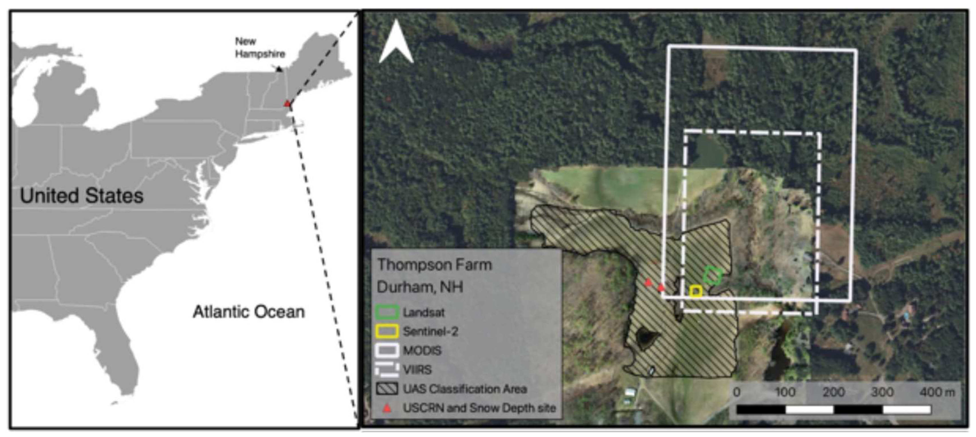
Figure 2.
UAS and satellite remote sensing product availability over the Thompson Farm study area for the period from January 24 to April 6, 2021.
Figure 2.
UAS and satellite remote sensing product availability over the Thompson Farm study area for the period from January 24 to April 6, 2021.
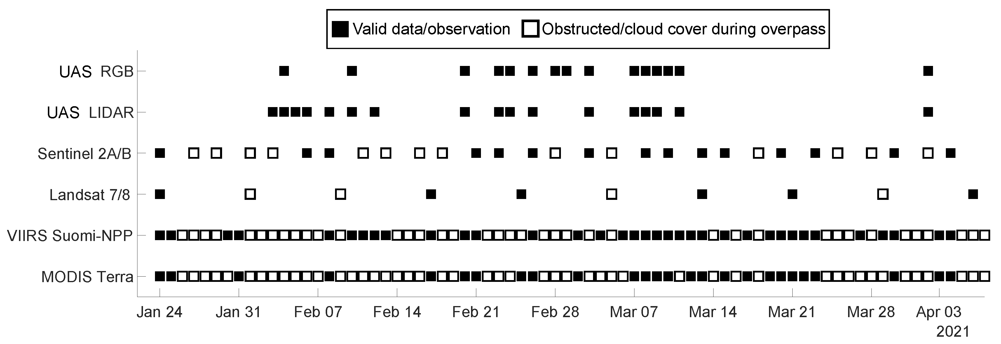
Figure 3.
UAS LiDAR-derived static spatial predictors (20 cm – 1 m pixel size) of snow cover over the Thompson Farm field with a histogram of the predictor’s distribution in the field (A–G). NDSImean (H) is the unscaled NDSI average for Sentinel-2 (20 m pixel size) using clear sky overpasses during the snow cover depletion period from February 23 – April 2, 2021.
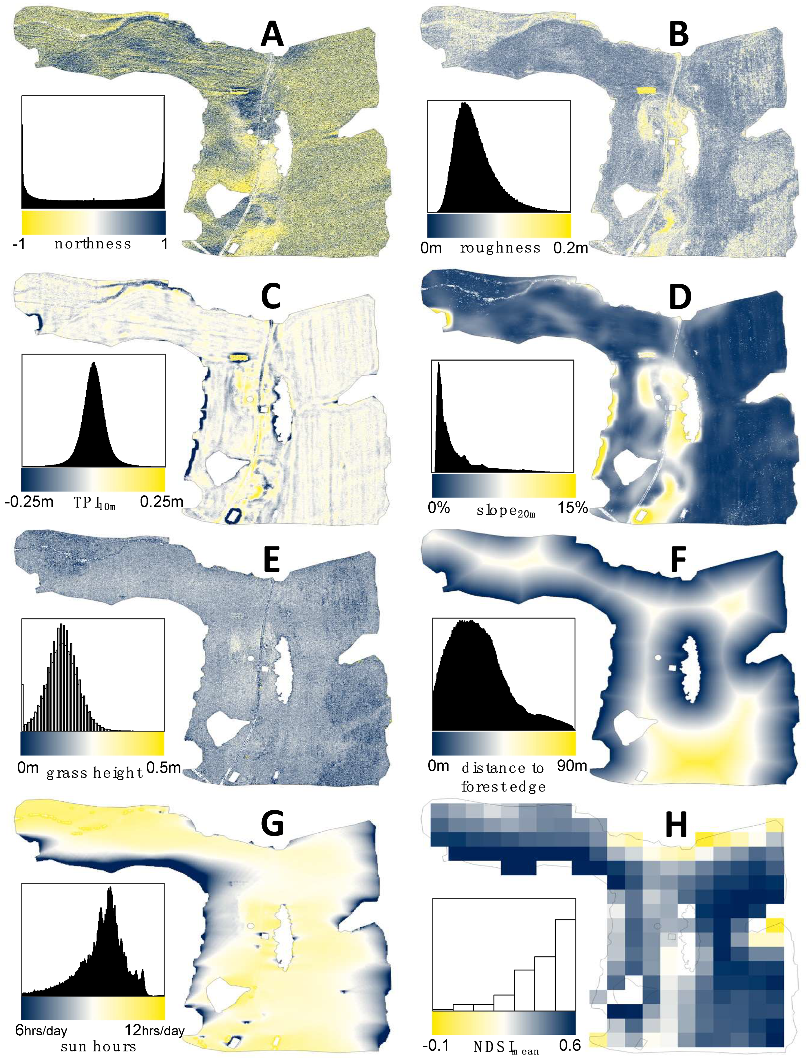
Figure 4.
Random forest (RF) modeling workflow for sub-meter resolution snow-covered area (SCA) estimation. Sentinel-2 Normalized Difference Snow Index (NDSI) is shown along with an NDSI to fractional SCA conversion function (NDSI-fSCA). Example shows observations and outputs from March 8, 2021, though the model was trained with all 6 days having both UAS and Sentinel-2 observations.
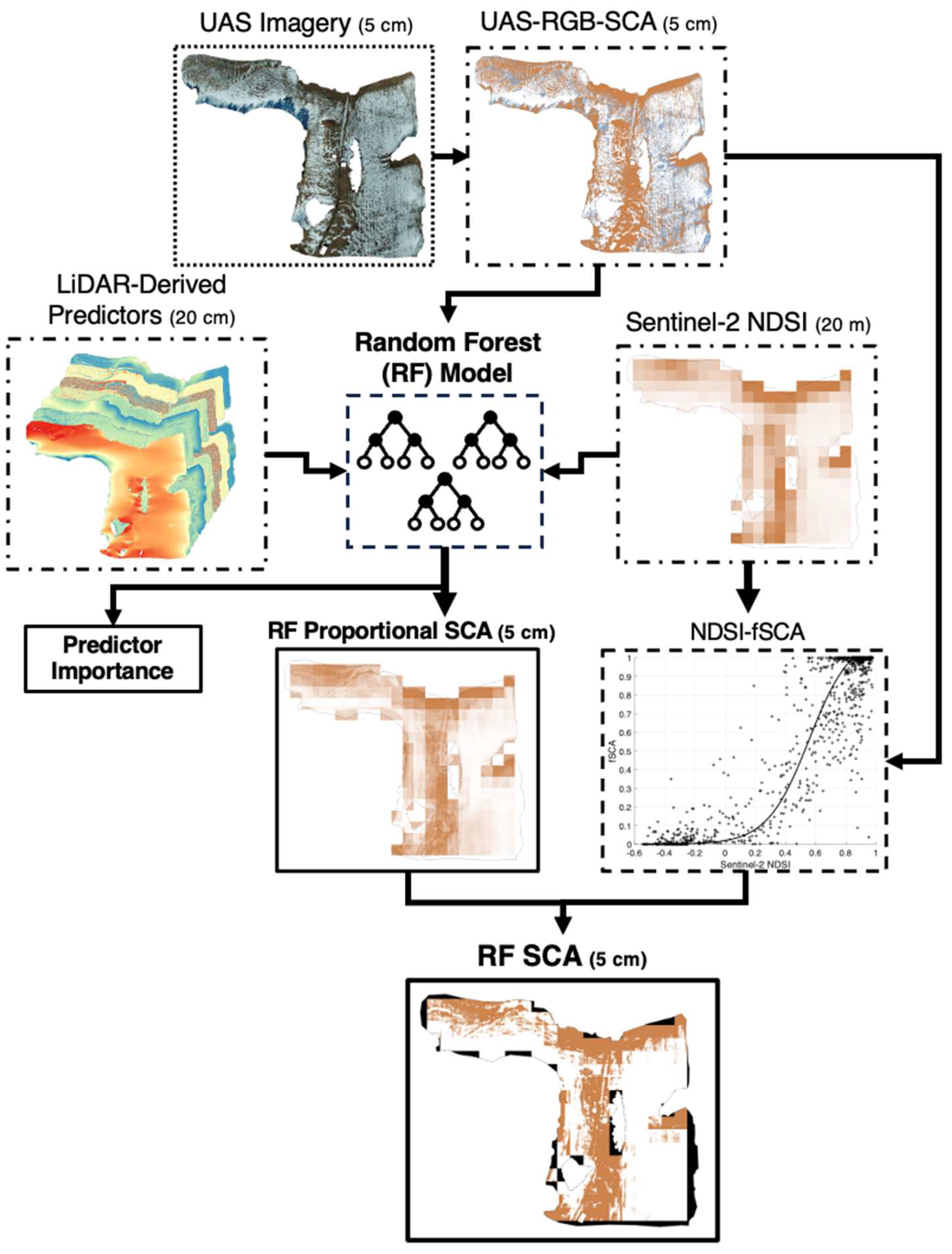
Figure 5.
Observed meteorologic conditions at the Thompson Farm USCRN site and snow depth stake. The top panel presents air temperature, soil temperature at 5 cm below the surface (daily averages), and solar radiation (hourly), while the bottom panel presents snow depth (from field cameras) and daily total precipitation (from USCRN).
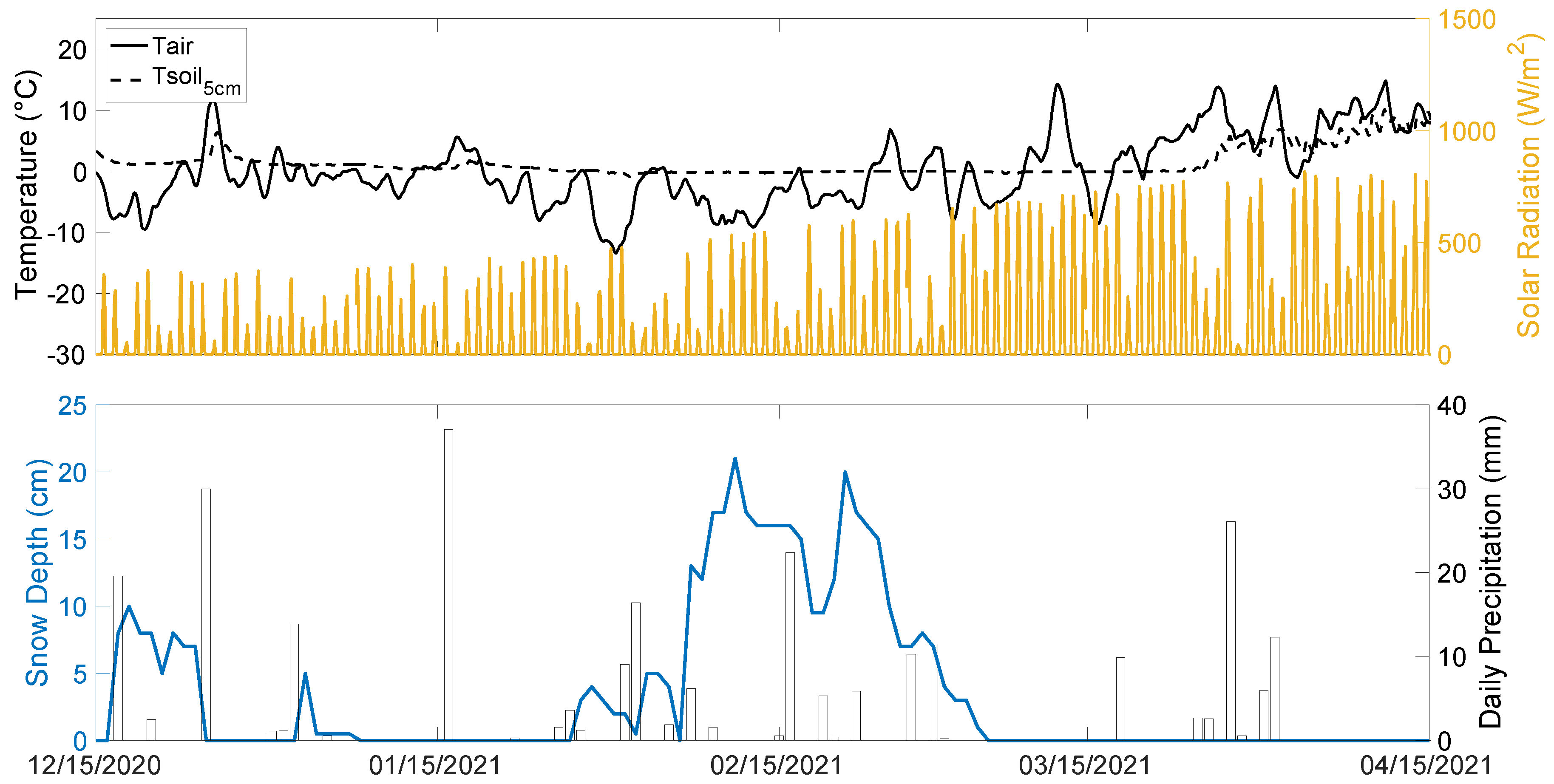
Figure 6.
UAS-RGB-SCA and manually delineated classes with test area results for select dates during the ablation period. From left to right; RGB orthomosaics from the UAS visible imagery, UAS-RGB-SCA classifications, and comparisons for each of the three test areas (blue, green, and red) by date. Test areas include the north site (blue box), central site (green box), and south site (red box). Test areas include zoomed RGB orthomosaics, UAS-RGB-SCA, and manually delineated classifications. Agreement between the latter two is also shown.
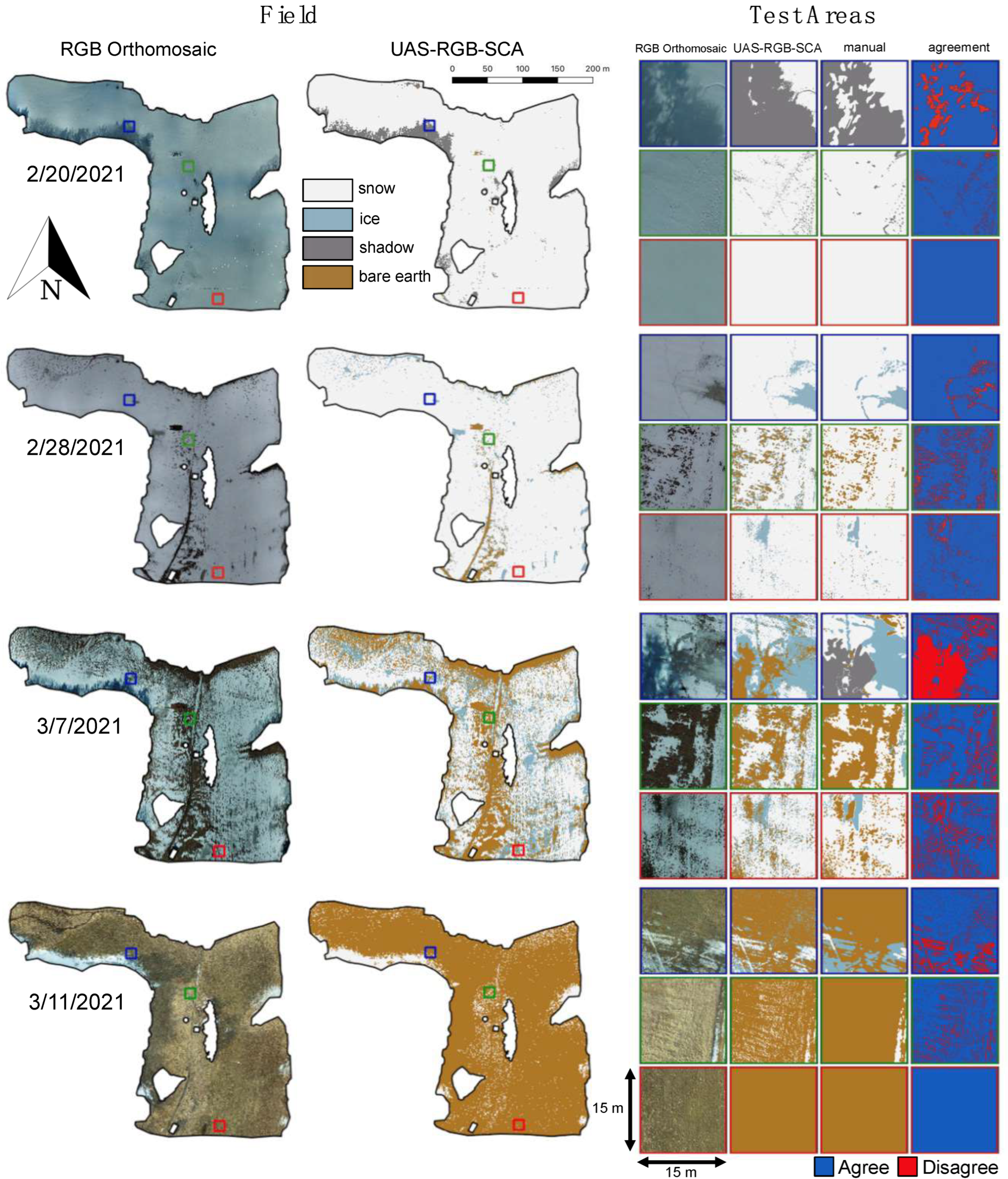
Figure 7.
UAS-RGB-SCA classifications considering all 15 flights from February 4 – April 2, 2021. Top maps illustrate the number of flights in which each pixel was classified as shadow (A) or ice (B). The lower panel shows snow persistence (C) as the ratio of the number of flights in which a pixel was classified as snow to the total number of snow or bare earth classifications.
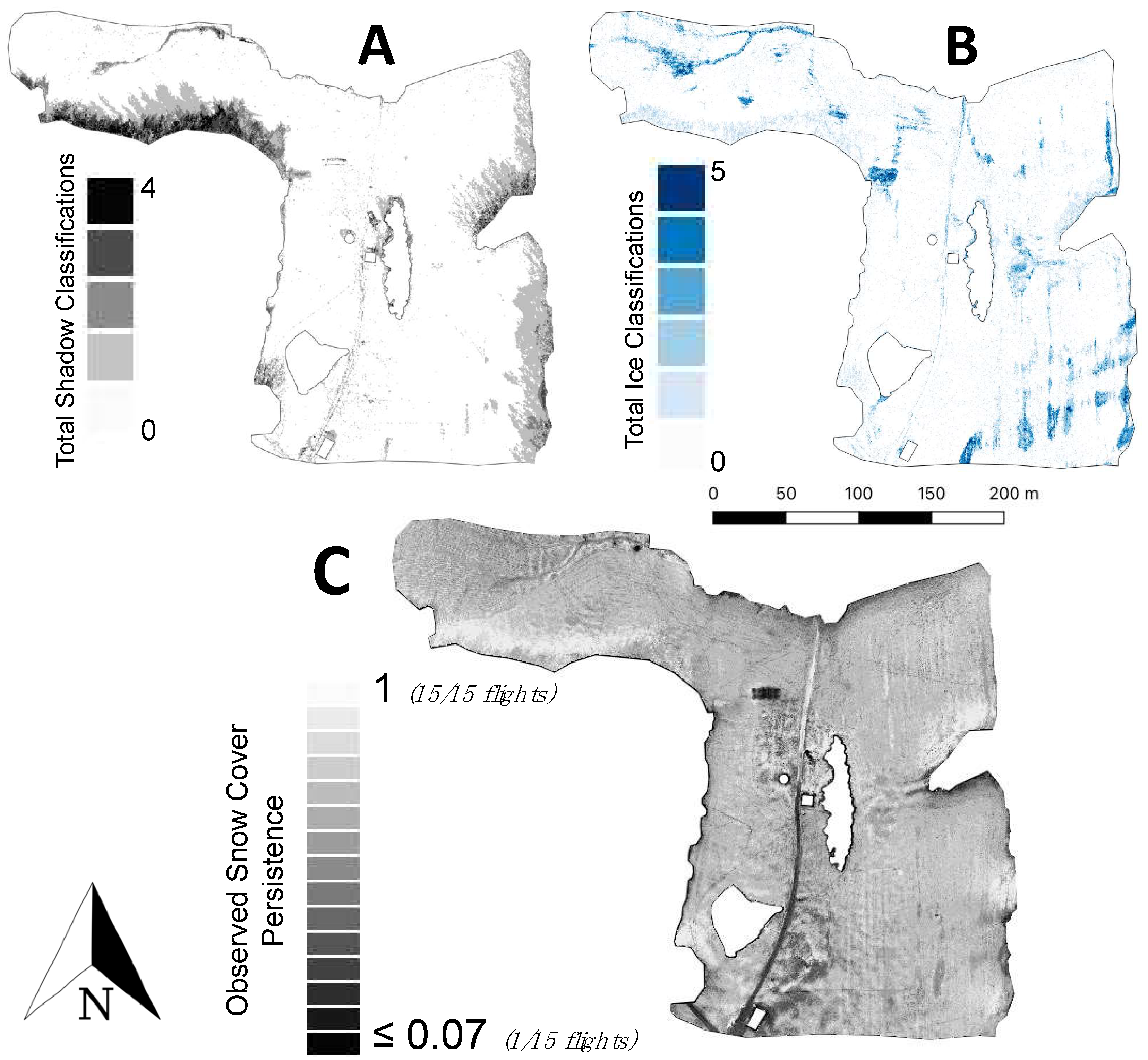
Figure 8.
Snow-covered area (SCA) observations summarized over the field site for UAS and satellite remote sensing products. Fractional SCA (fSCA) is computed as the field-wide snow cover proportion from the high-resolution UAS products (UAS-RGB-SCA and UAS-LiDAR-SCA) and weighted averages of pixels overlapping the study area for satellite products. NDSI values (blue) are normalized considering the range of the highest and lowest observed values for each product during the study period.
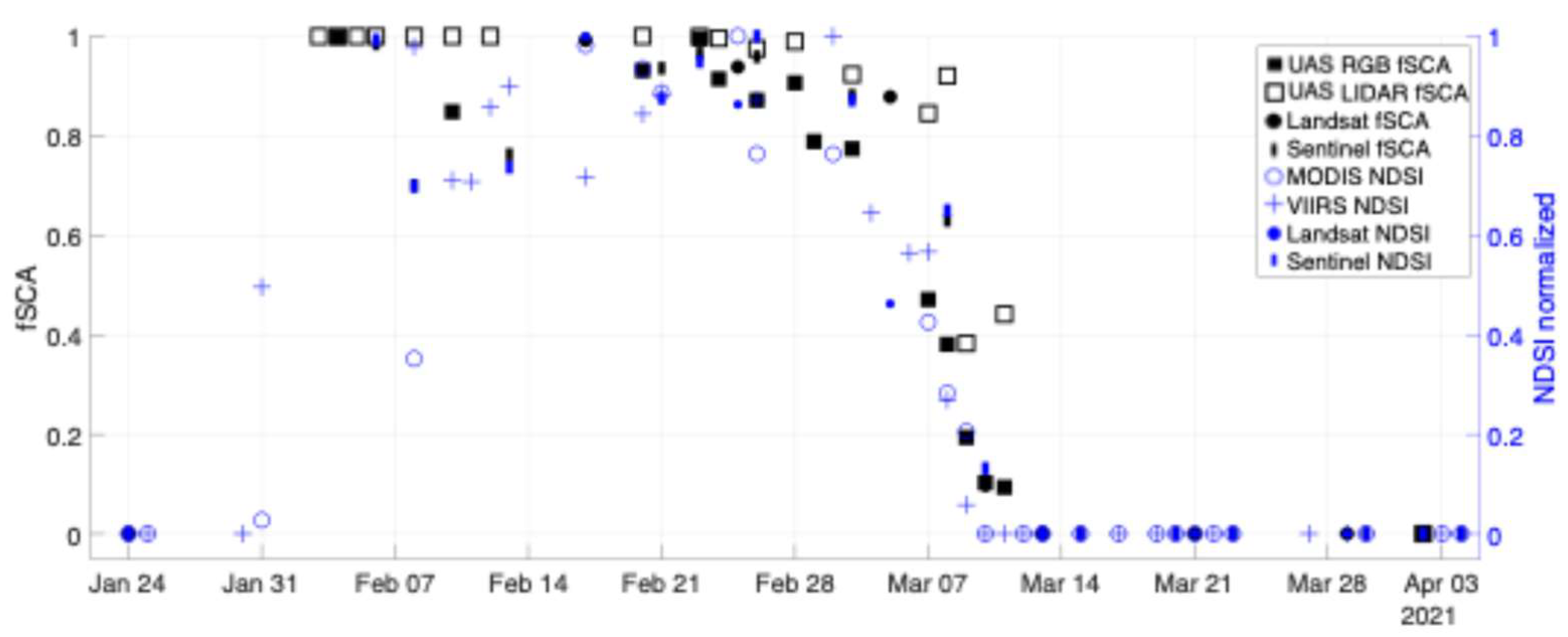
Figure 9.
Scatter plots and correlation value (R2) of field-wide fSCA calculated from the reference UAS-RGB-SCA snow cover product (x-axis) to field fSCA derived from UAS-LiDAR-SCA (A), UAS LiDAR field average snow depth (B), and satellite-derived fSCA and NDSI field weighted averages (C-H, y-axis). N = 15 for all days with UAS fSCA observations where solid points indicate that the product was observed on the same date and + points indicate non-UAS-RGB-SCA product was interpolated. Same date R2 values are shown first followed by the interpolated and same date data R2 values in parentheses.
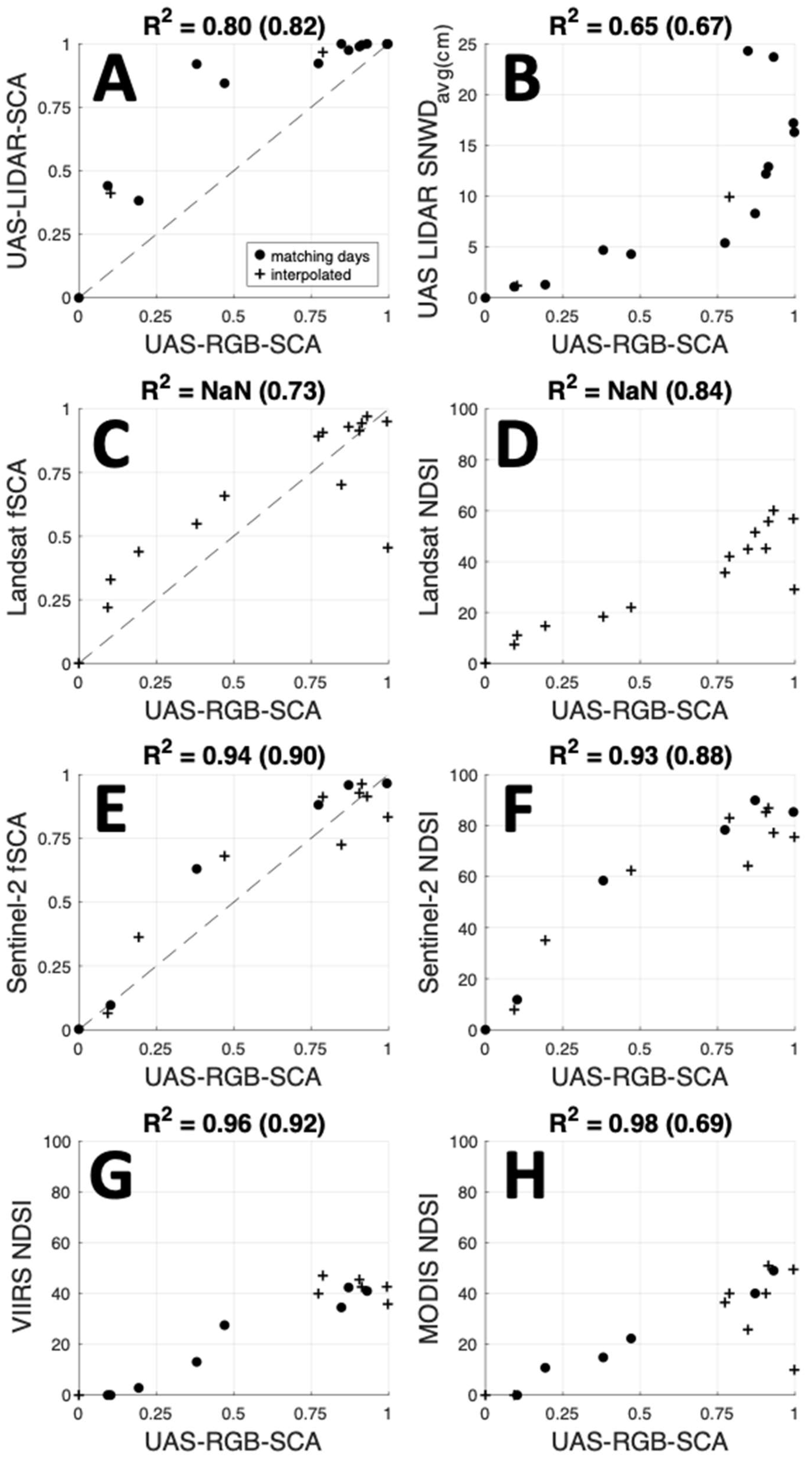
Figure 10.
Normalized predictor importance (permuted delta error) of snow-covered area from the trained random forest SCA (RF SCA) model.
Figure 10.
Normalized predictor importance (permuted delta error) of snow-covered area from the trained random forest SCA (RF SCA) model.
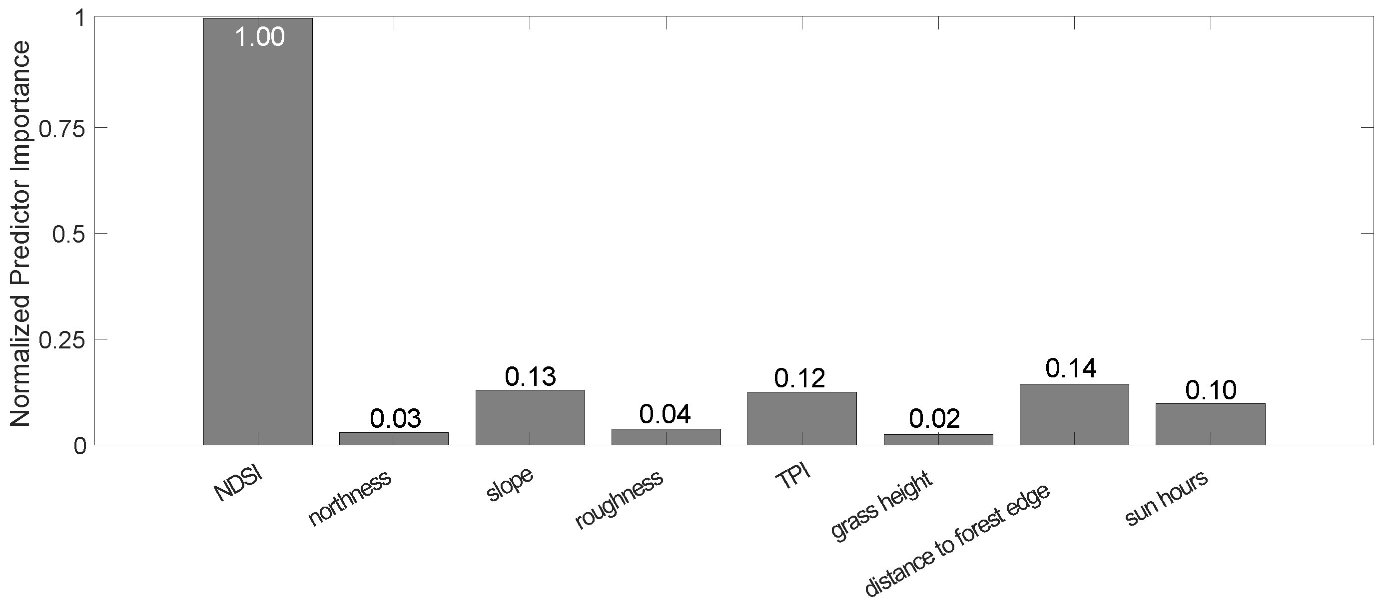
Figure 11.
UAS-RGB-SCA classifications, unscaled Sentinel-2 NDSI observations, RF Proportional SCA (the proportion of decision trees in the random forest predicting snow cover), and the RF SCA (from left to right columns) for dates with UAS collections and cloud-free Sentinel-2 observations.
Figure 11.
UAS-RGB-SCA classifications, unscaled Sentinel-2 NDSI observations, RF Proportional SCA (the proportion of decision trees in the random forest predicting snow cover), and the RF SCA (from left to right columns) for dates with UAS collections and cloud-free Sentinel-2 observations.
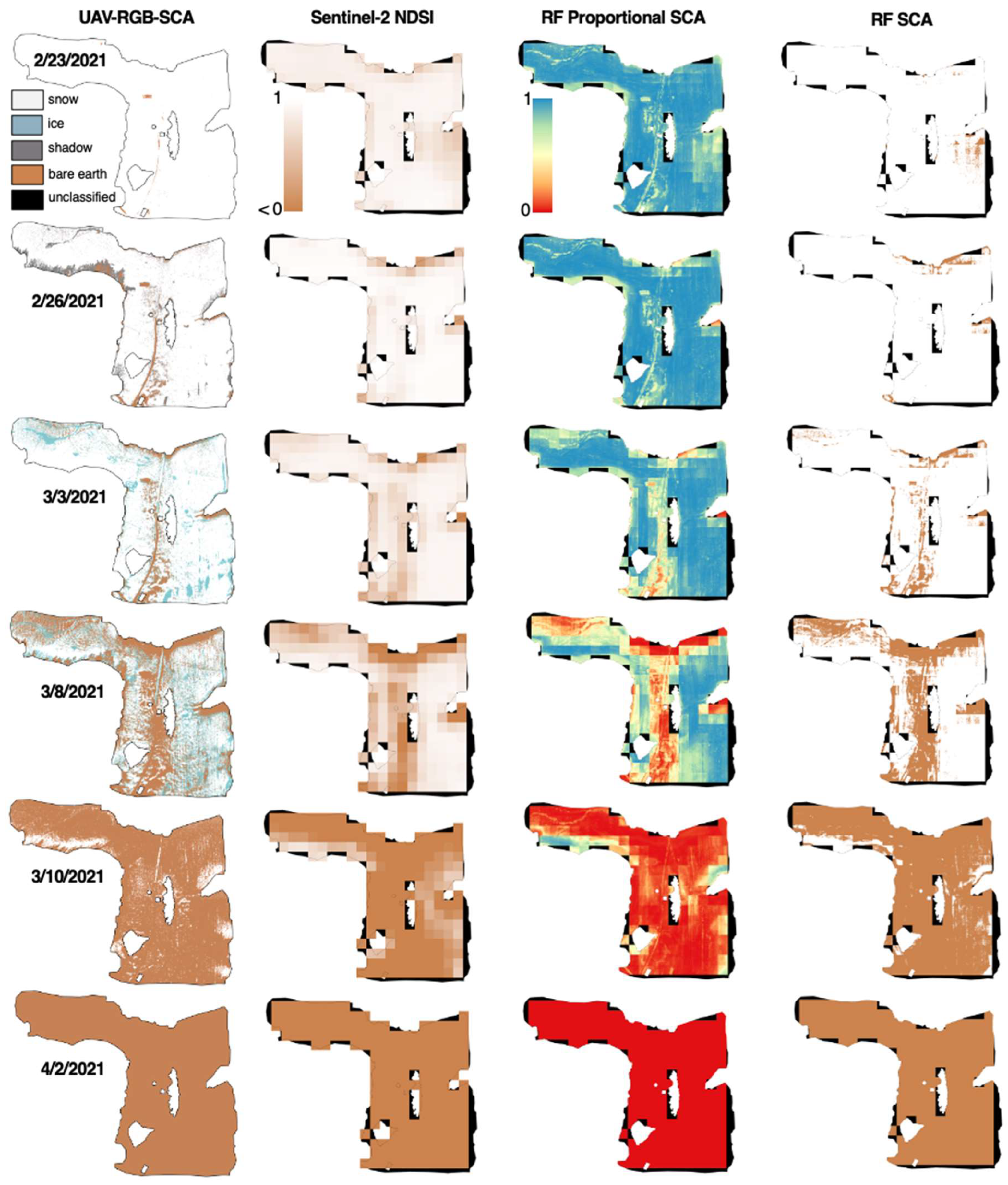

Table 1.
Overall accuracy and F1-score between UAS-RGB-SCA and manually delineated classes for 5 cm pixels) and the fractional snow-covered area (fSCA) by test area for select dates during the ablation period. For cover class where snow and bare earth do not add to 100%, the remaining area is shadow or ice (those with >10% shadow or ice are bolded). Complete summaries of UAS-RGB-SCA classifications (Table S1) and accuracy metrics (Table S2) are included in the accompanying Supplemental Material document.
| Date | Overall Accuracy | F1 score (snow) | Cover Class % snow (% bare earth) |
||||||
|---|---|---|---|---|---|---|---|---|---|
| North | Central | South | North | Central | South | North | Central | South | |
| 20-Feb-2021 | 89% | 97% | 100% | 0.85 | 0.99 | 1.00 | 36%(0%) | 97% (0%) | 100% (0%) |
| 24-Feb-2021 | 94% | 92% | 100% | 0.96 | 0.97 | 1.00 | 83%(0%) | 97% (0%) | 100% (0%) |
| 28-Feb-2021 | 96% | 87% | 95% | 0.98 | 0.96 | 0.98 | 91% (0%) | 84% (16%) | 94% (1%) |
| 3-Mar-2021 | 80% | 77% | 79% | 0.88 | 0.88 | 0.94 | 67%(4%) | 55% (39%) | 82%(6%) |
| 7-Mar-2021 | 33% | 83% | 56% | 0.80 | 0.77 | 0.71 | 33%(4%) | 36% (60%) | 75% (19%) |
| 11-Mar-2021 | 88% | 78% | 99% | 0.30 | 0.19 | -- | 2%(79%) | 4% (96%) | 0% (100%) |
| Mean | 80% | 86% | 88% | 0.80 | 0.79 | 0.93 | -- | -- | -- |
Table 2.
Fractional snow-covered areas (fSCA), bare patch (snow-off) counts, average bare patch area, and the associated fractal dimensions (Dp, Dk) for UAS-RGB-SCA and RF SCA snow cover products. Dp is the fractal dimension calculated from the relationship between the patch area-perimeter relationship and Dk is the fractal dimension calculated from Korcak’s law for estimating the size distribution of bare patches given their area. Bare patch analysis is not included for March 10 and April 2 due to minimal fSCA (< 0.10).
| Date | UAS-RGB-SCA | RF SCA | ||||||||
|---|---|---|---|---|---|---|---|---|---|---|
| fSCA (snow) |
Patch count | Mean patch area | Dp | Dk | fSCA | Patch count | Mean patch area | Dp | Dk | |
| 23-Feb-2021 | 1.00 | 2,278 | 0.19 m2 | 1.26 | 1.73 | 0.98 | 4,157 | 0.37 m2 | 1.31 | 1.61 |
| 26-Feb-2021 | 0.87 | 11,964 | 0.31 m2 | 1.24 | 1.70 | 0.96 | 1,515 | 1.46 m2 | 1.28 | 1.30 |
| 3-Mar-2021 | 0.77 | 29,310 | 0.29 m2 | 1.27 | 1.60 | 0.88 | 5,718 | 1.26 m2 | 1.30 | 1.41 |
| 8-Mar-2021 | 0.38 | 22,394 | 1.83 m2 | 1.40 | 1.55 | 0.65 | 7,554 | 3.72 m2 | 1.31 | 1.29 |
| Mean | 0.75 | 16,487 | 0.66 m2 | 1.29 | 1.64 | 0.87 | 4,736 | 1.70 m2 | 1.30 | 1.40 |
Table 3.
UAS-RGB-SCA classification (5 cm) by date and agreement of the UAS-RGB-SCA product with (1) binary classifications from Sentinel-2 and (2) the random forest modeled snow-covered area (RF SCA) where the UAS snow and ice classes were combined. The binary Sentinel-2 snow cover classification uses an NDSI threshold of 0.52 (i.e., fSCA value of 0.5).
| Date | UAS-RGB-SCA Class | Agreement with UAS-RGB-SCA Class | ||||||||
| Sentinel-2 | RF SCA | |||||||||
| snow | ice | shadow | bare earth | overall | UAS snow/ice | UAS bare earth | overall | UAS snow/ice | UAS bare earth | |
| 23-Feb-2021 | 99.5% | 0.0% | 0.0% | 0.5% | 97.1% | 97.6% | 3.1% | 97.8% | 98.3% | 1.0% |
| 26-Feb-2021 | 87.1% | 0.0% | 8.8% | 4.1% | 86.7% | 89.6% | 25.1% | 94.4% | 97.9% | 11.3% |
| 3-Mar-2021 | 77.4% | 13.9% | 0.0% | 8.7% | 82.6% | 87.4% | 32.7% | 90.5% | 94.6% | 46.7% |
| 8-Mar-2021 | 38.1% | 23.0% | 0.0% | 38.9% | 68.3% | 72.6% | 61.5% | 72.9% | 80.3% | 60.9% |
| 10-Mar-2021 | 10.3% | 0.0% | 0.0% | 89.7% | 89.5% | 27.4% | 96.6% | 89.0% | 41.3% | 94.0% |
| 2-Apr-2021 | 0.0% | 0.0% | 0.0% | 100.0% | 100.0% | -- | 100.0% | 100.0% | -- | 100.0% |
Disclaimer/Publisher’s Note: The statements, opinions and data contained in all publications are solely those of the individual author(s) and contributor(s) and not of MDPI and/or the editor(s). MDPI and/or the editor(s) disclaim responsibility for any injury to people or property resulting from any ideas, methods, instructions or products referred to in the content. |
© 2025 by the authors. Licensee MDPI, Basel, Switzerland. This article is an open access article distributed under the terms and conditions of the Creative Commons Attribution (CC BY) license (http://creativecommons.org/licenses/by/4.0/).
Copyright: This open access article is published under a Creative Commons CC BY 4.0 license, which permit the free download, distribution, and reuse, provided that the author and preprint are cited in any reuse.


