Submitted:
23 June 2025
Posted:
24 June 2025
You are already at the latest version
Abstract
Detecting surface water beneath vegetation canopies remains a major challenge for widely used water indices, which often underestimate water obscured by vegetation. This limitation is further compounded by the scarcity of reliable in-situ data needed for robust index development and validation. To address this, we introduce a Vegetation-Adjusted Water Index using a logarithmic transformation of the ratio between the Land Surface Water Index (LSWI) and the Enhanced Vegetation Index (EVI), referred to as VAWIlog. This transformation compresses high vegetation values while expanding the range typical of water surfaces, enhancing contrast in mixed land cover areas and improving class separability. The index was developed and validated using in-situ water level measurements, providing a strong empirical basis for detecting surface water under variable vegetation conditions. VAWIlog consistently outperformed established indices for detecting open water, wetlands, and flooded vegetation, demonstrating superior accuracy and overall detection performance. Evaluation against the Dynamic World V1 dataset confirmed its enhanced ability to identify water under vegetation, though some limitations remain in dense forest and open water contexts. Overall, VAWIlog offers a simple yet effective solution for improved surface water mapping in vegetated landscapes. Its compatibility with open-source optical satellite data supports broader applications in irrigation monitoring, and greenhouse gas assessments.
Keywords:
LSWI
; EVI
; vegetation
; surface water
; irrigation monitoring
; optical satellite
1. Introduction
Optical satellite remote sensing satellites (e.g. Landsat, Sentinel, and MODIS) have significantly advanced the monitoring of surface water at large spatial scales by providing consistent and accurate observations from space. This monitoring is typically achieved through the use of spectral band combinations derived from top-of-atmosphere or surface reflectance data. These combinations, commonly referred to as water indices, enhance the spectral contrast between water and non-water features, facilitating more accurate detection. Numerous water indices have been extensively employed to detect open surface water across a variety of environments, including lakes, reservoirs, and rivers [1,2,3]. One of the earliest and most widely used indices for surface water detection is the Normalized Difference Water Index (NDWI), which utilizes reflectance values from the near-infrared (NIR) and green spectral bands [4]. A modified version of NDWI was later introduced by [5], which replaces the NIR band with shortwave infrared (SWIR) reflectance to improve water delineation, particularly in urban areas characterized by complex land cover. Additional indices, such as, the Water Ratio Index (WRI) and the Automated Water Extraction Index (AWEI), have also been developed to address the challenges of detecting surface water in heterogeneous landscapes comprising of vegetation, built-up areas, and water bodies [6,7,8].
However, the detection of surface water beneath vegetation canopies remains a significant limitation of commonly used water indices. These indices often underestimate the presence of standing water obscured by vegetation, particularly in densely vegetated environments [9] In vegetative environments, optical remote sensing has primarily been applied to estimate canopy or vegetation water content, with a strong emphasis on drought monitoring and crop yield prediction [10,11,12]. In these applications, vegetation indices, such as, the Normalized Difference Vegetation Index (NDVI) are commonly used to assess vegetation health and density by exploiting the high reflectance of NIR band and the strong absorption of red band by healthy vegetation [13]. Similarly, the Enhanced Vegetation Index (EVI) has been developed to improve sensitivity to atmospheric conditions and reduce background noise, making it especially effective in regions with high biomass or cloud cover [14].
Nevertheless, there is a growing need to detect not only vegetation water content but also the presence or absence of surface water beneath vegetation, particularly to support irrigation management at both field and regional scales [15,16]. This need is also critical for accounting for greenhouse gas emissions resulting from prolonged flooding in agricultural systems such as paddy rice cultivation [17,18,19]. The Land Surface Water Index (LSWI) has been widely adopted in applications related to wetlands, irrigation monitoring, and drought assessment, owing to its sensitivity to both vegetation water content and soil moisture. It utilizes reflectance in the NIR and SWIR spectral regions [20,21,22]. LSWI, either on its own or in combination with EVI, has been extensively employed for mapping flooded rice paddies and estimating irrigation events [23,24,25,26]. But, its applicability in detecting surface water under vegetation continues to pose a challenge, as water indices often exhibit strong correlations with vegetation indices, complicating their interpretation and increasing the risk of misclassification [27,28,29].
Furthermore, progress in this domain is constrained by the limited availability of reliable in-situ data required for robust index development and validation. While satellite imagery, expert interpretation, and field surveys are commonly used for remote sensing validation [30,31,32], the presence of accurate and representative ground-based measurements remains essential for ensuring the credibility and applicability of remote sensing products, particularly in complex land cover conditions [33].
In response to these challenges, this study proposes a Vegetation-Adjusted Water Index (VAWI), developed through systematic exploration of different LSWI and EVI formulations with the objective of reducing the influence of vegetation on water detection, thereby enhancing the reliability of surface water identification under dense vegetative cover. A key innovation of this research is the integration of in-situ water level measurements which captures a wide range of water level variability both above and below the soil surface, collected throughout an entire rice cropping season. These measurements serve as ground truth for optimizing index thresholds and evaluating performance. Performance assessment includes a comparative analysis of the best-performing VAWI fomulation against standard indices used for open surface water and wetland monitoring, as well as an evaluation of index performance across varying vegetation density. This approach harnesses the synergy between satellite observations and field-based data to develop a modified water index tailored to improve surface water detection in rice paddies. Enhanced detection capabilities enabled by VAWI aim to extend the effective use of optical satellite data beyond early crop stages, thereby facilitating more accurate mapping of irrigation dynamics, supporting water balance assessments, and refining greenhouse gas emission estimates in paddy rice systems.
2. Data and Methods
2.1. On-the-Ground water Level Measurements
2.1.1. Sensor Installation
The field area for on-the-ground water level sensor installation is in Pangasinan, a province located in the northern Philippines. The Philippines predominantly follows a double-cropping system, characterized by distinct wet and dry seasons [34]. Wet season cropping typically occurs from June to October, while dry season cropping is generally from November to April [35]. The timing of transplanting and harvesting across the country varies depending on the availability of irrigation water, which continues to be a major challenge in agricultural management [36].
A total of 100 sensors were deployed during the dry season November 2024 to February 2025 across the study area, organized into three main clusters to ensure comprehensive spatial coverage and variability, as shown in Figure 1. The water level sensors are ultrasonic devices that measure water levels by emitting ultrasonic waves and calculating the time taken for the reflected waves to return. These sensors deliver precise readings every 15 to 16 minutes. Regular maintenance was performed to minimize potential errors and ensure measurement accuracy. This involved removing accumulated mud beneath the perforated pipe, clearing leaf debris, and guaranteeing that sensor measurements remained consistent with manual measurements across all sensors. Each sensor is mounted on a 30 cm PVC pipe, with 10 cm extending above the ground and 20 cm positioned below, capturing broad range of water level measurements. Water levels from the soil surface up to +10 cm are classified as indicative of water presence, while levels from the soil surface down to -20 cm are indicative of water absence. Thus, even if the soil appears moist when water levels are by the soil surface, it will still be considered indicative of water absence.
2.1.2. Time Series Smoothing and Dynamic Outlier Detection
Despite strict maintenance protocols, sensor malfunctions and obstructions, from leaves and other natural disturbances, can introduce outliers in the water level measurements. For data quality maintenance, a dynamic outlier detection algorithm using a sliding window is applied. For this process, a window size of n = 15 is selected to identify unnatural fluctuations in water levels. Regardless of factors like irrigation, rainfall, or drainage, water levels are expected to exhibit consistent rising or falling trend. By using a small window size, this approach conservatively removes outliers within a short time frame. The dynamic mean and standard deviation are computed for each time t using a 15-point centered window, as shown in Eq. (1) and (2):
represents the water level measurements at time t, and and denote the dynamic mean and standard deviation at time t, respectively, calculated within the sliding window. A measurement is identified as an outlier if its deviation from the dynamic mean exceeds twice the dynamic standard deviation. The water level measurement is retained only if it falls within an acceptable range, i.e., within two standard deviations from the dynamic mean. This process is summarized in Eq. (3):
Figure 2 presents three sample water level time series from selected fields, highlighting the detection and removal of significant outliers, from abrupt spikes or drops, attributed to sensor malfunctions or temporary obstructions. By applying a short time window to dynamically compute the local mean and standard deviation, the water level time series are effectively smoothed for more consistent data. The sample time series also showcases the distinct water level trends unique to each field, emphasizing the variability in hydrological patterns across different paddy fields.
2.2. Satellite Data
2.2.1. Data Pre-Processing
This study utilized surface reflectance data from the Harmonized Landsat and Sentinel-2 (HLS) project [37], which integrates imagery from the Landsat Operational Land Imager (OLI) and the Sentinel-2 MultiSpectral Instrument (MSI). The harmonized product maximizes the availability of optical satellite observations by combining the 16-day revisit cycle of Landsat with the 5-day revisit cycle of Sentinel-2 at the equator, enabling a more frequent and consistent monitoring of land surface conditions. Both sensors offer a spatial resolution of 30 meters, providing adequate detail for sub-field level analysis. The surface reflectance products used in this study are atmospherically corrected and preprocessed to reduce atmospheric noise, making them well-suited for time-series analysis and change detection applications [38,39]. Cloud and cloud shadow masking were performed using the FMask quality assurance (QA) bit flags embedded within the image collection. Following this pre-processing step, the Land Surface Water Index (LSWI) and Enhanced Vegetation Index (EVI) were calculated using their respective spectral band combinations, as defined in Eq. (4) and (5):
2.2.2. Temporal Alignment of Satellite and Water Level Data
Satellite data provides field information at regular intervals. With revisit frequency of at least five days, it is much less frequent than the 15–16-minute interval of water level measurements. As a result, satellite data serves as a practical basis for temporal alignment with the more frequent in-situ measurements. This process involves synchronizing the date and time of both datasets to a common time zone, in this case, Japan Standard Time (JST). While any time zone of choice is acceptable, making sure that both datasets adhere to the same time zone is necessary for maintaining consistency. Temporal alignment is achieved by identifying the closest date-time from the water level dataset to each satellite date-time, then associating the corresponding water level values with the satellite band values, as shown in Eq. 6:
where and represent the satellite and water level date-times, and and are the corresponding satellite and water level values. Finally, to account for potential installation errors and sensor sensitivity, data pairs with sensor readings between -1.0 cm and 1.0 cm were removed from the aligned dataset. Since a threshold of 0 cm is critical for determining water presence from water level measurements, even subtle errors in installation or sensor sensitivity could lead to misinterpretations of the satellite-derived results.
Figure 3a presents a time series boxplot of EVI throughout the dry season cropping period, at least for the field data collection locations. To provide context for the observed EVI values, key growth stages are also illustrated in Figure 3c, reflecting actual field conditions. These correspondences were verified with field staff on the ground. Figure 3b depicts data availability throughout the cropping season. The steady increase in data from mid-November to early December 2024 corresponds to the installation of water level sensors, coinciding with the completion of land preparation and the start of transplanting. From December to January 2025, data availability remains relatively stable. By late January 2025, fields that started activities earlier begin harvesting, leading to a gradual decline in available data. By early February, the remaining unharvested fields undergo terminal drainage in preparation for harvesting within the next one to two weeks, resulting in a reduction in water presence during this period.
A total of 682 aligned data points were obtained by temporally aligning satellite observations with water level measurements, comprising 218 instances of water presence and 464 instances of water absence. Water presence was observed throughout the season, confirming that controlled flooding is essential for rice growth and must be accurately captured. This flooding pattern indicates two possible scenarios: (1) some fields practice continuous flooding, while (2) others follow a rotational flooding schedule, where different groups of fields are alternately flooded and drained on different days.
2.3. Vegetation-Adjusted Water Index Formulations and Their Interpretations
The Vegetation-Adjusted Water Index (VAWI) is proposed to address the persistent challenge of detecting surface water beneath vegetative cover by minimizing the influence of vegetation. In this study, multiple vegetation correction transformations were formulated by combining LSWI and EVI in different mathematical structures. The corrected VAWI formulation represents a simple linear difference that reduces vegetation interference by subtracting the EVI from the LSWI. This operation lowers the values for vegetation-dominated pixels while preserving higher values for water, which typically has high LSWI and low EVI. The normalized difference form scales the difference between LSWI and EVI by their combined magnitude, accounting for overall signal intensity and reducing bias in mixed pixels. This enhances the contrast between water and vegetated surfaces. In the weighted formulation, the water signal (LSWI) is adjusted by the inverse of EVI. Since vegetation has high EVI, the resulting weight becomes small, suppressing the signal in vegetated areas. For water bodies with low EVI, the weight remains high, preserving the original LSWI. This non-linear scaling effectively reduces vegetation influence. The normalized vegetation-adjusted form modifies the LSWI–EVI difference based on vegetation dominance. When EVI is high, the adjustment reduces the index value, while for low EVI, the formula amplifies the water signal. This enhances responsiveness to vegetation presence. Finally, the log-transformed variant applies a logarithmic transformation to the moisture-to-vegetation ratio. This compresses high vegetation values and expands low values typical of water surfaces, improving contrast in areas with subtle differences and making class separation more symmetric and linear.
A simple grid search optimization is employed to identify the optimal threshold for each vegetation-adjusted water index transformation. Five hundred (500) equally spaced candidate thresholds are generated based on the minimum and maximum values of each index. These thresholds are then individually assessed to determine their performance. Balanced accuracy is used as the optimization criterion, and the threshold that yields the highest balanced accuracy is selected as the optimal threshold. These candidate formulations were systematically evaluated based on a set of performance metrics described in Appendix A. The transformation that demonstrated the highest overall performance, as summarized in Table 1, is recommended as the VAWI.
3. Results and Discussion
3.1. Vegetation Influence Reduction and Performance of LSWI–EVI Transformations
With the primary objective of minimizing vegetation influence, Figure 4 presents the distribution of index values from each transformation plotted against vegetation density, as indicated by EVI. The baseline plot of LSWI against EVI reveals a positive correlation, indicating that LSWI values tend to increase with increasing vegetation density. All transformations demonstrate significant reductions in this correlation, evidenced by the decreased slopes of their trendlines, except for VAWINorm. Although VAWINorm reverses the correlation direction to negative, it does not exhibit a meaningful improvement in independence. This negative trend is likely due to the subtraction of EVI in both the numerator and denominator of its formulation, causing index values to decrease as vegetation increases. VAWIlog stands out among the tested transformations, exhibiting a near-zero slope and a nearly horizontal trendline, suggesting effective decoupling from vegetation influence.
The five LSWI–EVI transformation candidates exhibited varying levels of performance, as evaluated using balanced accuracy (BA), producer’s accuracy (PA), and user’s accuracy (UA). These metrics respectively reflect the overall classification effectiveness, the accuracy in detecting surface water under vegetation, and the reliability of detections, as illustrated in Figure 5. Among the transformations, VAWIlog achieved the highest balanced accuracy and producer’s accuracy, with BA = 0.69 and PA = 0.80, while also demonstrating a comparable user’s accuracy (UA = 0.47). A close second was VAWIcorrected, which yielded a BA of 0.68, PA of 0.73, and a slightly higher UA of 0.49.
Figure 4, particularly the distribution of labeled surface water presence and absence points, illustrates the rationale behind the formulation of VAWIlog. This index effectively reduces the influence of vegetation, thereby improving the separability between surface water presence and absence classes under vegetated conditions. This visual evidence supports the superior performance observed for this index. Moreover, Figure 4 and Figure 5 reveal a clear relationship between the slope of the index distribution trendline, representing the degree of vegetation influence, and the producer’s accuracy in detecting surface water beneath vegetation. Indices with flatter slopes indicate reduced sensitivity to vegetation density and tend to perform better in surface water detection. In particular, VAWIlog, which exhibited the flattest slope, achieved the highest producer’s accuracy, followed by VAWIweighted (PA = 0.77) and VAWIcorrected. In contrast, VAWINorm, which reversed the correlation but showed limited improvement in vegetation suppression, recorded the lowest detection accuracy (PA = 0.60).
Demonstrating superior performance and stability across increasing vegetation cover, VAWIlog emerged as the most effective transformation among the five LSWI–EVI variants evaluated.
3.2. Benchmarking Against Established Water Indices
Several water indices have been developed to detect the presence of surface water resulting from natural flooding or irrigation, primarily by capturing variations in surface wetness. Among these, the Normalized Difference Water Index (NDWI) and the Land Surface Water Index (LSWI) are widely used [25,40,41]. However, their effectiveness is often limited to early crop growth stages, when vegetation cover is minimal. The Normalized Difference Flood Index (NDFI), which combines red and SWIR2 reflectance bands, has been applied to estimate surface water in Italian rice-growing regions [42]. Its performance significantly declines with increasing vegetation density and vigor. In contrast, the Water in Wetlands (WIW) index was specifically designed to detect surface water in wetland environments, including vegetated areas such as forests, rice paddies, and shrublands, regardless of vegetation presence or absence [43]. In this section, we evaluate the performance of VAWIlog in comparison to several well-established water indices, focusing on both overall detection accuracy and robustness under increasing EVI.
3.2.1. Overall Detection Performance
Figure 6 presents the performance scores of VAWIlog alongside NDWI, LSWI, WIW, and NDFI, evaluated against ground truth observations. All these conventional indices demonstrated suboptimal performance, with balanced accuracy (BA) scores ranging only from 0.54 to 0.56. For NDWI, WIW, and NDFI, this lower performance primarily stems from their limited ability to detect surface water under vegetation cover. In contrast, LSWI exhibited strong producer’s accuracy (PA), indicating effective detection of surface water presence; however, its low user’s accuracy (UA = 0.35) suggests considerable overestimation. VAWIlog, while achieving similarly high PA to LSWI, significantly improved UA due to reduced vegetation influence. This enhancement resulted in a more reliable prediction and a substantial increase in overall detection performance.
Figure 7 presents box plots of NDWI, LSWI, NDFI, and VAWIlog values under surface water presence and absence conditions. WIW is excluded from this comparison because it is based on direct thresholding of NIR and SWIR reflectance and does not produce continuous values. The distributions indicate substantial overlap between presence and absence classes for NDWI, LSWI, and NDFI, highlighting their limited discriminative ability under complex surface conditions. In contrast, VAWIlog shows a more distinct separation, with higher values consistently associated with surface water presence and lower values with its absence. This suggests that the logarithmic transformation of the LSWI–EVI ratio improves class separability, particularly in mixed or vegetation-covered areas where traditional indices tend to underperform.
3.2.2. Detection Stability with Increasing EVI
Evaluating the performance of VAWIlog under varying vegetation conditions is essential to demonstrate its effectiveness and consistency, especially in areas with dense crop cover. Figure 8a and 8b show the Balanced Accuracy (BA) and Producer’s Accuracy (PA), respectively, for NDWI, LSWI, WIW, NDFI, and VAWIlog across increasing vegetation density (EVI). Figure 8c presents the number of surface water presence and absence instances per EVI range, confirming that surface water remains present even at high vegetation densities, highlighting the need for reliable detection beyond early crop stages.
Figure 8a shows that VAWIlog consistently outperforms all other indices across the entire range of EVI values, demonstrating superior detection capabilities regardless of vegetation density. While LSWI shows competitive performance at low to moderate vegetation levels, its accuracy declines at both ends of the spectrum, whereas VAWIlog maintains high detection performance throughout. Further insights into the limitations of each index are provided in Figure 8b. NDWI, WIW, and NDFI perform reasonably well under low EVI conditions, corresponding to early growth stages shortly after transplanting. However, their detection capabilities decline rapidly beyond EVI = 0.2 and become ineffective (PA ≈ 0) beyond EVI = 0.41, as vegetation becomes denser and begins to obscure surface water. LSWI shows increasing PA with higher vegetation cover, but this trend is potentially misleading. Its strong correlation with EVI suggests that elevated detection rates at high vegetation densities may stem from overestimation, as the index conflates vegetation moisture with surface water. In contrast, VAWIlog stands out for its consistent and accurate detection across all vegetation levels, effectively distinguishing surface water without being confounded by vegetation influence.
These findings are reinforced by the surface water presence probability heatmaps shown in Figure 9, which are derived using the optimal threshold for each index and validated against ground-based observations. NDWI, LSWI, and NDFI fail to provide clear separability between surface water presence and absence across varying vegetation conditions while, VAWIlog maintains strong separability throughout, demonstrating its reliability and suitability for detecting surface water under vegetated environments.
3.3. Benchmarking Against Dynamic World V1 Dataset
Dynamic World V1 is a near-real-time (NRT) dataset that classifies Sentinel-2 imagery into eight distinct land use/land cover (LULC) classes: water, trees, grass, flooded vegetation, crops, shrubs and scrub, built-up areas, bare ground, and snow and ice [30]. The dataset is developed using semi-supervised learning based on expert-labeled samples. Specifically, the "flooded vegetation" class is annotated only when there is a clear visual intermixing of water and vegetation, such as emergent vegetation where surface water remains visible in the satellite imagery. Consequently, the Dynamic World training data for this class primarily represents low-density or sparse vegetation conditions, typically associated with low EVI values.
To assess Dynamic World’s capability in detecting surface water within vegetated agricultural areas, we compare its land cover classifications with in-situ water level measurements across the study period. All monitored fields are confirmed rice-growing areas, where correct classifications should predominantly fall under either "crops" or "flooded vegetation." As shown in Figure 10a, 80.5% of observations are labeled as crops, while only 3.0% are classified as flooded vegetation. Misclassifications occur, with some fields incorrectly labeled as trees (8.8%) or built-up areas (2.5%). For performance evaluation, Figure 10b simplifies the classification scheme into binary categories: surface water presence (water and flooded vegetation) and absence (all other classes). This enables a direct comparison with both sensor-based measurements and VAWIlog performance.
The performance comparison, in Figure 11 highlights the significant limitations of Dynamic World dataset. Dynamic World achieves a BA of only 0.53, largely due to its severe underestimation of flooded vegetation, reflected in a low detection accuracy (PA) of just 0.11. This indicates that the datasets detects surface water presence in vegetated areas only 11% of the time. This shortcoming aligns with the nature of the training data preparation, where "flooded vegetation" is labeled only when water is visibly discernible, typically under sparse vegetation conditions. As such, Dynamic World may be of limited use beyond the early stages of the rice-growing season, such as during land preparation or transplanting, when vegetation cover is minimal. In contrast, VAWIlog demonstrates better performance, owing to its development in conjunction with ground-based water level measurements. This synergy between satellite observations and in-situ data enables VAWIlog to capture surface water dynamics more reliably, even under dense vegetation. The results underscore the value of integrating remote sensing with field observations to develop indices that outperform conventional water detection methods and datasets.
3.4. In Developing Surface Water Maps
The capabilities of VAWIlog in developing a high-resolution and accurate general surface water maps are compared against NDWI and Dynamic World V1 near-real time (NRT). Figure 12 presents surface water maps for an area in Pangasinan, Philippines, across two acquisition dates. The first panels show the EVI map, showing the variable vegetation conditions (e.g. no, sparse, moderate and dense) that influence water visibility. The second panels display the Dynamic World V1 land cover classification, used for visual reference. The third and fourth panels show surface water segmentation results derived from VAWIlog and NDWI, respectively. These maps cover a broad area encompassing diverse land cover types to demonstrate the consistency of surface water detection across different landscapes and seasonal conditions.
For open surface water types, particularly rivers and reservoirs, VAWIlog exhibited a tendency to underestimate surface water extent. This limitation may be attributed to its LSWI-based formulation, where the low reflectance of NIR in open water bodies can reduce the index’s sensitivity. Since LSWI relies on the difference between NIR and SWIR, its effectiveness can be diminished in detecting pure open water, where both NIR and SWIR reflectance values are typically very low, leading to weak contrast [4,44]. Thus, NDWI, which leverages strong water absorption in the green band and low reflectance in the NIR, demonstrated better performance in detecting open surface water bodies.
In forested areas, VAWIlog tends to overestimate the presence of surface water, whereas NDWI more effectively avoids false detections in these regions. This overestimation is likely due to inflated LSWI values in dense vegetation canopies, where the NIR reflectance remains relatively high and the SWIR reflectance can be suppressed by internal canopy moisture or shadows, misleadingly mimicking surface wetness. Since VAWIlog has so far been validated primarily in low-stature vegetation environments such as rice paddies, its applicability in complex, mixed vegetation landscapes, including forests, wetlands, and tree-covered floodplains, warrants further investigation.
In areas with flooded vegetation and croplands, VAWIlog shows strong agreement with the flooded vegetation class in Dynamic World V1 especially during 2025-01-21 capture data in Figure 12a. In contrast, NDWI significantly underestimates the extent of flooding in these vegetated regions. Notably, VAWIlog also identifies additional flooded areas, particularly within the croplands on the right side of the image, which are not captured by Dynamic World.
Consequently, Dynamic World’s flooded vegetation detection is likely accurate only under conditions of low vegetation cover. As vegetation density increases, particularly in areas with moderate to dense vegetation, as in Figure 12b, Dynamic World tends to miss flooded regions that VAWIlog is able to detect. This highlights the enhanced capability of VAWIlog to capture surface water beneath vegetation, even in comparison to a semi-supervised product like Dynamic World. Supporting this, [45] reported that Dynamic World has difficulty detecting flooded vegetation, with class-specific accuracies as low as 53%, underscoring the limitations of such datasets in complex, vegetated environments.
For additional context, rice farmers in the region typically follow two main cropping seasons: one during the dry season and another during the wet season. However, in areas with reliable water access—particularly fields located near reservoirs or dams—a third cropping cycle is sometimes feasible. In such cases, farmers may adjust their schedules, initiating the dry season earlier than usual to accommodate a second dry-season crop before the onset of the wet season. Among the study sites, fields designated for general data collection adhere to the conventional two-season cropping pattern. In contrast, the location selected for the surface water mapping demonstration benefits from proximity to a major water source, allowing for third-cropping practices. The image captured on 2025-01-21 corresponds to the early stage of this third cropping cycle, with the fields advancing toward the maturity phase by the time of the 2025-02-20 acquisition.
Building on the observed behavior of VAWIlog and NDWI across various land cover types, we propose a combined approach that integrates VAWIlog, NDWI, and Dynamic World V1 to generate comprehensive surface water maps. In this framework, NDWI is used to detect open water and water beneath tree canopies as identified by Dynamic World V1, while VAWIlog is applied to other land cover classes such as crops, flooded vegetation, and shrubs. A demonstration of this integrated method is presented in Figure 10 using the two observation dates (a) 2025-01-21, and (b) 2025-02-25.
4. Conclusions
This study systematically explored various transformations of the LSWI-EVI relationship with the primary objective of reducing the influence of vegetation on surface water detection. Among all the transformations tested, the logarithmic transformation of the LSWI-to-EVI ratio, referred to as VAWIlog, emerged as the most effective. It consistently demonstrated the highest overall performance and detection accuracy, largely due to its ability to suppress vegetation interference while enhancing the separation between water and vegetative signals.
VAWIlog was then benchmarked against several widely used water indices designed for mapping open surface water, flooded vegetation, and wetlands. Across these diverse water conditions, VAWIlog consistently outperformed the other indices, not only in terms of overall detection accuracy, but also in maintaining stable performance across increasing vegetation density. Furthermore, when compared to the publicly available Dynamic World V1 dataset, VAWIlog demonstrates superior performance in detecting flooded vegetation. Notably, it identifies water presence in areas where Dynamic World fails to do so, underscoring its enhanced sensitivity to water bodies obscured by vegetation. This contrast highlights the advantages of developing indices in conjunction with in-situ water level measurements, rather than relying solely on expert annotation. This is particularly relevant in vegetated environments, where surface water can be partially or entirely obscured by canopy cover, making visual labeling less reliable.
However, the analysis also reveals certain limitations of VAWIlog. The index tends to underestimate open surface water, likely due to the influence of near-infrared (NIR) reflectance in its formulation, and may overestimate water presence in densely forested or heavily vegetated areas. Consequently, its optimal application is in low-vegetation environments such as rice paddies and wetlands, where it more accurately captures surface water dynamics. To achieve more comprehensive surface water mapping, encompassing reservoirs, lakes, rivers, and flooded vegetation, a combined use of VAWIlog and traditional water indices such as NDWI is recommended.
Through rigorous benchmarking against both conventional indices and global datasets, VAWIlog has established itself as a highly effective tool for detecting surface water under low to moderate vegetation cover. Its simplicity and compatibility with high-spatial and high-temporal open-source satellite data make it a practical option for improved irrigation monitoring and, ultimately, for estimating greenhouse gas emissions under different water management practice.
Author Contributions
Conceptualization, A.D., S.K.; methodology, A.D.; validation, A.D.; formal analysis, A.D.; investigation, A.D.; resources, A.D., S.K. and Z.B.; data curation, A.D. and Z.B.; writing—original draft preparation, A.D.; writing—review and editing, A.D. and S.K.; visualization, A.D.; supervision, S.K. and Z.B.; project administration, S.K.; funding acquisition, S.K. All authors have read and agreed to the published version of the manuscript.
Funding
This work was supported by JSPS KAKENHI Grant Number JP23K26203.
Data Availability Statement
Raw satellite images from Harmonized Landsat and Sentinel-2 (HLS) surface reflectance dataset and Dynamic World V1 LULC classification are all accessible in the Google Earth Engine plat-form.
Acknowledgments
The authors would like to express their sincerest gratitude to the anonymous reviewers, in advance. The authors would also like to acknowledge Mr. Mc Rayson Florendo for his dedicated efforts in maintaining the on-ground water level sensors, and Creattura Co. Ltd. for their trust and support in providing the water level measurements used in this study. During the preparation of this manuscript, the authors used ChatGPT 4 for the purposes of enhancing writing quality. The authors have reviewed and edited the output and take full responsibility for the content of this publication.
Conflicts of Interest
The authors declare no conflict of interest.
Appendix A
Appendix A.1. Performance Metrics
Given the following parameters:
- represents the instances where the water indices correctly predicted water presence (true positive).
- represents the instances where the water indices correctly predicted water absence (true negative).
- represents the instances where the water indices predicted water presence, but water was absent (false positive).
- represents the instances where the water indices predicted water absence, but water was present (false negative).
In the aligned dataset, 32% of the instances correspond to water presence, while 68% correspond to water absence. To address the class imbalance, balanced accuracy (BA) will serve as the primary metric for overall performance evaluation of the water indices. Balanced accuracy ensures equal weight is given to both water presence and absence, preventing skewed performance due to the overrepresentation of the absence class. This metric helps avoid misleading results that can arise from high overall accuracy when one class dominates, as shown in Eq. A1:
Supporting metrics will primarily assess the index’s ability to detect water beneath vegetation. The first key metric is Producer’s Accuracy (PA), which measures how effectively the indices detect standing water in all instances where it is present. PA is calculated using Eq. A2:
Another key supporting metric is User’s Accuracy (UA), which measures the pro-portion of correctly detected standing water among all instances classified as water presence. This metric assesses the reliability of both the index and the chosen threshold. UA is computed using Eq. A3:
During index thresholding, setting a very low threshold may artificially inflate Producer’s Accuracy (PA), but this comes at the cost of User’s Accuracy (UA), reducing the reliability of standing water detection. Therefore, the optimal index is one that maintains a balanced trade-off among PA, UA, and BA, ensuring accuracy, sensitivity and reliability.
References
- Jiang, W.; Ni, Y.; Pang, Z.; Li, X.; Ju, H.; He, G.; Lv, J.; Yang, K.; Fu, J.; Qin, X. An Effective Water Body Extraction Method with New Water Index for Sentinel-2 Imagery. Water 2021, 13, 1647. [Google Scholar] [CrossRef]
- Kwang, C.; Jnr, E.M.O.; Amoah, A.S. Comparing of Landsat 8 and Sentinel 2A using Water Extraction Indexes over Volta River. Journal of Geography and Geology 2017, 10, 1. [Google Scholar] [CrossRef]
- Nsubuga, F.W.N.; Botai, J.O.; Olwoch, J.M.; Rautenbach, C.; Kalumba, A.M.; Tsela, P.; Adeola, A.M.; Sentongo, A.A.; Mearns, K.F. Detecting changes in surface water area of Lake Kyoga sub-basin using remotely sensed imagery in a changing climate. Theoretical and Applied Climatology 2017, 127, 327–337. [Google Scholar] [CrossRef]
- McFEETERS, S.K. The use of the Normalized Difference Water Index (NDWI) in the delineation of open water features. International Journal of Remote Sensing 1996, 17, 1425–1432. [Google Scholar] [CrossRef]
- Xu, H. Modification of normalised difference water index (NDWI) to enhance open water features in remotely sensed imagery. International Journal of Remote Sensing 2006, 27, 3025–3033. [Google Scholar] [CrossRef]
- Kareem, H.; Attaee, M.; Omran, A. Estimation the Water Ratio Index (WRI) and Automated Water Extraction Index (AWEI) of Bath in The United Kingdom Using Remote Sensing Technology of The Multispectral Data of Landsat 8-Oli. Water Conserv. Manag 2024, 8, 125–132. [Google Scholar] [CrossRef]
- Rokni, K.; Ahmad, A.; Selamat, A.; Hazini, S. Water Feature Extraction and Change Detection Using Multitemporal Landsat Imagery. Remote Sensing 2014, 6, 4173–4189. [Google Scholar] [CrossRef]
- Shen, L.; Li, C. Water body extraction from Landsat ETM+ imagery using adaboost algorithm. In Proceedings of the 2010 18th International Conference on Geoinformatics. IEEE; 6 2010; pp. 1–4. [Google Scholar] [CrossRef]
- Declaro, A.; Kanae, S. Enhancing Surface Water Monitoring through Multi-Satellite Data-Fusion of Landsat-8/9, Sentinel-2, and Sentinel-1 SAR. Remote Sensing 2024, 16, 3329. [Google Scholar] [CrossRef]
- Zhang, J.; Xu, Y.; Yao, F.; Wang, P.; Guo, W.; Li, L.; Yang, L. Advances in estimation methods of vegetation water content based on optical remote sensing techniques. Science China Technological Sciences 2010, 53, 1159–1167. [Google Scholar] [CrossRef]
- Zhang, F.; Zhou, G. Estimation of vegetation water content using hyperspectral vegetation indices: a comparison of crop water indicators in response to water stress treatments for summer maize. BMC Ecology 2019, 19, 18. [Google Scholar] [CrossRef]
- Wang, L.; Qu, J.J. NMDI: A normalized multi-band drought index for monitoring soil and vegetation moisture with satellite remote sensing. Geophysical Research Letters 2007, 34. [Google Scholar] [CrossRef]
- Gandhi, G.M.; Parthiban, S.; Thummalu, N.; Christy, A. Ndvi: Vegetation Change Detection Using Remote Sensing and Gis – A Case Study of Vellore District. Procedia Computer Science 2015, 57, 1199–1210. [Google Scholar] [CrossRef]
- Huete, A.; Didan, K.; Miura, T.; Rodriguez, E.; Gao, X.; Ferreira, L. Overview of the radiometric and biophysical performance of the MODIS vegetation indices. Remote Sensing of Environment 2002, 83, 195–213. [Google Scholar] [CrossRef]
- Bouman, B.A.M.; Humphreys, E.; Tuong, T.P.; Barker, R. Rice and water. Advances in agronomy 2007, 92, 187–237. [Google Scholar]
- Datta, A.; Ullah, H.; Ferdous, Z. Water management in rice. Rice production worldwide 2017, pp. 255–277.
- Carrijo, D.R.; Lundy, M.E.; Linquist, B.A. Rice yields and water use under alternate wetting and drying irrigation: A meta-analysis. Field Crops Research 2017, 203, 173–180. [Google Scholar] [CrossRef]
- Ishfaq, M.; Farooq, M.; Zulfiqar, U.; Hussain, S.; Akbar, N.; Nawaz, A.; Anjum, S.A. Alternate wetting and drying: A water-saving and ecofriendly rice production system. Agricultural Water Management 2020, 241, 106363. [Google Scholar] [CrossRef]
- Siopongco, J.D.L.C.; Wassmann, R.; Sander, B.O. Alternate wetting and drying in Philippine rice production: feasibility study for a Clean Development Mechanism 2013.
- Christian, J.I.; Basara, J.B.; Lowman, L.E.; Xiao, X.; Mesheske, D.; Zhou, Y. Flash drought identification from satellite-based land surface water index. Remote Sensing Applications: Society and Environment 2022, 26, 100770. [Google Scholar] [CrossRef]
- Dong, Z.; Wang, Z.; Liu, D.; Song, K.; Li, L.; Jia, M.; Ding, Z. Mapping Wetland Areas Using Landsat-Derived NDVI and LSWI: A Case Study of West Songnen Plain, Northeast China. Journal of the Indian Society of Remote Sensing 2014, 42, 569–576. [Google Scholar] [CrossRef]
- Xiang, K.; Yuan, W.; Wang, L.; Deng, Y. An LSWI-Based Method for Mapping Irrigated Areas in China Using Moderate-Resolution Satellite Data. Remote Sensing 2020, 12, 4181. [Google Scholar] [CrossRef]
- Jeong, S.T.; Jang, K.C.; Hong, S.Y.; Kang, S.K. Detection of Irrigation Timing and the Mapping of Paddy Cover in Korea Using MODIS Images Data. Korean Journal of Agricultural and Forest Meteorology 2011, 13, 69–78. [Google Scholar] [CrossRef]
- Jeong, S.; Kang, S.; Jang, K.; Lee, H.; Hong, S.; Ko, D. Development of Variable Threshold Models for detection of irrigated paddy rice fields and irrigation timing in heterogeneous land cover. Agricultural Water Management 2012, 115, 83–91. [Google Scholar] [CrossRef]
- Kwak, Y.; Arifuzzanman, B.; Iwami, Y. Prompt Proxy Mapping of Flood Damaged Rice Fields Using MODIS-Derived Indices. Remote Sensing 2015, 7, 15969–15988. [Google Scholar] [CrossRef]
- Brinkhoff, J.; Houborg, R.; Dunn, B.W. Rice ponding date detection in Australia using Sentinel-2 and Planet Fusion imagery. Agricultural Water Management 2022, 273, 107907. [Google Scholar] [CrossRef]
- Gu, Y.; Hunt, E.; Wardlow, B.; Basara, J.B.; Brown, J.F.; Verdin, J.P. Evaluation of MODIS NDVI and NDWI for vegetation drought monitoring using Oklahoma Mesonet soil moisture data. Geophysical Research Letters 2008, 35. [Google Scholar] [CrossRef]
- Serrano, J.; Shahidian, S.; da Silva, J.M. Evaluation of Normalized Difference Water Index as a Tool for Monitoring Pasture Seasonal and Inter-Annual Variability in a Mediterranean Agro-Silvo-Pastoral System. Water 2019, 11, 62. [Google Scholar] [CrossRef]
- Marusig, D.; Petruzzellis, F.; Tomasella, M.; Napolitano, R.; Altobelli, A.; Nardini, A. Correlation of Field-Measured and Remotely Sensed Plant Water Status as a Tool to Monitor the Risk of Drought-Induced Forest Decline. Forests 2020, 11, 77. [Google Scholar] [CrossRef]
- Brown, C.F.; Brumby, S.P.; Guzder-Williams, B.; Birch, T.; Hyde, S.B.; Mazzariello, J.; Czerwinski, W.; Pasquarella, V.J.; Haertel, R.; Ilyushchenko, S.; et al. Dynamic World, Near real-time global 10 m land use land cover mapping. Scientific Data 2022, 9, 251. [Google Scholar] [CrossRef]
- Jombo, S.; Adelabu, S. Evaluating Landsat-8, Landsat-9 and Sentinel-2 imageries in land use and land cover (LULC) classification in a heterogeneous urban area. GeoJournal 2023, 88, 377–399. [Google Scholar] [CrossRef]
- Zhang, X.; Liu, L.; Chen, X.; Gao, Y.; Xie, S.; Mi, J. GLC_FCS30: global land-cover product with fine classification system at 30 m using time-series Landsat imagery. Earth System Science Data 2021, 13, 2753–2776. [Google Scholar] [CrossRef]
- Sharma, S.; Beslity, J.O.; Rustad, L.; Shelby, L.J.; Manos, P.T.; Khanal, P.; Reinmann, A.B.; Khanal, C. Remote Sensing and GIS in Natural Resource Management: Comparing Tools and Emphasizing the Importance of In-Situ Data. Remote Sensing 2024, 16, 4161. [Google Scholar] [CrossRef]
- Corporal-Lodangco, I.L.; Leslie, L.M. Defining Philippine Climate Zones Using Surface and High-Resolution Satellite Data. Procedia Computer Science 2017, 114, 324–332. [Google Scholar] [CrossRef]
- Gutierrez, M.A.; Paguirigan, N.M.; Raviz, J.; Mabalay, M.R.; Alosnos, E.; Villano, L.; Asilo, S. ; Jr., A.A.; Maloom, J., Ed.; Laborte, A. THE RICE PLANTING WINDOW IN THE PHILIPPINES: AN ANALYSIS USING MULTI-TEMPORAL SAR IMAGERY. The International Archives of the Photogrammetry, Remote Sensing and Spatial Information Sciences 2019 , XLII-4/W19, 241–248. [Google Scholar] [CrossRef]
- Inocencio, A.; Barker, R. Current challenges in agricultural water resource development and management in the Philippines. DLSU Business & Economics Review 2018, 28, 17. [Google Scholar]
- Claverie, M.; Ju, J.; Masek, J.G.; Dungan, J.L.; Vermote, E.F.; Roger, J.C.; Skakun, S.V.; Justice, C. The Harmonized Landsat and Sentinel-2 surface reflectance data set. Remote Sensing of Environment 2018, 219, 145–161. [Google Scholar] [CrossRef]
- Hermosilla, T.; Wulder, M.A.; White, J.C.; Coops, N.C.; Hobart, G.W. An integrated Landsat time series protocol for change detection and generation of annual gap-free surface reflectance composites. Remote Sensing of Environment 2015, 158, 220–234. [Google Scholar] [CrossRef]
- Xiao, Z.; Liang, S.; Wang, J.; Xiang, Y.; Zhao, X.; Song, J. Long-Time-Series Global Land Surface Satellite Leaf Area Index Product Derived From MODIS and AVHRR Surface Reflectance. IEEE Transactions on Geoscience and Remote Sensing 2016, 54, 5301–5318. [Google Scholar] [CrossRef]
- Dao, P.; Liou, Y.A. Object-Based Flood Mapping and Affected Rice Field Estimation with Landsat 8 OLI and MODIS Data. Remote Sensing 2015, 7, 5077–5097. [Google Scholar] [CrossRef]
- Tornos, L.; Huesca, M.; Dominguez, J.A.; Moyano, M.C.; Cicuendez, V.; Recuero, L.; Palacios-Orueta, A. Assessment of MODIS spectral indices for determining rice paddy agricultural practices and hydroperiod. ISPRS Journal of Photogrammetry and Remote Sensing 2015, 101, 110–124. [Google Scholar] [CrossRef]
- Ranghetti, L.; Busetto, L.; Crema, A.; Fasola, M.; Cardarelli, E.; Boschetti, M. Testing estimation of water surface in Italian rice district from MODIS satellite data. International Journal of Applied Earth Observation and Geoinformation 2016, 52, 284–295. [Google Scholar] [CrossRef]
- Lefebvre, G.; Davranche, A.; Willm, L.; Campagna, J.; Redmond, L.; Merle, C.; Guelmami, A.; Poulin, B. Introducing WIW for detecting the presence of water in wetlands with landsat and sentinel satellites. Remote sensing 2019, 11, 2210. [Google Scholar] [CrossRef]
- Ji, L.; Zhang, L.; Wylie, B. Analysis of Dynamic Thresholds for the Normalized Difference Water Index. Photogrammetric Engineering & Remote Sensing 2009, 75, 1307–1317. [Google Scholar] [CrossRef]
- Venter, Z.S.; Barton, D.N.; Chakraborty, T.; Simensen, T.; Singh, G. Global 10 m Land Use Land Cover Datasets: A Comparison of Dynamic World, World Cover and Esri Land Cover. Remote Sensing 2022, 14, 4101. [Google Scholar] [CrossRef]
Figure 1.
(a) Map of Pangasinan, Philippines specifying locations for data collection and for surface water mapping demonstration to be shown in Figure 9 and Figure 10. (b) Sensor installation locations as well as typical timing of dry and wet seasons in the Philippines, as well as, the chosen study period.
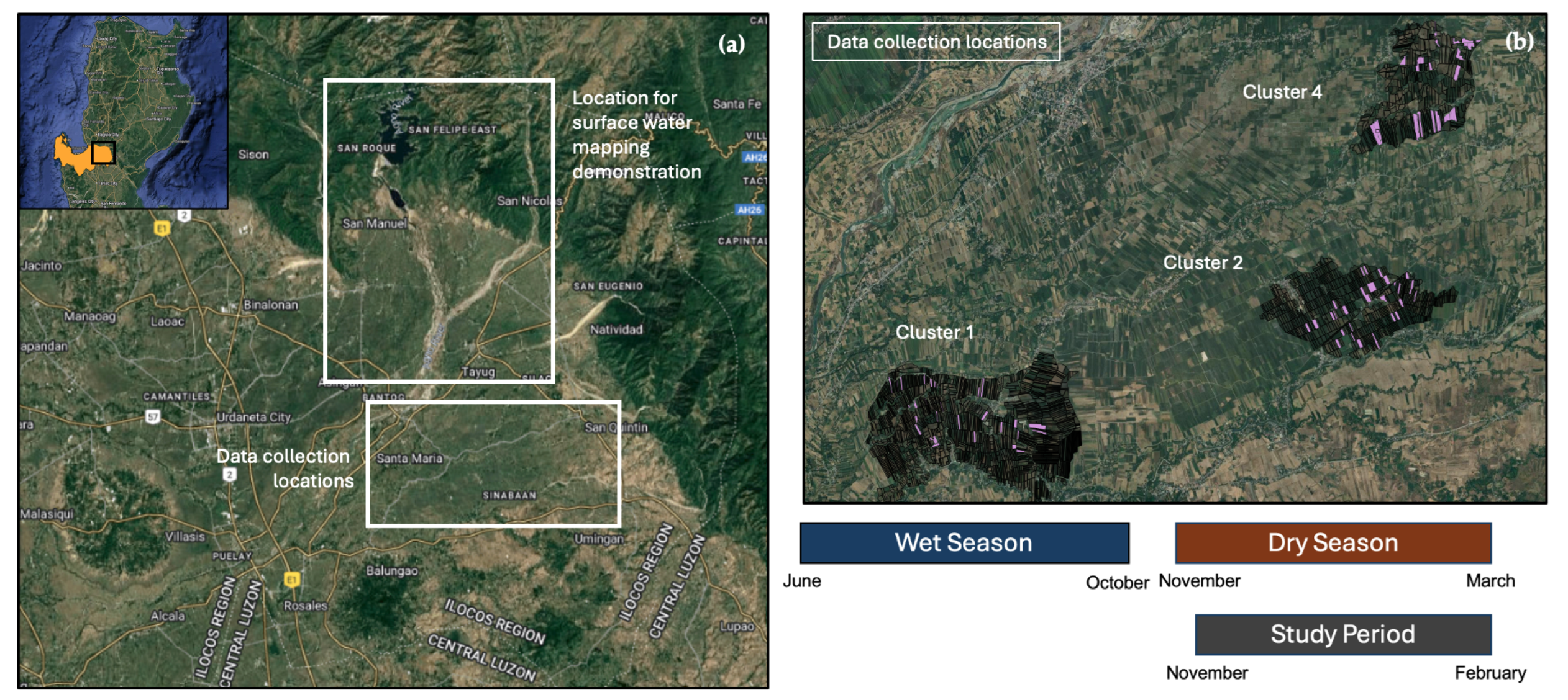
Figure 2.
Sample water level time series for selected fields, demonstrating the detection and removal of outliers after applying time-series smoothing. The plots highlight the unique water level variability for each field. (a)–(b) illustrate outliers caused by abrupt increases and decreases in water level, while (c) shows minimal to no detected outliers, indicating a stable time series throughout the season.
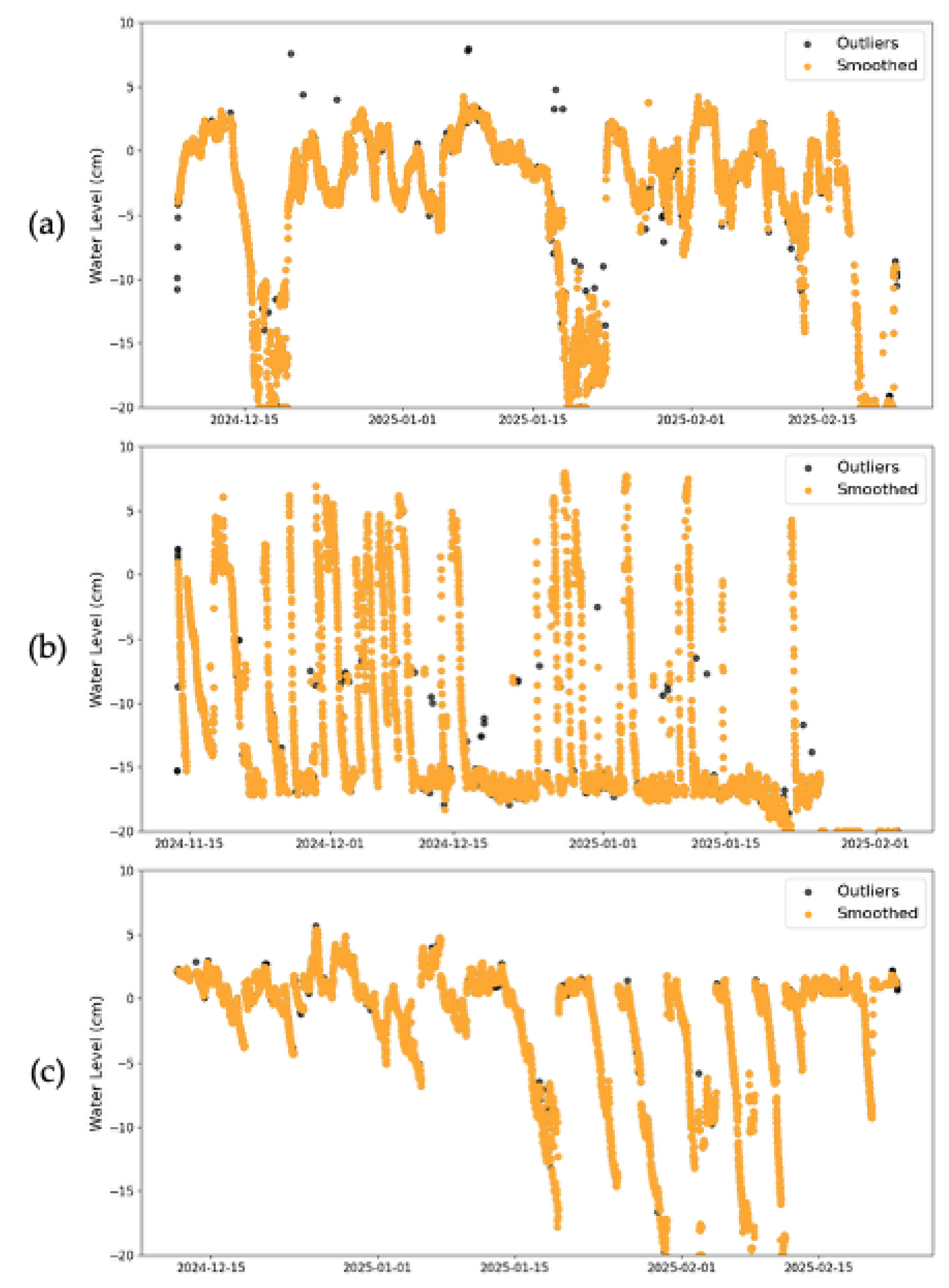
Figure 3.
(a) EVI boxplots throughout the 2024–2025 dry season cropping. (b) Data availability across the season, showing the number of water presence and absence occurrences for each satellite capture date. (c) Key rice growth stages: (1) transplanting, (2) tillering, (3) flowering, and (4) maturity before harvest, corresponding to observed EVI values, as confirmed by field personnel.
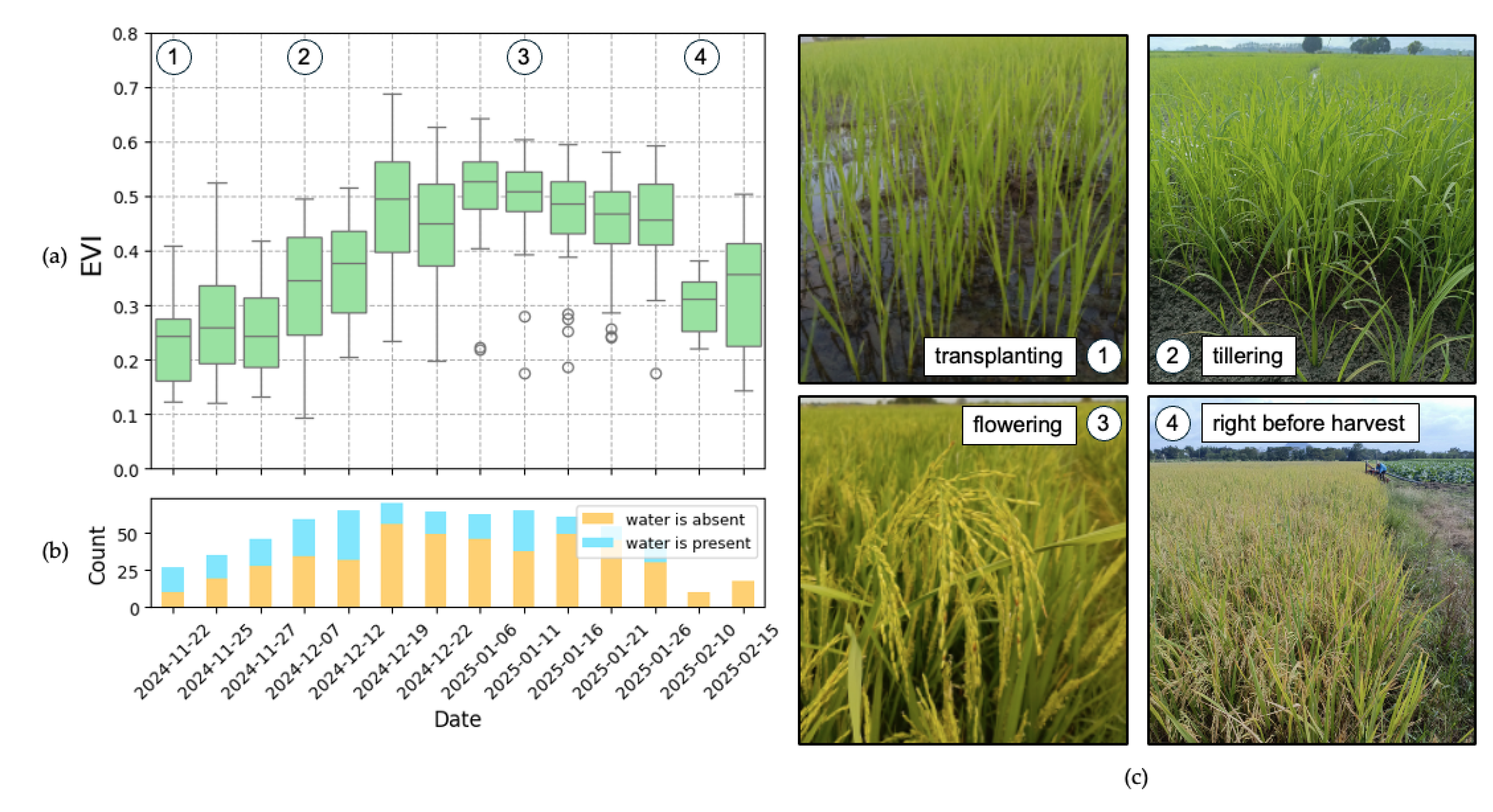
Figure 4.
Distribution of index values plotted against vegetation density, quantified by EVI. Blue dots represent data labeled as surface water presence, while orange dots indicate surface water absence. The solid black line represents the trendline illustrating the relationship between the index and vegetation density, while the red dashed line indicates the optimal threshold value for each index.
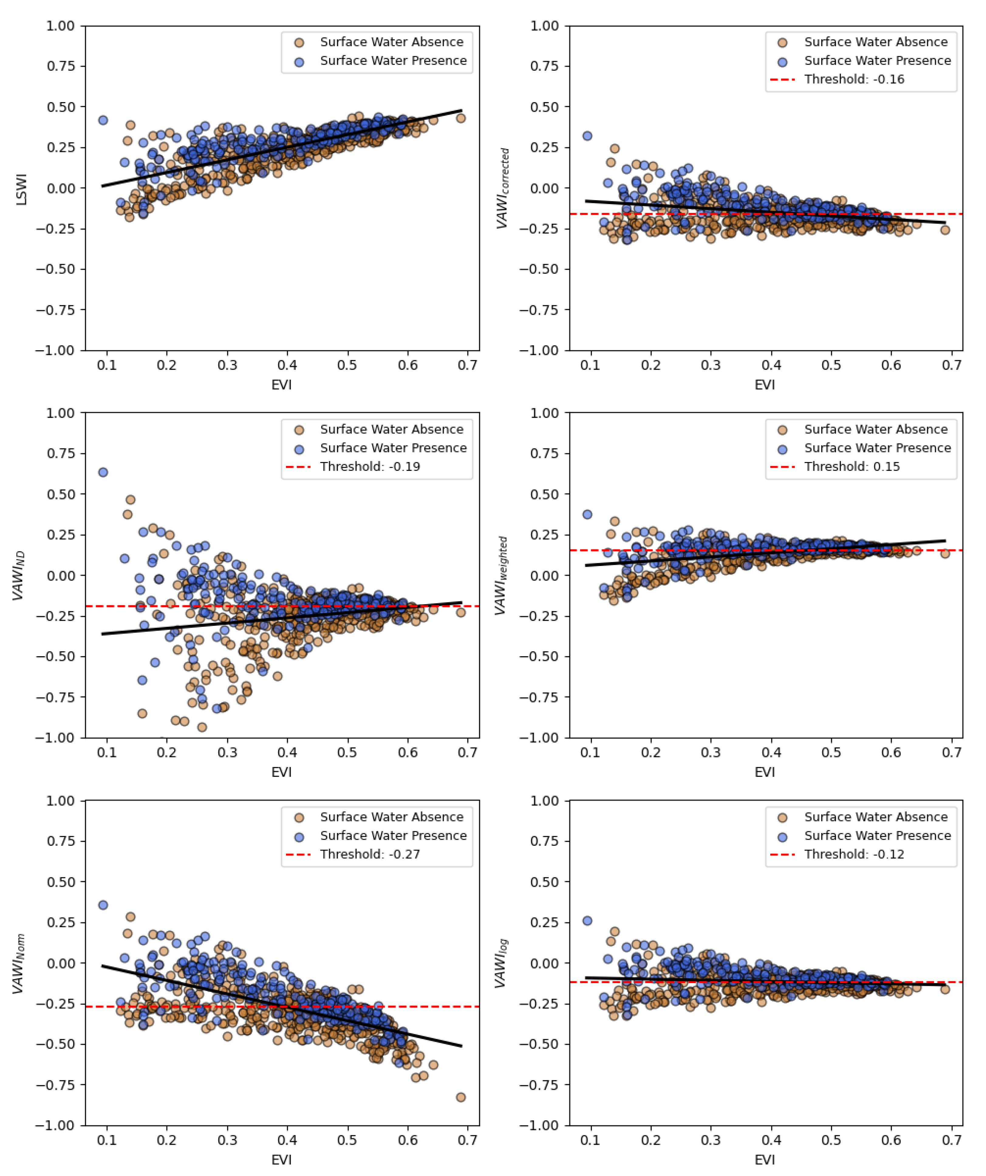
Figure 5.
Detection performance scores of the five LSWI–EVI transformations, presented as dot plots for balanced accuracy (BA), producer’s accuracy (PA), and user’s accuracy (UA).
Figure 5.
Detection performance scores of the five LSWI–EVI transformations, presented as dot plots for balanced accuracy (BA), producer’s accuracy (PA), and user’s accuracy (UA).
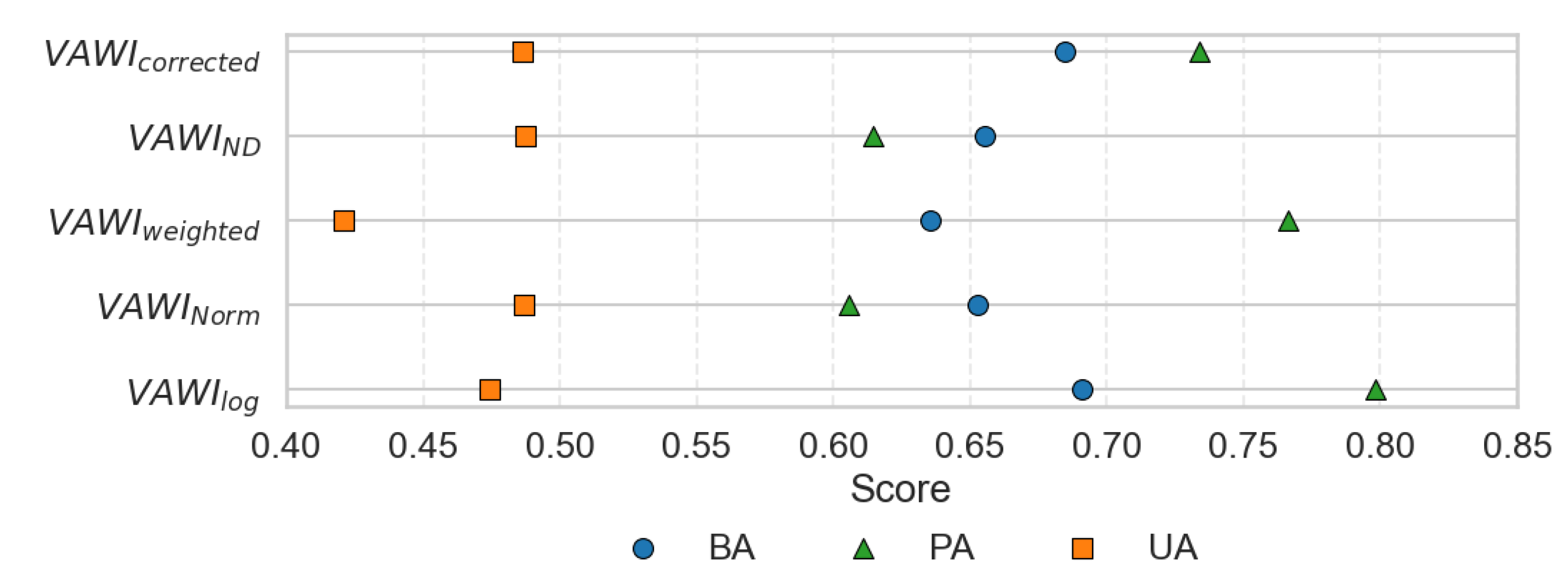
Figure 6.
Detection performance scores of VAWIlog against NDWI, LSWI, WIW and NDFI, presented as bar plots for balanced accuracy (BA), producer’s accuracy (PA), and user’s accuracy (UA).
Figure 6.
Detection performance scores of VAWIlog against NDWI, LSWI, WIW and NDFI, presented as bar plots for balanced accuracy (BA), producer’s accuracy (PA), and user’s accuracy (UA).
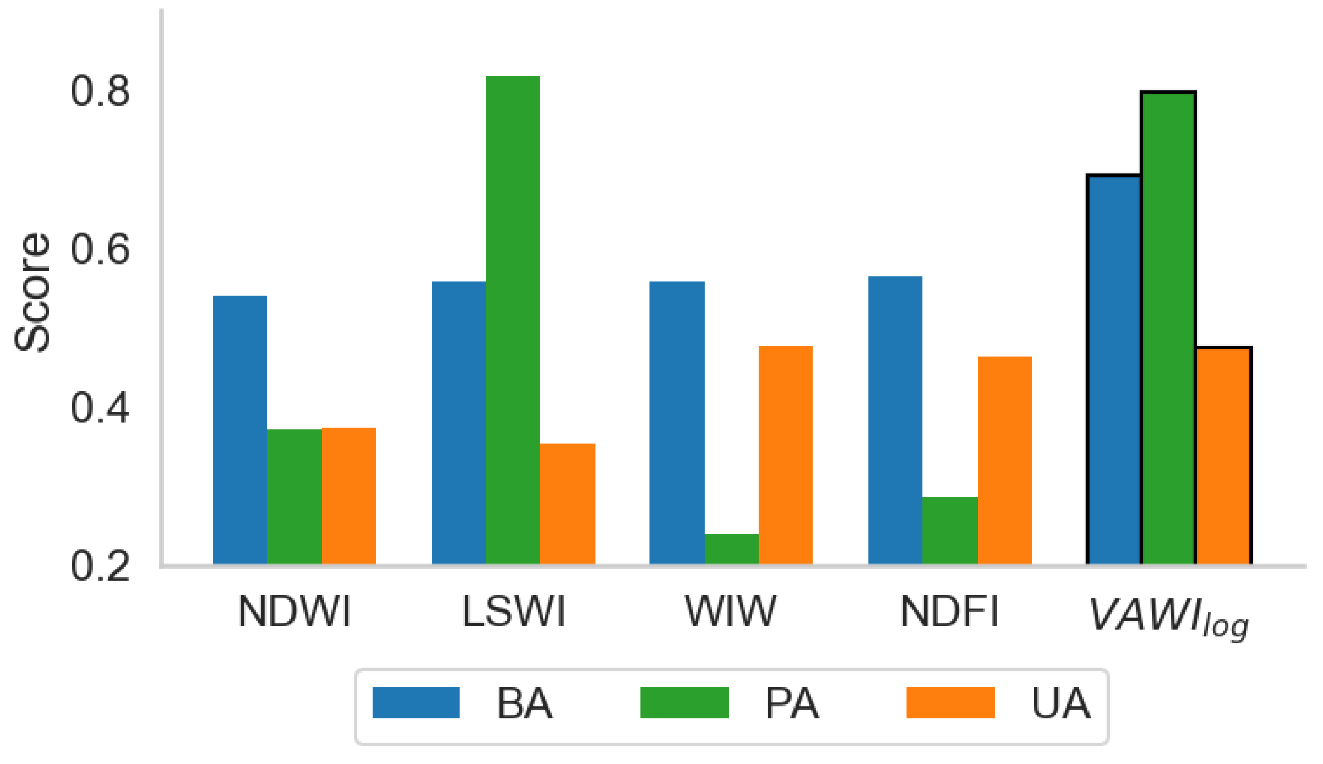
Figure 7.
Distribution of index values of NDWI, LSWI, NDFI and VAWIlog under surface water presence and absence conditions.
Figure 7.
Distribution of index values of NDWI, LSWI, NDFI and VAWIlog under surface water presence and absence conditions.
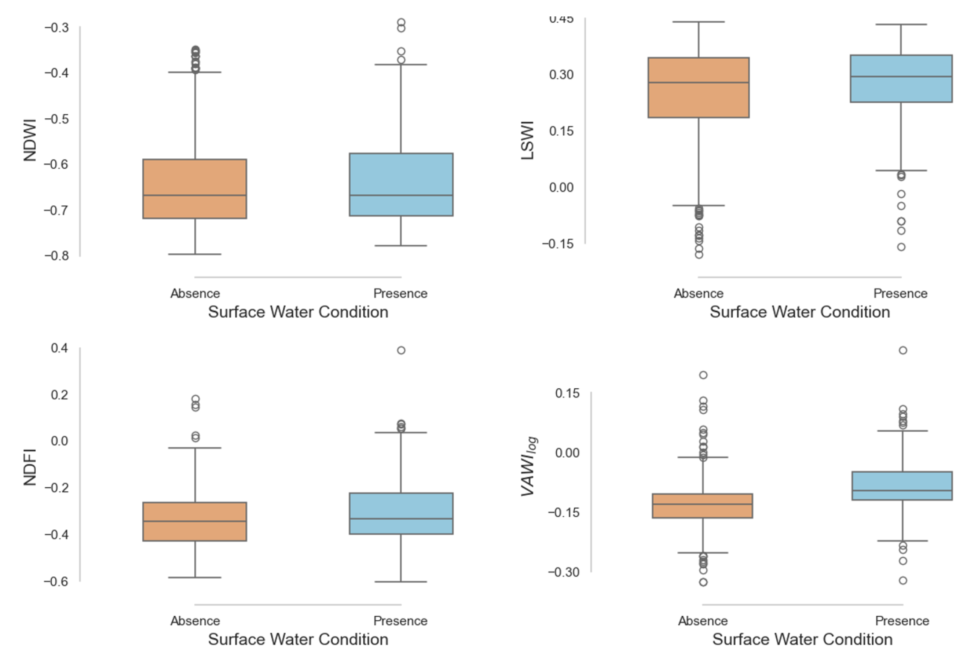
Figure 8.
(a) Balanced Accuracy and (b) Producer’s Accuracy of VAWIlog, NDWI, LSWI, WIW, and NDFI across increasing vegetation density, represented by EVI. (c) Frequency of surface water presence and absence instances per EVI interval, highlighting the consistent occurrence of surface water across all vegetation levels.
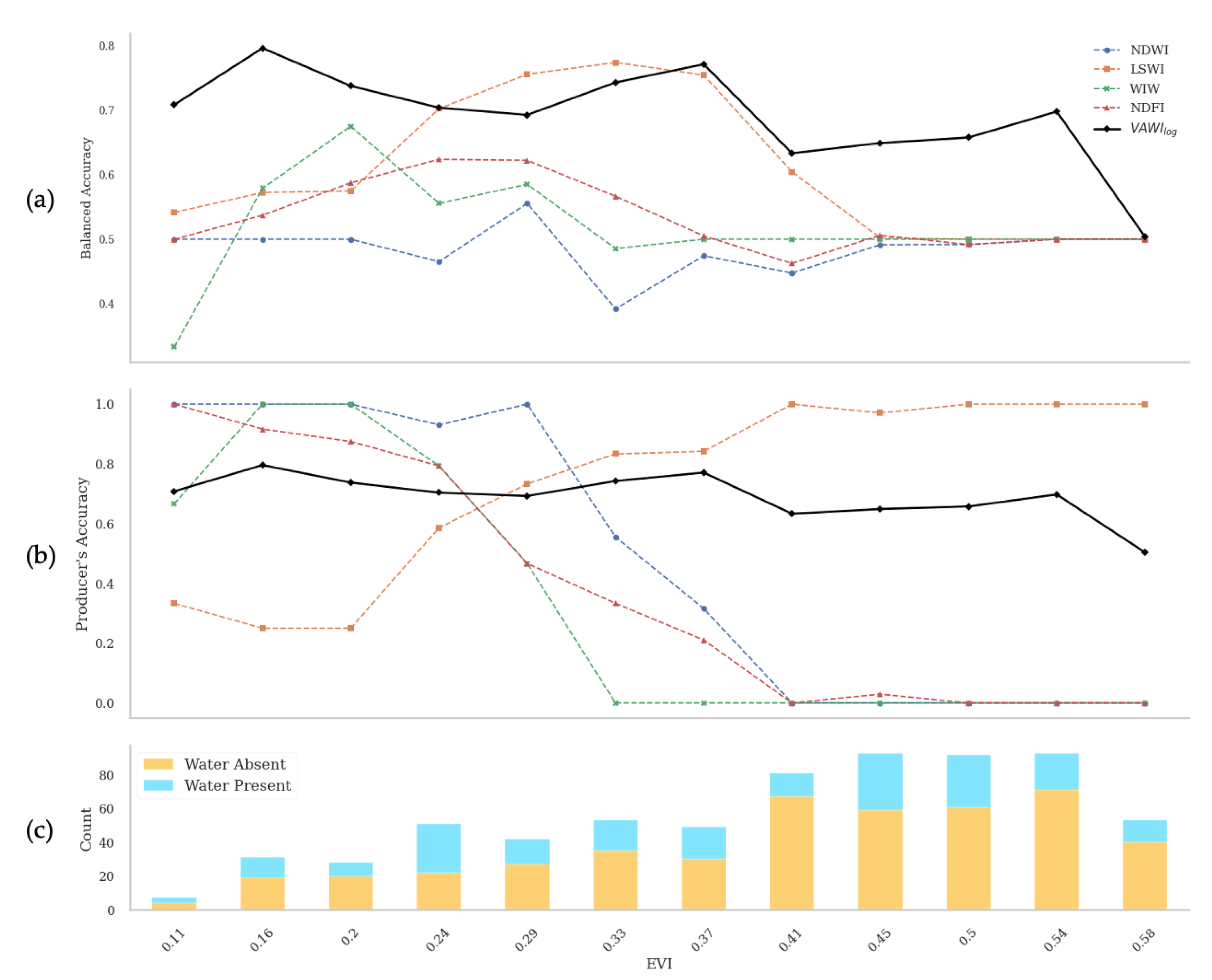
Figure 9.
Distribution of index values of NDWI, LSWI, NDFI and VAWIlog under surface water presence and absence conditions. Black dashed line is the computed optimum threshold for each index.
Figure 9.
Distribution of index values of NDWI, LSWI, NDFI and VAWIlog under surface water presence and absence conditions. Black dashed line is the computed optimum threshold for each index.
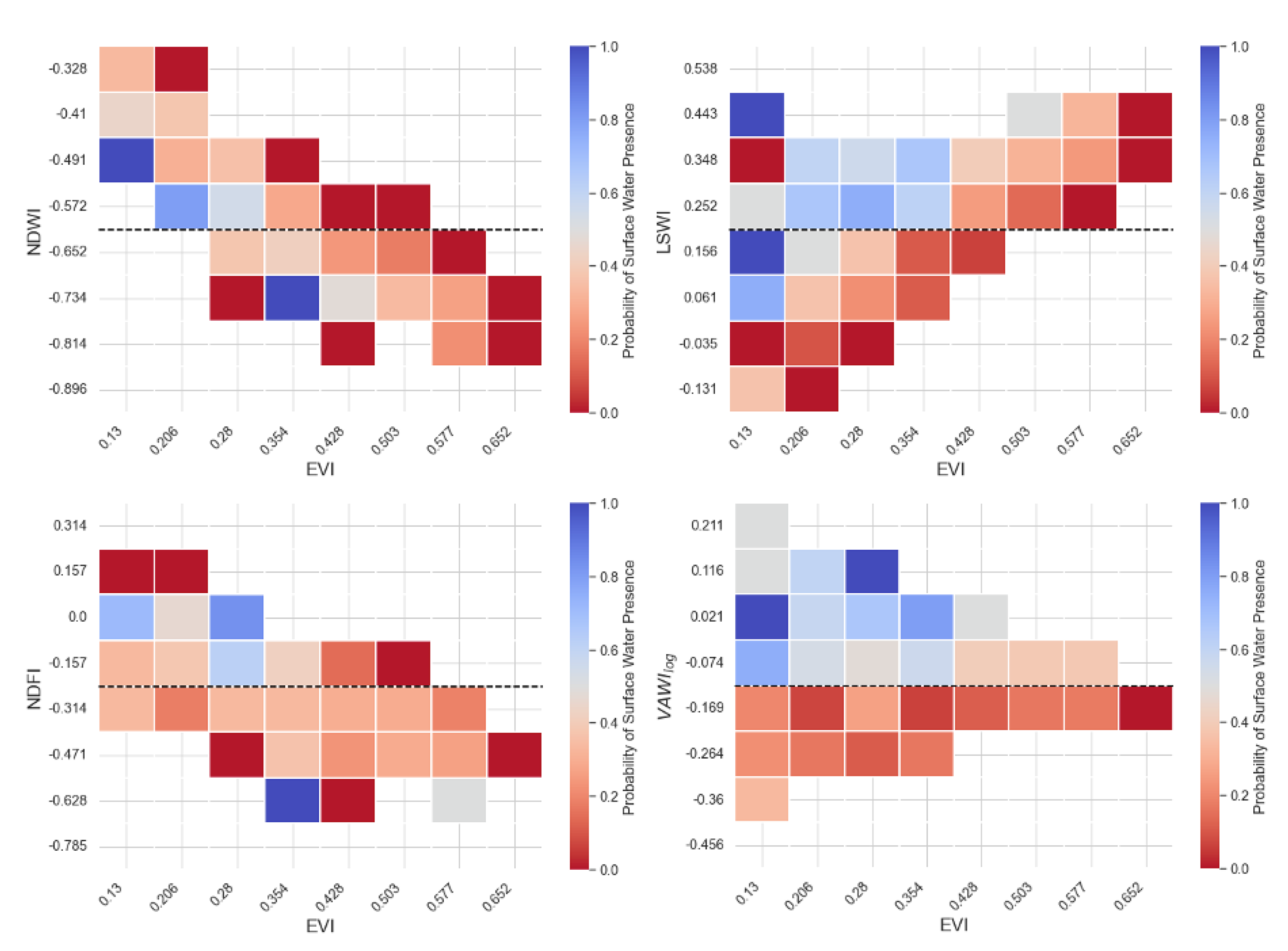
Figure 10.
(a) Proportion of Dynamic World land cover classifications across all rice-growing observation fields during the study period. (b) Simplified binary classification of surface water presence (water and flooded vegetation) versus absence (all other classes)for Dynamic World and VAWIlog
Figure 10.
(a) Proportion of Dynamic World land cover classifications across all rice-growing observation fields during the study period. (b) Simplified binary classification of surface water presence (water and flooded vegetation) versus absence (all other classes)for Dynamic World and VAWIlog
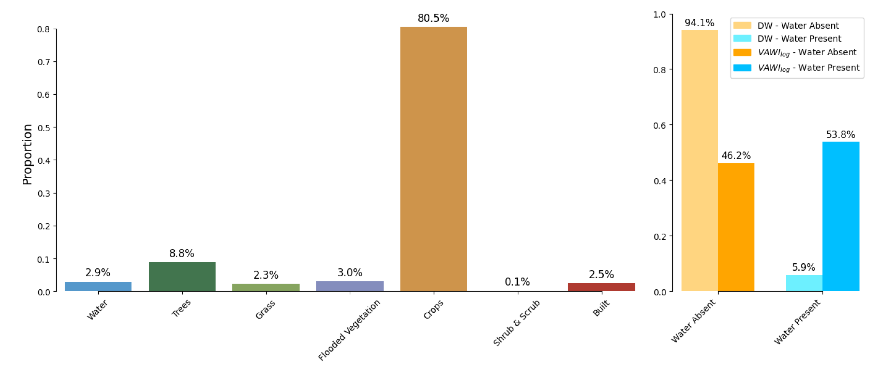
Figure 11.
Performance comparison between Dynamic World V1 and VAWIlog.
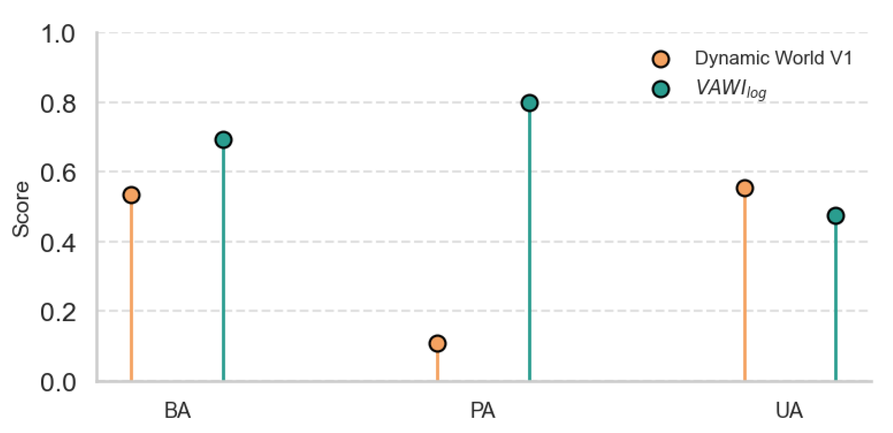
Figure 12.
EVI maps (first panels), NRT Dynamic World V1 land cover classifications (second panels), and surface water maps derived from VAWIlog (third panels) and NDWI (fourth panels) for Pangasinan, Philippines, on two observation dates: (a) 2025-01-21 and (b) 2025-02-25. The inclusion of EVI map panels provides additional context on vegetation density influencing water-vegetation separability. The appearance of slanted missing pixels is due to spatial grouping artifacts inherent in the Dynamic World classification algorithm.
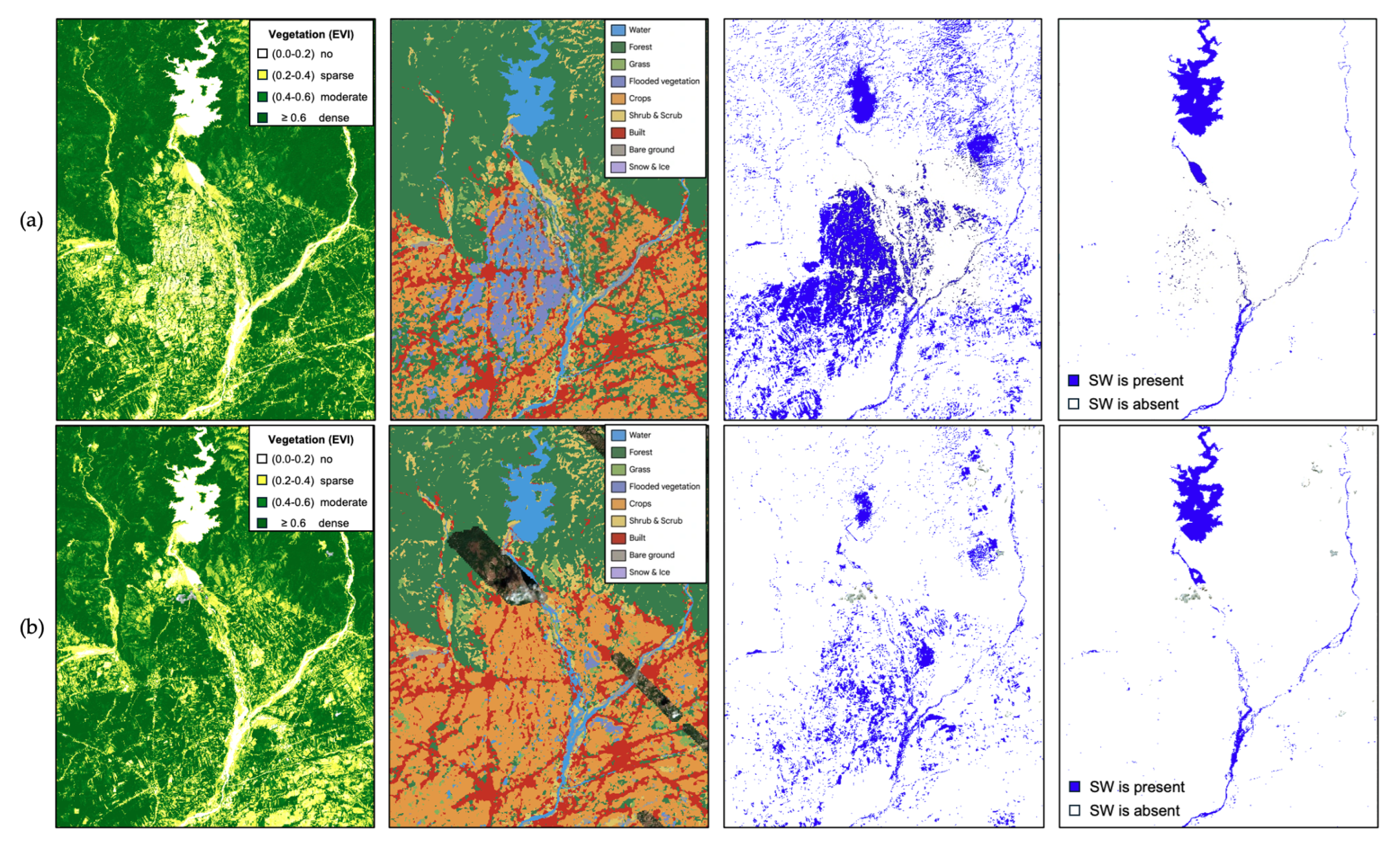
Figure 13.
Comprehensive surface water maps combining VAWIlog, NDWI and Dynamic World dataset for mapping surface water extent across different landscapes for (a) 2025-01-21 and (b) 2025-02-25. The appearance of slanted missing pixels is due to spatial grouping artifacts inherent in the Dynamic World classification algorithm.
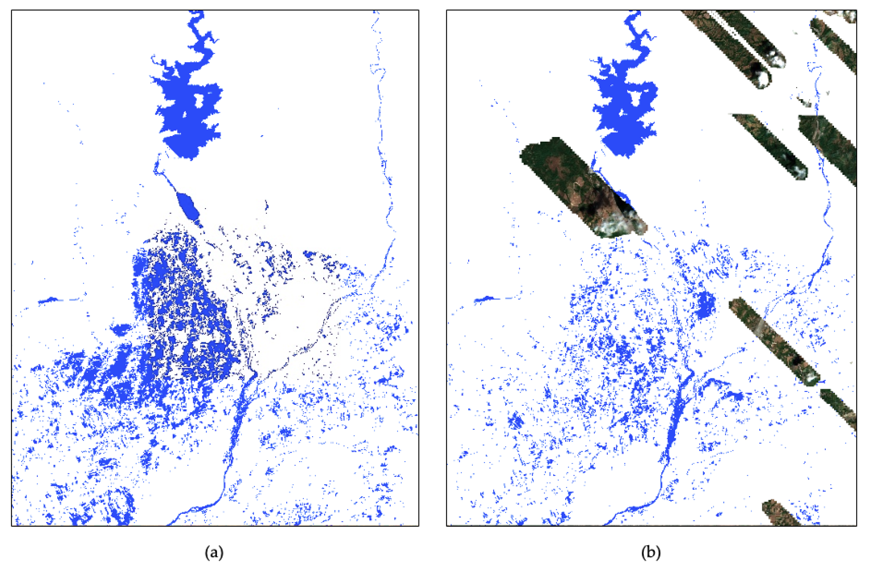

Table 1.
Mathematical formulations of vegetation-adjusted water index (VAWI) variants based on LSWI and EVI transformations.
Table 1.
Mathematical formulations of vegetation-adjusted water index (VAWI) variants based on LSWI and EVI transformations.
| LSWI - EVI Transformation | Formula |
|---|---|
| Simple Correction | |
| Normalized Difference | |
| Vegetation Weighted | |
| Vegetation Normalized | |
| Log Transformed |
1 is a small constant (e.g. ) added to maintain index stability.
Disclaimer/Publisher’s Note: The statements, opinions and data contained in all publications are solely those of the individual author(s) and contributor(s) and not of MDPI and/or the editor(s). MDPI and/or the editor(s) disclaim responsibility for any injury to people or property resulting from any ideas, methods, instructions or products referred to in the content. |
© 2025 by the authors. Licensee MDPI, Basel, Switzerland. This article is an open access article distributed under the terms and conditions of the Creative Commons Attribution (CC BY) license (http://creativecommons.org/licenses/by/4.0/).
Copyright: This open access article is published under a Creative Commons CC BY 4.0 license, which permit the free download, distribution, and reuse, provided that the author and preprint are cited in any reuse.


