
Submitted:
11 April 2024
Posted:
11 April 2024
You are already at the latest version
Abstract
(1) Background: A simple approach to map irrigated landcover has been introduced by using measures derived from optical spectral range as an alternative to thermal range. It has been demonstrated that substituting surface temperature (Ts, ‘thermal approach’) with SWIR transformed reflectance (STR, ‘optical approach’) to detect surface moisture is feasible with comparable results. (2) Methods: Using an iterative thresholding procedure to minimize within-class variance, the bilevel segmentation of variables derived from Landsat-8 representing surface moisture and vegetation cover was achieved for the 2020-21 summer for a key irrigation district in Australia. (3) Results: The results of irrigated landcover by optical approach found to be comparable with those by thermal approach. The classification accuracy was assessed using water delivery records at farm level. Though the overall accuracy is high in both cases, the optical approach (97.6%) performed slightly better than the thermal approach (93.9%). (4) Conclusions: The feasibility of using STR to map irrigated landcover has been confirmed by a high-level overall accuracy assessment. This has broader implications in terms of irrigated landcover assessment, as the use of satellite imagery in these applications may not necessarily be limited to microwave or thermal sensors.
Keywords:
Irrigated landcover
; thresholding method
; Central Goulburn District
1. Introduction
Irrigation is critical for agricultural production, and it plays an important role in food security in many areas of the world [1,2,3]. Irrigation not only increases crop yield by overcoming climatic constraints, but it also modifies local climatic conditions and adds to evapotranspiration [4,5]. In addition, irrigation can have some environmental impacts like increased soil salinity [6], changes in water table [7] and altered hydrological cycles [8]. The stated economic and ecological importance of irrigation warrants that the extent and distribution of irrigation is mapped precisely and monitored regularly.
Soil moisture is a key indicator of surface irrigation and irrigated landcover. The interaction of electromagnetic (EM) radiation with soil moisture and irrigated land has shown significant correlation at various wavelengths. As a result, several methods have been developed to map surface irrigation in different EM regions, namely optical, thermal and microwave. These methods have been summarised in detail in several recent studies [9,10,11,12]. As the microwave sensors are particularly sensitive to the changes in ground moisture, these have been used in mapping irrigated landcovers in many studies [13]. Though microwave sensors have provided promising results for the detection of irrigation in many areas, the coarse spatial resolution and the confounding effects of topography and vegetation created notable uncertainties in some regions [14]. However, the launch of Sentinel-1 satellites constellation (S1-A and S1-B) provided an unprecedented radar data coverage at a high spatial and temporal resolution. This has led to some new approaches of mapping irrigation, based on machine learning and empirical modelling, providing improved results [15,16].
Thermal infrared (TIR) sensors are considered highly relevant for irrigation mapping [17,18]. To distinguish between ‘irrigated’ and ‘non-irrigated’ land, TIR-derived surface temperature (Ts) has been widely used [19,20]. Ts is invariably used in combination with certain vegetation measures to map irrigated agriculture. There are very many vegetation indices which have been developed since the early attempts in 1960s - 1970s [21,22], frequently using a combination of spectral responses between visible and the near- or mid-infrared range [23]. The most used vegetation measure is the normalized difference vegetation index (NDVI), which is based on near-infrared (NIR) and red wavebands. Presently there are many satellites with optical sensors onboard, providing images suitable for vegetation indices at medium to high spatial resolution. However, there is a lack of satellites that provide thermal images with acceptable resolution, except for Landsat series of satellites (presently Landsat-8/9) which continues to provide concurrent thermal and optical observations at a nominal resolution of 30 m.
Though the thermal-based methods are powerful for irrigation mapping since they have physical rationale for their application, most methods depend on local weather conditions such as air temperature (Ta) close to the time of satellite overpass. The relationship between Ts and soil moisture is highly influenced by Ta and other atmospheric conditions [24]. Without the calibration of Ts, the results are likely to vary spatially across different landcovers, confounding the distinction of irrigated landcover. Considering this limitation, efforts have been made to find a robust substitute of Ts in the optical range to adequately account for surface moisture. Several indices that utilize optical observations have been proposed for the quantification of surface moisture or the lack of it, as shown in Table 1. Some of these indices are based on triangular or trapezoidal pixel distributions of optical observations in different spectral frequency range. It is notable that these optical indices (Table 1) are mostly empirical and lack any physical foundation. However, in a recent development, a method which is supported by both theory and experimental data, has been proposed by Sadeghi et al. [25]. This new method which has been designed to measure soil moisture is based on a linear model in shortwave infrared (SWIR) wavelengths, termed as ‘SWIR transformed reflectance’ (STR). We have chosen this measure to use in our study to explore its feasibility as a substitute of TIR-derived surface temperature for the mapping of irrigated land cover in the Central Goulburn Irrigation District (CGID) of Victoria, Australia, during the peak irrigation season (i.e., Summer) of 2020-21.
The objectives of this study are: (1) To assess the feasibility of using STR for mapping irrigated landcover; and (2) To compare TIR-based landcover classification (thermal approach) with STR-based landcover (optical approach).
3.1. Subsection
The CGID is located approximately between 36°04′41″S and 36°38′26″S latitudes, and between 144°46′37″E and 145°23′41″E longitudes, in the northern part of Victoria, Australia, (Figure 1). It is spread across the council jurisdiction of the Greater Shepparton City. It covers an area of about 1,900 sq. km., of which a large part is irrigated. The climate is temperate, and the region is relatively dry with average annual rainfall between 200 mm and 400 mm. In general, most of the rainfall is received during winter (June to August). Summers (December to February) are usually dry. The average maximum temperature ranges between 12° to 15°C in winter, increasing to 27° to 30°C in summer (December to February). The average minimum temperature varies from 3° to 6°C in winter to 12° to 15°C in summer (Figure 2). Victoria’s largest river, the Goulburn, flows on the eastern boundary before it joins the Australia’s largest river, the Murray, in the north. The flat terrain is covered by a network of irrigation channels. The irrigation systems used in the region include micro-irrigation, conventional sprinkler, flood, and furrow. The main industries are dairying, horticulture, cropping, and grazing.
2. Materials and Methods
The The study was undertaken in three broad steps. First, the satellite images were processed to generate the relevant measures for a representative date (8 Jan 2021) for the summer season. Second, a thresholding process was adopted to identify relative differences of surface temperature (Ts-Ta), surface moisture (STR) and vegetation status, which were then used to identify irrigated pixels. As a third step, the classified pixels were aggregated at farm scale as to match the irrigation water supply information and to measure the classification accuracy.
2.1. Satellite Data
A Landsat-8 Satellite Scene (Path 93/ Row 85) covered the study area. The image of this scene was taken from Landsat-8 Collection-2 Tier-1, which were calibrated as top-of-atmosphere (TOA) reflectance as follows [35]:
Elements of Equation (1) are:
= TOA reflectance [-]
= Constant equal to ~3.14159 [-]
Lλ = Spectral radiance [W/ (m2 sr μm)]
d = Earth-Sun distance [Astronomical units]
ESUNλ = Mean solar irradiance [W/ (m2 μm)]
θs = Solar zenith angle [Degrees]
Pixels with clouds, cloud shadows and cirrus clouds were masked out in the selected image.
2.2. Calculation of Surface Temperature (Ts)
At-sensor brightness temperature (Ts) was calculated using the following formula [35]:
Elements of Equation (2) are:
Ts = Effective at-sensor brightness temperature [K]
K2 = Calibration constant 2 [K]
K1 = Calibration constant 1 [W/(m2 sr μm)]
Lλ = Spectral radiance at the sensor’s aperture [W/(m2 sr μm)]
nl = Natural logarithm
For this study, Band 11 TIR2 (11500 - 12510 nm) was used for Lλ.
2.3. Surface-Air Temperature Difference (Ts−Ta)
Surface temperature has long been used to understand vegetation water status [36]. As plants transpire, water loss reduces leaf temperature due to evaporative cooling. The surface temperature of vegetation often becomes much lower than that of the surrounding air in situations of optimum water supply. Conversely, in water-stressed situations, vegetation transpires less and vegetation surface temperature increases, usually rising above the surrounding air temperature [37]. The difference between the surface and air temperatures (Ts−Ta) is therefore considered a logical variable to assess vegetation water status.
The air temperature data, close to the time of the satellite overpass, was sourced from the Bureau of Meteorology (www.bom.gov.au) and the SILO website (www.longpaddock.qld.gov.au/silo/) for multiple weather stations across and surrounding the study area. The point data of air temperature (Ta) was rasterized, using inverse distance weighted (IDW) method, to match the Ts from satellite.
2.4. Calculation of Shortwave-Infrared Transformed Reflectance (STR)
The concept of STR has been proposed by Sadeghi et al. [25] in relation to soil moisture. The derivation of STR is based on a simple model of Kubelka-Munk theory [38], which describes radiative transfer with absorption (k) and scattering (s) in a soil layer, considering a downward and an upward light propagation flux, perpendicular to the layer. By analytical solution of the equations for absorption and scattering coefficients, reflectance (R) is obtainable as the function of k and s [39]:
Sadeghi et al. [25] tested Equation (4) for soil moisture using multiple spectral frequencies in laboratory conditions, and found that SWIR bands (wavelength between 350 and 2500 nm) are optimal for soil moisture detection. Therefore Equation (4) was qualified as ‘SWIR transformed reflectance’ (STR) [40]:
2.5. Calculation of Vegetation and Water Indices
NIR denotes Band 5 (865 nm) and Red Band 4 (655 nm). NDVI was one of two key variables in land cover classification.
Normalised difference water index (NDWI) was calculated as follows [27]:
Green denotes Band 3 (560 nm). NDWI was used to detect and mask out surface water to ensure the STR estimates were confined to soil moisture.
2.6. Thresholding Process for Landcover Classification
An operational classification approach based on iterative thresholds has been adopted for this study. This approach, that generates bilevel classes of satellite-derived measures, has been previously used for the landcover classification in the irrigation regions [46,47]. Here we describe the process of both approaches: Optical and thermal.
It is widely accepted that an ‘irrigated’ crop has high vegetation and high soil moisture as compared to non-irrigated crops or other dry landcovers. On this basis, STR (soil moisture indicator) and NDVI (vegetation status) were segmented into two classes each. STR classes referred to ‘irrigated’ (relatively high soil moisture) and ‘non-irrigated’ (relatively low soil moisture), and vegetation classes were ‘crop’ (relatively high NDVI) and ‘non-crop’ (relatively low NDVI). An iterative thresholding method was used to achieve the binary classification by minimizing within-class variance, [48]:
Here, is the threshold which varies by iteration i, ω0 and ω1 are the weights of the two classes; and and are the variance of the two classes.
For applying the thresholding procedure in operation, the relationship of with between-class variance () and total variance () was made use of as follows [48]:
Initial NDVI threshold (α) was taken as 0.4. All pixels ≥α were considered as ‘crop’. Initial soil moisture threshold was the median value of STR (φ) or Ts-Ta (β). The iteration interval was set at 0.005 within the limit of ±0.025 of the initial thresholds. Altogether, 11 iterations each for NDVI and STR/Ts-Ta were performed for the image. Thresholds with minimum σ2Within were used for binary classification.
In the context of the ‘optical approach’, each pixel was identified with the defined binary classes of NDVI and STR. This resulted in four combinations as shown in Figure 3A. Pixels in sector (1) denote dry conditions with no or low vegetation. Pixels in sector (2) denote wet conditions with low or no vegetation. Pixels in sector (3) indicate some vegetation, which may be crop or pasture but without irrigation. Sector (4) denotes vegetation with wet condition indicating irrigated crop or pasture.
In the context of the ‘thermal approach’, the thresholding process for both NDVI and Ts-Ta was the same as described earlier. As shown in Figure 3B, the four sectors define the vegetation status and wet/dry conditions. Here as well the pixels in Sector (4) indicate irrigated crop or pasture.
Validation was carried out on the pixels aggregated to the extent of irrigation water delivery licences. Water delivery for each license has been linked to spatial unit consisting of one or more paddocks. These units hereinafter are referred to as farms. The mapped results of irrigated landcover were compared with the actual irrigation deliveries to farms. Information on irrigation water supplies at farm level was sourced from the Victorian Water Register (VWR), a state-wide irrigation water database (https://waterregister.vic.gov.au/). Figure 4 shows the location of farms which have been included in the validation process. In this figure, the locations of farms have been shown by farm centroids instead of farm boundaries due to privacy reason.
3. Results
3.1. Distribution of Input Measures
The classification process takes two variables as inputs in both approaches – ‘optical’ and ‘thermal’. NDVI is one variable, which is a common measure used in both approaches, as shown in Figure 5A. Though the NDVI ranges between 0 and ≥ 0.8 in CGID, the notable areas are those with NDVI ≥ 0.4 shown as shades of green. These areas are predominantly under perennial horticulture, perennial pastures, or summer crops. The NDVI distribution appears patchy and irregular mainly due to the widely varying sizes of agricultural properties ranging between under 2 ha and over 1000 ha.
The values of STR in CGID range between 0 and ≥ 10 (Figure 5B). However, the notable areas are those with STR values of 2 and over, indicating the presence of substantial surface moisture. Here the distinction must be made between potential irrigation areas, which are exclusively agricultural properties, and the riverine zone of native vegetation where the source of surface moisture is not irrigation.
Figure 5C shows the distribution of NDWI in CGID. All NDWI values above zero indicate presence of surface water. In addition to a few large water bodies like Waranga Basin in the south-central part, farm dams of varying sizes are shown across the district. The areas with surface water have been excluded while evaluating STR values.
The ‘Ts-Ta’ as an input variable for thermal approach of classification is largely driven by the satellite-derived surface temperature (Ts), moderated by air temperature (Ta). The spatial variation of Ta in CGID was within 3°- 4°C (Figure 5D). It ranged between under 21°C and about 24°C, increasing from south-east to north-west direction (Figure 5D). On the other hand, Ts ranged between 26° and over 40°C. Relatively cooler surfaces were with < 34°C, roughly spread in patches but largely contiguous in the riverine areas in the east (Figure 5E).
The distribution of Ts-Ta in CGID ranged between 0° and 24°C (Figure 5F). Here, the relatively cooler areas appear more pronounced as compared to those in Ts.
3.2. Thresholds for Pixel Classification
The Figure 6A,B show the identification of pixels as per optical and thermal approaches. Using Equation (9), the iteration process provided threshold for NDVI as 0.425, for STR as 1.425 and for Ts-Ta as 14.85°C. In each case, pixels have been divided into four classes. Pixels within Sector Four (refer to Figures 3A and 3B) have been identified as ‘irrigated’ crop or pasture.
3.3. Irrigated Landcover Classification
The Figure 7 shows the results of the irrigated landcover classification for optical approach. Figure 7A shows the four classes as identified in Figure 6A. Figure 7B is the map of irrigated landcover class only. Figure 8 shows the results of the irrigated landcover classification based on thermal approach where Figure 8A shows the four classes as identified in Figure 6B. Figure 8B is the map of irrigated landcover class only.
3.4. Validation of Irrigated Landcover
As stated earlier, validation of irrigated land cover classification has been carried out at farm level. Farms ≥10 ha in size were selected for validation. A farm was considered as ‘irrigated’ (‘Reference’) based on a substantive amount of water delivery (≥0.1 ML per ha) to that farm during the timeframe of the summer season (December to February). No or negligible amount of water delivery (<0.1 ML per ha) was taken as the absence of irrigation on a farm. These reference farms were compared with the classification results for accuracy.
As per the classification, a farm was considered ‘irrigated’ provided a substantial proportion of pixels (≥25%) within that farm belonged to Sector 4 (Wet and active vegetation; Refer Figure 3 and Figure 6). This criterion was uniformly applied to both optical and thermal approaches.
Table 2 and Table 3 provide classification accuracy for the two approaches. The calculation of confusion matrix resulting into producer’s and user’s accuracies followed standard procedure [49,50]. Though the overall accuracy is high in both cases, the optical approach (97.6%) performed slightly better than the thermal approach (93.9%). The user’s accuracy for irrigated landcover was noticeably higher in case of optical approach (98.3%) as compared to that of thermal approach (88%). However, there is very little difference between the two approaches as per producer’s accuracy for irrigated landcover (96.2% for optical and 97.1 for thermal).
4. Discussion
The feasibility of using STR along with NDVI (optical approach) to map irrigated landcover has been confirmed by a high-level overall accuracy assessment (97.6%). These results of irrigated landcover by optical approach found to be comparable with those of a parallel process that used Ts-Ta along with NDVI (thermal approach). However, there was a noticeable difference in the user’s accuracy for the ‘irrigated’ class between the two approaches (88% thermal to 98.3% optical). This could have occurred due to the difference in the spatial resolution of a variable for surface moisture. STR is based on Band 7 of Landsat 8 which has 30m resolution, whereas Band 11 used in Ts-Ta is 100m resolution though resampled to 30m [51].
The threshold-based classification used in this study is an example of a simple and operational approach for routine monitoring of irrigated landcover. The initial threshold for NDVI (0.4) was on the assumption that, in an agriculture enterprise, vegetation with NDVI < 0.4 is unlikely to be a managed crop or pasture. In the case of STR and Ts-Ta, the initial threshold taken was the median pixel value of the variable, which was based on the experience from the previous studies in the region [46,47,52]. These initial thresholds and the related assumptions should be field tested further to ascertain the strengths and weaknesses of this approach in different landscapes and at different times.
The classification method used in this study assumes that the main source of surface moisture is irrigation and rainfall does not have any significant impact. As stated earlier, the summers in the study area are generally dry. The long-term average of rainfall during the three months of summer is 101.8mm (Figure 2). The study period (December 2020 to February 2021) was, however, drier with a total of 80.6mm. In case of high rainfall situations, there will be a requirement of season-wide vegetation as well as STR analysis of the known irrigated and dryland farms vis-à-vis rainfall records to make the desired adjustments to thresholding method.
This study used a single image as a representative of summer season. This is in accordance with a previous study in the irrigation regions of Victoria, Australia, which found the use of single ‘midseason’ image adequate to assess maximum crop cover because of strong temporal stability in NDVI response [53]. However, for further studies, there is a scope to test temporal aggregates of image-based variables from multiple sources including Landsat-8/9 and Sentinel-2.
This study is a formal affirmation of using STR as a substitute of Ts-based measures for irrigated landcover classification. The basis of this affirmation is the formal comparison of optical approach with thermal approach implemented in a key irrigation district. This opens the opportunity of utilising the widely available optical sensors for irrigated landcover investigations.
5. Conclusions
The satellite-derived surface moisture (STR, Ts) and vegetation status (NDVI) are appropriate measures to distinguish between irrigated and non-irrigated pixels within farmlands. The use of STR, which is based on Band 7 of Landsat-8 (optical spectral range), with NDVI demonstrated successful mapping of irrigated landcover for the summer season of 2020-21 in CGID. The results of this optical approach of classification are found to be comparable with those of thermal approach where Ts-Ta is used with NDVI for classification. These results have broader implications in terms of irrigated landcover assessment, as the use of satellite imagery in these applications may not necessarily be limited to sensors with either microwave or thermal bands. The impact of this is a greater freedom, both spatially and temporally, to develop this information.
Author Contributions
Conceptualization, M.A. and A.M.; methodology, M.A.; validation, A.M., M.A. and K.S.; formal analysis, M.A.; resources, A.M.; writing—original draft preparation, M.A.; writing—review and editing, K.S. and M.A.; project administration, A.M. and M.A. All authors have read and agreed to the published version of the manuscript.
Funding
This research received no external funding.
Data Availability Statement
Data sets are not available due to privacy reason of individual farm holders.
Acknowledgments
Authors are thankful to the leadership team of Agriculture Victoria Research for the support of the work.
Conflicts of Interest
The authors declare no conflicts of interest.
References
- Massari, C.; Modanesi, S.; Dari, J.; Gruber, A.; De Lannoy, G.J.M.; Girotto, M.; Quintana-Seguí, P.; Le Page, M.; Jarlan, L.; Zribi, M.; et al. A review of irrigation information retrievals from space and their utility for users. Remote Sensing 2021, 13, 4112. [CrossRef]
- Weiss, M.; Jacob, F.; Duveiller, G. Remote sensing for agricultural applications: A meta-review. Remote Sensing of Environment 2020, 236, 111402. [CrossRef]
- World Bank. Water in agriculture. In https://www.worldbank.org/en/topic/water-in-agriculture, [Last accessed on 1 Sep 2023], 2022.
- Ketchum, D.; Jencso, K.; Maneta, M.P.; Melton, F.; Jones, M.O.; Huntington, J. Irrmapper: A machine learning approach for high resolution mapping of irrigated agriculture across the western U.S. Remote Sensing 2020, 12. [CrossRef]
- Liu, J.; Jin, J.; Niu, G.-Y. Effects of irrigation on seasonal and annual temperature and precipitation over china simulated by the wrf model. Journal of Geophysical Research: Atmospheres 2021, 126, e2020JD034222. [CrossRef]
- Mohanavelu, A.; Naganna, S.R.; Al-Ansari, N. Irrigation induced salinity and sodicity hazards on soil and groundwater: An overview of its causes, impacts and mitigation strategies. Agriculture 2021, 11, 983. [CrossRef]
- Haacker, E.M.; Kendall, A.D.; Hyndman, D.W. Water level declines in the high plains aquifer: Predevelopment to resource senescence. Ground water 2016, 54, 231-242. [CrossRef]
- Coleman, R.W.; Stavros, N.; Hulley, G.; Parazoo, N. Comparison of thermal infrared-derived maps of irrigated and non-irrigated vegetation in urban and non-urban areas of southern california. Remote Sensing 2020, 12, 1-19. [CrossRef]
- Zhang, D.; Zhou, G. Estimation of soil moisture from optical and thermal remote sensing: A review. Sensors (Basel, Switzerland) 2016, 16. [CrossRef]
- Babaeian, E.; Sadeghi, M.; Jones, S.B.; Montzka, C.; Vereecken, H.; Tuller, M. Ground, proximal, and satellite remote sensing of soil moisture. Reviews of Geophysics 2019, 57, 530-616. [CrossRef]
- Sultana, M.S.; Gazi, M.Y.; Mia, M.B. Multiple indices based agricultural drought assessment in the northwestern part of bangladesh using geospatial techniques. Environmental Challenges 2021, 4, 100120. [CrossRef]
- Li, Z.-L.; Leng, P.; Zhou, C.; Chen, K.-S.; Zhou, F.-C.; Shang, G.-F. Soil moisture retrieval from remote sensing measurements: Current knowledge and directions for the future. Earth-Science Reviews 2021, 218, 103673. [CrossRef]
- Bazzi, H.; Baghdadi, N.; Fayad, I.; Zribi, M.; Belhouchette, H.; Demarez, V. Near real-time irrigation detection at plot scale using sentinel-1 data. Remote Sensing 2020, 12, 1456. [CrossRef]
- Kumar, S.V.; Peters-Lidard, C.D.; Santanello, J.A.; Reichle, R.H.; Draper, C.S.; Koster, R.D.; Nearing, G.; Jasinski, M.F. Evaluating the utility of satellite soil moisture retrievals over irrigated areas and the ability of land data assimilation methods to correct for unmodeled processes. Hydrol. Earth Syst. Sci. 2015, 19, 4463-4478. [CrossRef]
- El Hajj, M.; Baghdadi, N.; Zribi, M.; Bazzi, H. Synergic use of sentinel-1 and sentinel-2 images for operational soil moisture mapping at high spatial resolution over agricultural areas. Remote Sensing 2017, 9, 1292. [CrossRef]
- Bousbih, S.; Zribi, M.; El Hajj, M.; Baghdadi, N.; Lili-Chabaane, Z.; Gao, Q.; Fanise, P. Soil moisture and irrigation mapping in a semi-arid region, based on the synergetic use of sentinel-1 and sentinel-2 data. Remote Sensing 2018, 10, 1953. [CrossRef]
- Cheng, J.; Kustas, W.P. Using very high resolution thermal infrared imagery for more accurate determination of the impact of land cover differences on evapotranspiration in an irrigated agricultural area. Remote Sensing 2019, 11. [CrossRef]
- Chatterjee, S.; Desai, A.R.; Zhu, J.; Townsend, P.A.; Huang, J. Soil moisture as an essential component for delineating and forecasting agricultural rather than meteorological drought. Remote Sensing of Environment 2022, 269. [CrossRef]
- Ozdogan, M., Gutman, G. A new methodology to map irrigated areas using multi-temporal modis and ancillary data: An application example in the continental us. Remote Sensing of Environment 2008, 112, 3520-3537. [CrossRef]
- Ozdogan, M.; Yang, Y.; Allez, G.; Cervantes, C. Remote sensing of irrigated agriculture: Opportunities and challenges. Remote Sensing 2010, 2, 2274-2304. [CrossRef]
- Jordan, C.F. Derivation of leaf-area index from quality of light on the forest floor. Ecology 1969, 50, 663-666. [CrossRef]
- Rouse, J.W.; Haas, R.H.; Schell, J.A.; Deering, D.W. Monitoring vegetation systems in the great plains with erts. In Third ERTS Symposium, NASA: Washington, DC, 1973; Vol. 1, pp 309-317.
- Hatfield, J.L.; Prueger, J.H.; Sauer, T.J.; Dold, C.; O’Brien, P.; Wacha, K. Applications of vegetative indices from remote sensing to agriculture: Past and future. Inventions 2019, 4, 71. [CrossRef]
- Czajkowski, K.; Goward, S.; Stadler, S.; Walz, A. Thermal remote sensing of near surface environmental variables: Application over the oklahoma mesonet. Professional Geographer - PROF GEOGR 2000, 52, 345-357. [CrossRef]
- Sadeghi, M.; Jones, S.B.; Philpot, W.D. A linear physically-based model for remote sensing of soil moisture using short wave infrared bands. Remote Sensing of Environment 2015, 164, 66-76. [CrossRef]
- Kogan, F.N. Application of vegetation index and brightness temperature for drought detection. Advances in Space Research 1995, 15, 91-100. [CrossRef]
- McFeeters, S.K. The use of the normalized difference water index (ndwi) in the delineation of open water features. International Journal of Remote Sensing 1996, 17, 1425-1432. [CrossRef]
- Wang, L.; Qu, J.J. Nmdi: A normalized multi-band drought index for monitoring soil and vegetation moisture with satellite remote sensing. Geophysical Research Letters 2007, 34, n/a-n/a. [CrossRef]
- Ghulam, A.; Qin, Q.; Zhan, Z. Designing of the perpendicular drought index. Environmental Geology 2007, 52, 1045-1052. [CrossRef]
- Ghulam, A.; Qin, Q.; Teyip, T.; Li, Z.-L. Modified perpendicular drought index (mpdi): A real-time drought monitoring method. ISPRS Journal of Photogrammetry and Remote Sensing 2007, 62, 150-164. [CrossRef]
- Feng, H.; Chen, C.; Dong, H.; Wang, J.; Meng, Q. Modified shortwave infrared perpendicular water stress index: A farmland water stress monitoring method. Journal of Applied Meteorology and Climatology 2013, 52, 2024-2032. [CrossRef]
- Yang, N.; Qin, Q.; Jin, C.; Yao, Y. In The comparison and application of the methods for monitoring farmland drought based on nir-red spectral space, IGARSS 2008 - 2008 IEEE International Geoscience and Remote Sensing Symposium, 7-11 July 2008, 2008; pp III - 871-III - 874.
- Zhang, N.; Hong, Y.; Qin, Q.; Liu, L. Vsdi: A visible and shortwave infrared drought index for monitoring soil and vegetation moisture based on optical remote sensing. International Journal of Remote Sensing 2013, 34, 4585-4609. [CrossRef]
- Fensholt, R.; Sandholt, I. Derivation of a shortwave infrared water stress index from modis near- and shortwave infrared data in a semiarid environment. Remote Sensing of Environment 2003, 87, 111-121. [CrossRef]
- Chander, G.; Markham, B.L.; Helder, D.L. Summary of current radiometric calibration coefficients for landsat mss, tm, etm+, and eo-1 ali sensors. Remote Sensing of Environment 2009, 113, 893-903. [CrossRef]
- Idso, S.B.; Jackson, R.D.; Pinter Jr, P.J.; Reginato, R.J.; Hatfield, J.L. Normalizing the stress-degree-day parameter for environmental variability. Agricultural Meteorology 1981, 24, 45-55. [CrossRef]
- Jackson, R.D. Canopy temperature and crop water stress. In Advances in irrigation, Hillel, D., Ed. Elsevier: 1982; Vol. 1, pp 43-85.
- Kubelka, P., Munk, Franz Ein beitrag zur optik der farbanstriche. Zeitschrift für Technische Physik 1931, 12, 593-601.
- Ciani, A.; Goss, K.U.; Schwarzenbach, R. Light penetration in soil and particulate minerals. European Journal of Soil Science 2005, 56, 561-574. [CrossRef]
- Sadeghi, M.; Babaeian, E.; Tuller, M.; Jones, S.B. The optical trapezoid model: A novel approach to remote sensing of soil moisture applied to sentinel-2 and landsat-8 observations. Remote Sensing of Environment 2017, 198, 52-68. [CrossRef]
- Hassanpour, R.; Zarehaghi, D.; Neyshabouri, M.R.; Feizizadeh, B.; Rahmati, M. Modification on optical trapezoid model for accurate estimation of soil moisture content in a maize growing field. Journal of Applied Remote Sensing 2020, 14, 034519. [CrossRef]
- Chen, M.; Zhang, Y.; Yao, Y.; Lu, J.; Pu, X.; Hu, T.; Wang, P. Evaluation of an optical trapezoid model (optram) to retrieve soil moisture in the sanjiang plain of northeast china. Earth and Space Science 2020, 7. [CrossRef]
- Wu, S.-W.; Huang, H.; Tsai, S.-F.; Lin, C.-Y. Identification of aeolian dust hotspots in the lower reaches of zhuoshui river in taiwan using environmental indicators. Ecological Indicators 2023, 154, 110864. [CrossRef]
- Mokhtari, A.; Sadeghi, M.; Afrasiabian, Y.; Yu, K. Optram-et: A novel approach to remote sensing of actual evapotranspiration applied to sentinel-2 and landsat-8 observations. Remote Sensing of Environment 2023, 286, 113443. [CrossRef]
- Abuzar, M., Sheffield, Kathryn, Whitfield, Des, O’Connell, Mark, McAllister, Andy. Comparing inter-sensor ndvi for the analysis of horticulture crops in south-eastern australia. American Journal of Remote Sensing 2014, 2, 1-9. [CrossRef]
- Abuzar, M.; McAllister, A.; Whitfield, D. Mapping irrigated farmlands using vegetation and thermal thresholds derived from landsat and aster data in an irrigation district of australia. Photogrammetric Engineering & Remote Sensing 2015, 81, 229-238. [CrossRef]
- Abuzar, M.M., A.; Whitfield, D.; Sheffield, K. Remotely-sensed surface temperature and vegetation status for the assessment of decadal change in the irrigated land cover of north-central victoria, australia. Land 2020, 9, 308. [CrossRef]
- Otsu, N. A threshold selection method from gray-level histograms. Systems, Man and Cybernetics, IEEE Transactions on 1979, 9, 62-66. [CrossRef]
- Congalton, R.G. A review of assessing the accuracy of classifications of remotely sensed data. Remote Sensing of Environment 1991, 37, 35-46. [CrossRef]
- Foody, G.M. Status of land cover classification accuracy assessment. Remote Sensing of Environment 2002, 80, 185-201. [CrossRef]
- USGS. Landsat 8 (l8) data users handbook. US Geological Survey: Sioux Falls, SD, 2019; p 106.
- Abuzar, M.; Whitfield, D.; McAllister, A. Farm level assessment of irrigation performance for dairy pastures in the goulburn-murray district of australia by combining satellite-based measures with weather and water delivery information. ISPRS International Journal of Geo-Information 2017, 6, 239. [CrossRef]
- O’Connell, M.G. Satellite based yield: Water use relationships of perennial horticultural crops (PhD thesis). University of Melbourne, Melbourne, 2011.
Figure 1.
The study area. (a) CGID location in Australia, and (b) Extent of CGID (in yellow) with the background of Landsat-8 satellite image bands 5/4/3(displayed as a false colour composite image).
Figure 1.
The study area. (a) CGID location in Australia, and (b) Extent of CGID (in yellow) with the background of Landsat-8 satellite image bands 5/4/3(displayed as a false colour composite image).
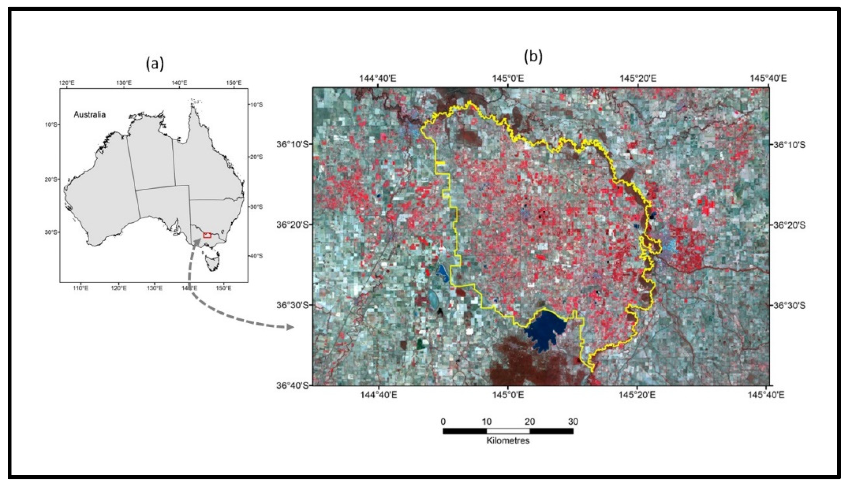
Figure 2.
Average monthly rainfall and minimum/maximum temperatures at the Tatura weather station (Latitude: 36.44 °S; Longitude: 145.27 °E; Elevation: 114 m), located within the study area.
Figure 2.
Average monthly rainfall and minimum/maximum temperatures at the Tatura weather station (Latitude: 36.44 °S; Longitude: 145.27 °E; Elevation: 114 m), located within the study area.
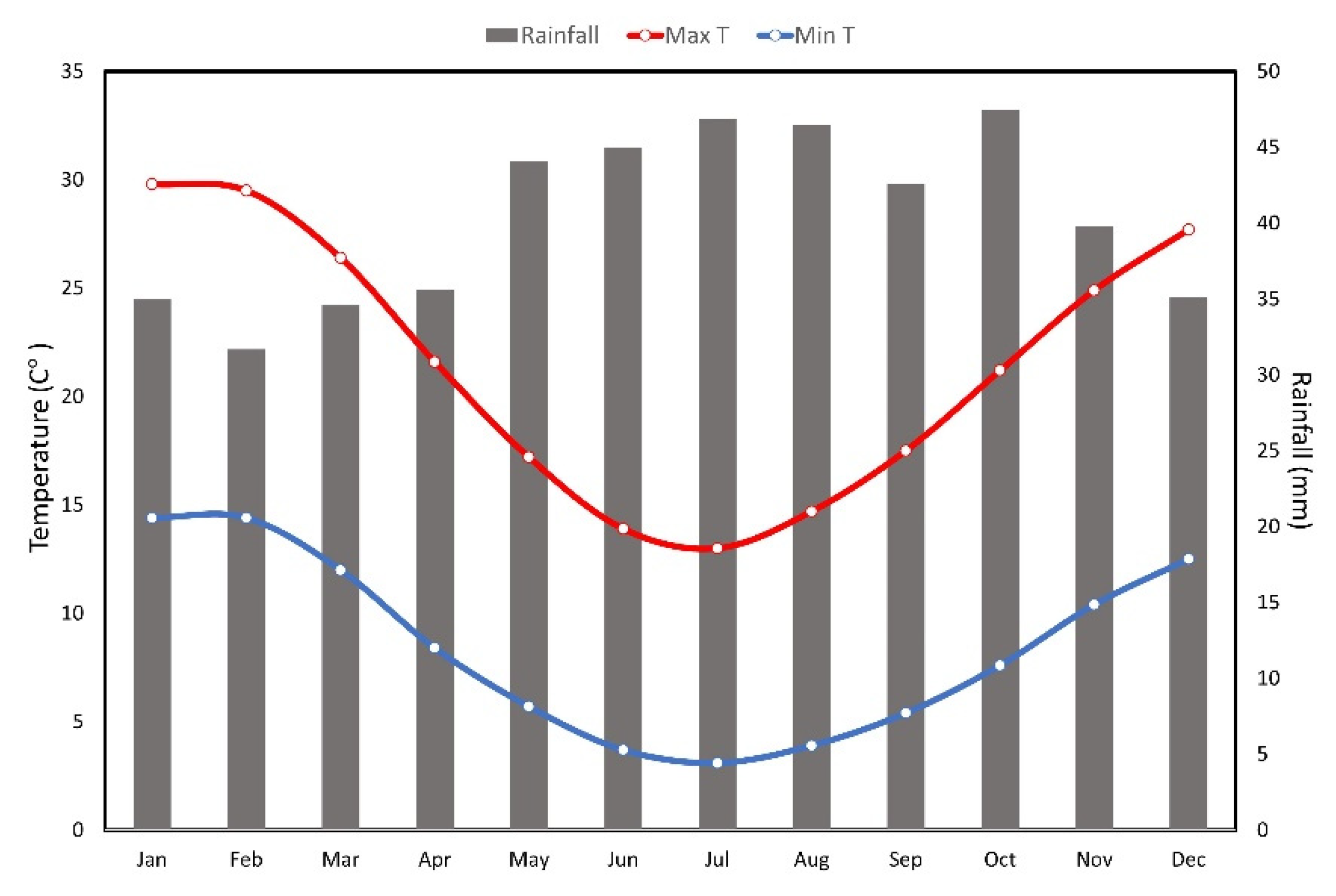
Figure 3.
(A) Concept of thresholding classification (optical approach). α and φ are the thresholds for NDVI and STR respectively, determined by an iterative thresholding method by minimizing within-class variance. Irrigated pixels are those with NDVI ≥ α and STR ≥ φ located within Sector 4. (B) Concept of thresholding classification (thermal approach). α and β are the thresholds for NDVI and Ts-Ta respectively, determined by an iterative thresholding method by minimizing within-class variance. Irrigated pixels are those with NDVI ≥ α and Ts-Ta ≤β in Sector 4.
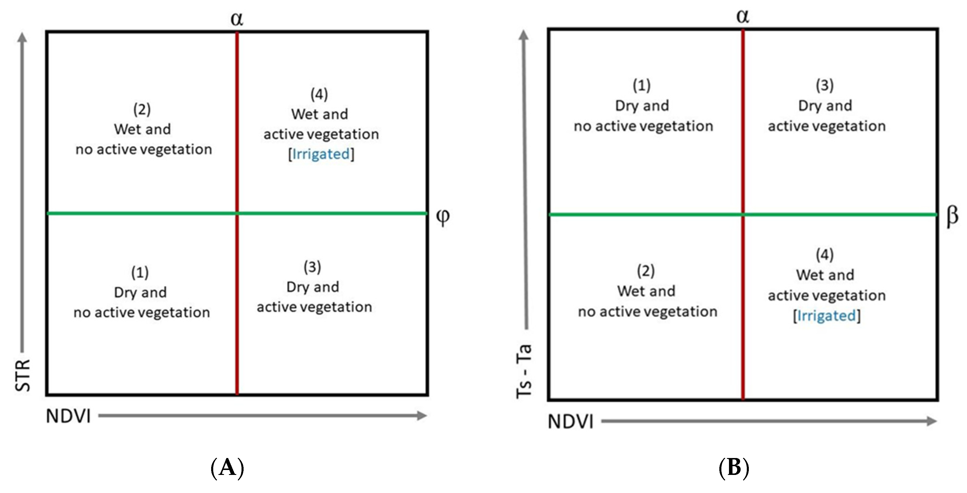
Figure 4.
Centroids showing the location of the farms in CGID used in the validation process. The background is the Landsat-8 images with bands 5/4/3 (displayed as a false colour composite image).
Figure 4.
Centroids showing the location of the farms in CGID used in the validation process. The background is the Landsat-8 images with bands 5/4/3 (displayed as a false colour composite image).
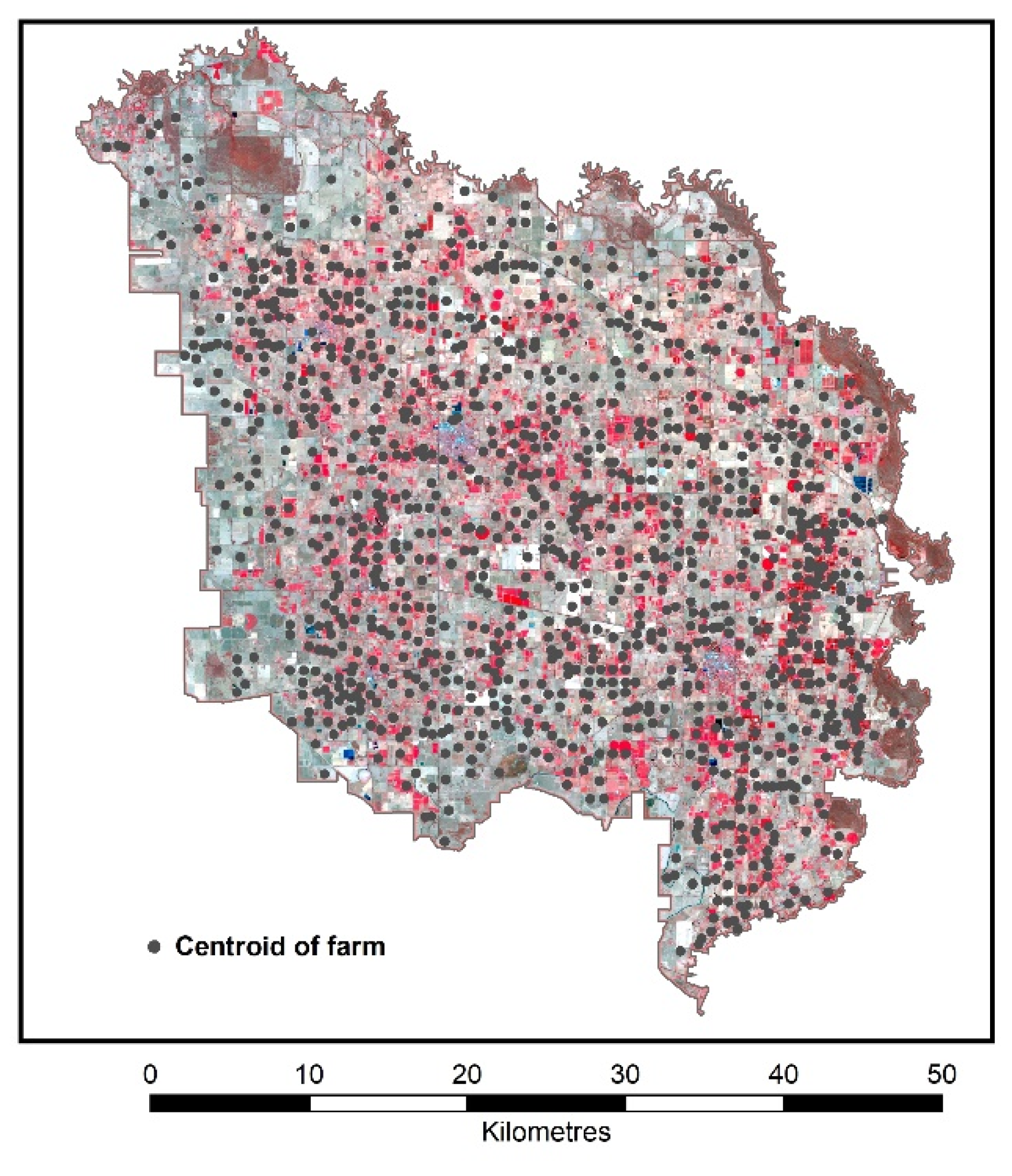
Figure 5.
Maps of individual input measures in CGID. (A) NDVI, (B) STR, (C) NWDI, (D) Ta, (E) Ts, and (F) Ts-Ta.
Figure 5.
Maps of individual input measures in CGID. (A) NDVI, (B) STR, (C) NWDI, (D) Ta, (E) Ts, and (F) Ts-Ta.
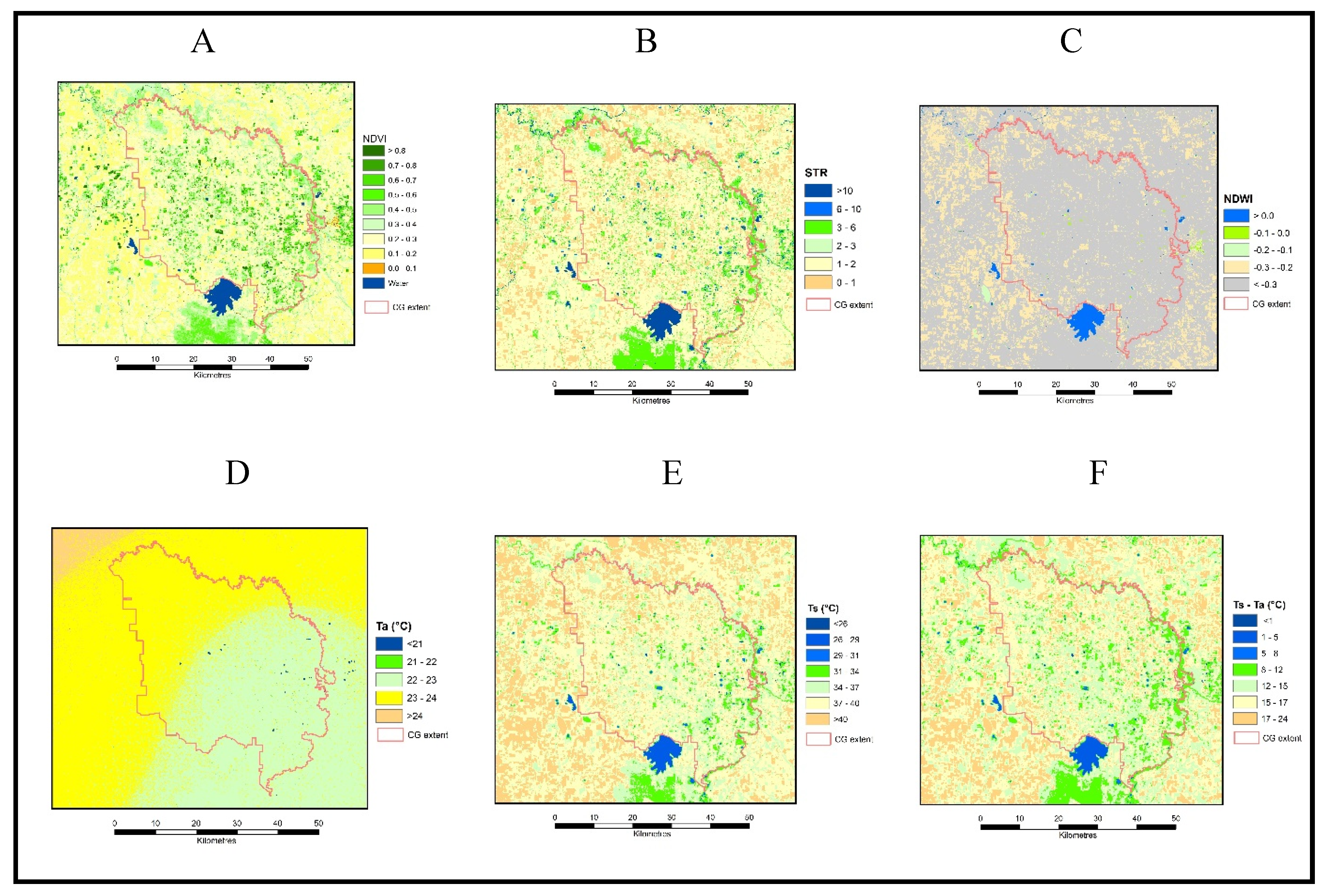
Figure 6.
Pixel identification based on thresholds. (A) Optical approach, and (B) Thermal approach of individual input measures in CGID. (Refer to Figure 3A,B for the descriptions of the four sectors, labelled here as 1-4).
Figure 6.
Pixel identification based on thresholds. (A) Optical approach, and (B) Thermal approach of individual input measures in CGID. (Refer to Figure 3A,B for the descriptions of the four sectors, labelled here as 1-4).
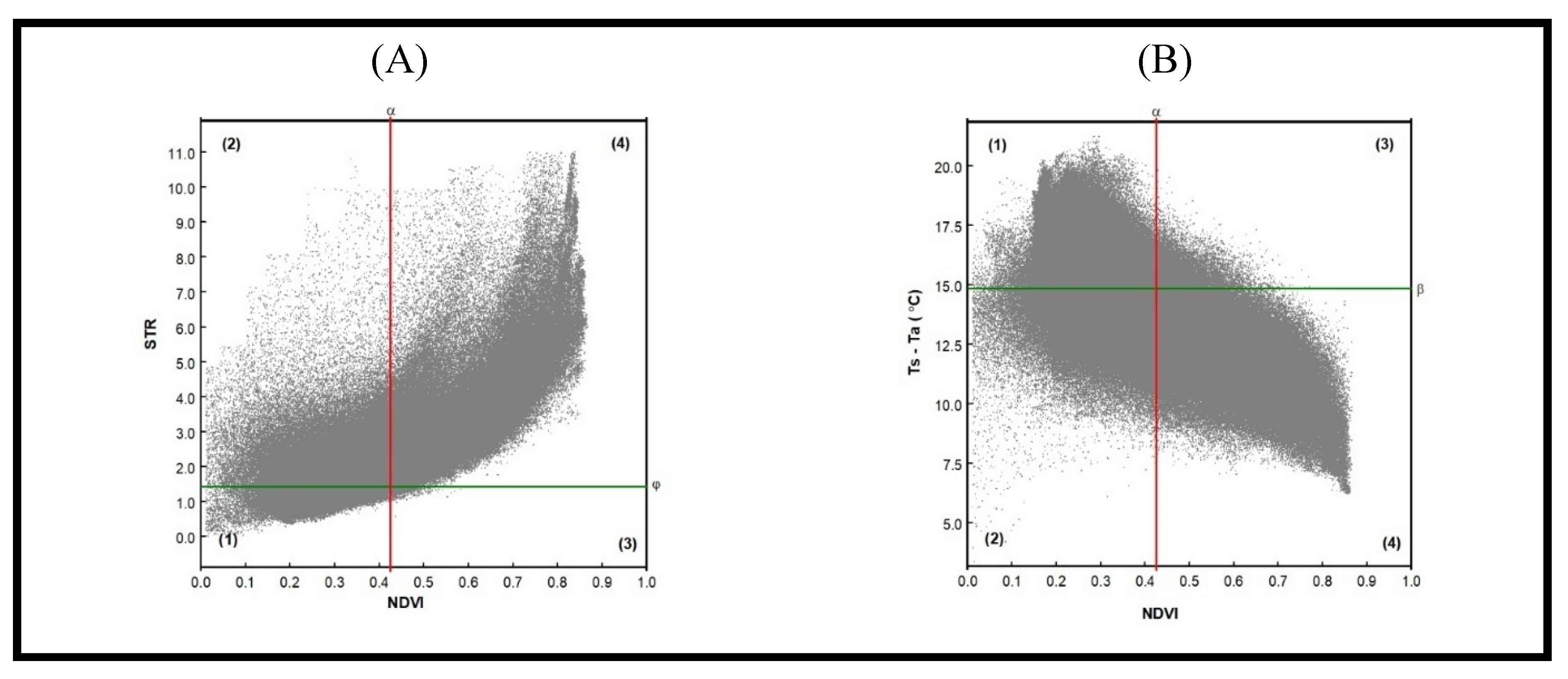
Figure 7.
Maps of irrigated landcover classes (Optical approach). (A) Pixel classes, (B) Irrigated landcover.
Figure 7.
Maps of irrigated landcover classes (Optical approach). (A) Pixel classes, (B) Irrigated landcover.
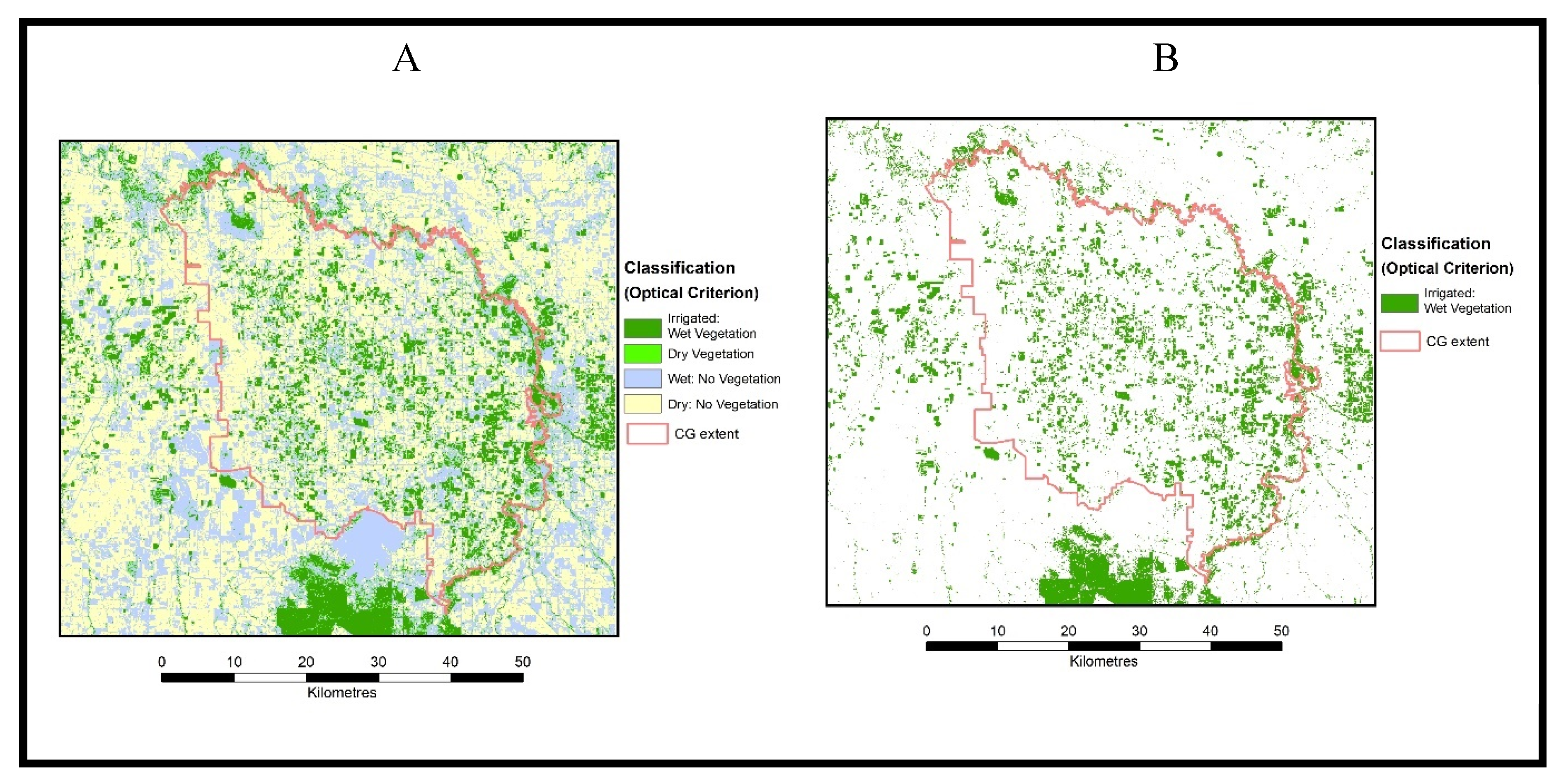
Figure 8.
Maps Maps of irrigated landcover classes (Thermal approach). (A) Pixel classes, (B) Irrigated landcover.
Figure 8.
Maps Maps of irrigated landcover classes (Thermal approach). (A) Pixel classes, (B) Irrigated landcover.
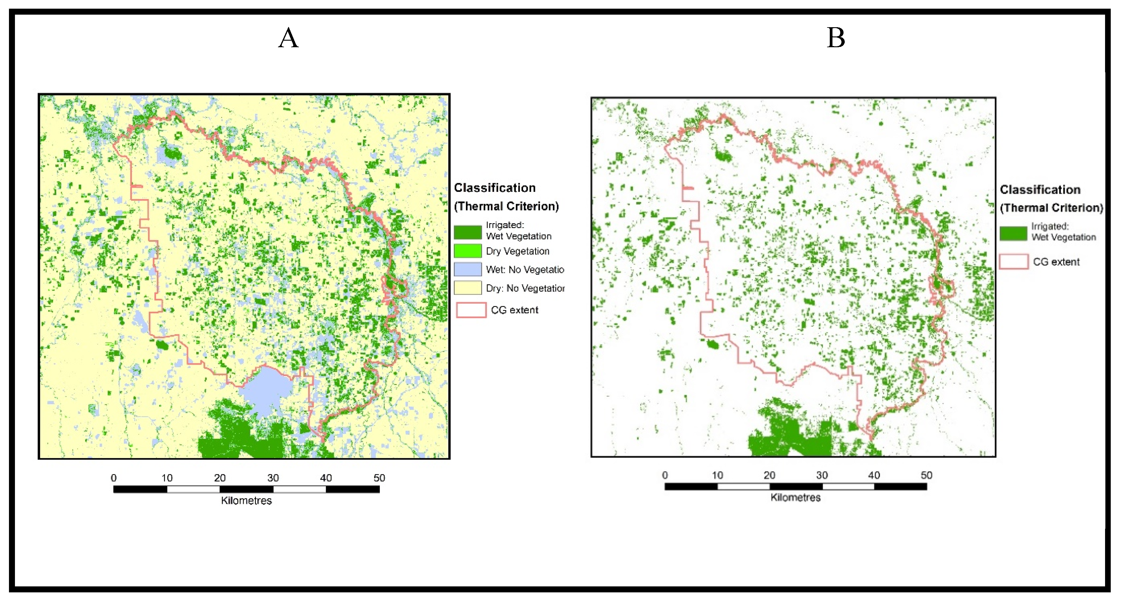

Table 1.
Soil moisture and drought indices based on reflectance in optical range.
| Index | Equation* | Reference |
| Vegetation Condition Index, VCI | Kogan, 1995 [26] | |
| Normalised Difference Water Index, NDWI | McFeeters, 1996 [27] | |
| Normalised Multiband Drought Index, NMDI | Wang and Qu, 2007 [28] | |
| Perpendicular Drought Index, PDI | Ghulam et al., 2007a [29] | |
| Modified Perpendicular Drought Index, MPDI | Ghulam et al. 2007b, [30] | |
| Modified Shortwave-infrared Perpendicular Water Stress index, MSPSI | Feng et al., 2013 [31] | |
| Distance Drought Index, DDI | Yang et al., 2008 [32] | |
| Visible and Shortwave-infrared Drought Index, VSDI | Zhang et al. 2013 [33] | |
| Shortwave Infrared Water Stress Index, SIWSI | Fensholt & Sandholt, 2003 [34] |
* NDVI, NDVImin, NDVImax: Smoothed weekly normalised difference vegetation index, its multi-year absolute maximum, and minimum, respectively; R: Reflectance; RGreen and RNIR: Reflectance of green and near-infrared spectral bands; M: Slope of the soil line on RRed and RNIR space; fv: Estimated vegetation cover; Rv: Coefficient taken as 0.5; and RSWIR: Reflectance of shortwave infrared spectral band.
Table 2.
Evaluation of irrigated landcover classification (Optical approach).
| (a) Occurrence (Optical approach) | |||||
| Classification | Reference* | Total | |||
| Irrigated | Non-Irrigated | ||||
| Irrigated | 451 | 8 | 459 | ||
| Non-Irrigated | 18 | 624 | 642 | ||
| Total | 469 | 632 | 1101 | ||
| * Classification according to water delivery records | |||||
| (b) Accuracy (Optical approach) | |||||
| Producer’s Accuracy % | User’s Accuracy % | ||||
| Irrigated | 96.2 | 98.3 | |||
| Non-Irrigated | 98.7 | 97.2 | |||
Overall accuracy = 97.6 %.
Table 3.
Evaluation of irrigated landcover classification (Thermal approach).
| (a) Occurrence (Thermal approach) | |||
| Classification | Reference* | Total | |
| Irrigated | Non-Irrigated | ||
| Irrigated | 404 | 55 | 459 |
| Non-Irrigated | 12 | 630 | 642 |
| Total | 416 | 685 | 1101 |
| * Classification according to water delivery records | |||
| (b) Accuracy (Thermal approach) | |||
| Producer’s Accuracy % | User’s Accuracy % | ||
| Irrigated | 97.1 | 88.0 | |
| Non-Irrigated | 92.0 | 98.12 | |
Overall accuracy = 93.9 %.
Disclaimer/Publisher’s Note: The statements, opinions and data contained in all publications are solely those of the individual author(s) and contributor(s) and not of MDPI and/or the editor(s). MDPI and/or the editor(s) disclaim responsibility for any injury to people or property resulting from any ideas, methods, instructions or products referred to in the content. |
© 2024 by the authors. Licensee MDPI, Basel, Switzerland. This article is an open access article distributed under the terms and conditions of the Creative Commons Attribution (CC BY) license (http://creativecommons.org/licenses/by/4.0/).
Copyright: This open access article is published under a Creative Commons CC BY 4.0 license, which permit the free download, distribution, and reuse, provided that the author and preprint are cited in any reuse.


