
Submitted:
04 March 2025
Posted:
04 March 2025
You are already at the latest version
Abstract
As urban expansion continues, understanding water resource dynamics in urban areas is crucial for sustainable city planning, flood risk mitigation, and long-term water security. Accurately identifying spatiotemporal changes in urban water resources is important for environmental monitoring and management. Geospatial and remote sensing tools and techniques enable efficient monitoring of water resources in rapidly growing cities, aiding in decision-making for sustainable urban planning. By leveraging advanced geospatial tools and techniques, this research examined spatiotemporal changes in 17 lakes within the rapidly expanding Dallas-Fort Worth (DFW) metropolitan area in the United States from 1984 to 2021, using the Global Surface Water (GSW) dataset via cloud-based remote sensing (Google Earth Engine, GEE) and non-cloud-based remote sensing (ArcGIS Pro). The research employed iso-cluster unsupervised classification and deep learning-supervised classification methods for land cover analysis. The study utilized ArcGIS Pro’s pre-trained deep learning model, based on the National Land Cover Database (NLCD), to classify Landsat images. A comparative analysis was conducted to statistically compare the classification outcomes of the Landsat/NLCD-ArcGIS Pro and GSW-GEE methods in estimating changes in urban lakes. The findings indicate that there is no statistically significant difference between the two datasets and methods. This suggests that both the Landsat/NLCD-ArcGIS Pro and GSW-GEE methods can effectively detect changes in lakes over space and time, although their accuracy may vary slightly depending on the specific lake and classification approach used. Moreover, the total surface area of all lakes estimated using the GSW-GEE method is slightly larger than that estimated using the Landsat-ArcGIS Pro method. Overall, this study highlights the importance of selecting the appropriate dataset and method for analyzing spatiotemporal changes in urban lake environments. The findings have practical implications for environmental researchers, managers, and policymakers involved in urban lake conservation and management.
Keywords:
Remote Sensing
; Global Surface Water Dataset
; Landsat Dataset
; ArcGIS Pro
; Google Earth Engine
; Dallas-Fort Worth
1. Introduction
Urban lakes play a significant role in providing a wide variety of ecosystem services that have an immediate and direct influence on human well-being, both in the present and in the future [1,2]. These ecosystem services include the production of agricultural goods, the management of fisheries, the control of flooding, the storage of water, and the creation of recreational opportunities [3]. Changes in the volume and location of a lake’s water across time and space can influence the provision of these services [4,5]. Therefore, to ensure both the sustainable management of water resources and sustainable urban development, it is vital to have a thorough understanding of spatiotemporal changes in urban lake-water extent. Water resource availability drives water infrastructure, large-scale water transfers between cities and urban areas, as well as the cost of potable water infrastructure and treatment [6,7]. This is particularly important as high rates of urbanization lead to over 1.5 billion more people living in cities, creating water availability issues for hundreds of millions to over a billion people worldwide. As a result, water resources are increasingly allocated to cities and other urban areas instead of agricultural regions [8,9]. This issue is especially important in densely populated urban areas like the Dallas-Fort Worth (DFW) metropolitan area, one of the fastest-growing regions in the United States (U.S.), which has a significant number of both artificial and natural lakes [10,11].
The DFW metropolitan area, which includes cities such as Dallas, Fort Worth, Arlington, Plano, and Irving, along with their surrounding suburbs, is ranked as the fourth-largest metropolitan area in the United States [12]. The area is recognized for its substantial lake-water coverage and humid subtropical climate. However, due to the rapid growth of the DFW metropolitan area in recent years, preserving the quantity and quality of lake water has become more difficult. While the dynamics of lake-water extent have become increasingly significant, only a few studies have explored the entire urban agglomeration. Most research has focused on imaging data for specific years, overlooking the temporary variations in lake-water extent. Therefore, it is necessary to have a clear understanding of the spatiotemporal changes in lake-water extent in the DFW metropolitan area [11,13]. Evaluating changes in lake-water extent over time and space using remote sensing (RS) data is a widely studied topic, particularly through Landsat image data due to its moderate spatial resolution (30–60 m) and long historical record [14,15,16,17,18]. RS efforts also play a major role in urban water management, being frequently used for integrated urban water resource management, flood risk evaluation, and urban water supply monitoring [19,20,21,22].
These studies highlight the significance of RS in understanding the evolving dynamics of surface water bodies and underscore its importance in providing valuable insights for effective management and conservation efforts. Most of these studies have primarily focused on the classification of satellite images that capture bodies of water, computationally intensive processes especially when analyzing large areas or numerous images. This process can also be prone to misclassification due to the varied spectral signatures emitted by water surfaces [23]. However, in recent years, researchers have attempted to address these challenges by developing reproducible techniques and datasets, such as the Joint Research Centre Global Surface Water dataset [24]. This dataset offers high temporal and spatial resolution, extensive validation, and the ability to automatically track spatial and temporal variations in water bodies efficiently. Additionally, it can be used by individuals without extensive coding skills on open-source, cloud-based RS platforms such as Google Earth Engine (GEE).
The Google Earth Engine (GEE) cloud-based remote sensing (RS) platform has recently become increasingly popular due to its ability to process large volumes of data and perform planetary-scale analysis [25]. In contrast, non-cloud-based RS platforms (e.g., ArcGIS) typically retrieve RS data from central data servers, which is then processed on local computers or servers [26,27,28]. Previous studies [27,28,29,30,31] suggest that non-cloud-based RS processing techniques can fall short of meeting the temporal requirements of dynamic monitoring. Conversely, cloud-based RS provides an alternative to this challenge by offering both a practical method for conducting RS computing and an effective data management service. To study the differences between cloud-based and non-cloud-based RS, this research aims to compare the effectiveness of cloud-based RS platforms with traditional RS techniques in capturing the spatiotemporal changes of lakes. The findings from this study will provide valuable insights into the potential benefits and limitations of cloud-based and non-cloud-based RS tools and technologies, informing future decisions about RS technology adoption and utilization. Thus, this study seeks to answer the following research questions:
- To what extent does the use of cloud-based RS platforms like GEE enhance the efficiency and precision of remote sensing applications by providing on-demand access to large datasets, advanced computing resources, and high-resolution imagery with planetary-scale analysis capabilities?
- How does the accuracy of non-cloud-based RS platforms like ArcGIS Pro compare to that of cloud-based RS platforms like GEE in estimating spatial and temporal changes in urban lakes?
Therefore, we hypothesized that:
- -
- H0: The change values for water bodies from 1984 to 2021, as well as over the five periods 1984–1994, 1994–2004, 2004–2014, and 2014–2021, using the Global Surface Water (GSW) dataset via GEE cloud-based RS and the Landsat dataset via non-cloud-based RS (ArcGIS Pro), do not differ significantly.
- -
- Ha: The change values for water bodies from 1984 to 2021, as well as over the five periods 1984–1994, 1994–2004, 2004–2014, and 2014–2021, using the Global Surface Water (GSW) dataset via GEE cloud-based RS and the Landsat dataset via non-cloud-based RS (ArcGIS Pro), differ significantly.
2. Materials and Methods
2.1. Study Area
We focused on lakes in the Dallas-Fort Worth (DFW) metropolitan area in Texas, USA (Figure 1). We used the 2016 HydroLAKES Database to obtain the most updated vector data of lake boundaries (https://www.hydrosheds.org/products/hydrolakes, accessed on June 10, 2022). The use of the HydroLAKES database ensures that the most recent and accurate data on lake boundaries is used in the analysis. The DFW area is full of natural and artificial lakes, but we prioritized lakes that have been frequently studied in the lake literature and vary in terms of watershed or socioeconomic context (e.g., population), making them vulnerable to land cover and land use change (LCLUC) (Table 1). The focus of this study is on the lakes within the DFW area, which include both natural and artificial lakes (Figure 1). The study prioritized lakes (Table 1) that have been frequently studied and vary in terms of watershed or socioeconomic context, making them vulnerable to LCLUC. The DFW area is an ideal location for studying lakes due to its abundance of natural and artificial water bodies. The study area holds great significance since it provides an opportunity to gain a deeper comprehension of the fluctuations in lakes over time and space within the DFW area, which can have far-reaching ecological and societal implications.
Table 1 provides characteristics of the 17 selected lakes within the DFW area, obtained from the 2016 HydroLAKES database. The table shows that the lakes vary greatly in area, with Lake Ray Hubbard being the largest at 79.89 km2 and Fishing Hole Lake being the smallest at 0.23 Km2. The Table also shows Lewisville Lake has the largest volume of 2581.62 Km3, while North Lake has the smallest volume of 29.6 km3. In terms of average depth, Grapevine Lake has the deepest average depth of 44.1 m, while Fishing Hole Lake has the shallowest average depth of 2 m. The results of this table are important as they provide an overview of the characteristics of the selected lakes and can be used as a basis for further analysis of the ecological and societal impacts of LCLUC in the DFW area.
2.2. Data Sources and Processing
Two datasets were utilized in the present study, namely, Landsat and one of Landsat’s derivative products: Joint Research Centre Global Surface Water (hereafter referred to as JRC/GSW) [24]. The Landsat satellite images used in the present study came from two different sources: Landsat 5 TM for the years 1984, 1994, and 2004 and Landsat 8 Operational Land Imager (OLI) for the years 2014 and 2021. The study utilized Google Earth Engine (hereafter referred to as GEE), a cloud-based platform that can analyze geospatial datasets and satellite imagery on a global scale, to extract Landsat 5 and 8 images. The satellite images for this study were chosen based on two criteria: the images must have less than 10% cloud cover, and the satellite image series must be available for an extended period [32,33]. The Landsat images were filtered by date and cloud cover less than 10%, and then the median of the images was calculated. For Landsat 8 OLI, images were extracted for the years 2022 and 2014, while for Landsat 5 TM, images were extracted for the years 2004, 1994, and 1984. Finally, the images were exported to Google Drive with a scale of 30 and in int16 format for further analysis.
The second dataset we used to extract spatiotemporal changes of water resources was JRC/GSW on the GEE platform. The JRC/GSW is a dataset created by the European Commission’s JRC that maps the extent of water bodies, such as lakes, rivers, and wetlands, on the Earth’s surface using satellite imagery. The dataset covers the entire globe and has a spatial resolution of 30 meters. The JRC/GSW dataset was created by analyzing images from the Landsat satellites, which have been collecting data on the Earth’s surface since the 1970s. The JRC/GSW uses advanced image processing techniques to identify and map water bodies, and the dataset is regularly updated to reflect changes in the Earth’s surface over time [24].
2.3. Detecting Spatiotemporal Variations
We analyzed the changes in lakes over time and space using two datasets and methods: JRC/GSW on the GEE and Landsat 5-8 on ArcGIS Pro, as follows:
2.3.1. The JRC/GSW Dataset and Google Earth Engine
We extracted the vector data (polygon) of the lakes for the years 1984, 1994, 2004, 2014, and 2021. The following steps were used as a methodology to extract spatiotemporal changes in lakes using the JRC/GSW dataset on the GEE. All these steps are done using a code developed on the GEE JavaScript API platform to perform the analysis and visualize the results on the map.
- -
- Step 1: A region of interest (ROI) is defined. In this case, it is the polygon of lakes that encompasses the study area of interest.
- -
- Step 2: The JRC/GSW dataset is loaded, and the “occurrence” band is selected.
- -
- Step 3: A water mask is created by selecting the “max_extent” band from the JRC/GSW and masking out the pixels with a value of 0.
- -
- Step 4: Lost water bodies are identified by selecting the “transition” band from the JRC/GSW and identifying pixels that have a value of 3 or 6, which indicate the transition from permanent or seasonal water to no water.
- -
- Step 5: Yearly water history is obtained for four years (1984, 1994, 2004, 2014, and 2021) using the JRC/GSW dataset. The “year” property is filtered to obtain the image for a specific year, and the “permanent” or “seasonal” water pixels are selected.
2.3.2. The Landsat Datasets and ArcGIS Pro
To estimate changes in lakes over space and time, we computed their areas using images from Landsat 5 TM and Landsat 8 OLI images in 1984 and 2021, as well as in the years 1994, 2004, and 2014. There are various supervised and unsupervised classification techniques available for image classification, each with its own advantages and disadvantages. In our study, we utilized an unsupervised and a supervised classification method as follows:
- -
- Step 1: Classifying land cover: To classify Landsat 5 TM images from 1984, 1994, and 2004, we used the iso cluster unsupervised classification method. Land cover classification is a complex task, and traditional methods may not capture its intricacies effectively. While deep learning (DL) models can learn complex semantics and yield superior results, creating and training these models can be challenging and time-consuming. To overcome this obstacle, we utilized pre-trained DL models in ArcGIS Pro, which have already been developed, tested, and verified by a panel of experts, to classify Landsat 8 OLI images from 2014 and 2021. These pre-trained DL models are designed to perform land cover classification on Landsat 8 imagery and are based on the National Land Cover Database (NLCD), which is one of the widely used datasets for land cover—land use change analysis in the United States of America [34,35].
- -
- Step 2: Cleaning up the classification: We first removed small, isolated areas that were classified as water but were not part of lakes. Some of these areas comprised tiny ponds or water bodies, while others were misclassified. These areas should not be included when calculating the lakes’ area. We then cleaned the image boundaries to eliminate pixelated, granular edges between values in each image.
- -
- Step 3: Computing lakes’ area over time: We determined the lakes’ areas in square kilometers from 1984 to 2021. To accomplish this, we selected the appropriate formula. The cell size parameters X and Y in Landsat images refer to the length and height of each pixel, respectively. In this case, each pixel on the map corresponds to an area of 30 units by 30 units in the real world, with the measurement being meters. To determine the area of each value in the image, we multiplied the pixel count by 900 to convert it to square meters. Then, we divided the result by 1,000, which represents the number of square meters in a square kilometer. The spatial and image analyses were performed utilizing the Spatial Analyst and Image Analyst tools in ArcGIS Pro 3.0.1 [36].
2.4. Comparative Analysis
We used descriptive statistics and inferential statistics for comparative statistical analysis. Descriptive statistics were used to summarize and describe the basic features of the datasets. Specifically, measures of central tendency (mean) and variability (standard deviation) were calculated to give an overview of the data. The minimum and maximum values were also reported to give a sense of the range of values in each dataset. Inferential statistics were then used to test whether there was a significant difference between the mean total change of the lakes in the datasets.
To compare the change values of each lake between the two methods/tools/datasets for the periods of 1984–2021 and each pair of consecutive years (1984–1994, 1994–2004, 2004–2014, and 2014–2021), we conducted a two-sample t-test to determine the statistical significance of the mean differences between the two methods/tools/datasets. Additionally, descriptive statistical parameters such as mean and standard deviation were calculated for the change values of each lake in both the JRC/GSW-GEE and Landsat/NLCD-ArcGIS Pro approaches. We employed the two-sample t-test to compare the change values between the two methods, as it is an appropriate statistical test for comparing the means of two groups, in this case, the mean total change values for each lake obtained from two different tools/datasets. The two-sample t-test is widely used and well-established, particularly for small sample sizes, as is the case here. Moreover, the t-test assumes normal distribution of data, which is reasonable for this type of data. Finally, the t-test provides a p-value, allowing for straightforward interpretation of the statistical significance of the observed differences in change values between these two geospatial tools and techniques [37,38].
3. Results
3.1. Spatiotemporal Variations in Lake Areas Based on JRC/GSW-GEE
The spatiotemporal variations in the surface area of various lakes (km2) between 1984 and 2021, obtained from the classification of the JRC/GSW dataset, are shown in Table 2 and Figure 2. Results indicate that there have been spatiotemporal variations in the surface area of the lakes between 1984 and 2021, based on the Landsat dataset. The lakes with the most changes have either significantly increased or decreased their water measurements over time. Lewisville Lake, for example, had the largest increase in its surface area, from 80.24 km2 in 1984 to 108.74 km2 in 2021, indicating a significant change in water levels over time. On the other hand, Lake Ray Hubbard had a small decrease in measurement from 83.96 km2 in 1984 to 83.52 km2 in 2021, indicating that the water level has been relatively stable over time. Grapevine Lake had a moderate increase in measurement from 22.09 km2 in 1984 to 28.17 km2 in 2021, suggesting that it has experienced some changes in its water level over time (Table 2).
Moreover, results indicated that the lakes with the most positive changes are Lewisville Lake, where the surface area increased from 80.24 km2 in 1984 to 108.74 km2 in 2021, an increase of 28.50 km2, Joe Pool Lake, where the surface area increased from 0.83 km2 in 1984 to 26.15 km2 in 2021, an increase of 25.32 km2, and Grapevine Lake, where the surface area increased from 22.09 km2 in 1984 to 28.17 km2 in 2021, an increase of 6.08 km2, respectively (Table 2 and Figure 2). On the other hand, lakes with the most negative changes are North Lake, where the surface area decreased from 2.94 km2 in 1984 to 1.14 km2 in 2021, a decrease of 1.80 km2, Fishing Hole Lake, where the surface area decreased from 1.04 km2 in 1984 to 0.30 km2 in 2021, a decrease of 0.74 km2, and Dallas Hunting and Fishing Club Lake, where the surface area decreased from 1.16 km2 in 1984 to 0.77 km2 in 2021, a decrease of 0.57 km2, respectively. In general, there was an increase of 63.00 km2 as the total size of lakes expanded from 350.89 km2 in 1984 to 413.89 km2 in 2021 (Table 2 and Figure 2).
Finally, the analysis of the most and least changes between years for each lake over the five periods between 1984–1994, 1994–2004, 2004–2014, and 2014–2021 (Table 3) showed that the lakes with the most changes are Joe Pool Lake with an increase of 23.95 km2, Benbrook Lake with an increase of 0.22 km2, Lake Ray Hubbard with a decrease of 12.52 km2, and Lake Ray Hubbard with an increase of 14.95 km2 for the periods of 1984–1994, 1994–2004, 2004–2014, and 2014–2021, respectively. On the other hand, the lakes with the least changes are Fishing Hole Lake with an increase of 0.02 km2, Fin and Feather Club Lake with a decrease of 0.74 km2, Dallas Hunting and Fishing Club Lake with a decrease of 0.09 km2, and Bachman Lake with an increase of 0.00 km2 for the periods of 1984–1994, 1994–2004, 2004–2014, and 2014–2021, respectively. Overall, the total surface area of all the lakes experienced the greatest positive change during the time frame of 2014-2021, with a recorded increase of 78.64 km2. Conversely, the greatest negative change was observed during the period of 2004-2014, with a decrease of 68.9 km2.
3.2. Spatiotemporal Variations in Lake Areas Based on Landsat/NLCD-ArcGIS Pro
Table 4 presents the spatiotemporal variations of the lakes, obtained from the Landsat dataset, from 1984 to 2021. Results indicated that there have been fluctuations in the water surface areas of these lakes over time. Some lakes have shown an increase in their water surface areas, while others have shown a decrease. For example, Joe Pool Lake showed a significant increase in its water surface area from 1984 to 2014, while North Lake showed a significant decrease during the same period. Overall, the total water surface area of all the lakes combined was highest in 1994 (416.22 km2) and lowest in 2014 (324.85 km2). However, the total water surface area in 2021 (403.49 km2) is slightly higher than that in 1984 (343.50 km2).
In addition, the lakes with the most positive changes from 1984 to 2021 are Lewisville Lake with a total increase of 31.19 km2, Joe Pool Lake with a total increase of 25.60 km2, and Grapevine Lake with a total increase of 4.16 km2, respectively. On the other hand, the lakes with the most negative changes from 1984 to 2021 are Lake Ray Hubbard with a total decrease of 2.08 km2, North Lake with a total decrease of 1.84 km2, and Dallas Hunting and Fishing Club Lake with a total decrease of 1.13 km2, respectively. In general, there was an increase of 59.99 km2 as the total size of lakes expanded from 343.50 km2 in 1984 to 403.49 km2 in 2021 (Table 4 and Figure 3).
Finally, the analysis of the most and least changes between years for each lake over the five periods between 1984–1994, 1994–2004, 2004–2014, and 2014–2021 (Table 5) showed that, for the period of 1984–1994, the lake with the most change is Lewisville Lake, with an increase of 33.68 km2, and the lake with the least change is Fishing Hole Lake, with an increase of only 0.03 km2. For the period of 1994–2004, the lake with the most change is Lewisville Lake, with a decrease of 6.48 km2, and the lake with the least change is Fishing Hole Lake, with an increase of only 0.01 km2. For the period of 2004–2014, the lake with the most change is Joe Pool Lake, with an increase of 1.97 km2, and the lake with the least change is Dallas Hunting and Fishing Club Lake, with a decrease of 1.12 km2. For the period of 2014–2021, the lake with the most change is Lewisville Lake, with an increase of 22.79 km2, and the lake with the least change is Dallas Hunting and Fishing Club Lake, with a decrease of 1.02 km2. In terms of the total change over the five-year period, Lewisville Lake has the most change, with an increase of 92.19 km2, and Dallas Hunting and Fishing Club Lake has the least change, with a decrease of 2.17 km2. In general, the total surface area of all the lakes experienced the highest growth (positive shift) during 2014-2021, with a rise of 109.38 km2. Conversely, the most significant decline (negative shift) in the surface area of all lakes was observed during the 2004-2014 period, with a decrease of 102.27 km2.
3.3. Comparative Analysis
Looking at the results in Table 2, Table 3, Table 4 and Table 5 and Figure 2 and Figure 3, we can compare the values obtained from the JRC/GSW-GEE and Landsat/NLCD-ArcGIS Pro approaches for measuring the surface area of each lake. In general, the values obtained from the two approaches are quite similar, indicating similar trends (Figure 4) between the two approaches, but there are some notable differences for certain lakes. For example, in the case of North Lake, the surface area obtained from JRC/GSW-GEE in 2014 consistently exceeded the values obtained from the Landsat/NLCD-ArcGIS Pro (Table 2 and Table 4, Figure 5). The JRC/GSW-GEE approach shows that North Lake has had the most negative change, while the Landsat/NLCD-ArcGIS Pro approach indicates that Lake Ray Hubbard has experienced the most negative change (Table 2 and Table 4). On the other hand, Joe Pool Lake has much lower values in the Landsat/NLCD-ArcGIS Pro approach than in the JRC/GSW-GEE approach, particularly in the early years of the study (Figure 6). In general, the total surface area of all lakes in the JRC/GSW-GEE approach (63.00 km2) is slightly greater than the total surface area of all lakes in the Landsat/NLCD-ArcGIS Pro approach (59.99 km2).
Table 6 presents descriptive statistics for the variables in the study area, which are the changes in surface area of the lakes over different time periods, as measured by the JRC/GSW-GEE and the Landsat/NLCD-ArcGIS Pro approaches. The results show that the mean changes in the surface area of the lakes are generally positive, indicating an overall increase in the surface area of the lakes over time. However, the standard deviation values are quite large, suggesting that there is significant variability in the changes in the surface area of the lakes across the study area. In addition, we can see that some time periods have higher skewness and kurtosis values, indicating that the distribution of changes in surface area of the lakes during those time periods is more skewed and has a higher peak than a normal distribution. For example, the changes in surface area of the lakes from 1994-2004 based on the JRC/GSW-GEE approach have a skewness of 3.08 and kurtosis of 9.4, suggesting that there may have been significant changes in surface area of the lakes during that time period. Overall, these descriptive statistics provide a summary of the distribution of changes in surface area of the lakes across the study area and can help us better understand the patterns and variability of these changes over time.
Table 7 shows the results of a two-sample t-test that compares the changes in the surface area of the lakes from 1984 to 2021 based on the JRC/GSW-GEE approach and the changes based on the Landsat/NLCD-ArcGIS Pro approach. Based on the results in Table 7, none of the t-values for any of the time periods analyzed are statistically significant, meaning that there is no significant difference between the changes in surface area of the lakes as measured by the JRC/GSW-GEE and the Landsat/NLCD-ArcGIS Pro approaches. Therefore, we can conclude that the two approaches provide similar estimates of the changes in surface area of the lakes over time. Overall, these results suggest that both datasets are valid sources of information for monitoring changes in the surface area of the lakes and can be used interchangeably to study spatiotemporal changes over time.
4. Discussion
This study used two datasets, JRC/GSW and Landsat 5 TM and Landsat 8 OLI, to estimate the changes in the size of various lakes using two different methods: GEE-based RS and ArcGIS-based RS. The study found that both datasets and methods can provide accurate estimates of changes in lakes, indicating the significance of both datasets and methods in identifying the spatial and temporal variations of lake area. Despite the fact that the JRC/GSW dataset combined with GEE-based RS offers benefits such as global coverage, high accuracy, and historical observations covering 32 years that increase the number of analyzed lakes and save time in spatial and image analysis, the Landsat combined with ArcGIS-based RS have their advantages, such as not requiring coding and the use of pre-trained DL models that enable timely spatial and image analysis.
We observed that the surface area measurements for most of the lakes are quite similar using both approaches. The three lakes with the greatest total change from 1984-2021 are the same in both methods, namely Lewisville Lake, Joe Pool Lake, and Grapevine Lake. These lakes are amongst the largest lakes in the study area and are, therefore, appropriate for both approaches. The JRC/GWS and Landsat datasets are based on Landsat images, which have a proven track record of successfully detecting changes in large water bodies, as reported in several studies [39,40,41,42]. However, the two approaches produced some different results in terms of the magnitude and direction of the changes. This is mainly because the JRC/GSW dataset utilizes Landsat 5, 7, and 8 [23,24] while the Landsat dataset, used in this study, only uses Landsat 5 and 8. Although each Landsat dataset has its own set of advantages and disadvantages, the use of Landsat 7 in combination with other Landsat data sources can lead to enhanced detection of water bodies due to its enhanced technical specifications [43,44].
In addition, we found significant differences between the two methods in assessing the top lakes with the least overall changes from 1984 to 2021. The JRC/GSW dataset indicates that North Lake has undergone the greatest negative change, while the Landsat dataset indicates that Lake Ray Hubbard has experienced the most negative change. This variation in the spatial and temporal changes of small lakes (e.g., North Lake) or lakes with minimal changes over time and space emphasizes that using more Landsat data sources yields more accurate results in assessing small water changes, despite Landsat datasets being inadequate for small water bodies in comparison to other satellites like Sentinel. These results are consistent with previous studies [42,45,46,47], which suggest that integrating Landsat imagery with historical maps or other satellite datasets (e.g., Sentinel, MODIS) produces superior outcomes in tracking the variations of small water bodies and other urban water resources.
Furthermore, we found that there was no statistical difference between two approaches in terms of their ability to accurately determine the total area of lakes over a period of 37 years (1984–2021) as well as the area changes for each decade (1984–1994, 1994–2004, 2004–2014, and 2014–2021). This indicates that both the JRC/GSW dataset and the Landsat dataset are capable of estimating changes in lakes over time and place, regardless of the type of RS technology used, whether cloud-based (GEE) or non-cloud-based (ArcGIS Pro). Although could-based RS platforms such as GEE have a wide range of benefits, such as faster processing times, non-cloud-based RS platforms like ArcGIS Pro can provide similar results within a reasonable time frame, especially if the user is not comfortable with coding. Besides, DL pre-trained models are provided in ArcGIS Pro for applications such as object identification, image segmentation, and image classification. These models have been trained on large datasets of satellite or aerial imagery and can be utilized in a conventional manner (using Spatial and Image Analyst Toolsets) or through pre-scripted Python codes to automatically identify and classify objects or features within satellite images. When compared to training a DL model from scratch, using DL pre-trained models in ArcGIS Pro can save both resources and time. Additionally, the use of pre-trained models can enhance the accuracy and dependability of deep learning tasks [48,49,50,51]. Furthermore, ArcGIS Pro can match GEE’s functionality using Python scripts, which gives it unique benefits in conjunction with cloud-based RS platforms like GEE. This means that for individuals looking for an integrated platform with the benefits of both GEE and ArcGIS, it is possible to utilize both platforms in their work [52,53,54,55]. The integration of cloud-based and non-cloud-based RS platforms could provide a more comprehensive and effective approach for monitoring and managing water resources, particularly urban water resources, in the future. Further research is needed to explore the potential of combining multiple RS datasets and platforms to improve the accuracy and reliability of lake area estimation.
5. Conclusions
This study assessed changes in 17 lakes located in the fast-growing metropolitan region of DFW, USA from 1984 to 2021 and was conducted by utilizing the JRC/GSW dataset through cloud-based RS on the GEE, as well as the Landsat dataset via non-cloud-based RS on ArcGIS Pro. The results showed that GEE-based and ArcGIS-based RS approaches are both effective in estimating changes in lake areas using two different datasets. In conclusion, this study indicates the effectiveness of both approaches. The study highlights the significance of both datasets and methodologies in identifying the spatial and temporal variations of the lake area, and it implies that the use of more Landsat data sources produces more accurate findings in assessing changes in small water bodies. In addition, the study demonstrates that the use of more Landsat data sources provides more accurate results in identifying spatial and temporal variations of the lake area. In addition, the findings of the study indicate that there is no statistical difference between the two methods in terms of their ability to accurately determine the total area of lakes over a period of 37 years. This points out that cloud-based RS platforms and non-cloud-based RS platforms are both capable of estimating changes in lakes over time and place.
Overall, the findings of this research offer important new perspectives on the merits and drawbacks of utilizing various RS methodologies and datasets for monitoring changes in the extent of urban lakes. The results of this research could have significant implications for environmental monitoring and management, regarding the management of water resources and the protection of their supplies. The combination of cloud-based and non-cloud-based RS platforms may prove to be the key to developing a method that is both more comprehensive and more efficient for coders and non-coders when studying the monitoring and management of water resources. It is necessary to conduct additional studies to investigate the possibilities of merging several remote sensing datasets and technologies to increase the accuracy and reliability of lake area estimation. We recommend three future research directions:
- -
- Combining RS datasets and methods: Combining multiple RS datasets and methods may improve lake area estimation accuracy and reliability, providing more water resources management data for urban water planners.
- -
- Developing integrated, easy-to-use RS tools: Non-cloud-based RS platforms like ArcGIS Pro with DL pre-trained models can produce similar results in a relatively short period of time, especially for non-coders. Cloud-based RS platforms like GEE offer faster processing times. A future study could build an integrated, user-friendly, and freely accessible RS system that has the merits of both the ArcGIS Pro and GEE platforms.
Author Contributions
Conceptualization, A.R.; methodology, A.R. and M.A.B.; software, A.R.; validation, A.R. and M.A.B.; formal analysis, A.R.; investigation, A.R.; resources, A.R.; data curation, A.R.; writing—original draft preparation, A.R.; writing—review and editing, M.A.B.; visualization, A.R.; supervision, A.R.; project administration, A.R. All authors have read and agreed to the published version of the manuscript.
Funding
This research received no external funding.
Data Availability Statement
All the data used in this study are publicly available and can be accessed through the following links: (1) Global Surface Water (GSW) dataset: https://global-surface-water.appspot.com/, and (2) Landsat datasets: https://developers.google.com/earth-engine/datasets/catalog/landsat.
Acknowledgments
The author would like to express sincere gratitude to Baylor University in Waco, Texas, USA for providing the necessary workspace and access to ArcGIS Pro software, which were instrumental in facilitating this research.
Conflicts of Interest
The authors declare no conflicts of interest.
References
- Grizzetti, B.; Liquete, C.; Pistocchi, A.; Vigiak, O.; Zulian, G.; Bouraoui, F.; Cardoso, A. C. Relationship Between Ecological Condition and Ecosystem Services in European Rivers, Lakes and Coastal Waters. Science of the Total Environment 2019, 671, 452–465. [Google Scholar] [CrossRef] [PubMed]
- Zhong, S.; Geng, Y.; Qian, Y.; Chen, W.; Pan, H. Analyzing ecosystem services of freshwater lakes and their driving forces: The case of Erhai Lake, China. Environ. Sci. Pollut. Res. 2019, 26, 10219–10229. [Google Scholar] [CrossRef] [PubMed]
- Deng, Y.; Jiang, W.; Tang, Z.; Li, J.; Lv, J.; Chen, Z.; Jia, K. Spatio-Temporal Change of Lake Water Extent in Wuhan Urban Agglomeration Based on Landsat Images from 1987 to 2015. Remote Sensing 2017, 9, 270. [Google Scholar] [CrossRef]
- Balkanlou, K. R.; Müller, B.; Cord, A. F.; Panahi, F.; Malekian, A.; Jafari, M.; Egli, L. Spatiotemporal Dynamics of Ecosystem Services Provision in a Degraded Ecosystem: A Systematic Assessment in the Lake Urmia Basin, Iran. Science of the Total Environment 2020, 716, 137100. [Google Scholar] [CrossRef]
- Zhang, Z.; Xia, F.; Yang, D.; Huo, J.; Wang, G.; Chen, H. Spatiotemporal characteristics in ecosystem service value and its interaction with human activities in Xinjiang, China. Ecol. Indic. 2020, 110, 105826. [Google Scholar] [CrossRef]
- Gleick, P. H. A Look at Twenty-First Century Water Resources Development. Water International 2000, 25, 127–138. [Google Scholar] [CrossRef]
- Metelka, T. Integrated urban water cycle modeling. In Integrated Urban Water Resources Management; Springer Netherlands: Dordrecht, 2006; pp. 51–58. [Google Scholar]
- McDonald, R.I.; Douglas, I.; Revenga, C.; Hale, R.; Grimm, N.; Grönwall, J.; Fekete, B. Global urban growth and the geography of water availability, quality, and delivery. Ambio 2011, 40, 437–446. [Google Scholar] [CrossRef]
- Bao, C.; Fang, C. L. Water Resources Flows Related to Urbanization in China: Challenges and Perspectives for Water Management and Urban Development. Water Resources Management 2012, 26, 531–552. [Google Scholar] [CrossRef]
- Atkinson, S. F.; Lake, M. C. Prioritizing Riparian Corridors for Ecosystem Restoration in Urbanizing Watersheds. PeerJ 2020, 8, e8174. [Google Scholar] [CrossRef]
- Li, S. Mapping Urban Growth of Dallas-Fort Worth Metropolitan Area from 1984 to 2019 Using Landsat Data. M.Sc. Thesis, Texas Tech University, Lubbock, TX, USA, December 2020. [Google Scholar]
- Nostikasari, D. Representations of everyday travel experiences: Case study of the Dallas-Fort Worth Metropolitan Area. Transp. Policy 2015, 44, 96–107. [Google Scholar] [CrossRef]
- Homè, A.; Batcha, R. Snowmelt Flood Mapping and Land Surface Short-Term Dynamics Assessment in a “Before-During-After” Scenario Based on Radar and Optical Satellite Imagery: Case Study Around the Lewisville Lake (Dallas/Fort Worth Metropolitan, Texas, USA). Advances in Remote Sensing 2023, 12, 1–28. [Google Scholar] [CrossRef]
- Kuhn, C.; de Matos Valerio, A.; Ward, N.; Loken, L.; Sawakuchi, H.O.; Kampel, M.; Butman, D. Performance of Landsat-8 and Sentinel-2 surface reflectance products for river remote sensing retrievals of chlorophyll-a and turbidity. Remote Sens. Environ. 2019, 224, 104–118. [Google Scholar] [CrossRef]
- Li, X.; Ling, F.; Foody, G.M.; Boyd, D.S.; Jiang, L.; Zhang, Y.; Du, Y. Monitoring high spatiotemporal water dynamics by fusing MODIS, Landsat, water occurrence data, and DEM. Remote Sens. Environ. 2021, 265, 112680. [Google Scholar] [CrossRef]
- Mueller, N.; Lewis, A.; Roberts, D.; Ring, S.; Melrose, R.; Sixsmith, J.; Ip, A. Water observations from space: Mapping surface water from 25 years of Landsat imagery across Australia. Remote Sens. Environ. 2016, 174, 341–352. [Google Scholar] [CrossRef]
- Song, K.; Liu, G.; Wang, Q.; Wen, Z.; Lyu, L.; Du, Y.; Fang, C. Quantification of lake clarity in China using Landsat OLI imagery data. Remote Sens. Environ. 2020, 243, 111800. [Google Scholar] [CrossRef]
- Tulbure, M.G.; Broich, M.; Stehman, S.V.; Kommareddy, A. Surface water extent dynamics from three decades of seasonally continuous Landsat time series at subcontinental scale in a semi-arid region. Remote Sens. Environ. 2016, 178, 142–157. [Google Scholar] [CrossRef]
- Masser, I. Managing our urban future: The role of remote sensing and geographic information systems. Habitat Int. 2001, 25, 503–512. [Google Scholar] [CrossRef]
- McKinney, D.C.; Cai, X. Linking GIS and water resources management models: An object-oriented method. Environ. Model. Softw. 2002, 17, 413–425. [Google Scholar] [CrossRef]
- Wang, X.; Xie, H. A review on applications of remote sensing and geographic information systems (GIS) in water resources and flood risk management. Water 2018, 10, 608. [Google Scholar] [CrossRef]
- Sharma, S.K. Role of remote sensing and GIS in integrated water resources management (IWRM). In Ground Water Development—Issues and Sustainable Solutions; [Publisher]: [Location], 2019; pp. 211–227. [Google Scholar]
- Busker, T.; de Roo, A.; Gelati, E.; Schwatke, C.; Adamovic, M.; Bisselink, B.; Cottam, A. A Global Lake and Reservoir Volume Analysis Using a Surface Water Dataset and Satellite Altimetry. Hydrology and Earth System Sciences 2019, 23, 669–690. [Google Scholar] [CrossRef]
- Pekel, J.F.; Cottam, A.; Gorelick, N.; Belward, A.S. High-resolution mapping of global surface water and its long-term changes. Nature 2016, 540, 418–422. [Google Scholar] [CrossRef] [PubMed]
- Gorelick, N.; Hancher, M.; Dixon, M.; Ilyushchenko, S.; Thau, D.; Moore, R. Google Earth Engine: Planetary-Scale Geospatial Analysis for Everyone. Remote Sensing of Environment 2017, 202, 18–27. [Google Scholar] [CrossRef]
- Barsai, G. Getting to Know ArcGIS PRO. Photogrammetric Engineering & Remote Sensing 2018, 84, 181–182. [Google Scholar] [CrossRef]
- Dube, T.; Gumindoga, W.; Chawira, M. Detection of Land Cover Changes Around Lake Mutirikwi, Zimbabwe, Based on Traditional Remote Sensing Image Classification Techniques. African Journal of Aquatic Science 2014, 39, 89–95. [Google Scholar] [CrossRef]
- Saltus, C.L.; Reif, M.K.; Johansen, R.A. WaterQuality for ArcGIS Pro Toolbox: User’s Guide; Engineer Research and Development Center (US): Vicksburg, MS, USA, 2022. [Google Scholar]
- Wang, P.; Wang, J.; Chen, Y.; Ni, G. Rapid processing of remote sensing images based on cloud computing. Future Gener. Comput. Syst. 2013, 29, 1963–1968. [Google Scholar] [CrossRef]
- Zhang, Z.; Zhang, M.; Gong, J.; Hu, X.; Xiong, H.; Zhou, H.; Cao, Z. LuoJiaAI: A cloud-based artificial intelligence platform for remote sensing image interpretation. Geo-Spat. Inf. Sci.
- Zou, Q. Research on cloud computing for disaster monitoring using massive remote sensing data. In Proceedings of the 2017 IEEE 2nd International Conference on Cloud Computing and Big Data Analysis (ICCCBDA); IEEE; 2017; pp. 29–33. [Google Scholar]
- Chopade, M. R.; Mahajan, S.; Chaube, N. Assessment of Land Use, Land Cover Change in the Mangrove Forest of Ghogha Area, Gulf of Khambhat, Gujarat. Expert Systems with Applications 2023, 212, 118839. [Google Scholar] [CrossRef]
- Sun, Z.; Ma, R.; Wang, Y. Using Landsat data to determine land use changes in Datong Basin, China. Environ. Geol. 2009, 57, 1825–1837. [Google Scholar] [CrossRef]
- Homer, C.; Dewitz, J.; Jin, S.; Xian, G.; Costello, C.; Danielson, P.; Riitters, K. Conterminous United States land cover change patterns 2001–2016 from the 2016 national land cover database. ISPRS J. Photogramm. Remote Sens. 2020, 162, 184–199. [Google Scholar] [CrossRef]
- Wickham, J.; Stehman, S.V.; Sorenson, D.G.; Gass, L.; Dewitz, J.A. Thematic accuracy assessment of the NLCD 2016 land cover for the conterminous United States. Remote Sens. Environ. 2021, 257, 112357. [Google Scholar] [CrossRef]
- ESRI. ArcGIS Pro: Release 3.0.1. Environmental Systems Research Institute: Redlands, CA, USA, 2022.
- Noguchi, K.; Konietschke, F.; Marmolejo-Ramos, F.; Pauly, M. Permutation tests are robust and powerful at 0.5% and 5% significance levels. Behav. Res. Methods 2021, 53, 2712–2724. [Google Scholar] [CrossRef]
- Walters, W.H. Survey design, sampling, and significance testing: Key issues. J. Acad. Librariansh. 2021, 47, 102344. [Google Scholar] [CrossRef]
- Halabisky, M.; Moskal, L. M.; Gillespie, A.; Hannam, M. Reconstructing Semi-Arid Wetland Surface Water Dynamics Through Spectral Mixture Analysis of a Time Series of Landsat Satellite Images (1984–2011). Remote Sensing of Environment 2016, 177, 171–183. [Google Scholar] [CrossRef]
- Schaffer-Smith, D.; Swenson, J.J.; Barbaree, B.; Reiter, M.E. Three decades of Landsat-derived spring surface water dynamics in an agricultural wetland mosaic: Implications for migratory shorebirds. Remote Sens. Environ. 2017, 193, 180–192. [Google Scholar] [CrossRef] [PubMed]
- Wen, Z.; Wang, Q.; Liu, G.; Jacinthe, P.A.; Wang, X.; Lyu, L.; Song, K. Remote sensing of total suspended matter concentration in lakes across China using Landsat images and Google Earth Engine. ISPRS J. Photogramm. Remote Sens. 2022, 187, 61–78. [Google Scholar] [CrossRef]
- Yang, S.; Wan, R.; Yang, G.; Li, B.; Dong, L. Combining historical maps and Landsat images to delineate the centennial-scale changes of lake wetlands in Taihu Lake Basin, China. J. Environ. Manag. 2023, 329, 117110. [Google Scholar] [CrossRef]
- King, M.D.; Platnick, S. The Earth Observing System (EOS). In Comprehensive Remote Sensing; Liang, S., Ed.; Elsevier: 2018; pp. 7–26.
- Olmanson, L.G.; Brezonik, P.L.; Finlay, J.C.; Bauer, M.E. Comparison of Landsat 8 and Landsat 7 for regional measurements of CDOM and water clarity in lakes. Remote Sens. Environ. 2016, 185, 119–128. [Google Scholar] [CrossRef]
- Deliry, S. I.; Avdan, Z. Y.; Avdan, U. Extracting Urban Impervious Surfaces from Sentinel-2 and Landsat-8 Satellite Data for Urban Planning and Environmental Management. Environmental Science and Pollution Research 2021, 28, 6572–6586. [Google Scholar] [CrossRef] [PubMed]
- Chang, L.; Cheng, L.; Huang, C.; Qin, S.; Fu, C.; Li, S. Extracting Urban Water Bodies from Landsat Imagery Based on mNDWI and HSV Transformation. Remote Sensing 2022, 14, 5785. [Google Scholar] [CrossRef]
- Li, X.; Jia, X.; Yin, Z.; Du, Y.; Ling, F. Integrating MODIS and Landsat imagery to monitor the small water area variations of reservoirs. Sci. Remote Sens. 2022, 5, 100045. [Google Scholar] [CrossRef]
- Agapiou, A.; Vionis, A.; Papantoniou, G. Detection of Archaeological Surface Ceramics Using Deep Learning Image-Based Methods and Very High-Resolution UAV Imageries. Land 2021, 10, 1365. [Google Scholar] [CrossRef]
- Arnold, C. R. Locating Low Head Dams Using a Deep Learning Model in ArcGIS Pro with Aerial Imagery. Unpublished work.
- O’Neill, F.; Lasko, K.; Sava, E. Snow-Covered Region Improvements to a Support Vector Machine-Based Semi-Automated Land Cover Mapping Decision Support Tool; Engineer Research and Development Center (ERDC), U.S. Army Corps of Engineers: Vicksburg, MS, USA, 2022. [Google Scholar]
- Trevisan, J.; Migeon, S. Détections Automatiques de Structures Géomorphologiques Sous-Marines en Deep Learning avec ArcGIS Pro? In Le Géo Évènement SIG 2022; 22. 20 October.
- Cohen, S.; Peter, B. G.; Haag, A.; Munasinghe, D.; Moragoda, N.; Narayanan, A.; May, S. Sensitivity of Remote Sensing Floodwater Depth Calculation to Boundary Filtering and Digital Elevation Model Selections. Remote Sensing 2022, 14, 5313. [Google Scholar] [CrossRef]
- McClain, B.P. Python for Geospatial Data Analysis; O’Reilly Media, Inc.: 2022.
- Odion, D.; Shoji, K.; Evangelista, R.; Gajardo, J.; Motmans, T.; Defraeye, T.; Onwude, D. A GIS-based interactive map enabling data-driven decision-making in Nigeria’s food supply chain. MethodsX 2023, 10, 102047. [Google Scholar] [CrossRef] [PubMed]
- Smith, R.E. Flood Warning: A Generalized Approach to Forecast the Impacts of Flooding Events Using ArcGIS Pro, QGIS, and Python. M.Sc. Thesis, Brigham Young University, Provo, UT, USA, 2022. [Google Scholar]
Figure 1.
Location of the selected lakes in Dallas-Fort Worth, State of Texas, USA.
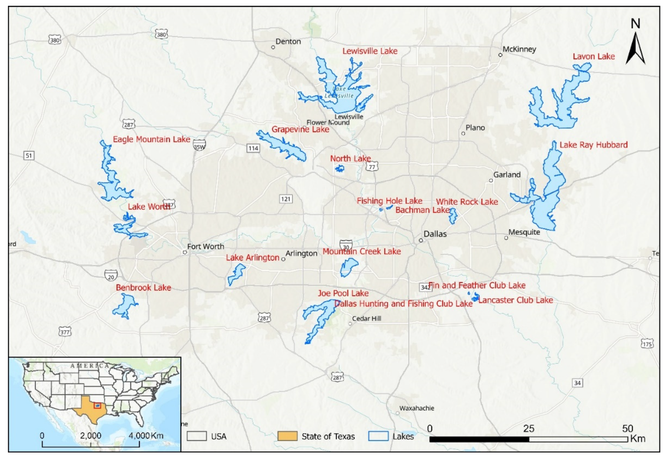
Figure 2.
Spatiotemporal variations of lakes, obtained from the JRC/GSW dataset, from 1984–2021.
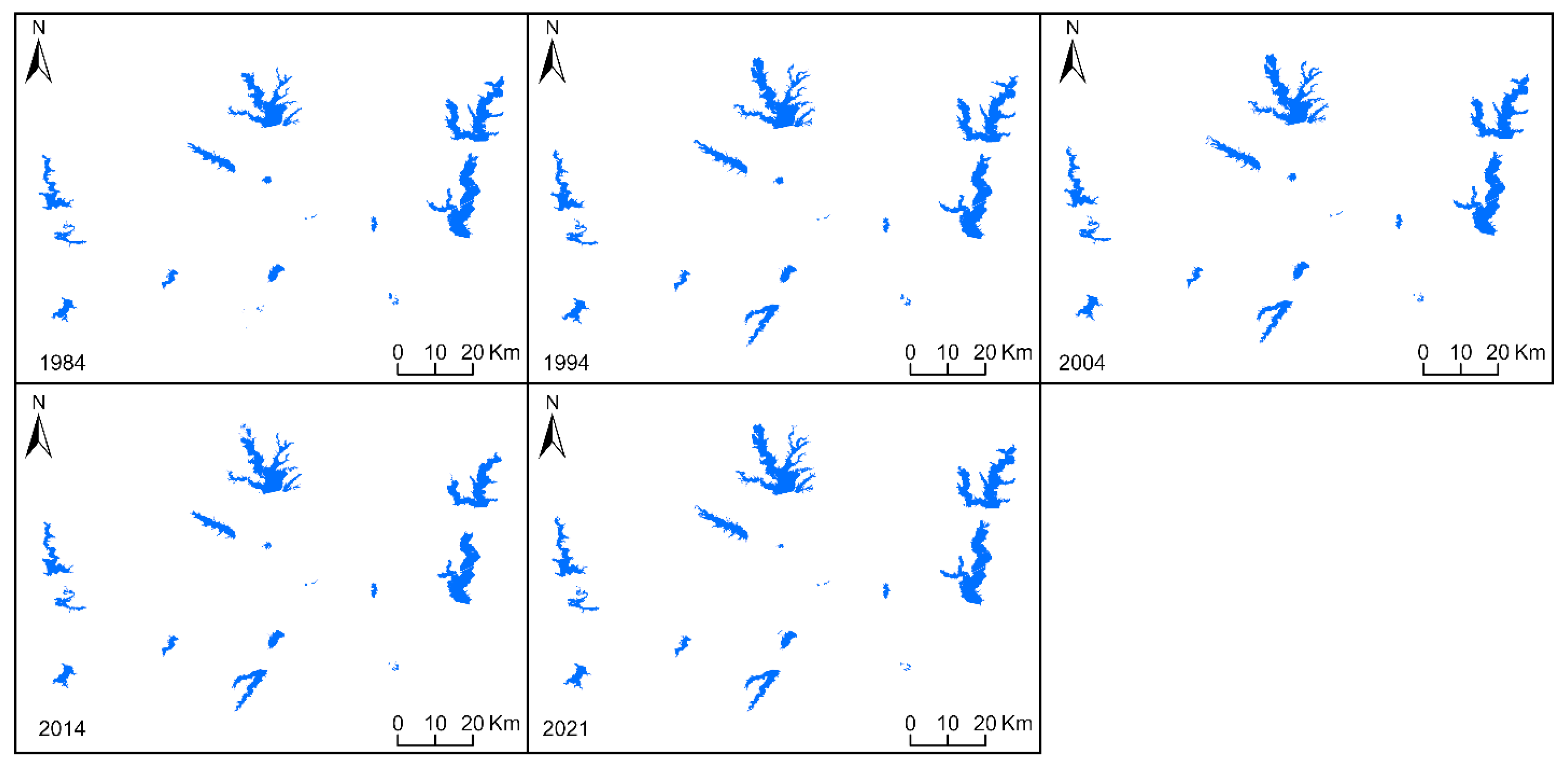
Figure 3.
Spatiotemporal variations of lakes, obtained from the Landsat, from 1984–2021.
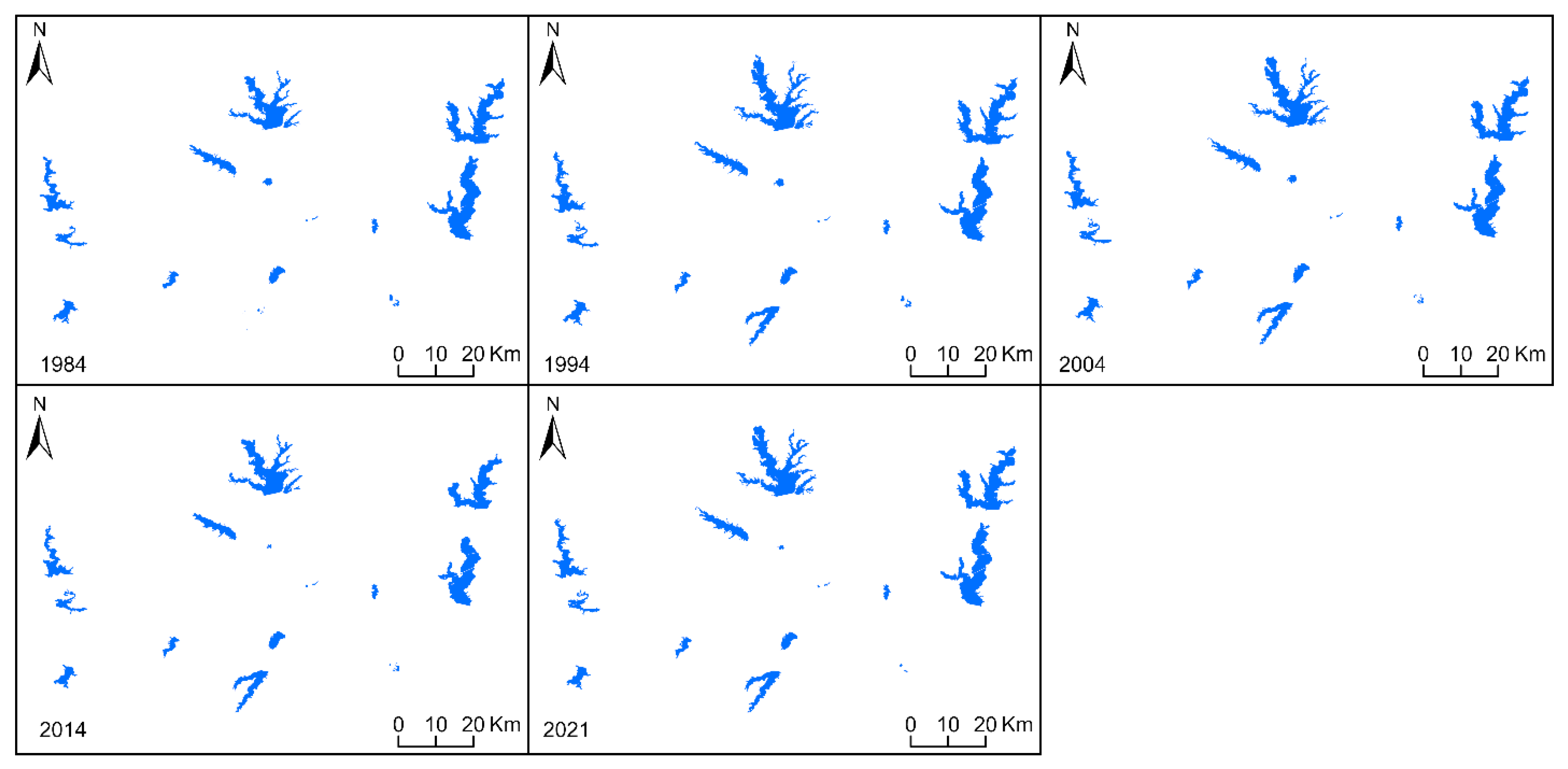
Figure 4.
Spatiotemporal trends of changes in lakes, obtained from the JRC/GSW-GEE and the Landsat/NLCD-ArcGIS Pro approaches, from 1984–2021.
Figure 4.
Spatiotemporal trends of changes in lakes, obtained from the JRC/GSW-GEE and the Landsat/NLCD-ArcGIS Pro approaches, from 1984–2021.
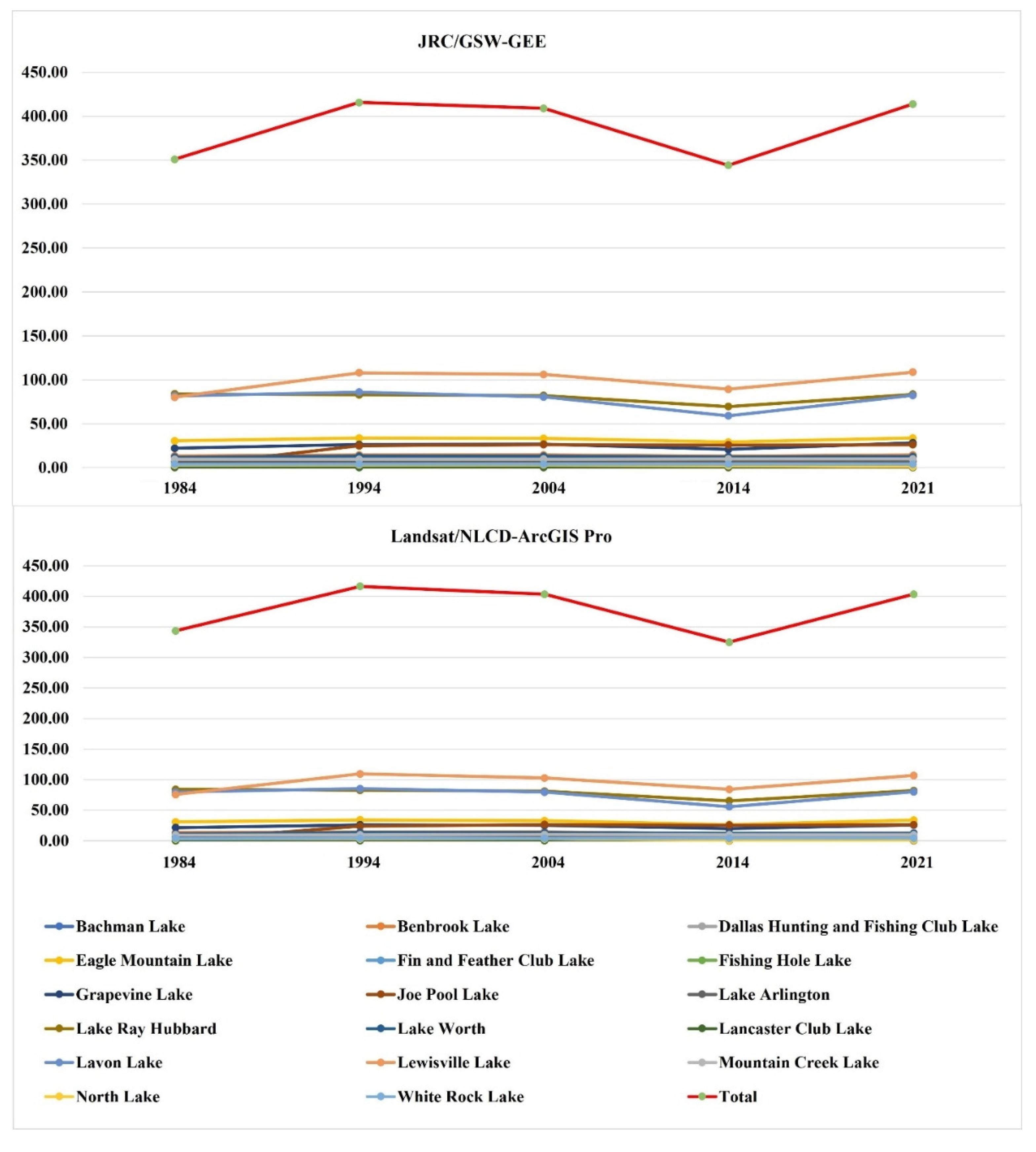
Figure 5.
Spatiotemporal variations of North Lake, obtained from the JRC/GSW-GEE (right) and the Landsat/NLCD-ArcGIS Pro (left) approaches, from 1984–2021.
Figure 5.
Spatiotemporal variations of North Lake, obtained from the JRC/GSW-GEE (right) and the Landsat/NLCD-ArcGIS Pro (left) approaches, from 1984–2021.
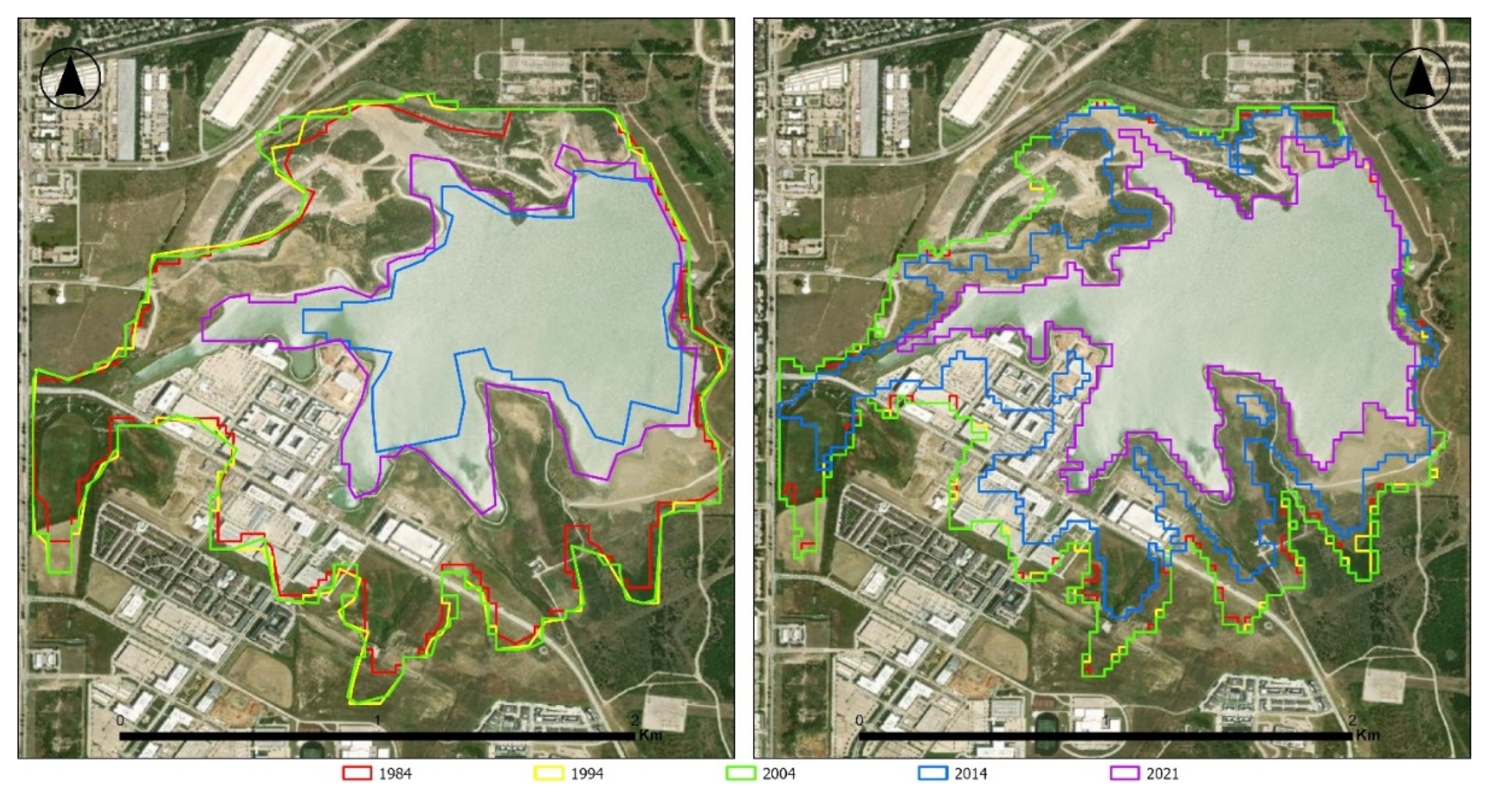
Figure 6.
Spatiotemporal variations of Joe Pool Lake, obtained from the JRC/GSW-GEE (right) and the Landsat/NLCD-ArcGIS Pro (left) approaches, from 1984–2021.
Figure 6.
Spatiotemporal variations of Joe Pool Lake, obtained from the JRC/GSW-GEE (right) and the Landsat/NLCD-ArcGIS Pro (left) approaches, from 1984–2021.
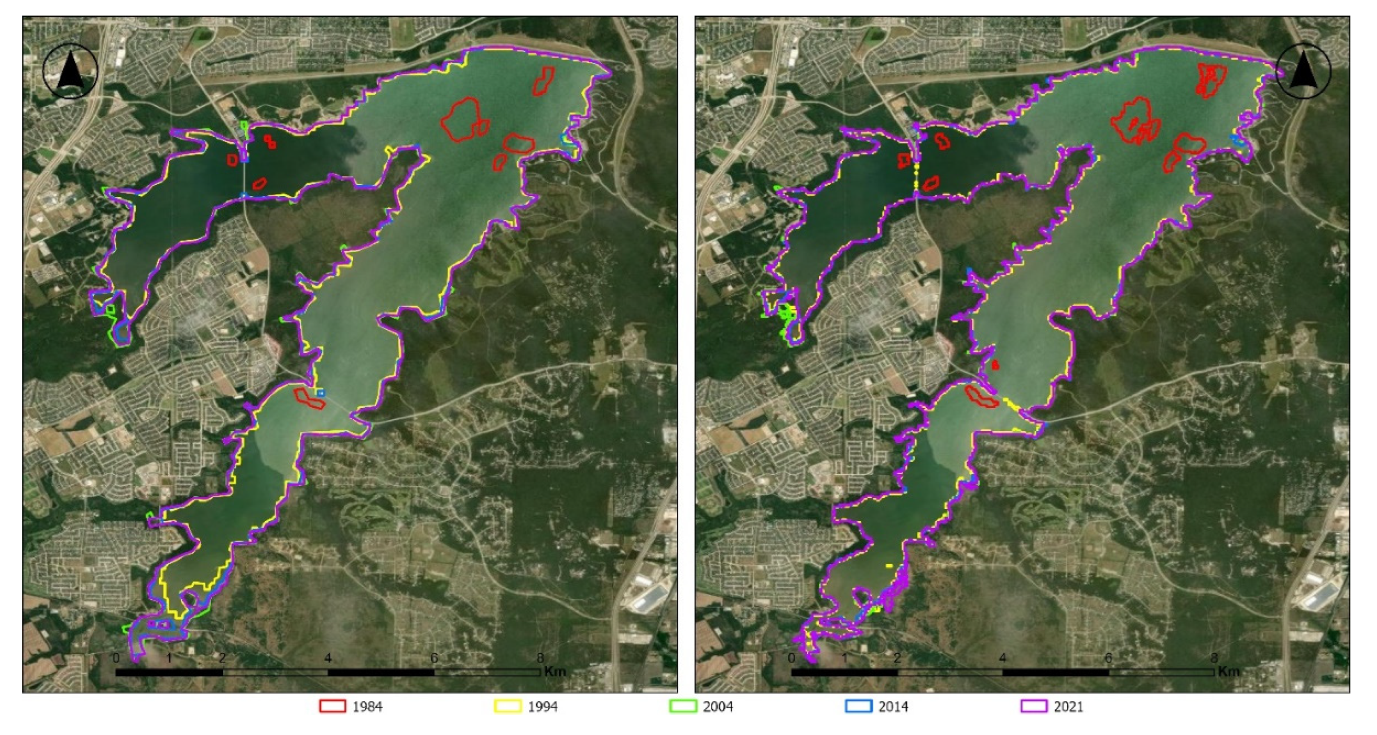

Table 1.
Characteristics of lakes defined by HydroLAKES database.
| Lake Name | Area (km2) | Volume (km3) | Average Depth (m) | Elevation (m) | Longitude | Latitude |
|---|---|---|---|---|---|---|
| Lake Ray Hubbard | 79.89 | 719.9 | 9 | 135 | -96.50 | 32.80 |
| Lavon Lake | 73.19 | 1153.01 | 16.6 | 151 | -96.47 | 33.03 |
| Lewisville Lake | 68.6 | 2581.62 | 39.2 | 157 | -96.97 | 33.07 |
| Eagle Mountain Lake | 29.07 | 839.2 | 28.9 | 200 | -97.50 | 32.87 |
| Joe Pool Lake | 23.53 | 792.5 | 33.7 | 160 | -96.99 | 32.64 |
| Grapevine Lake | 21.22 | 936 | 44.1 | 165 | -97.06 | 32.97 |
| Benbrook Lake | 12.12 | 505.7 | 41.7 | 213 | -97.46 | 32.65 |
| Lake Worth | 11.06 | 118.7 | 10.7 | 184 | -97.42 | 32.79 |
| Mountain Creek Lake | 8.98 | 87.4 | 9.7 | 143 | -96.94 | 32.73 |
| Lake Arlington | 6.51 | 127.7 | 19.6 | 170 | -97.19 | 32.72 |
| White Rock Lake | 3.9 | 48.6 | 12.5 | 143 | -96.73 | 32.82 |
| North Lake | 2.64 | 29.6 | 11.2 | 157 | -96.97 | 32.94 |
| Dallas Hunting and Fishing Club Lake | 1 | 2.77 | 2.8 | 121 | -96.67 | 32.64 |
| Bachman Lake | 0.37 | 0.89 | 2.4 | 138 | -96.87 | 32.85 |
| Lancaster Club Lake | 0.24 | 0.6 | 2.5 | 121 | -96.67 | 32.64 |
| Fishing Hole Lake | 0.23 | 0.45 | 2 | 130 | -96.89 | 32.85 |
| Fin and Feather Club Lake | 0.14 | 0.28 | 2 | 120 | -96.69 | 32.66 |
| Total | 342.69 | 7944.92 | - | - | - | - |
Table 2.
Spatiotemporal variations of the lakes, obtained from the JRC/GSW dataset, from 1984-2021.
| Lake Name | Surface area (km2) | |||||
|---|---|---|---|---|---|---|
| 1984 | 1994 | 2004 | 2014 | 2021 | Total Change of 1984-2021 | |
| Lewisville Lake | 80.24 | 107.96 | 106.09 | 89.33 | 108.74 | 28.50 |
| Joe Pool Lake | 0.83 | 24.78 | 26.18 | 25.81 | 26.15 | 25.32 |
| Grapevine Lake | 22.09 | 26.32 | 26.69 | 20.72 | 28.17 | 6.08 |
| Eagle Mountain Lake | 30.45 | 33.61 | 33.22 | 29.05 | 33.70 | 3.25 |
| Benbrook Lake | 13.28 | 14.28 | 14.50 | 13.02 | 14.28 | 1.00 |
| Lake Worth | 11.80 | 13.10 | 13.09 | 12.08 | 12.54 | 0.74 |
| Mountain Creek Lake | 9.45 | 9.46 | 9.72 | 9.73 | 9.96 | 0.51 |
| Lavon Lake | 81.70 | 86.05 | 80.61 | 59.00 | 82.18 | 0.48 |
| Lake Arlington | 7.19 | 7.22 | 7.48 | 7.40 | 7.47 | 0.28 |
| White Rock Lake | 3.81 | 3.87 | 3.86 | 3.88 | 3.91 | 0.10 |
| Bachman Lake | 0.40 | 0.43 | 0.43 | 0.44 | 0.44 | 0.04 |
| Lancaster Club Lake | 0.30 | 0.32 | 0.34 | 0.31 | 0.34 | 0.04 |
| Fishing Hole Lake | 0.25 | 0.27 | 0.27 | 0.28 | 0.28 | 0.03 |
| Dallas Hunting and Fishing Club Lake | 1.16 | 1.23 | 1.17 | 1.08 | 0.77 | -0.39 |
| Lake Ray Hubbard | 83.96 | 82.89 | 82.09 | 69.57 | 83.52 | -0.44 |
| Fin and Feather Club Lake | 1.04 | 0.95 | 0.21 | 0.22 | 0.30 | -0.74 |
| North Lake | 2.94 | 2.99 | 3.01 | 2.19 | 1.14 | -1.80 |
| Total | 350.89 | 415.73 | 408.96 | 344.11 | 413.89 | 63.00 |
Table 3.
Analysis of the changes for lakes between years, obtained from the JRC/GSW dataset.
| Lake Name | Surface area (km2) | |||
|---|---|---|---|---|
| 1984-1994 | 1994-2004 | 2004-2014 | 2014-2021 | |
| Bachman Lake | 0.03 | 0.00 | 0.01 | 0.00 |
| Benbrook Lake | 1.00 | 0.22 | -1.48 | 1.26 |
| Dallas Hunting and Fishing Club Lake | 0.07 | -0.06 | -0.09 | -0.31 |
| Eagle Mountain Lake | 3.16 | -0.39 | -4.17 | 4.45 |
| Fin and Feather Club Lake | -0.09 | -0.74 | 0.01 | 0.08 |
| Fishing Hole Lake | 0.02 | 0.00 | 0.01 | 0.00 |
| Grapevine Lake | 4.23 | 0.37 | -5.97 | 7.45 |
| Joe Pool Lake | 23.95 | 1.40 | -0.37 | 0.34 |
| Lake Arlington | 0.03 | 0.26 | -0.08 | 0.07 |
| Lake Ray Hubbard | -1.07 | -0.80 | -12.52 | 14.95 |
| Lake Worth | 1.30 | -0.01 | -1.01 | 0.46 |
| Lancaster Club Lake | 0.02 | 0.02 | -0.03 | 0.03 |
| Lavon Lake | 4.35 | -5.44 | -21.61 | 22.58 |
| Lewisville Lake | 27.72 | -1.87 | -16.76 | 19.41 |
| Mountain Creek Lake | 0.01 | 0.26 | 0.01 | 0.23 |
| North Lake | 0.05 | 0.02 | -0.82 | -1.05 |
| White Rock Lake | 0.06 | -0.01 | 0.02 | 0.03 |
| Total Change | 67.06 | 20.85 | -68.90 | 78.64 |
Table 4.
Spatiotemporal variations of the lakes, obtained from the Landsat dataset, from 1984-2021.
| Lake Name | Surface area (km2) | |||||
|---|---|---|---|---|---|---|
| 1984 | 1994 | 2004 | 2014 | 2021 | Total Change of 1984-2021 | |
| Lewisville Lake | 75.68 | 109.36 | 102.88 | 84.08 | 106.87 | 31.19 |
| Joe Pool Lake | 0.70 | 23.63 | 26.53 | 25.50 | 26.30 | 25.60 |
| Grapevine Lake | 21.46 | 25.96 | 25.16 | 19.89 | 25.62 | 4.16 |
| Eagle Mountain Lake | 30.63 | 34.14 | 32.80 | 26.57 | 33.82 | 3.19 |
| Lake Worth | 11.11 | 13.58 | 13.24 | 12.00 | 12.35 | 1.24 |
| Lavon Lake | 79.48 | 85.30 | 79.61 | 55.81 | 80.11 | 0.63 |
| Lake Arlington | 6.98 | 7.31 | 7.76 | 7.16 | 7.53 | 0.55 |
| Mountain Creek Lake | 9.40 | 9.55 | 10.17 | 9.69 | 9.69 | 0.29 |
| Fishing Hole Lake | 0.25 | 0.28 | 0.29 | 0.28 | 0.30 | 0.05 |
| White Rock Lake | 3.91 | 3.96 | 4.00 | 3.97 | 3.95 | 0.04 |
| Lancaster Club Lake | 0.29 | 0.32 | 0.33 | 0.19 | 0.32 | 0.03 |
| Bachman Lake | 0.52 | 0.48 | 0.49 | 0.48 | 0.46 | -0.06 |
| Fin and Feather Club Lake | 1.06 | 0.97 | 0.39 | 0.19 | 0.29 | -0.77 |
| Benbrook Lake | 13.81 | 14.28 | 14.36 | 11.87 | 12.71 | -1.10 |
| Dallas Hunting and Fishing Club Lake | 1.14 | 1.24 | 1.15 | 1.03 | 0.01 | -1.13 |
| North Lake | 2.95 | 3.15 | 3.17 | 0.76 | 1.11 | -1.84 |
| Lake Ray Hubbard | 84.13 | 82.71 | 81.11 | 65.38 | 82.05 | -2.08 |
| Total | 343.50 | 416.22 | 403.44 | 324.85 | 403.49 | 59.99 |
Table 5.
Analysis of the changes for lakes between years, obtained from the Landsat dataset.
| Lake Name | Surface area (km2) | |||
|---|---|---|---|---|
| 1984-1994 | 1994-2004 | 2004-2014 | 2014-2021 | |
| Bachman Lake | -0.04 | 0.01 | -0.01 | -0.02 |
| Benbrook Lake | 0.47 | 0.08 | -2.49 | 0.84 |
| Dallas Hunting and Fishing Club Lake | 0.10 | -0.09 | -0.12 | -1.02 |
| Eagle Mountain Lake | 3.51 | -1.34 | -6.23 | 7.25 |
| Fin and Feather Club Lake | -0.09 | -0.58 | -0.20 | 0.10 |
| Fishing Hole Lake | 0.03 | 0.01 | -0.01 | 0.02 |
| Grapevine Lake | 4.50 | -0.80 | -5.27 | 5.73 |
| Joe Pool Lake | 22.93 | 2.90 | -1.03 | 0.80 |
| Lake Arlington | 0.33 | 0.45 | -0.60 | 0.37 |
| Lake Ray Hubbard | -1.42 | -1.60 | -15.73 | 16.67 |
| Lake Worth | 2.47 | -0.34 | -1.24 | 0.35 |
| Lancaster Club Lake | 0.03 | 0.01 | -0.14 | 0.13 |
| Lavon Lake | 5.82 | -5.69 | -23.80 | 24.30 |
| Lewisville Lake | 33.68 | -6.48 | -18.80 | 22.79 |
| Mountain Creek Lake | 0.15 | 0.62 | -0.48 | 0.00 |
| North Lake | 0.20 | 0.02 | -2.41 | 0.35 |
| White Rock Lake | 0.05 | 0.04 | -0.03 | -0.02 |
| Total | 83.78 | -6.36 | -102.27 | 109.38 |
Table 6.
Descriptive statistics for the variables in the study area.
| Variable | N | Minimum | Maximum | Mean | Std. Deviation | Skewness | kurtosis |
|---|---|---|---|---|---|---|---|
| Changes in the surface area of the lakes from 1984–1994 based on JRC/GSW-GEE approach | 17 | -1.07 | 67.06 | 7.33 | 17.02 | 2.5 | 5.62 |
| Changes in the surface area of the lakes from 1984–1994 based on Landsat/NLCD-ArcGIS Pro approach | 17 | -1.42 | 83.78 | 8.69 | 20.85 | 2.66 | 6.48 |
| Changes in the surface area of the lakes from 1994–2004 based on JRC/GSW-GEE approach | 17 | -5.44 | 20.85 | 0.78 | 5.2 | 3.08 | 9.4 |
| Changes in the surface area of the lakes from 1994–2004 based on Landsat/NLCD-ArcGIS Pro approach | 17 | -6.48 | 2.9 | -1.06 | 2.53 | -1.12 | 0.22 |
| Changes in the surface area of the lakes from 2004–2014 based on JRC/GSW-GEE approach | 17 | -68.9 | 0.02 | -7.43 | 16.65 | -2.79 | 7.37 |
| Changes in the surface area of the lakes from 2004–2014 based on Landsat/NLCD-ArcGIS Pro approach | 17 | -102.27 | -0.01 | -10.05 | 24.12 | -3.08 | 8.89 |
| Changes in the surface area of the lakes from 2014–2021 based on JRC/GSW-GEE approach | 17 | -1.05 | 78.64 | 8.26 | 19.01 | 2.8 | 7.48 |
| Changes in the surface area of the lakes from 2014–2021 based on Landsat/NLCD-ArcGIS Pro approach | 17 | -1.02 | 109.38 | 10.45 | 25.98 | 3.04 | 8.7 |
| Changes in the surface area of the lakes from 1984–2021 based on JRC/GSW-GEE approach | 17 | -1.8 | 59.99 | 6.84 | 15.83 | 2.27 | 4.38 |
| Changes in the surface area of the lakes from 1984–2021 based on Landsat/NLCD-ArcGIS Pro approach | 17 | -1.83 | 84.53 | 8.08 | 21.19 | 2.67 | 6.53 |
Table 7.
The results of the two-sample t-test for Changes in the surface area of the lakes based on the JRC/GSW-GEE approach and Changes in the surface area of the lakes based on the Landsat/NLCD-ArcGIS Pro approach.
Table 7.
The results of the two-sample t-test for Changes in the surface area of the lakes based on the JRC/GSW-GEE approach and Changes in the surface area of the lakes based on the Landsat/NLCD-ArcGIS Pro approach.
| Variables | Dataset type | df | t-value | p-value |
|---|---|---|---|---|
| Changes in the surface area of the lakes from 1984–1994 | JRC/GSW-GEE | 34 | -0.21542 | 0.8307 |
| Landsat/NLCD-ArcGIS Pro | ||||
| Changes in the surface area of the lakes from 1994–2004 | JRC/GSW-GEE | 34 | 1.353 | 0.185 |
| Landsat/NLCD-ArcGIS Pro | ||||
| Changes in the surface area of the lakes from 2004-2014 | JRC/GSW-GEE | 34 | 0.37882 | 0.7072 |
| Landsat/NLCD-ArcGIS Pro | ||||
| Changes in the surface area of the lakes from 2014–2021 | JRC/GSW-GEE | 34 | -0.28844 | 0.7748 |
| Landsat/NLCD-ArcGIS Pro | ||||
| Changes in the surface area of the lakes from 1984–2021 | JRC/GSW-GEE | 34 | -0.19878 | 0.8436 |
| Landsat/NLCD-ArcGIS Pro |
Disclaimer/Publisher’s Note: The statements, opinions and data contained in all publications are solely those of the individual author(s) and contributor(s) and not of MDPI and/or the editor(s). MDPI and/or the editor(s) disclaim responsibility for any injury to people or property resulting from any ideas, methods, instructions or products referred to in the content. |
© 2025 by the authors. Licensee MDPI, Basel, Switzerland. This article is an open access article distributed under the terms and conditions of the Creative Commons Attribution (CC BY) license (http://creativecommons.org/licenses/by/4.0/).
Copyright: This open access article is published under a Creative Commons CC BY 4.0 license, which permit the free download, distribution, and reuse, provided that the author and preprint are cited in any reuse.


