
Submitted:
04 February 2026
Posted:
13 February 2026
You are already at the latest version
Abstract
In this paper, we propose an correntropy weighted extended Kalman filter (CWEKF) method to address the challenges of low estimation accuracy and poor robustness in sensorless rotor speed estimation for doubly-fed induction generators (DFIGs). Firstly, based on Faraday's law of electromagnetic induction and the mechanical motion equation, we derive a DFIG nonlinear state-space model. This model quantifies the sources of nonlinearity arising from cross-coupling terms and product terms, providing a precise model foundation for rotor speed estimation. Secondly, we introduce correntropy theory to design a residual dynamic weighting scheme. By quantifying the local similarity between current and historical residuals, the scheme adaptively adjusts the noise covariance estimation weights, suppressing the interference of outdated data. Combined with the Chi-squared test, we derive an adaptive kernel bandwidth mechanism, balancing the response speed to noise variations and the estimation accuracy in steady-state. Additionally, we further integrate Huber robust weighting and regularization techniques for constructing a hybrid weighting mechanism and optimizing the covariance positive-definiteness correction to address the numerical stability deficiencies of the original algorithm. Using the Lipschitz condition and Lyapunov theory, we prove the mean-square exponential boundedness of the CWEKF estimation error. Finally, we build a DFIG vector control model using MATLAB. Comparative experiments are conducted with EKF, AEKF, and RWEKF under three operating conditions. The results show that the CWEKF has a maximum rotor speed estimation error \( \leq \) 5 r/min, and the response time has been reduced by 65% compared to the traditional EKF, exhibiting significantly improved robustness under parameter variations and strong noise conditions.
Keywords:
doubly-fed induction generator (DFIG)
; rotor speed estimation
; extended Kalman Filter (EKF)
; correntropy
; kernel bandwidth
1. Introduction
Doubly-fed induction generators (DFIGs) are widely regarded as key components in megawatt-level wind power generation systems owing to merits including wide speed regulation range, flexible reactive power control, and small converter capacity [1,2,3]. Accurate rotor speed acquisition is crucial, as it directly dictates the performance of maximum power point tracking (MPPT) control, grid-connected power quality, and unit stability monitoring [4,5,6,7]. Currently, DFIG rotor speed is conventionally obtained via physical sensors. However, the deployment of sensors inevitably escalates costs and requires regular maintenance, which increases wind turbine operation and maintenance costs. Moreover, nacelles are frequently exposed to hostile environments with strong electromagnetic interference, large temperature fluctuations, and severe vibration, which can easily result in signal degradation or sensor failure of the sensor output speed signal, and in severe cases, cause the wind power system to shut down [8,9]. Therefore, DFIG sensorless rotor speed estimation technology, which estimates the rotor speed from measurable electrical quantities based on state observers, has attracted significant research interest in the field of wind power control [10,11].
DFIG sensorless rotor speed estimation methods are generally categorized into model-driven and data-driven methods [12]. Although data-driven methods require large amounts of labeled data, they often suffer from poor generalization under varying operating conditions [13,14]. In contrast, model-driven methods are more widely adopted due to their independence from training data and their clear physical interpretations. The extended Kalman filter (EKF) is a typical model-driven approach that realizes recursive state estimation by linearizing the nonlinear model around the current operating point [15,16].
However, the performance of the EKF is highly sensitive to the accuracy of the noise covariance matrices and . In actual operation, both process and measurement noise exhibit time-varying statistical characteristics [17,18]. Traditional EKFs, which employ offline-calibrated fixed and , are prone to mismatch with actual noise statistics, leading to filter divergence or a significant decline in estimation accuracy. Consequently, Jetto et al. [19] proposed an adaptive EKF (AEKF), but it exhibits delayed tracking of abrupt noise changes. Chen et al. [20] proposed a Sage-Husa AEKF to address the accuracy degradation in PMSM rotor position/speed estimation. This method achieves online estimation of and by matching the residual sample covariance with theoretical values. However, it requires extensive historical residuals to ensure unbiased estimation, resulting in a lag of 10-20 sampling steps that fails to meet the real-time requirements of DFIG control. Hu et al. proposed a randomized weighted EKF (RW-EKF) [21], which utilizes random factors following a Dirichlet distribution to adjust residual weights. However, the randomness of the weights leads to significant estimation fluctuations and is prone to outliers when noise statistics change frequently, thereby compromising the robustness of the system [22].
To address the aforementioned challenges, this paper proposes the CWEKF for DFIG rotor speed estimation. The main contributions are as follows:
(1) Based on the DFIG’s nonlinear state equations, the electromagnetic coupling relationship between rotor current, flux linkage, and rotor speed is explicitly defined. Subsequently, correntropy theory is introduced to measure the local similarity between the current and historical residuals. By dynamically adjusting the weights of each residual based on this similarity, the proposed scheme addresses the limitations of traditional AEKFs, such as their heavy reliance on large amounts of historical data and slow response times. By combining the Chi-squared test with residual statistical characteristics, an adaptive kernel bandwidth adjustment formula is derived, which balances the response speed to noise variations with steady-state estimation accuracy.
(2) By utilizing the Lipschitz condition and Lyapunov theory, the mean-square exponential boundedness of the CWEKF estimation error is rigorously proven, thereby ensuring the asymptotic stability of the filter under complex time-varying noise conditions.
(3) A DFIG vector control platform is developed in MATLAB/Simulink, where S-functions for EKF, AEKF, RWEKF, and CWEKF are implemented. Comparative experiments are conducted under three typical operating conditions: rotor speed step changes, stator resistance variations, and the injection of heavy noise into the rotor current loop. The results validate the superiority of the CWEKF in accurately estimating key state variables, specifically the DFIG rotor speed, under both transient and steady-state conditions.
2. Mathematical Model of a DFIG
To achieve sensorless speed estimation for a DFIG, the state vector includes the measurable rotor currents , the unmeasurable rotor flux linkage , and the key state to be estimated. The control input represents the - and -axis voltages output by the rotor-side converter, which are used to regulate the electromagnetic performance of the DFIG. The measurement vector is defined as .
The general form of the DFIG state equation is expressed as
where represents the nonlinear dynamic terms of the state, including components such as , , , , . Furthermore, is the input matrix, and is the process noise vector, which is assumed to follow a zero-mean Gaussian distribution.
The input matrix is
The rotor currents and can be directly measured by current sensors [22-25]. The measurement equation describes the relationship between the measurable output vector and the state vector , which is expressed as
where measurement noise , is the measurement noise covariance matrix. The measurement matrix is used to extract the rotor current components from the state vector, and it is typically expressed as
3. The Design of the CWEKF Algorithm
3.1. Traditional EKF
The traditional EKF enables state estimation for nonlinear systems by operating in two stages: prediction and update [23]. During the prediction stage, the a posteriori state estimate from time is propagated through the nonlinear state function to generate a prior state prediction at time k
where represents the sampling time. The nonlinear function is linearized at , and the Jacobian matrix is computed as . Calculating the partial derivatives of all nonlinear functions with respect to the state variables yields the 5×5 Jacobian matrix
Subsequently, the prior state error covariance matrix is predicted using the Jacobian matrix and the process noise covariance
where is the identity matrix, and . The term is the discretized process noise covariance matrix. In the EKF estimation process, is typically held constant at .
During the update stage, the measurement residual between the actual and predicted measurements is first calculated to quantify the mismatch between the actual and predicted measurements
Subsequently, the residual covariance matrix is derived from the statistical characteristics of the state estimation error and measurement noise
where is the measurement noise covariance matrix, which is maintained at a constant value during the EKF estimation process.
Next, the Kalman gain is computed as follows:
Finally, the measurement residual is used to correct the prior state estimate and update the state error covariance matrix
3.2. Theoretical Analysis of Correntropy
The conventional EKF relies on the process noise covariance and measurement noise covariance . Since these parameters are fixed, the filter treats all historical residuals uniformly, which constitutes an inherent limitation that prevents adaptation to time-varying noise environments. In contrast, maximum correntropy (MC) provides a nonlinear similarity measure that quantifies local statistical dependencies between variables, making it effective for dynamic residual weighting [27, 28].
For two random variables and , the correntropy is defined as the expectation of a Gaussian kernel function applied to the difference between the variables
where is the joint distribution function of and , and is the Gaussian kernel function, typically expressed as
where and are the i-th components of vectors and respectively, and is the kernel bandwidth for the i-th dimension. The Gaussian kernel function exhibits a distinct localization property: when are close (high similarity), takes on a relatively large value; conversely, when they differ significantly (indicating low similarity or the presence of outliers), the kernel function decays toward zero.
In practical applications, the joint distribution of the residuals is typically unknown. Therefore, the empirical correntropy is used as an approximation. For the current residual and the historical residuals within a sliding window of length N, the sample correntropy is estimated as
where d denotes the dimension of the residual vector. Specifically, in this DFIG system, the measurement residual has a dimension of , and the state residual has a dimension of .
3.3. Residual Weight Design Using Correntropy
Based on the correntropy theory analysis presented above, the weight of each historical residual in the noise covariance estimation is determined by its similarity to the current residual. For a sequence of measurement residuals within a sliding window of length N, the weight of the j-th historical residual is defined as
where the weights are normalized such that .
Under stable noise conditions, the high similarity between the current residual and the historical sequence yields a higher correntropy value . This, in turn, optimizes the weight , allowing the filter to place greater confidence in the historical statistical information. This preserves the effective information from the historical residuals. When the measurement noise suddenly changes, the similarity between the current and the historical residuals decreases, leading to a sharp reduction in the corresponding . Consequently, decreases, suppressing the interference from outdated historical data.
The state residual, defined as the difference between the posterior and prior state estimates, reflects the correction applied to the state estimate and is directly related to the process noise uncertainty.
For a state residual sequence , the weight of the j-th historical residual is given by
where the calculation of is consistent with that of the measurement residual weights in Equation (21).
3.4. Analysis of Adaptive Kernel Bandwidth
3.4.1. Statistical Characteristics of Residuals
For a sequence of measurement residuals within a sliding window, the sample mean and sample variance of the i-th residual are calculated as follows
where the factor is used for unbiased variance estimation. Subsequently, a noise surge indicator is defined as the ratio of the square of the current residual to the sample variance
Under the assumption of zero-mean Gaussian measurement noise, ; therefore, the indicator follows a chi-squared distribution with one degree of freedom. At a 95% confidence level, the critical value from the distribution table is . If , then a sudden change in measurement noise is detected; otherwise, the noise is assumed to be in a stable state.
3.4.2. Derivation for Adaptive Bandwidth
Combining Silverman’s bandwidth rule (used to determine the initial bandwidth for stable noise) with the noise surge indicator, the adaptive bandwidth for measurement residuals is derived as [24]:
where is the Silverman constant, ensuring optimal smoothness of the kernel function when the noise is stationary. When , the minimum squared difference of the residuals is incorporated into the bandwidth adjustment, effectively reducing . This sharpens the sensitivity of the correntropy measure to outliers. Conversely, when the noise is stable (), a maximum-value-based adjustment is applied, increasing to broaden the kernel and preserve historical statistical information.
Similarly, the adaptive bandwidth for the state residuals, , is derived by substituting the measurement residuals with the state residuals in equations (24) through (27), while maintaining the detection threshold T at 3.84.
3.5. Correntropy Weighted Estimation of Process and Measurement Noise Covariance Matrices
Rearranging the theoretical covariance equation of the measurement residuals (14), the measurement noise covariance matrix can be expressed as
Traditional adaptive EKF (AEKF) typically employs an unweighted sample covariance to approximate the theoretical expectation , thereby treating all historical residuals equally. In contrast, the proposed correntropy-weighted EKF (CWEKF) utilizes a correntropy-weighted sample covariance to replace the theoretical expectation, which enables adaptation to time-varying noise characteristics
Substituting (28) into (29), the adaptive estimate of the measurement noise covariance is obtained as
Subsequently, the process noise covariance is estimated. First, the relationship between the state residual and is derived. By rearranging the prior covariance update equation, we have
Based on the definition of the state residual (42), its theoretical covariance is related to the Kalman gain and residual covariance
By substituting the estimation error dynamics, the process noise covariance is defined as
Similar to the estimation of , the correntropy-weighted sample covariance of the state residuals is used to approximate the theoretical expectation
Substituting this weighted estimator into the recursive framework and shifting the time step to k, the adaptive estimate of is obtained:
Following the complete derivation presented above, the comprehensive steps for the CWEKF algorithm are summarized as follows.
| Algorithm 1 Correntropy-weighted extended Kalman filter (CWEKF) |
|
The aforementioned CWEKF is a recursive filtering method based on the steady-state model of the DFIG, which delivers high-precision speed estimation under stationary operating conditions. However, two critical issues arise in practical implementation: first, the efficacy of a single correntropy-based weight in suppressing extreme outliers is limited; second, the covariance matrix update is susceptible to losing its positive definiteness. Specifically, Equation (34) is vulnerable to the influence of weak measurement noise, high coupling among state variables, and numerical truncation errors, which can lead to matrix singularity or ill-conditioning, ultimately causing inversion failure and filter divergence.
To mitigate these deficiencies, this paper proposes an enhanced CWEKF algorithm optimized from three perspectives: singularity suppression, hybrid weight construction, and covariance regularization. Equation (34) is rewritten as . To ensure the invertibility and numerical stability of , it is modified using a regularization term
where is the regularization parameter, and I is the identity matrix with the same dimensions as . Based on the regularized residual covariance matrix , the Kalman gain is updated as:
Furthermore, to enhance the CWEKF algorithm’s robustness against extreme outliers, a dual-mechanism hybrid weight is constructed by fusing the correntropy weight and the Huber robust weight. While the correntropy weight provides adaptability to non-Gaussian noise, the Huber weight is specifically incorporated to attenuate the influence of large-magnitude residual anomalies. The fused expression for the hybrid weight is
where the correntropy weight follows the formulation established in the standard CWEKF, defined as
where is the observation residual, is the correntropy bandwidth, . is the weight allocation coefficient, and .
The Huber robust weight is adaptively adjusted based on the residual norm and is defined as
where is the Huber threshold, achieving 95% asymptotic efficiency under Gaussian conditions. This mechanism effectively attenuates abnormally large residuals while preserving the integrity of normal observations, thereby avoiding their excessive impact on state updates.
To achieve adaptive adjustment of the noise covariance matrix, hybrid weights are incorporated into the update processes of and . Simultaneously, positive-definiteness enforcement is applied to ensure the numerical stability of the covariance matrices [30-31]. The refined update formulas for the process noise covariance and the measurement noise covariance are given by
where and represent the baseline noise covariance matrices. The terms and are robust weighting coefficients, with their values constrained to the range [0.1, 5.0] to prevent parameter divergence. This constraint prevents numerical instability or overflow issues that might otherwise arise from excessively small weighting factors.
Furthermore, the state error covariance matrix is prone to losing its positive definiteness during recursive updates due to accumulated numerical truncation errors. To maintain its mathematical integrity, symmetrization and positive-definite correction are performed as follows
4. Convergence Analysis of the CWEKF
This section analyzes the stochastic stability of the proposed CWEKF applied to DFIG rotor speed estimation. specifically, the exponential boundedness of the estimation error in the mean-square sense is established using Lyapunov stability theory.
To facilitate the theoretical analysis, the following standard assumptions regarding the DFIG nonlinear system and the stochastic properties of the filter are introduced.
Assumption 1: The nonlinear function in the system state equation satisfies the Lipschitz condition. That is, there exists a positive constant such that for any state vectors , the following inequality holds:
This assumption holds because the DFIG model is smooth and its partial derivatives (Jacobian matrix) are bounded.
Assumption 2: The mean-square values of the process noise and measurement noise are bounded.
where and are positive constants.
Assumption 3: The estimated noise covariance and state covariance are bounded positive definite matrices. Specifically, there exist positive constants such that
Therefore, Lemma 1 is obtained.
Lemma 1: Let be a stochastic process. If there exist a stochastic function and positive constants such that the following conditions are satisfied:
then the stochastic process is mean-square exponentially bounded. Specifically, the mean-square error satisfies
Proof: Since the estimation error is defined as , it is necessary to prove that is mean-square exponentially bounded.
First, choose the stochastic Lyapunov function as the quadratic form of the estimation error
From Assumption 3, the state covariance matrix is positive definite and bounded.Consequently, its inverse satisfies
This equation satisfies the first condition of Lemma 1, where the bounding coefficients are
Next, find the recursive relationship for the estimation error. From the state update Equation (36) and the definition of estimation error, the estimation error can be expressed as
where is the prior estimation error.
Based on the state prediction Equation (27) and Assumption 1 (the Lipschitz condition), the norm of the a priori error is bounded by
Now, derive the conditional expectation of the Lyapunov function. Substitute equations (55) and (56) into the Lyapunov function definition and compute the conditional expectation
Expanding the quadratic form and utilizing the independence of noise terms and , the cross-terms with zero mean vanish, yielding
where , , and are given by
Subsequently, analyze the boundedness of , , and . From Assumptions 2 and 3, the norms of and are bounded. Let , then
where (due to the filter gain , ensuring stability during the update stage), indicating that is bounded.
From Assumptions 2 and 3, there exists a positive constant such that
Combining equations (62) and (63), the conditional expectation difference satisfies
Let , and , then Equation (64) satisfies the second condition of Lemma 1. From Lemma 1, the estimation error is mean-square exponentially bounded, proving the stability of the proposed CWEKF.
5. Experimental Validation and Analysis
5.1. Simulation Setup and Parameter Configuration
To comprehensively evaluate the performance and robustness of the proposed CWEKF algorithm under various operating conditions, a complete discrete-time simulation platform for a DFIG system was established. The sampling period is set to to ensure sufficient temporal resolution for capturing the fast dynamic characteristics of the motor.
The study utilizes a DFIG with the following specific electrical and mechanical parameters: stator resistance 3.127, rotor resistance 3.55, stator inductance , rotor inductance , mutual inductance , number of pole pairs 3, and moment of inertia .
The state vector constructed for the observer comprises five key variables: rotor current - components, rotor flux - components, and rotor speed. In the experimental design, the rotor speed reference is set to the rated speed of 1500 r/min and a synchronous speed of 1200 r/min, respectively. To emulate a realistic sensorless control scenario, the measurement system is restricted to provide only the rotor current components. Consequently, the rotor flux and speed are treated as unmeasurable states that must be estimated.
5.2. Experimental Scenarios and Parameter Initialization
The performance of the proposed CWEKF is benchmarked against three other algorithms: the traditional EKF, the Adaptive EKF (AEKF), and the Robust Weighted EKF (RWEKF). For a fair comparison, all four algorithms are initialized with identical state values and error covariance matrices.
To rigorously validate the superiority of the proposed CWEKF, three distinct operating conditions were designed, ranging from ideal Gaussian environments to complex scenarios involving non-Gaussian noise and parameter perturbations. The specific test scenarios are as follows:
(1) Sudden Change in Rotor Speed: To test the dynamic tracking capability.
(2) Parameter Mismatch: A sudden variation in stator resistance () to evaluate robustness against model uncertainty.
(3) Non-Gaussian Noise Interference: Introduction of outliers in rotor current measurements to assess impulsive noise suppression.
The process noise covariance matrix and measurement noise covariance matrix play pivotal roles in filter performance. In this study, they are defined as diagonal matrices
where reflects the process noise of the rotor current -axis component (), and is related to the current model error; corresponds to the process noise of the rotor current -axis component (), reflecting the uncertainty of the -axis current model, and exhibits symmetrical characteristics with ; represents the process noise of the rotor flux -axis component (), reflecting the error of the flux observation model; corresponds to the process noise of the rotor flux -axis component (), is symmetrical with , and reflects the uncertainty of the -axis flux model; represents the process noise of the rotor speed ( ), reflecting the error of the speed model.
For a fair comparison, all four algorithms (EKF, AEKF, RWEKF, CWEKF) are initialized with identical parameters. The initial state is set to ; the initial state covariance is set to (units: A², A², Wb², Wb², (rad/s)²); the sliding window length is set to , the sampling time is , and the chi-squared test threshold is . In the experiment, the same initial values of the process noise and measurement noise covariances were designed for the four algorithms, which were ,and . By observing the changes in and under different operating conditions, the robustness and adaptability of the four algorithms under various practical conditions will be comprehensively evaluated.
5.3. Scenario 1: Rotor Speed Step Change Response
This experiment (Condition 1) evaluates the dynamic tracking performance of the four algorithms under sudden speed variations. The simulation duration is set to 20 s with the following speed profile:
Initial Stage: ;
Step 1: Acceleration to at ;
Step 2: Acceleration to at ;
Step 3: Deceleration to at ;
Table 1 summarizes the dynamic performance metrics, specifically overshoot and response time, for the three step-change events. It is evident that the proposed CWEKF and RWEKF exhibit superior transient response characteristics compared to the conventional EKF and AEKF. As shown in Table 1, the response times of RWEKF and CWEKF are significantly shorter. For instance, in the transition, the response time is reduced from (EKF) to (CWEKF), representing a nearly 65% improvement in convergence speed. Although the maximum speed deviations (overshoot) of CWEKF and RWEKF are slightly higher (e.g., vs. for EKF), this marginal increase is negligible compared to the substantial gain in tracking speed. The results demonstrate that the weighted mechanism in CWEKF effectively balances dynamic response and stability, allowing the system to recover to the steady state much faster than traditional methods without suffering from excessive oscillation.
Figure 1(a) and (b) illustrate the speed estimation trajectories and the corresponding error curves, respectively. While all four algorithms successfully track the reference speed across the four steady-state stages, significant performance discrepancies emerge during the transient phases (i.e., the step instants at ).
Figure 2 shows that the estimated rotor flux trajectories maintain excellent circularity, indicating stable decoupling performance. Figure 3 confirms that the rotor currents experience only momentary distortion at the step change instants and rapidly converge to the steady state, with the frequency correctly adapting to the speed variations.
Figure 4 and Figure 5 illustrate the evolution of the noise covariance matrices. While the EKF parameters remain fixed (Fig. 4a), the adaptive algorithms (AEKF, RWEKF, CWEKF) exhibit dynamic adjustments. Specifically, the enlarged views reveal that the covariance terms for current and flux remain relatively stable, whereas the speed-related component demonstrates pronounced variation. This confirms that the algorithms effectively identify the rotor speed change as the dominant source of model uncertainty, corroborating the theoretical analysis.
A larger value implies reduced confidence in the system model, leading to heavier reliance on measurement data. Conversely, a smaller indicates higher model confidence and better noise suppression. Figure 4 demonstrates that the AEKF, RWEKF, and CWEKF exhibit high sensitivity in adjusting , thereby ensuring high accuracy in rotor current estimation. Figure 5 illustrates the temporal evolution of the measurement noise covariance for the four algorithms.
As observed in Figure 5(a) and (b), the values for EKF and AEKF remain constant throughout the simulation. In contrast, RWEKF and CWEKF (Figure 5c, 5d) exhibit dynamic adaptive behaviors. Specifically, RWEKF shows significant fluctuations only during sudden speed transitions. This aligns with its theoretical design based on residual thresholds: is amplified (to reduce trust in measurements) only when the residual exceeds a preset limit, while remaining static during normal operation. However, the CWEKF exhibits a distinct and more sensitive adaptive pattern. This is attributed to the correntropy mechanism, which continuously quantifies the local similarity between current and historical residuals. During sudden changes (transients), CWEKF automatically reduces the weight of historical data to prevent interference from outdated information (effectively increasing ). During stable periods, it increases the weight to fully utilize valid statistical information (effectively decreasing ). Consequently, CWEKF demonstrates superior sensitivity in adjusting both and , allowing for a finer balance between dynamic tracking and noise suppression.
5.4. Scenario 2: Robustness against Parameter Mismatch (Rs Step Change)
In this scenario, the motor operates at a constant speed of 1000 r/min. To simulate a severe parameter mismatch (e.g., caused by temperature rise), the stator resistance is stepped up to (a 50% increase) at and restored to its nominal value at . Figure 6 illustrates the speed estimation performance. The conventional EKF and AEKF suffer significant degradation due to the model mismatch. In Figure 6(a), their maximum speed estimation errors surge to 118 r/min and 83 r/min, respectively. In sharp contrast, the RWEKF and CWEKF maintain estimation errors below 5 r/min throughout the resistance change. This indicates that the proposed strategy successfully decouples the parameter uncertainty from the speed estimation loop.
Figure 7 displays the rotor flux trajectories. Under the mismatch, the flux circles of EKF and AEKF become distorted, indicating a loss of field orientation accuracy. Conversely, CWEKF maintains a stable circular trajectory. Similarly, in Figure 8 (Rotor Current), EKF and AEKF show a noticeable amplitude drop during the 10–15 s interval, whereas CWEKF exhibits only negligible transients at the switching instants, further verifying its immunity to parameter perturbations. The superior robustness of CWEKF is attributed to its adaptive noise covariance tuning (shown in Figure 9 and Figure 10. RWEKF relies on a threshold-based segmentation approach. It suppresses outliers only when residuals exceed a preset limit. CWEKF employs a more advanced continuous mechanism via the correntropy kernel. By adjusting the kernel width (Gaussian bandwidth), CWEKF dynamically reduces the weight of measurements that deviate significantly from the model prediction (due to the error). This effectively "isolates" the harmful effects of the incorrect resistance parameter, preventing it from corrupting the speed estimate. The experimental results confirm that the mixed weighting mechanism of CWEKF, combined with precise nonlinearity quantification, ensures high robustness even under severe parameter sudden changes.
5.5. Scenario 3: Robustness against Rotor Current Noise Interference
Condition 3 is designed to evaluate the noise rejection capability of the algorithms. A band-limited white noise signal (Noise Power = 0.1) is injected into the rotor current measurement channels during the interval of . This simulates a harsh industrial environment with strong sensor interference.
Figure 11 illustrates the speed estimation errors under this noise injection. Due to their reliance on fixed or linear covariance updates, EKF and AEKF fail to filter out the intense noise. Their speed estimation errors fluctuate violently, exceeding % (with absolute oscillations above 300 r/min). Although it employs random weights for optimization, significant fluctuations of % are still observable. The proposed algorithm demonstrates superior performance. The estimation error is strictly controlled within %, and the estimated curve maintains high smoothness, effectively filtering out the injected noise.
The superior noise suppression of CWEKF stems from its correntropy-based adaptive mechanism. The kernel width in CWEKF is deeply coupled with the error distribution. During the high-noise period (), the algorithm automatically adjusts the kernel bandwidth (as per Equation 27). This reduces the sensitivity to outliers and "small-signal" noise fluctuations. The measurement noise covariance is dynamically updated based on signal credibility. This allows the filter to effectively distinguish between stochastic noise interference and valid system dynamics. Consequently, even in strong noise environments, CWEKF maintains accurate state capture, achieving a result significantly better than existing algorithms (as shown in the smoothness comparison in Fig. 11).
Mechanistically, the CWEKF prevents matrix singularity and filter divergence induced by strong noise through the regularization provided in Equations (36) and (43). Simultaneously, the robust weighting mechanism (based on correntropy) effectively suppresses the influence of abnormal residuals. This optimization yields significant improvements in state estimation quality.
Figure 12 illustrates the estimated rotor flux trajectories. The results for EKF and AEKF are completely scattered, indicating a total loss of physical coherence/meaning. The RWEKF shows limited improvement, with a trajectory distortion rate reaching 30%. In contrast, the CWEKF maintains a highly stable circular trajectory. The radius fluctuation is controlled within %, and the geometric regularity exceeds 97%. This visually demonstrates the theoretical effectiveness of CWEKF in maintaining structural integrity under noise.
Figure 13 presents the rotor current waveforms. The waveform distortion rates for EKF and AEKF reach as high as 40%. RWEKF reduces this to approximately 20%. CWEKF achieves the best performance with a distortion rate of %. Crucially, the estimated frequency of the CWEKF waveform remains perfectly synchronized with the rotational speed. This consistency with the fundamental DFIG electro-mechanical coupling confirms that the algorithm preserves the physical fidelity of the state estimation, even in high-noise environments.
The core innovation of CWEKF lies in the real-time estimation of and using correntropy-weighted residuals, which allows for dynamic matching of non-Gaussian noise statistics. This capability is rigorously verified in Figure 14 and 15.
In Figure 14, the value of AEKF fluctuates irregularly, and the value of RWEKF exhibits abnormal jumps of up to 50%. The value of CWEKF adjusts steadily during the noise injection period (10∼15 s). During the noise injection period (10-15 s), the value of the CWEKF smoothly adjusts with a fluctuation amplitude %, matching the noise distribution characteristics (0.1 W band-limited white noise) and conforming to the theoretical derivation of Equations 34-35.
Figure 15 shows that the value of RWEKF fluctuates in a pulse-like manner, while the value of CWEKF continuously adapts dynamically, with the adjustment amplitude positively correlated with the noise intensity. This verifies the superiority of measurement residual correlation entropy weighted estimation of in non-Gaussian scenarios. At the same time, it confirms the boundedness of the mean square exponential of the estimation error proven by Lyapunov theory, even under strong noise, CWEKF still has no risk of filter divergence.
6. Results
In this paper, we propose a correlation entropy weighted extended Kalman filter (CWEKF) approach to address the issues of low estimation accuracy and poor robustness in traditional algorithms. The contributions of this paper are summarized in the following three points: (1) By incorporating correlation entropy theory to design dynamic residual weights, the covariance estimation is adaptively adjusted through quantifying local similarity between current and historical residuals, thereby mitigating interference from outdated data. Integrating the test with residual statistics yields an adaptive kernel bandwidth, which balances the response speed to abrupt noise changes and steady-state accuracy. This approach addresses the limited adaptability of fixed and in the traditional EKF and the delayed response in AEKF. (2) A hybrid weighting mechanism is developed by combining Huber robust weights with regularization techniques, which reduces the influence of abnormal residuals and ensures the invertibility of the covariance matrix. By optimizing the positive-definite correction of the state covariance, filter divergence caused by matrix singularity under parameter variations and strong noise is prevented, thereby improving reliability under extreme operating conditions. (3) Based on the Lipschitz condition and Lyapunov theory, the boundedness of the mean-square exponential of the estimation error in the proposed CWEKF is rigorously proven. Furthermore, a simulation model built in MATLAB along with comparative experiments demonstrate that the maximum speed estimation error remains within , the response time is reduced by over 65% compared to the conventional EKF. This method exhibits superior robustness under both variations and strong rotor current noise. These results confirm that the scheme meets the sensorless control requirements for DFigures
Author Contributions
Guo Li: Resources, Conceptualization, Methodology, Writing- Original draft preparation. Feige Zhang: Funding acquisition, Methodology, Writing- Original draft preparation. Kexue Liu: Supervision, Methodology, Writing- Reviewing and Editing. Wenjuan Zhang: Funding acquisition, Conceptualization. Zhaohui Gao: Visualization, Validation. Chengfei Guo: Writing- Reviewing and Editing, Validation. Shesheng Gao: Conceptualization.
Funding
This research work was supported by the Shaanxi Natural Science Basic Research Project, China (2024JC-YBMS-547), the Key Research and Development Program of Shaanxi Province (2025CY-YBXM-168), and Key R&D Program of Zhejiang Province (2025C01197(SD2)).
Institutional Review Board Statement
Not applicable.
Informed Consent Statement
Not applicable.
Data Availability Statement
The data presented in this study are available on request from the corresponding author.
Acknowledgments
The authors are grateful to the supervisors and colleagues for their help during the research. Special thanks are also due to the anonymous reviewers for their meticulous review and insightful comments.
Conflicts of Interest
The authors declare no conflict of interest.
References
- Cortajarena, J A; De Marcos, J. Neural network model reference adaptive system speed estimation for sensorless control of a doubly fed induction generator. Electric power components and systems 2013, 41(12), 1146–1158. [Google Scholar] [CrossRef]
- Li, S; Li, J; Wu, H; et al. Speed sensorless model predictive control method for a direct-drive wind energy conversion system. Measurement and Control 2019, 52(9-10), 1394–1402. [Google Scholar] [CrossRef]
- Qiao, W; Zhou, W; Aller, J M; et al. Wind speed estimation based sensorless output maximization control for a wind turbine driving a DFIG. IEEE transactions on power electronics 2008, 23(3), 1156–1169. [Google Scholar] [CrossRef]
- Ramadhan, A R; Ali, H R; Irnawan, R. Dynamic state estimation of a high-order model of doubly-fed induction generator using unscented kalman filter. IEEE Access 2024, 12, 16344–16353. [Google Scholar] [CrossRef]
- Xiahou, K S; Wu, Q H. Fault-tolerant control of doubly-fed induction generators under voltage and current sensor faults. International Journal of Electrical Power & Energy Systems 2018, 98, 48–61. [Google Scholar]
- Shahriari, S A A; Raoofat, M; Mohammadi, M; et al. Dynamic state estimation of a doubly fed induction generator based on a comprehensive nonlinear model. Simulation Modelling Practice and Theory 2016, 69, 92–112. [Google Scholar] [CrossRef]
- Anagnostou, G; Kunjumuhammed, L P; Pal, B C. Dynamic state estimation for wind turbine models with unknown wind velocity. IEEE Transactions on Power Systems 2019, 34(5), 3879–3890. [Google Scholar] [CrossRef]
- Zerdali, E. Adaptive extended Kalman filter for speed-sensorless control of induction motors. IEEE Transactions on Energy Conversion 2018, 34(2), 789–800. [Google Scholar] [CrossRef]
- Taheri, A; Ren, H P; Holakooie, M H. Sensorless loss model control of the six-phase induction motor in all speed range by extended Kalman filter. IEEE Access 2020, 8, 118741–118750. [Google Scholar] [CrossRef]
- Özkurt, G; Zerdali, E. Design and implementation of hybrid adaptive extended Kalman filter for state estimation of induction motor. Sensors 2022, 71, 1–12. [Google Scholar]
- Miloud, I; Cauet, S; Etien, E; et al. Real-time speed estimation for an induction motor: An automated tuning of an extended Kalman filter using voltage–current sensors. Sensors 2024, 24(6), 1744. [Google Scholar] [CrossRef] [PubMed]
- Yin, Z; Li, G; Zhang, Y; et al. A speed and flux observer of induction motor based on extended Kalman filter and Markov chain. IEEE Transactions on Power Electronics 2016, 32(9), 7096–7117. [Google Scholar] [CrossRef]
- Demir, R. Robust stator flux and load torque estimations for induction motor drives with EKF-based observer. Electrical Engineering 2023, 105(1), 551–562. [Google Scholar] [CrossRef]
- Moaveni, B; Masoumi, Z; Rahmani, P. Introducing improved iterated extended kalman filter (iiekf) to estimate the rotor rotational speed, rotor and stator resistances of induction motors. IEEE Access 2023, 11, 17584–17593. [Google Scholar] [CrossRef]
- Zerdali, E. A comparative study on adaptive EKF observers for state and parameter estimation of induction motor. IEEE Transactions on Energy Conversion 2020, 35(3), 1443–1452. [Google Scholar] [CrossRef]
- Yin, Z; Li, G; Zhang, Y; et al. Symmetric strong tracking extended Kalman filter based sensorless control of induction motor drives for modeling error reduction. IEEE Transactions on Industrial Informatics 2018, 15(2), 650–662. [Google Scholar] [CrossRef]
- Barut, M. Bi input-extended Kalman filter based estimation technique for speed-sensorless control of induction motors. Energy Conversion and Management 2010, 51(10), 2032–2040. [Google Scholar] [CrossRef]
- Tian, L; Li, Z; Wang, Z; et al. Speed-sensorless control of induction motors based on adaptive EKF. Journal of Power Electronics 2021, 21(12), 1823–1833. [Google Scholar] [CrossRef]
- Jetto, L; Longhi, S; Venturini, G. Development and experimental validation of an adaptive extended Kalman filter for the localization of mobile robots. IEEE Transactions on Robotics and Automation 1999, 15(2), 219–229. [Google Scholar] [CrossRef]
- Wang, X; Wang, A; Wang, D; et al. A modified Sage-Husa adaptive Kalman filter for state estimation of electric vehicle servo control system. Energy Reports 2022, 8, 20–27. [Google Scholar] [CrossRef]
- Jingyu, H; Yan, W; Yongjun, Y; et al. Vehicle state estimation based on limited memory random weighted extended Kalman filter. Journal of Southeast University/Dongnan Daxue Xuebao 2022, 52(2). [Google Scholar]
- Nosheen, T; Ali, A; Chaudhry, M U; et al. A fractional order controller for sensorless speed control of an induction motor. Energies 2023, 16(4), 1901. [Google Scholar] [CrossRef]
- Wu, C; Lin, D; Zheng, Y; et al. Maximum correntropy criterion-based Kalman filter for replay attack in non-Gaussian noises. Signal Processing 2026, 238, 110098. [Google Scholar] [CrossRef]
- Zhao, J; Zhang, H; Zhang, J A. Gaussian kernel adaptive filters with adaptive kernel bandwidth. Signal Processing 2020, 166, 107270. [Google Scholar] [CrossRef]
Short Biography of Authors
- Guo Li received the Master’s degree in Optical Engineering from Xidian University, Shaanxi, China. She is currently pursuing the Ph.D. degree at the School of Automatics, Northwestern Polytechnical University, China. Her research interests include control theory and engineering, navigation, computational imaging and control, and target tracking.
- Feige Zhang received the Master’s degree from Xi’an University of Technology, Shaanxi, China. She is currently an Associate Professor at Baoji University of Arts and Sciences, and also pursuing the Ph.D. degree at the School of Automatics, Northwestern Polytechnical University, China. Her research interests include wind power generation and its control, power electronics and electric drives, as well as signal processing and information fusion.
- Kexue Liu is currently pursuing the Master’s degree at the School of Electronic and Electrical Engineering, Baoji University of Arts and Sciences. His research interests include wind power generation and its control, intelligent sensors, and control theory.
- Wenjuan Zhang received her Ph.D. degree in Power Electronics and Electric Drives from Xi’an University of Technology in 2011. She joined Baoji University of Arts and Sciences, Baoji, China, as an Associate Professor in 2013, and currently serves as the Vice Dean of the Graduate School of the university. Her research interests include wind power generation and its control, power electronics and electric drives, and intelligent sensors.
- Zhaohui Gao received the Ph.D. degree in Control Engineering from Northwestern Polytechnical University, China, in 2018. He is currently working at the School of Electronic Engineering, Xi’an Shiyou University. His research interests include navigation, guidance and control, and information fusion.
- Chengfei Guo received the Ph.D. degree in Optical Engineering from Xidian University, Shaanxi, China. He is currently an Associate Professor at the Hangzhou Research Institute, Xidian University. His research interests include computational imaging, computational microscopic imaging with high spatiotemporal bandwidth product, information fusion, and system design of intelligent microscopic instruments.
- Shesheng Gao is currently a Professor at the School of Automatics, Northwestern Polytechnical University, China. His research interests include control theory and engineering, navigation, guidance and control, optimum estimation and control, integrated inertial navigation system, and information fusion.
Figure 1.
Speed estimation and error comparison of the four algorithms under rotor speed step change. (a) Speed estimation.(b) Speed error comparison
Figure 1.
Speed estimation and error comparison of the four algorithms under rotor speed step change. (a) Speed estimation.(b) Speed error comparison
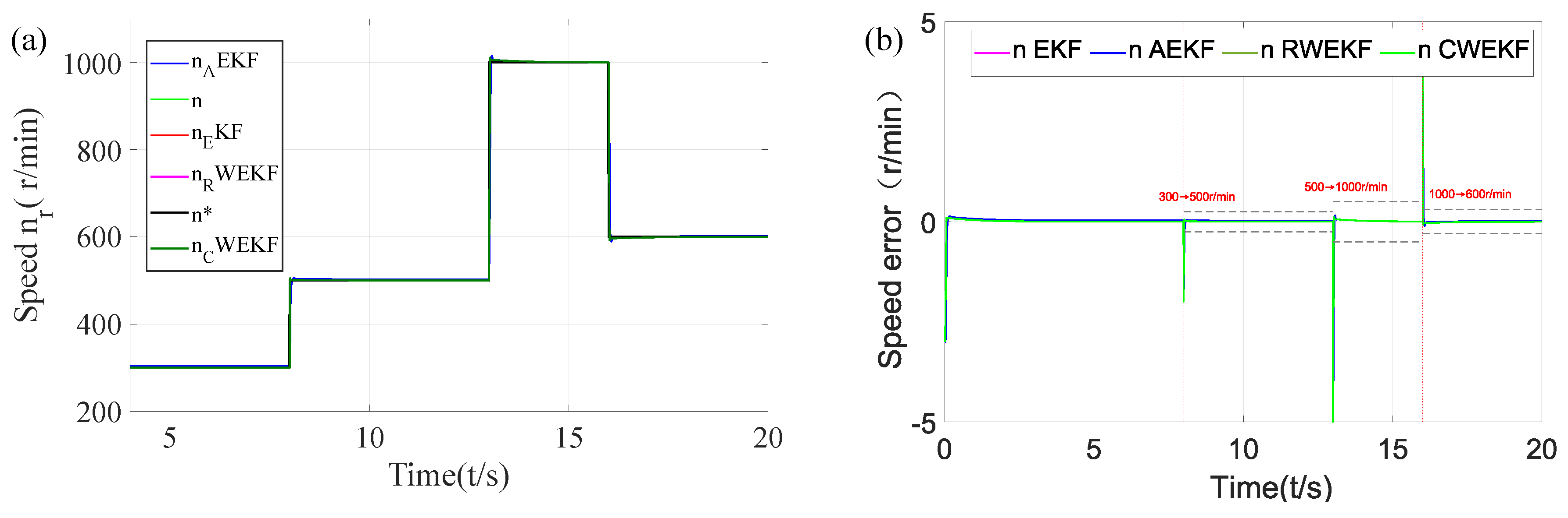
Figure 2.
Rotor flux trajectory estimation of the four algorithms under rotor speed step changes.
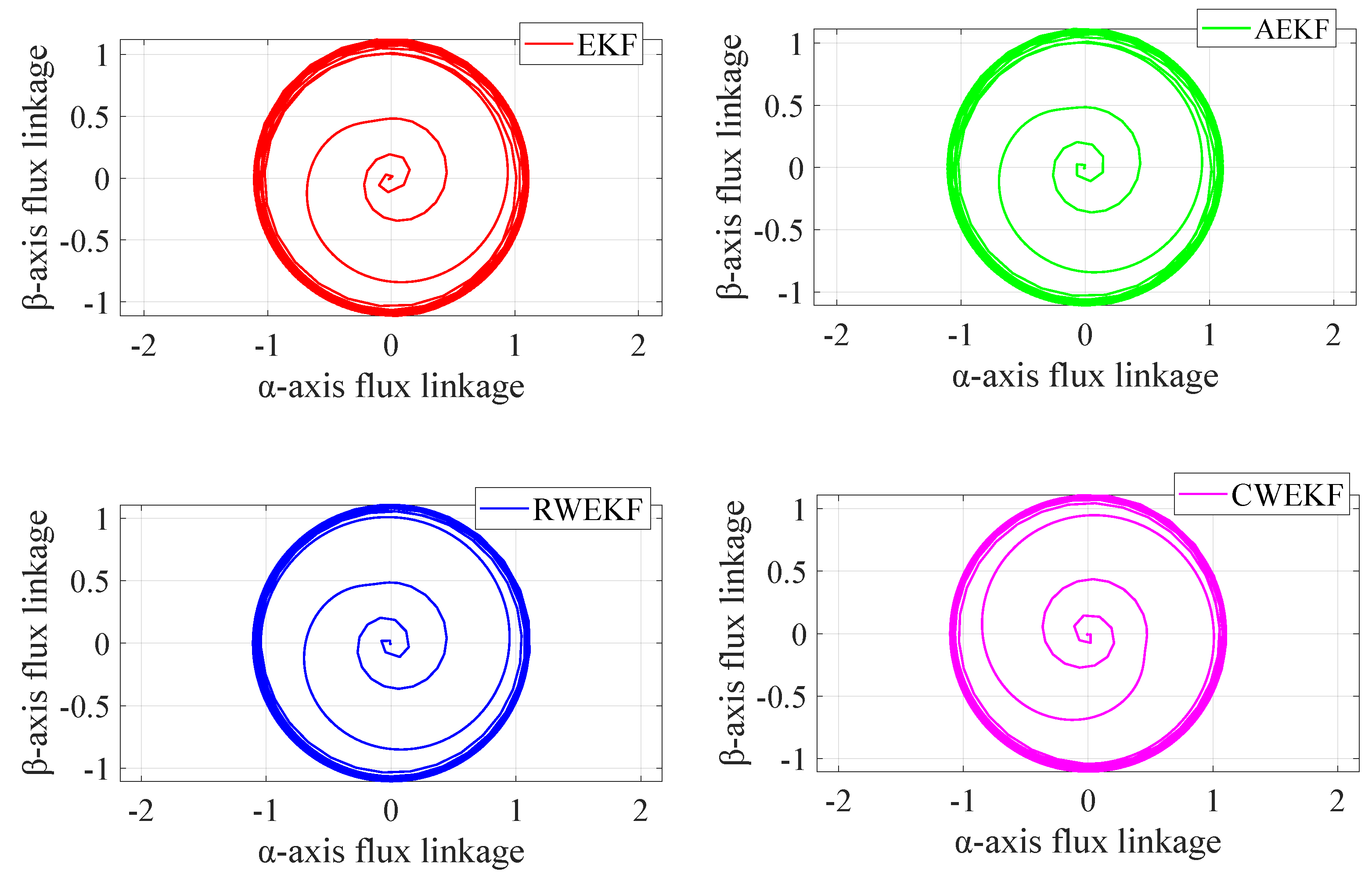
Figure 3.
Rotor current estimation of the four algorithms in the - coordinate system under rotor speed step changes.
Figure 3.
Rotor current estimation of the four algorithms in the - coordinate system under rotor speed step changes.
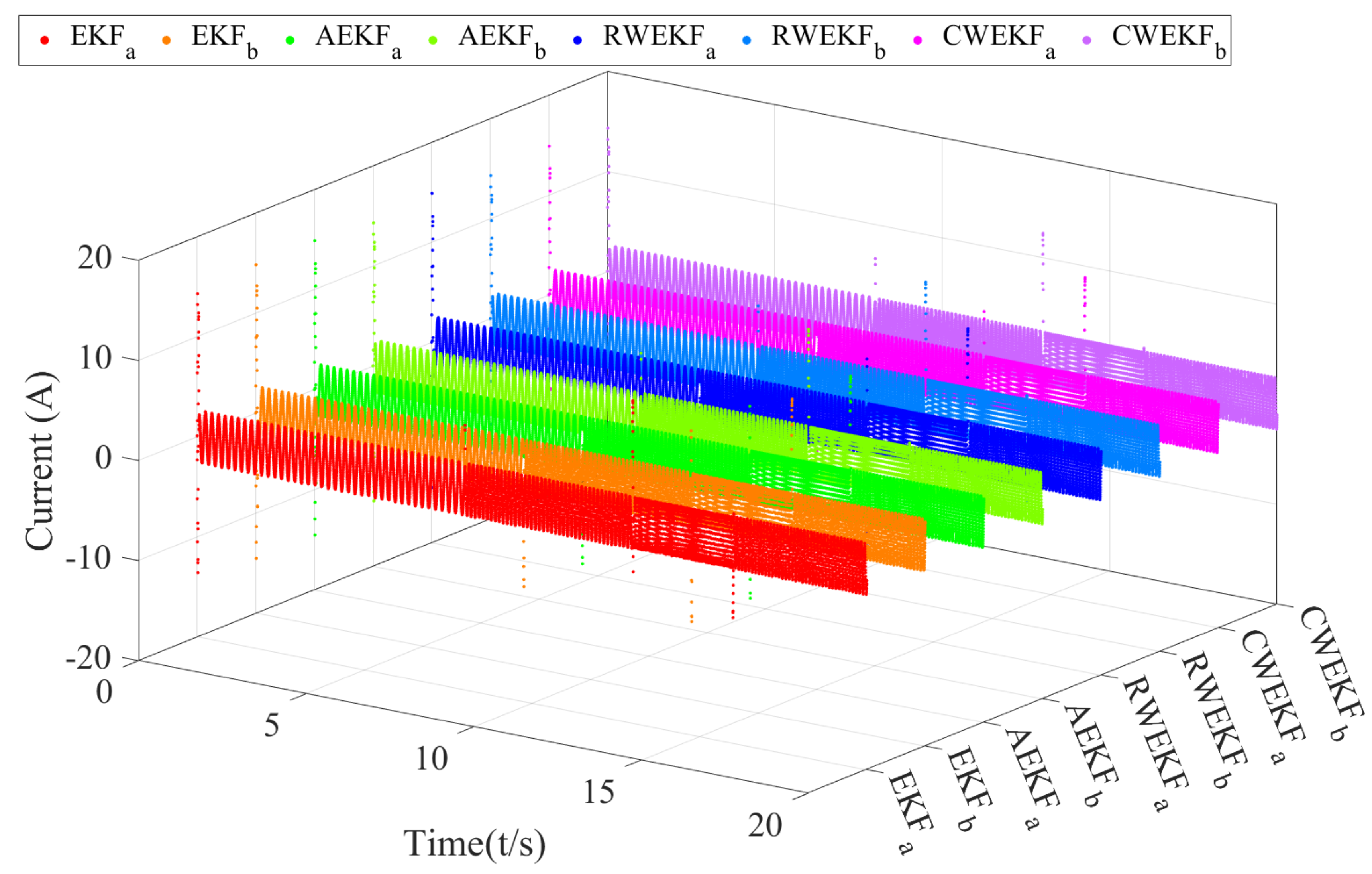
Figure 4.
Changes in values of the four algorithms under sudden speed changes.(a) value of EKF;(b) First 4 values of EKF;(c) value of AEKF;(d) First 4 values of AEKF; (e) value of RWEKF;(f) First 4 values of RWEKF; (g) value of CWEKF; (h) First 4 values of CWEKF
Figure 4.
Changes in values of the four algorithms under sudden speed changes.(a) value of EKF;(b) First 4 values of EKF;(c) value of AEKF;(d) First 4 values of AEKF; (e) value of RWEKF;(f) First 4 values of RWEKF; (g) value of CWEKF; (h) First 4 values of CWEKF
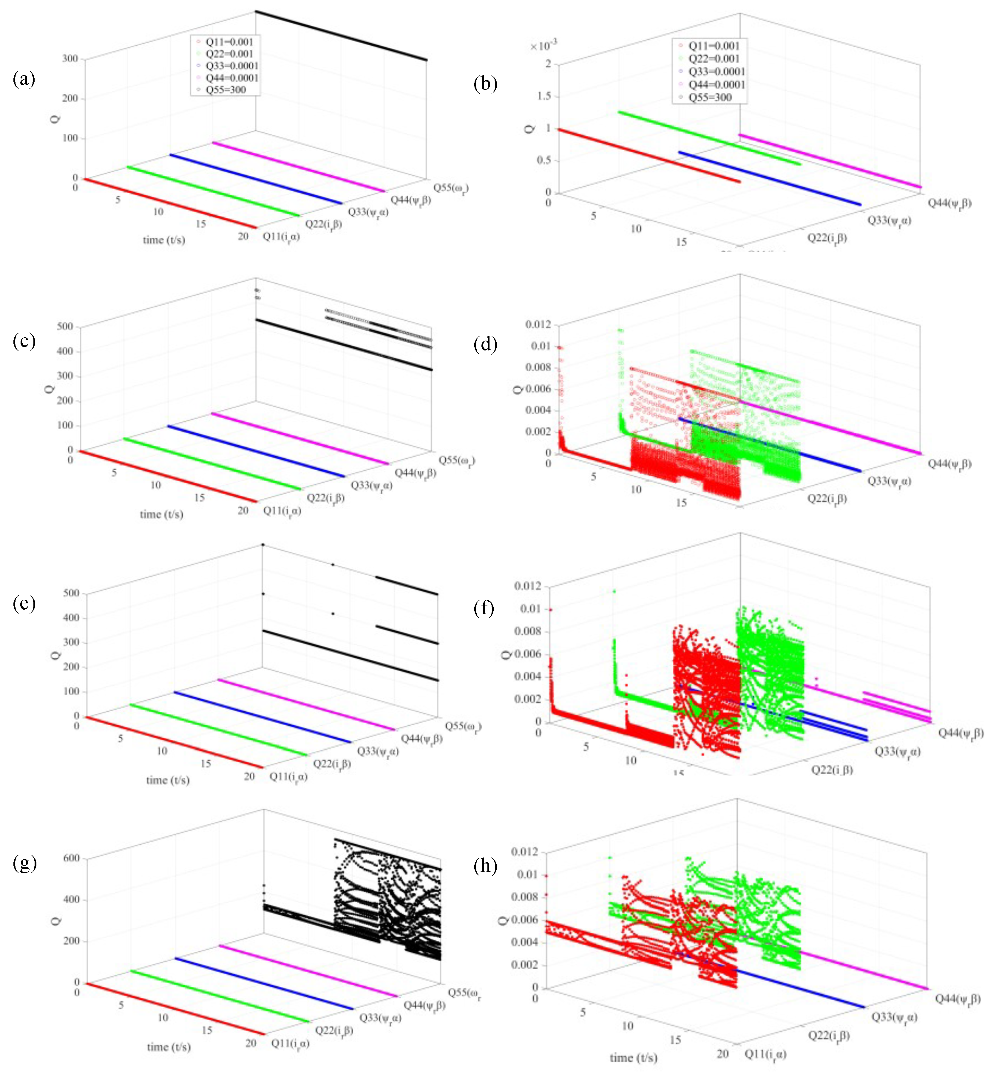
Figure 5.
Changes in values of the four algorithms under sudden speed changes.(a) value variations of EKF; (b) value variations of AEKF; (c) value variations of RWEKF; (d) value variations of CWEKF.
Figure 5.
Changes in values of the four algorithms under sudden speed changes.(a) value variations of EKF; (b) value variations of AEKF; (c) value variations of RWEKF; (d) value variations of CWEKF.
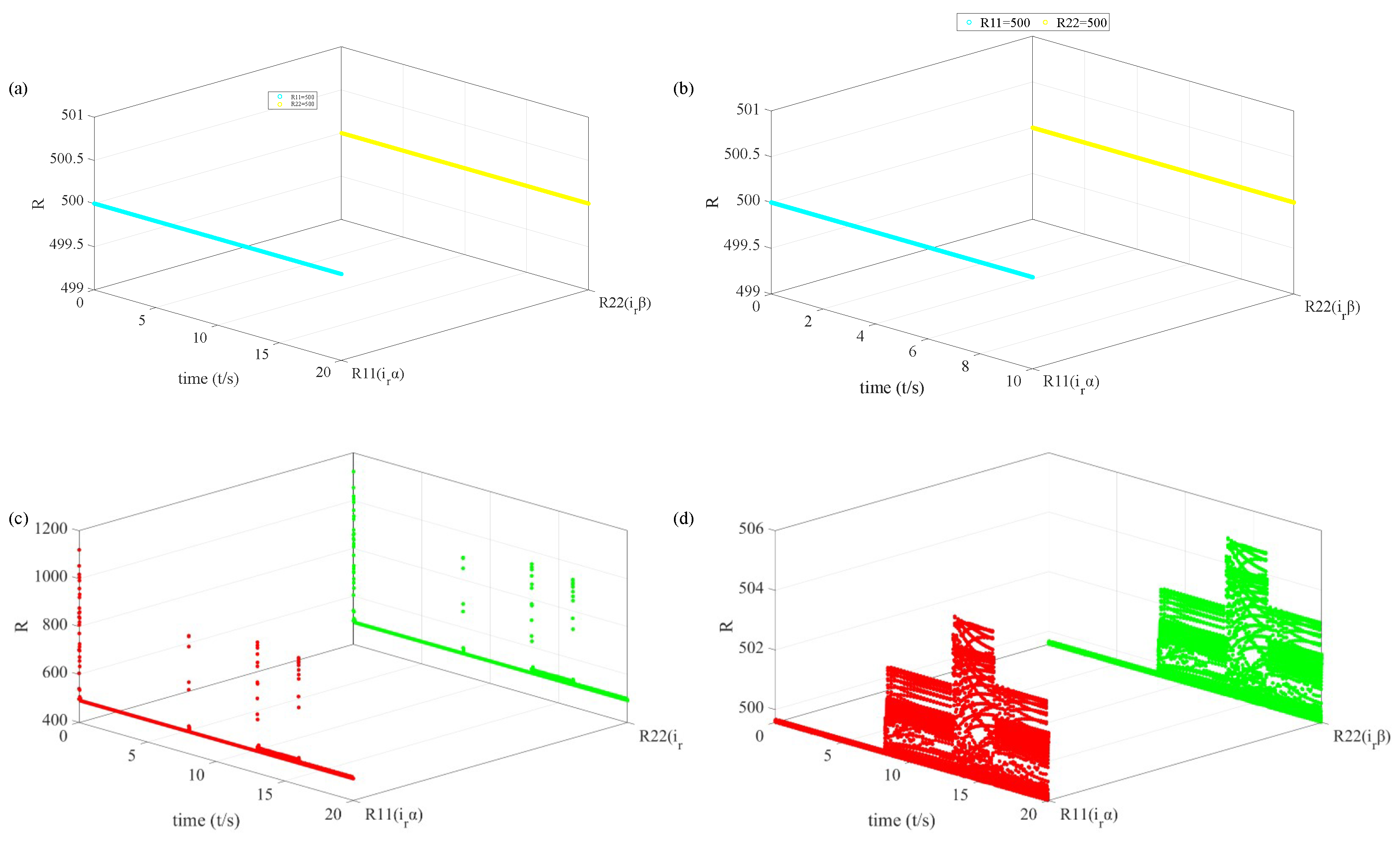
Figure 6.
Comparison of speed estimation and error of the four algorithms under Rs sudden change.
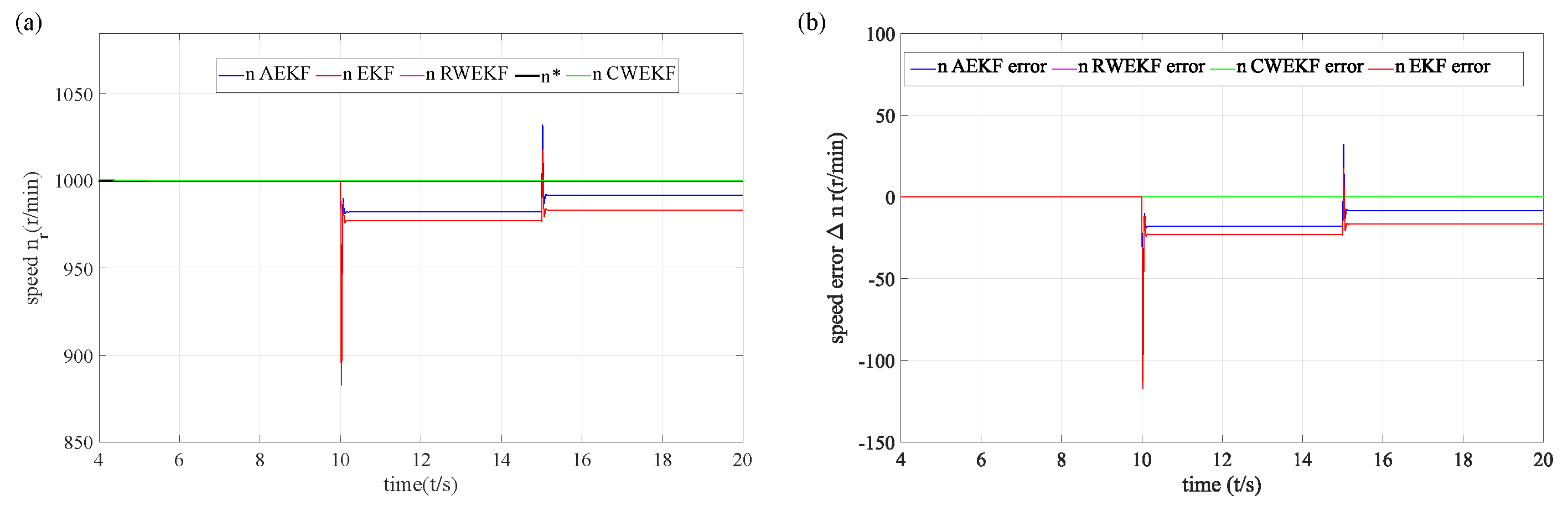
Figure 7.
Rotor flux linkage estimation of the four algorithms under Rs sudden change.
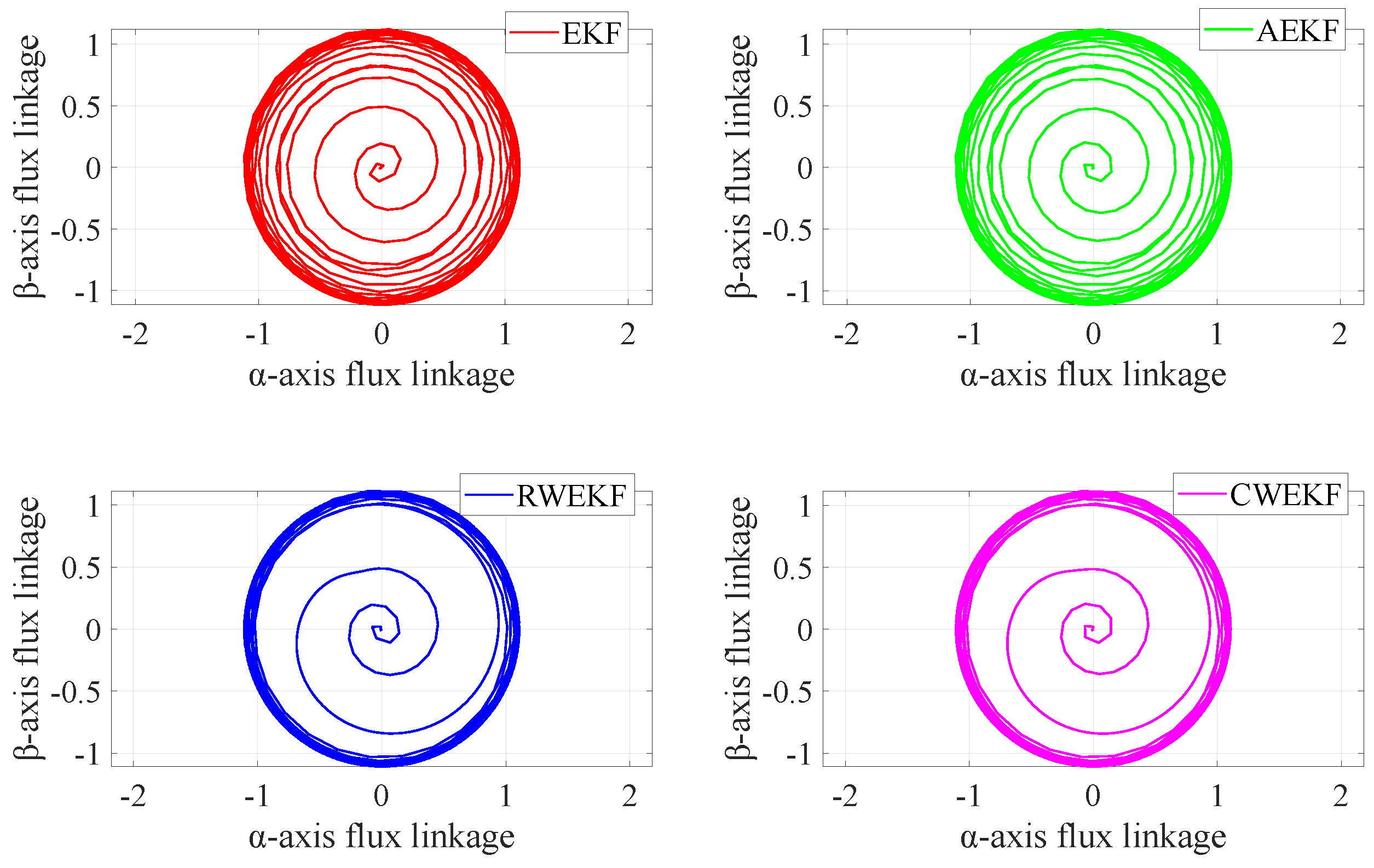
Figure 8.
Rotor current estimation of the four algorithms under Rs sudden change.
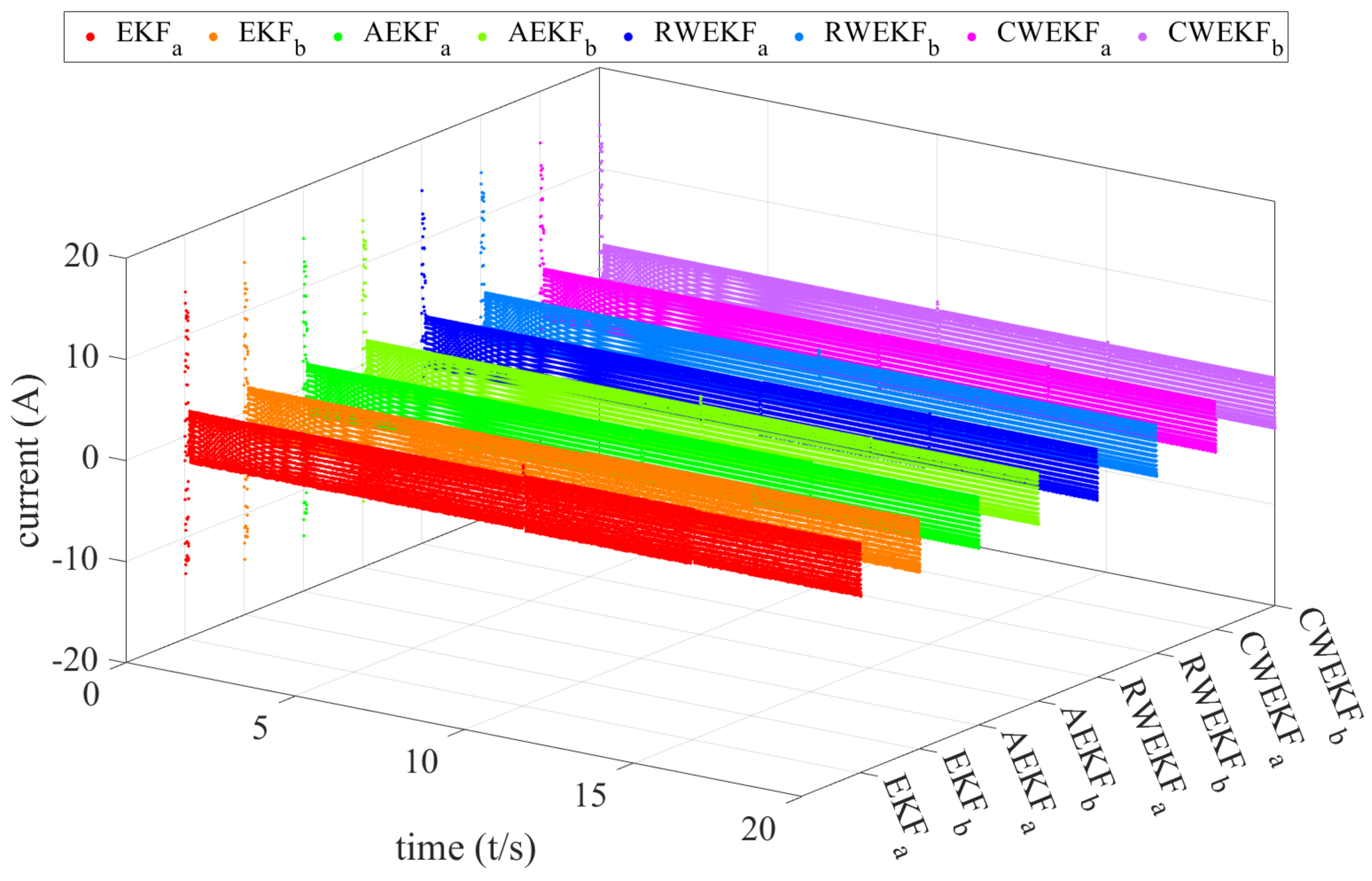
Figure 9.
Changes in values of the four algorithms under Rs sudden change.(a) value of AEKF; (b) The first 4 values of AEKF;(c) value of RWEKF ; (d) The first 4 values of RWEKF; (e) value of CWEKF;(f) The first 4 values of CWEKF.
Figure 9.
Changes in values of the four algorithms under Rs sudden change.(a) value of AEKF; (b) The first 4 values of AEKF;(c) value of RWEKF ; (d) The first 4 values of RWEKF; (e) value of CWEKF;(f) The first 4 values of CWEKF.
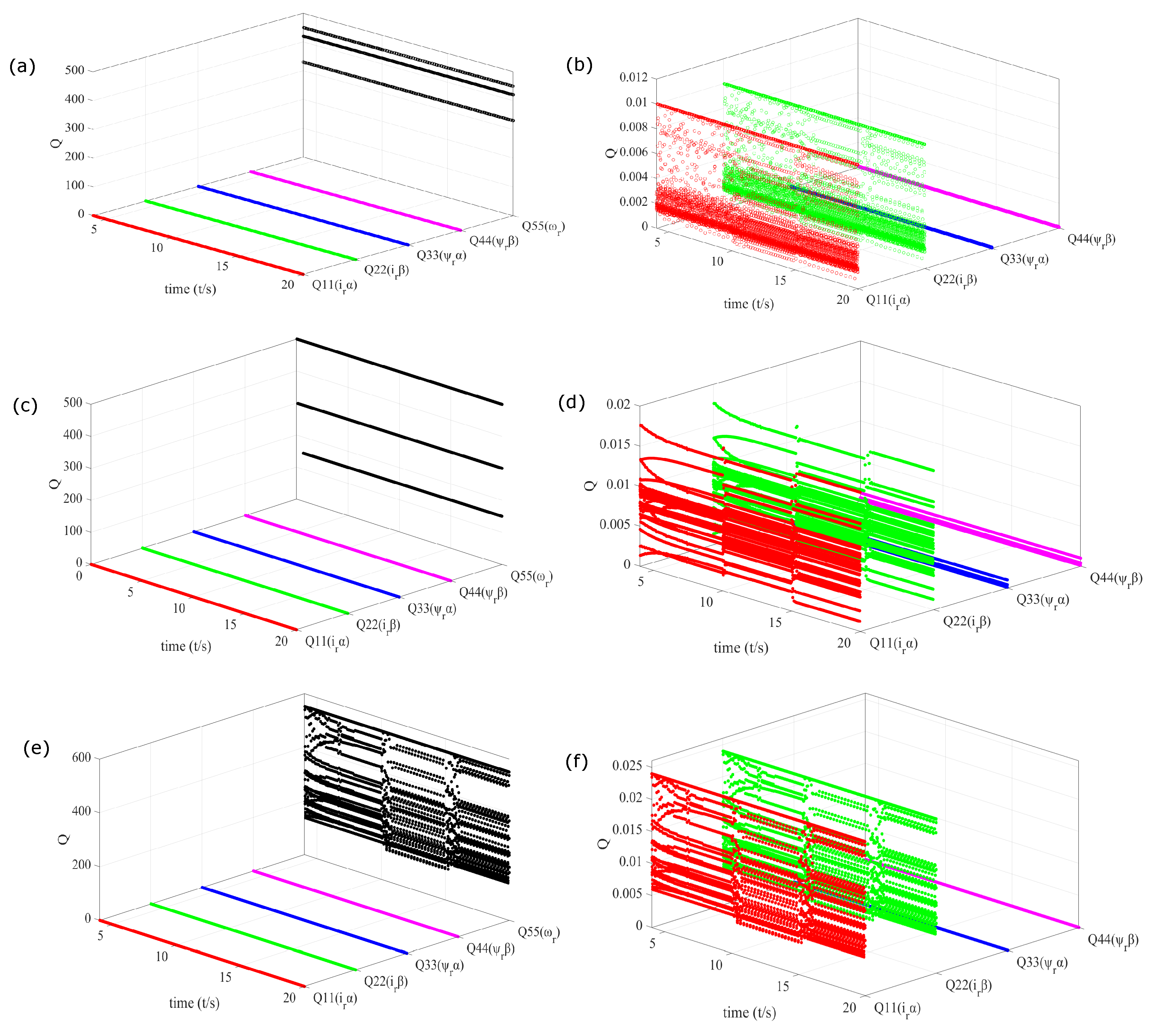
Figure 10.
Changes in values of the four algorithms under Rs sudden change.(a) value variation of RWEKF; (b) value variation of CWEKF
Figure 10.
Changes in values of the four algorithms under Rs sudden change.(a) value variation of RWEKF; (b) value variation of CWEKF
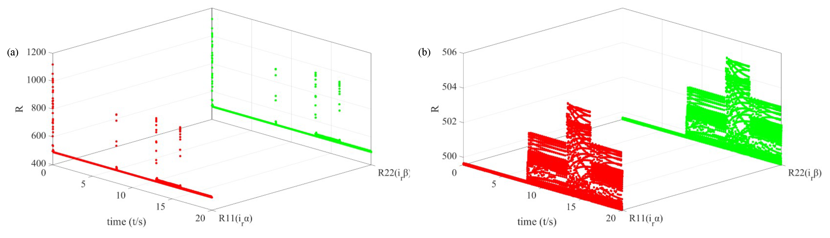
Figure 11.
Speed estimation and error comparison of four algorithms with rotor current noise interference. (a) Speed estimation; (b) Speed error comparison.
Figure 11.
Speed estimation and error comparison of four algorithms with rotor current noise interference. (a) Speed estimation; (b) Speed error comparison.
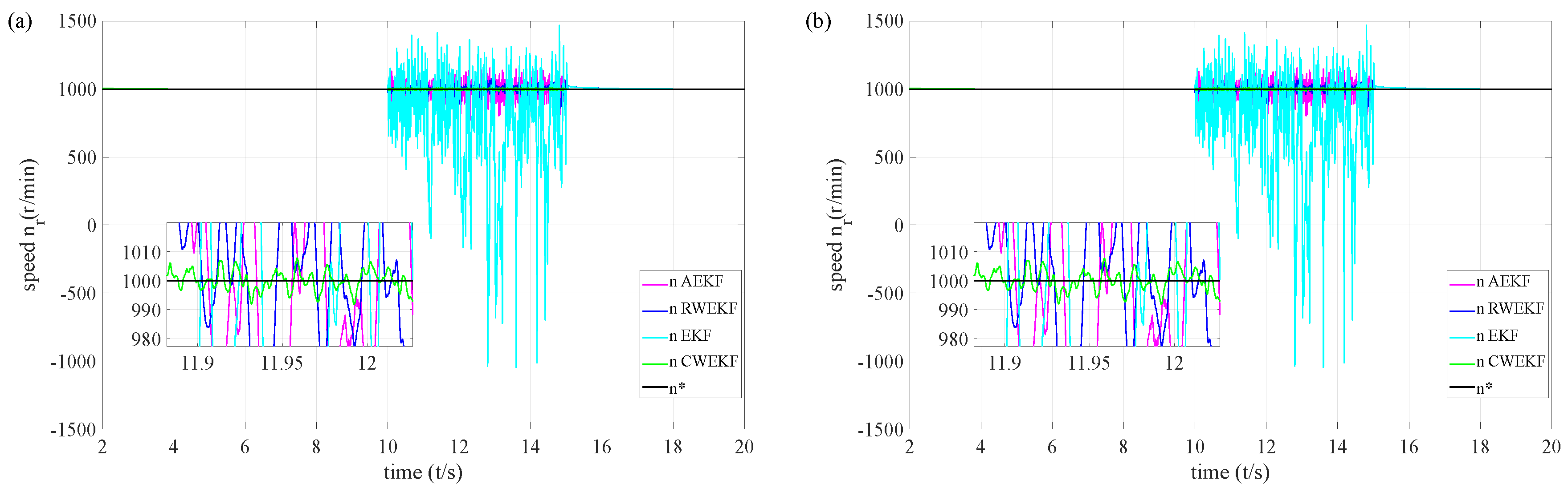
Figure 12.
Flux estimation of four algorithms under rotor current noise interference.
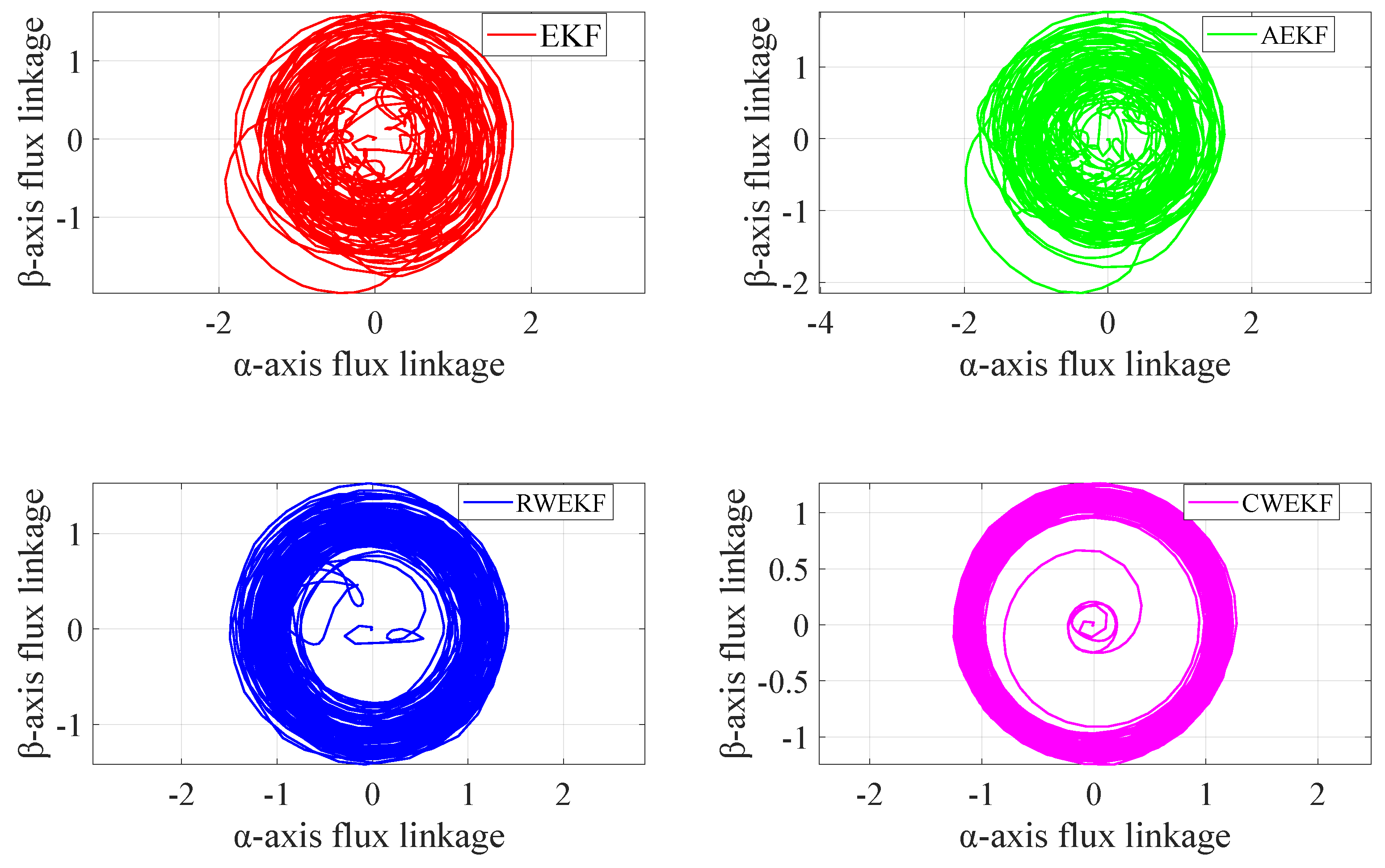
Figure 13.
Rotor current estimation of four algorithms under rotor current noise interference.
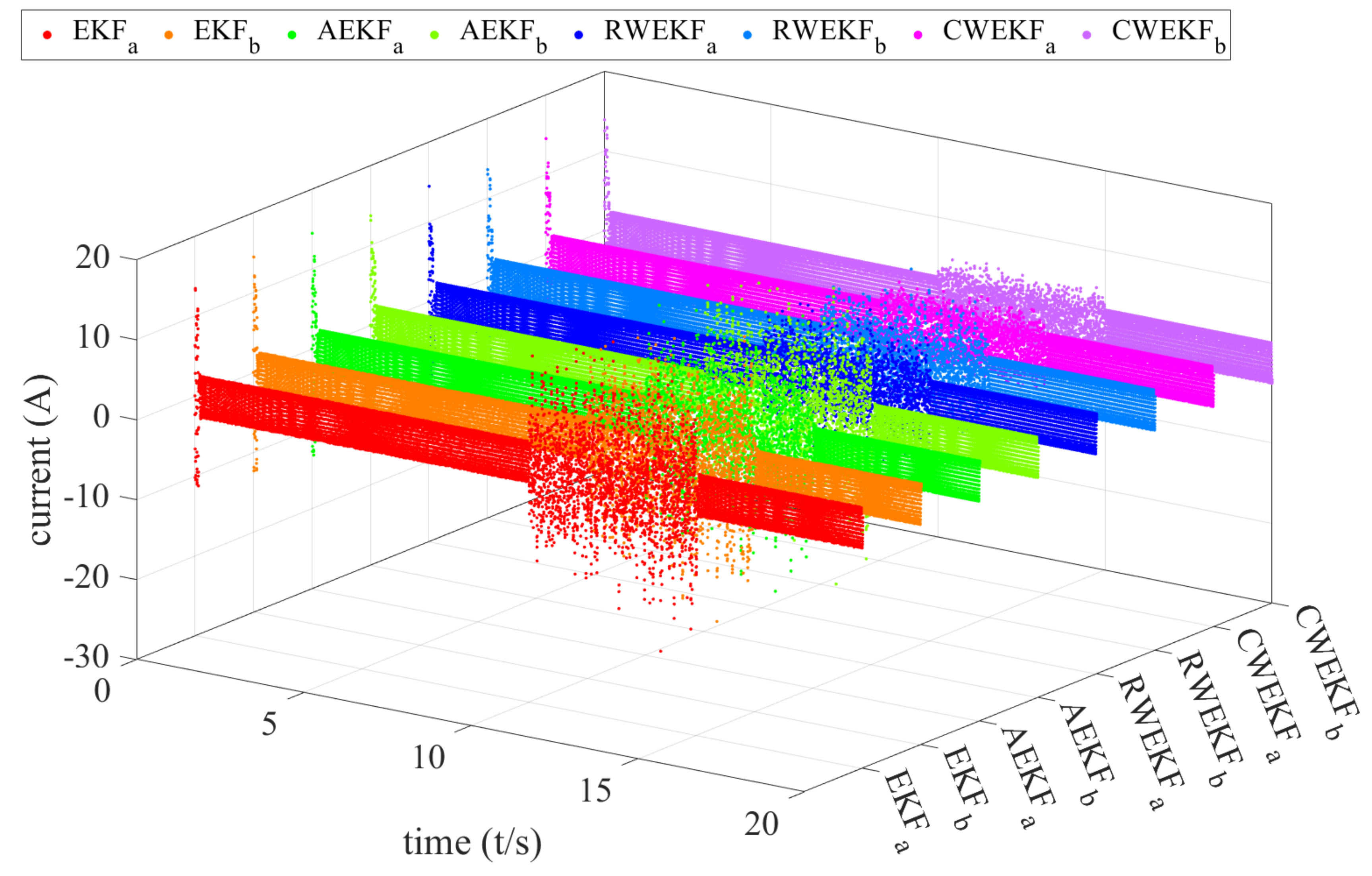
Figure 14.
value variations of four algorithms under rotor current noise interference.(a) value of AEKF; (b) First 4 values of AEKF; (c) value of RWEKF; (d) First 4 values of RWEKF; (e) value of CWEKF; (f) First 4 values of CWEKF.
Figure 14.
value variations of four algorithms under rotor current noise interference.(a) value of AEKF; (b) First 4 values of AEKF; (c) value of RWEKF; (d) First 4 values of RWEKF; (e) value of CWEKF; (f) First 4 values of CWEKF.
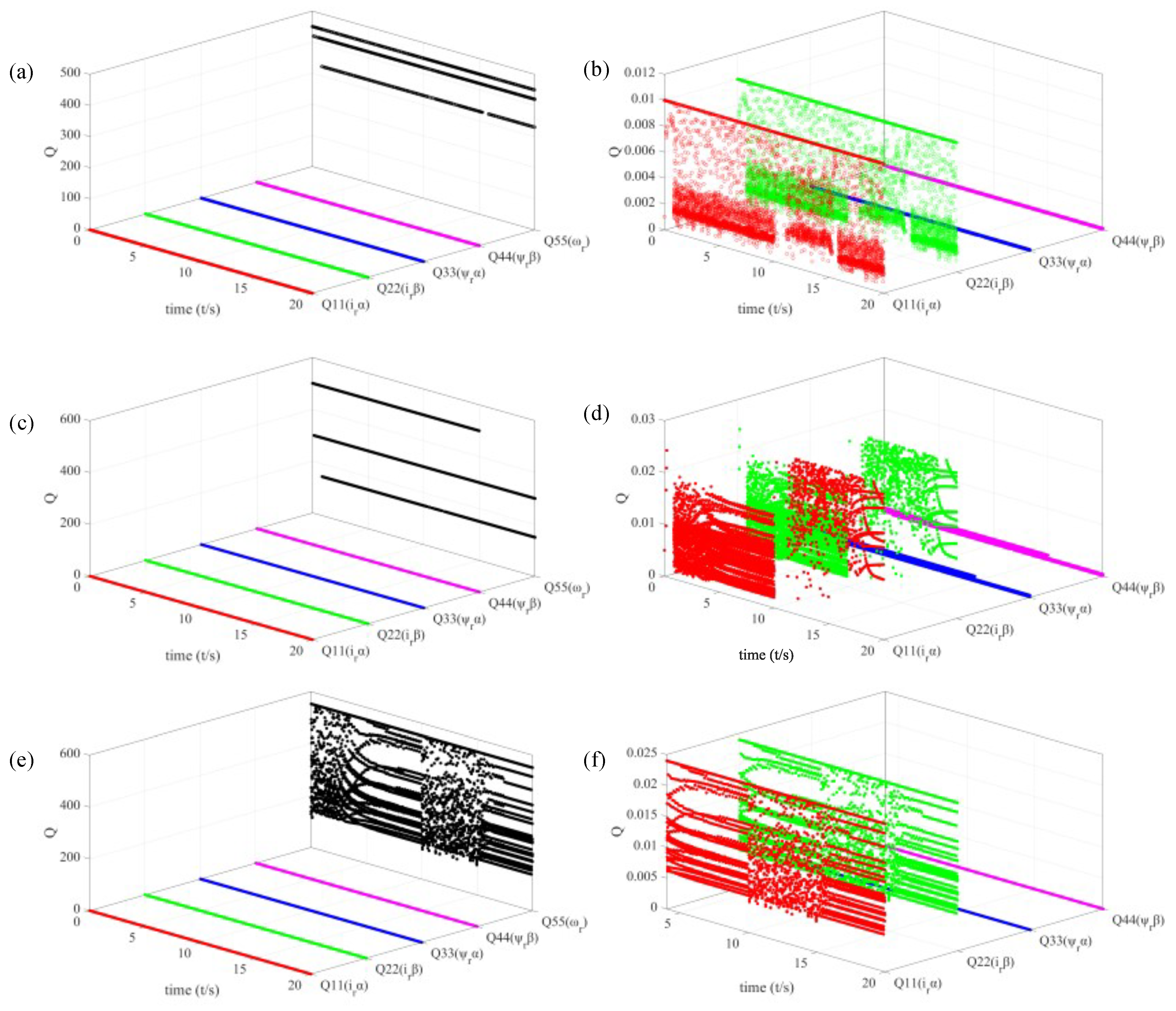
Figure 15.
value variations of four algorithms under rotor current noise interference. (a) value variation of RWEKF; (b) value variation of CWEKF.
Figure 15.
value variations of four algorithms under rotor current noise interference. (a) value variation of RWEKF; (b) value variation of CWEKF.
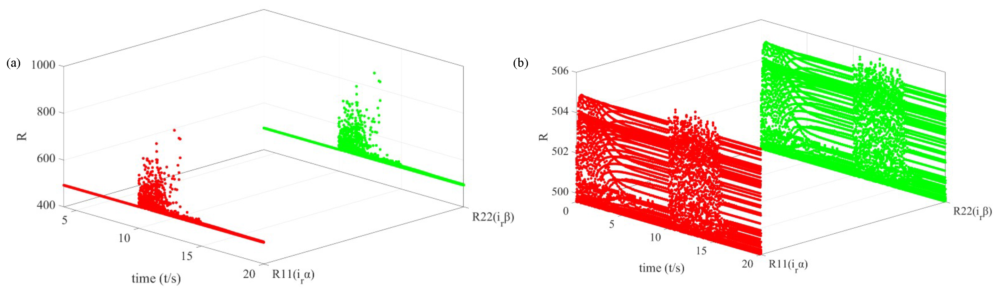

Table 1.
Comparison of overshoot and response time for the four algorithms
| Algorithm | 300–500 r/min | 500–1000 r/min | 1000–600 r/min | |||
| Speed | Overshoot (%) |
Response Time (s) |
Overshoot (%) |
Response Time (s) |
Overshoot (%) |
Response Time (s) |
| EKF | 0.112 | 0.063 | 0.403 | 0.134 | -0.667 | 0.046 |
| AEKF | 0.112 | 0.063 | 0.403 | 0.132 | -0.667 | 0.046 |
| RWEKF | 0.116 | 0.022 | 0.404 | 0.092 | -0.668 | 0.024 |
| CWEKF | 0.116 | 0.022 | 0.404 | 0.092 | -0.668 | 0.023 |
Disclaimer/Publisher’s Note: The statements, opinions and data contained in all publications are solely those of the individual author(s) and contributor(s) and not of MDPI and/or the editor(s). MDPI and/or the editor(s) disclaim responsibility for any injury to people or property resulting from any ideas, methods, instructions or products referred to in the content. |
© 2026 by the authors. Licensee MDPI, Basel, Switzerland. This article is an open access article distributed under the terms and conditions of the Creative Commons Attribution (CC BY) license (http://creativecommons.org/licenses/by/4.0/).
Copyright: This open access article is published under a Creative Commons CC BY 4.0 license, which permit the free download, distribution, and reuse, provided that the author and preprint are cited in any reuse.


