Submitted:
10 February 2026
Posted:
12 February 2026
You are already at the latest version
Abstract
We present a high-fidelity aerodynamic shape optimization framework for the NREL S809 airfoil using Free-Form Deformation (FFD) parameterization coupled with a RANS CFD solver and a discrete adjoint for gradient computation. The design objective is to maximize aerodynamic efficiency (lift-to-drag ratio, CL/CD) under single- and multi-point operating conditions relevant to horizontal-axis wind turbines. Geometry changes are controlled by 40 FFD surface control points, and the Sequential Least Squares Programming (SLSQP) algorithm enforces lift, thickness and volume constraints. We validate our solver against NREL Phase VI wind-tunnel data and perform mesh-convergence and gradient-verification studies. Single-point optimization yields a CL/CD increase of ≈22.5% relative to the baseline at Re = 3.48×10⁶, while multi-point optimizations (2–4 points) produce robust improvements across the operating envelope. We discuss sensitivity to turbulence/transition modeling, show gradient check results (finite-difference vs adjoint), and provide mesh-independence evidence. The optimized shapes reduce maximum thickness and move camber forward, improving lift while reducing drag; however, structural implications of thickness reduction are discussed. The framework and validation illustrate a reproducible path for high-fidelity airfoil optimization targeted at wind-energy applications.
Keywords:
wind turbine
; airfoil
; CFD
; free form deformation
; aerodynamic optimization
1. Introduction
Wind energy has been harnessed for centuries, yet fossil fuels became the dominant source post-industrialization. The International Energy Agency estimates that coal, natural gas, and oil will deplete in 139, 49, and 54 years, respectively[1]. As environmental concerns over fossil fuels grow, transitioning to renewable energy sources like wind, solar, and nuclear is crucial for sustainability. Policy support for reducing greenhouse emissions is boosting wind energy's popularity as shown in Figure 1. In 2022, onshore wind energy costs fell to USD 0.033/kWh, making it much cheaper than fossil fuels, while offshore wind costs slightly increased to USD 0.081/kWh [2]. Advancements in Horizontal Axis Wind Turbines (HAWT) and Vertical Axis Wind Turbines (VAWT) are driving renewable energy progress, with HAWTs enhancing large-scale efficiency and VAWTs improving urban adaptability.
An essential factor in decreasing energy costs in the wind turbine sector is the advancement of airfoils with optimized aerodynamic characteristics. The design of these airfoils is essential for optimizing energy output and overall efficiency, particularly as wind farms mature. Contemporary wind farms exhibit a decline in power generation over time, with capacity factor reductions between 10% and 15% relative to initial manufacturer forecasts [4]. The losses are largely ascribed to airfoil deterioration, heightened surface roughness, and alterations in aerodynamic performance resulting from wear and environmental exposure. Consequently, improving airfoil designs is crucial for sustaining energy output, minimizing operational expenses, and prolonging the lifespan of wind turbines. Optimizing wind turbine blades involves fine-tuning factors like airfoil shape, chord length, thickness, and twist angle distribution [5].
In recent years, the optimization of airfoil shapes has been a central emphasis in enhancing aerodynamic performance, especially regarding renewable energy. Diverse methodologies have been investigated to enhance airfoil designs, encompassing gradient-based methods and sophisticated evolutionary algorithms. For example, the reshaping of airfoils by parameterization approaches like as PARSEC and CST, in conjunction with these algorithms, has produced encouraging outcomes in improving lift and overall aerodynamic efficacy. Notably, a gradient-free method [6] using the Differential Evolution algorithm achieved a 99.8% reduction in drag-to-lift ratio. Additionally, the S809 airfoil was successfully reshaped using PARSEC and a Nash equilibrium genetic algorithm[7], yielding optimal results on the Pareto front. This research [8] series optimized airfoil chord lengths and twist angles using Bezier curves, a MATLAB GA optimizer, and NREL's FAST Framework, significantly enhancing AEP and reducing costs for the NREL 5MW and a custom turbine.Subsequent studies [9] used a GA with CST and PARSEC methods, and XFOIL calculations, to significantly increase lift coefficient and lift-to-drag ratio, enhancing wind turbine blade design. Another study [10] optimized NREL S-821 and RAE-2822 airfoils using CST parametrization and a MATLAB-based GA, alongside the panel method, leading to significant enhancements in lift-to-drag ratios, validated by XFOIL, NREL data, and complemented by CFD analysis. Research [11] utilized CST parametrization with a MATLAB GA, incorporating fitness estimations from Hess-Smith panel method and XFOIL, validated using Ansys-Fluent, to develop an airfoil with superior aerodynamic attributes. In addition of that , this study [12] employs Bézier curves to generate airfoil polar points, utilizes XFOIL as a flow solver, and implements a genetic algorithm in MATLAB for optimization, resulting in a newly optimized airfoil shape that produces greater lift compared to the original design, with additional flow analysis conducted using ANSYS Fluent. Subsequently, a study [13] introduced a machine learning-based algorithm combining CST with XFOIL for improved lift-to-drag ratio optimization, demonstrating superior convergence and performance over conventional GA methods. Furthermore a multifidelity local search algorithm using manifold mapping (MM) efficiently simulated high-fidelity models with low-fidelity ones, drastically reducing computational demands. Tested against transonic flow problems, it performed comparably to the gradient-based SLSQP but proved more cost-effective and scalable, despite a slight increase in drag count [14] . Additionally, a novel approach introduced a deep learning-based surrogate model, combining CST and Latin hypercube sampling, to optimize rotor airfoil aerodynamics and minimize dynamic stall, leading to significant improvements in drag and moment coefficients while enhancing lift [15]. One study[16] applied the CST technique and a modified XFOIL panel code with a derivative-free Covariance Matrix Adaptation Evolution Strategy to design airfoils for megawatt-class wind turbine rotor blades, achieving equal or improved performance compared to Delft University designs. Lastly, the optimization of the NACA 4412 airfoil was conducted using genetic algorithms and particle swarm optimization in MATLAB, with cubic spline, PARSEC, and CST methods for parameterization, while XFOIL served as the flow solver, and CFD simulations using ANSYS FLUENT validated the results, focusing on maximizing lift and minimizing drag [17]. A notable study [18] introduced a fast, interactive design framework for airfoil aerodynamic optimization, employing a B-spline-based generative adversarial network and various neural network models to predict aerodynamic responses, achieving results that closely align with traditional CFD methods while significantly reducing computation time to just seconds .
High-fidelity aerodynamic shape optimization (ASO) models rely on complex, non-linear Partial Differential Equations (PDEs) essential for both 2D and 3D optimizations. One major challenge in this area is the accurate differentiation of these PDEs, which often limits research in gradient-based high-fidelity ASO. Despite their computational demands, high-fidelity models offer highly accurate predictions, making them essential for applications where even small shape changes significantly impact performance, such as in aerospace engineering and airfoil design. Recent advances in ASO research have shifted towards incorporating evolutionary algorithms and machine learning (ML) techniques, diverging from traditional gradient-based methods. For example, one study [19] utilized a multi-objective Genetic Algorithm (MOGA) integrated with FLUENT software’s Reynolds-Averaged Navier-Stokes (RANS) equations for airfoil optimization, which resulted in notable improvements in both lift and lift-to-drag ratios. Another study [20] employed a continuous adjoint method coupled with CFD to explore the influence of turbulence models on NACA 0012 and DU 93-W-210 airfoil shapes. This study successfully optimized the airfoils by increasing lift coefficients by 20% and reducing drag by 3%, achieved through the use of spline control points.
Furthermore, morphing trailing edge optimization using free-form deformation parameterization was examined in [21] , revealing that an optimal number of control points is crucial for avoiding wavy deformations and enhancing optimization accuracy. In my research, I solve RANS equations with a Spalart-Allmaras turbulence model, applying a gradient-based optimization algorithm and adjoint method to calculate necessary derivatives. Similar to previous research [22], this approach achieved an 8.5% reduction in drag through single-point optimization, while considering lift, pitching moment, and geometric constraints. Moreover, multi-point optimization was used to ensure realistic designs, resulting in drag values within 0.1 counts of each other across various conditions.
Additionally, another pivotal study [23] focused on transonic aerodynamic shape optimization of the Common Research Model (CRM) wing benchmark, addressing both computational intensity and design sensitivity. This research employed six benchmark optimizations, ranging from single to nine-point cases with 768 variables, ultimately achieving a 7.5% drag reduction for single-point designs and enhanced robustness for off-design conditions in the nine-point cases. Finally, recent work [24] developed an efficient discrete adjoint framework for shape optimization using OpenFOAM, effectively applying this method to UAV and car designs, reducing drag by 5.6% and 12.1%, respectively.
This research employs an innovative methodology that integrates Free-Form Deformation (FFD) with computational fluid dynamics (CFD) and the adjoint technique, employing the numerical flow field solver and SLSQP optimizer for the optimization of airfoil shapes. The principal benefit of this technique is its capacity to effectively investigate the design space while maintaining high accuracy in aerodynamic forecasts. In contrast to earlier techniques that frequently depend on surrogate models or evolutionary algorithms, our methodology enables direct gradient-based optimization, markedly improving convergence rates and the accuracy of optimum designs. Furthermore, utilizing the adjoint technique enables the rapid computing of sensitivities concerning various design factors, effectively mitigating the scalability and accuracy deficiencies commonly found in conventional optimization frameworks. This feature facilitates a more comprehensive investigation of the parameter space, resulting in enhanced aerodynamic performance and enabling the design of airfoils that satisfy the requirements of contemporary renewable energy applications. Collectively, these research exemplify the incremental amalgamation of evolutionary algorithms, machine learning, and computational fluid dynamics in enhancing aerodynamic optimization, indicating the possibility for substantial advancements in airfoil design efficacy.
This study is organized as follows. Section 2 describes the methodology for airfoil shape optimization, including the use of Free-Form Deformation (FFD) for parameterization, mesh generation and deformation processes, the CFD solver, the discrete adjoint method, and the SLSQP optimization algorithm. Section 3 presents and discusses the results of the numerical flow field CFD solver validation, as well as the findings from both single-point and multi-point optimization. Finally, the conclusion summarizes the key insights of the study.
2. Methodology
This section provides a brief summary of the components within the optimization framework, as illustrated in Figure 2 using an extended design structure matrix (XDSM) diagram[25]. The study employs a sophisticated framework designed for high-fidelity aerodynamics and structural optimization, utilizing a direct design approach to iteratively refine airfoil shapes, as depicted in the workflow represented by the XDSM diagram.
The optimization process initiates with the assignment of initial design variable values, x(0), to the optimizer ,which then updates the surface mesh using the surface deformation module in every iteration except the first iteration and computes its analytical derivatives in relation to the design variables expressed as dxs/dx ,followed by volume deformation module modifying the volume mesh and determining its derivatives in relation to the surface mesh changes, notated as dxv/dx , while the flow solver processes flow states denoted as wrelayed to the adjoint solver to calculate the total derivative, culminating in the determination of the objective function f and its derivatives df/dx by the optimizer, with surface and volume deformation steps being quick and explicit and flow and adjoint solver steps being iterative and time-consuming , typically involving about o(102) major iterations, setting a fundamental minimum for the count of CFD solutions and mesh updates required, with each major iteration including additional CFD solutions.
2.1. Geometry Parameterization
The geometry of wind turbine airfoils plays a critical role in the overall performance and efficiency of rotor systems. Among various airfoil designs, the S809 airfoil stands out as a key contributor to advancements in wind turbine technology, particularly within the framework of NREL Phase VI Rotor. This airfoil is specifically engineered to optimize laminar flow, achieving a thickness of 21%, which significantly enhances aerodynamic efficiency.
As illustrated in Table 1 and depicted in Figure 3, the S809 airfoil features a carefully designed tapered and twisted geometry, which is instrumental in maximizing the effectiveness of the rotor's two-bladed configuration [26,27]. Its design principles have been applied consistently in NREL's Phase II, III, and VI (HAWTs), demonstrating its pivotal role in enhancing blade performance throughout their operational length [28]. In light of these attributes, this subsection delves into the geometric parameterization of the S809 airfoil, examining its implications for rotor design and performance optimization in contemporary wind energy systems.
In shape optimization, particularly for airfoil design, geometry parametrization is essential and challenging. The free form deformation (FFD) technique, introduced by Sederberg and Perry [30], is employed to translate design variables into actual geometric changes. It involves applying a grid structure over the object, where modifications to the grid's control points result in the object's indirect deformation as shown in Figure 4. (a) which will be our work on this paper. The FFD volume captures alterations in geometry instead of the geometry itself, leading to a streamlined and concise collection of design variables for the geometry, simplifying the manipulation of intricate shapes.It is straightforward, concise, and effective, with readily calculable analytical sensitivity derivatives suitable for gradient-based optimization techniques.
The subsequent step integrates the method to generate geometry parametrization, constraints, and utility functions for geometry manipulation, particularly notable for its capacity to compute derivatives for all parametrization methods and constraints, as depicted in Figure 4.(b) , where the airfoil section is molded by adjusting 20 FFD control points, distributed evenly between the upper and lower surfaces, thereby yielding 40 variables for shaping the airfoil
2.2. Mesh Generation and Deformation
Before proceeding with the optimization process, mesh generation and deformation are key components in modern CFD applications. It is essential to generate the volume mesh for the baseline S809 airfoil which involves growing or extruding the mesh in successive layers from an initial surface or curve until it extends sufficiently away from the original surface, resulting in the meshing of the entire space surrounding the geometry, as shown in Figure 5.
As shown in Figure 5.b, the O-grid hyperbolic structured mesh generator [31] has superior resilience and convergence speed compared to C-grids. These meshes exhibit exceptional accuracy near edges and demonstrate efficacy under stress situations, provided the spacing is constant. Although there are concerns with element orthogonality in wake regions and numerical instabilities at narrow trailing edges, these problems may often be mitigated by using blunter or rounder trailing edges. The generator demonstrates excellent performance due to its rapid operation and dependability, especially while navigating strongly convex bends.
Throughout the optimization iteration, following the determination of a new airfoil shape using FFD variables, I deform the surface mesh and extend it to the entire volume mesh using an unstructured deformation algorithm, which employs a hybrid method combining algebraic and linear elasticity approaches [32], effectively handling both large-scale and small-scale perturbations in the geometry during the optimization process, while an alternative approach utilizes the inverse distance weighting function (IDW)[33], as demonstrated in Figure 6, showcasing the comparison between the original and deformed mesh of the NREL Phase VI S809 airfoil.
2.3. The High-Fidelity CFD Solver
The high-fidelity CFD solver which has been used in my study, is designed for aerodynamics and multidisciplinary optimization (MDO). It specializes in parallel computing and efficiently processes various equations, including Euler, laminar Navier-Stokes, and Reynolds-averaged Navier-Stokes (RANS), for different simulation types. Utilizing a structured finite volume method, the solver is compatible with structured multiblock meshes and employs the Spalart-Allmaras turbulence model alongside the Jameson–Schmidt–Turkel (JST) scheme for its computations.
The four terms represent the convective, production ,diffusion, and near-wall destruction for the turbulent flow, respectively. where is related to the turbulent viscosity via
Where is the is the modified turbulent viscosity,velocity component ,is the magnitude of the vorticity, is the molecular kinematic viscosity, is the distance to the nearest wall ,,, and are model constants. and empirical damping functions within the model.
The high-fidelity solver employs several numerical schemes for flux calculations and solves compressible flow equations using different turbulence models. It utilizes algorithms such as Runge-Kutta, D3ADI, ANK, and NK to ensure efficient residual convergence. The algorithm specifically designed for overset meshes is particularly effective, while another ensures efficient convergence across all mesh types. Various integration schemes, such as explicit Runge-Kutta, implicit LU-SGS, and DDADI methods, are used depending on the simulation requirements. For turbulence ulfilng, a segregated DDADI scheme is employed to manage factorization errors, enabling accurate and efficient solutions.
2.4. High-Fidelity Gradient-Based with Discrete Adjoint Method
In aerodynamic shape optimization, the adjoint method is efficient in managing multiple design variables, in contrast to traditional finite-difference methods, due to its scalability and reduced computational load. The optimization function (f) relies on design variables (x) that shape the airfoil and flow state variables (w), determined by CFD solvers through residuals R(x,w(x))=0. This function is directly influenced by design variables and indirectly affected by changes in state variables needed to ulfil governing equations. Calculating gradients crucial for gradient-based optimization requires accounting for both dependencies, employing the chain rule for total derivative computation.
Here, explicit function derivatives represent partial derivatives, which can be computed analytically at a low computational cost, whereas obtaining the total derivative necessitates iterative solution of the governing equations; ensuring that the total derivative of the CFD residuals R(x,w(x))=0 with respect to x remains zero for a feasible solution allows determination of the complete derivative of the flow solution regarding design variables dw/dx, with the equations being nonlinear and involving millions of state variables, thus necessitating specialized iterative solvers.
The equation provided facilitates the formulation of a linear system, the solution of which yields the total derivative of the flow solution with respect to the design variables.
I Substituting the Jacobian's solution from the given equation into the total derivative equation Equations (2.3) yields the following result:
The equation solely comprises partial derivative components, computable analytically with minimal computational expense, and the resolution of the linear system can be accomplished either by computing the solution Jacobian dw/dx from Equations (2.4) or by addressing the adjoint system.
The adjoint vector derived from Equation (2.7) can be applied in the total derivative equation, Equation (2.3). This method proves computationally efficient, particularly in 3D aerodynamic shape optimization (ASO), where typically there are fewer than 10 functions of interest, compared to potentially hundreds of design variables.
In summary, a discrete adjoint involves four main steps:
- 1)
- Compute and
- 2)
- Solve the adjoint equation to obtain
- 3)
- Compute and
- 4)
- Compute the total derivative .
In summey for above mentioned here summeries in this Figure 7 that show optimization loop using the SLSQP optimizer flowchart , where design variables x are used to update the geometry and mesh, feeding into the flow solver that solves the RANS equation R(x,w(x))=0 to determine state variables w. The adjoint solver then computes the total derivative df/dx using the equations and , which are fed back into the optimizer to refine the design variables.
2.5. Optimization Algorithm
In this research, I utilize the Sequential Least Squares Programming (SLSQP) algorithm [34] for all optimization tasks. This algorithm is specifically designed to address nonlinear optimization problems with both equality and inequality constraints, aiming to identify the minimum or maximum of a function subject to these constraints. It achieves this by approximating the objective function and constraints, integrating methods from least squares and quadratic programming. The SLSQP algorithm iteratively refines the solution using the Han-Powell quasi-Newton method, updating the B-matrix according to the BFGS formula and incorporating an L1-test function within its step-length algorithm, which is associated with the reciprocal of the Hessian matrix. The stopping criterion for this algorithm is based solely on the objective function, terminating when the absolute difference between the objective function value at the current iteration (M(k)) and the previous iteration (M(k-1)) is less than the product of a predetermined tolerance (eM) and the current value. For the purposes of our research, this tolerance has been set to 10-7.
3. Results
3.1. Flow Field Numerical Simulation Validation
The validation of flow field numerical simulation is conducted through a rigorous comparative analysis of its results against empirical data and established computational fluid dynamics (CFD) methodologies. This validation process is essential for ensuring the accuracy and reliability of aerodynamic simulations. The study utilizes an O-type computational domain, with the mesh settings specifying an outer sub-domain radius of 20c, as illustrated in Figure 7. The initial mesh point is positioned at 1.236 × 10⁻⁵ meters from the airfoil, achieving a y+ value of less than 1, which results in a total mesh comprising approximately 67,304 cells. The flow field analysis is performed on the S809 airfoil across angles of attack (AOA) ranging from 0° to 16° at a Reynolds number of 2 × 10⁶.
As depicted in Figure 9.a, the numerical flow simulation demonstrates comparable lift coefficient results that closely align with experimental data up to an AOA of 9 degrees. Beyond this point, the experimental data exhibits a divergence, indicating flow separation that is not accurately captured by the simulations. Figure 9.b illustrates the corresponding trends in drag coefficients, where both solvers exhibit agreement until 9 degrees AOA. Subsequently, the numerical flow simulation indicates a marked increase in drag relative to the experimental observations, suggesting potential overestimation of drag or inadequacies in capturing post-stall flow dynamics.
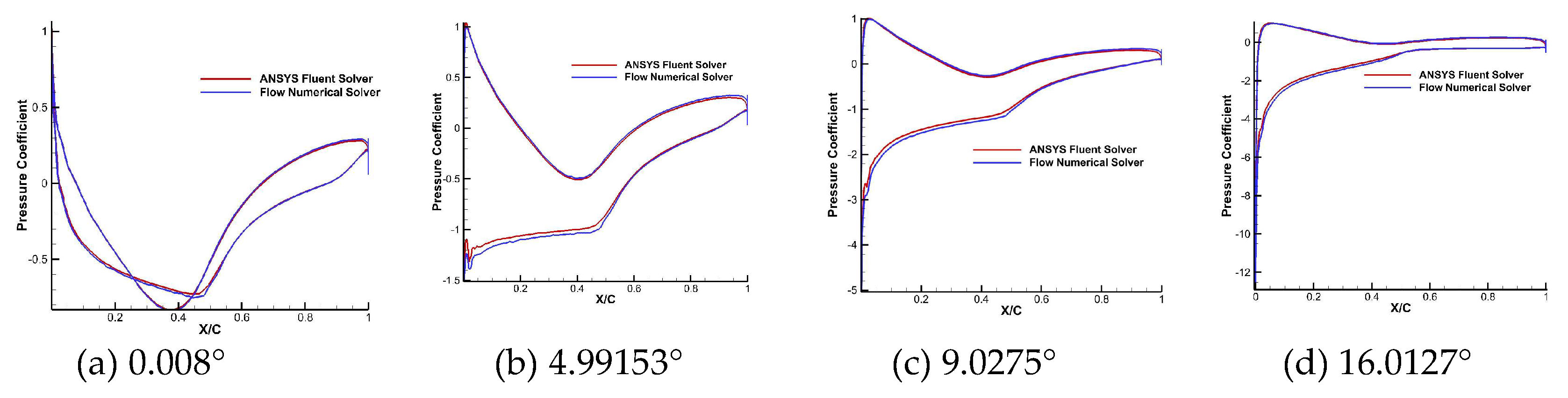
Both solvers employ numerical simulations to solve the Navier-Stokes equations and the energy equation, utilizing the Spalart-Allmaras turbulence model to predict airflow behavior around the S809 airfoil. The numerical results are validated by comparing the outputs from both solvers against experimental data. Figure 9 through 12 provide visual representations of pressure and velocity contours, streamlines, and pressure variations on the airfoil surface at attack angles of 0.008°, 4.99153°, 9.0275°, and 16.0127°. The comparative analysis indicates that both numerical flow simulations yield closely aligned predictions across the examined angles, thereby corroborating the efficacy of the numerical methods as reliable tools for aerodynamic simulations.
Figure 8.
Structured O-Grid for NREL S809 Airfoil.
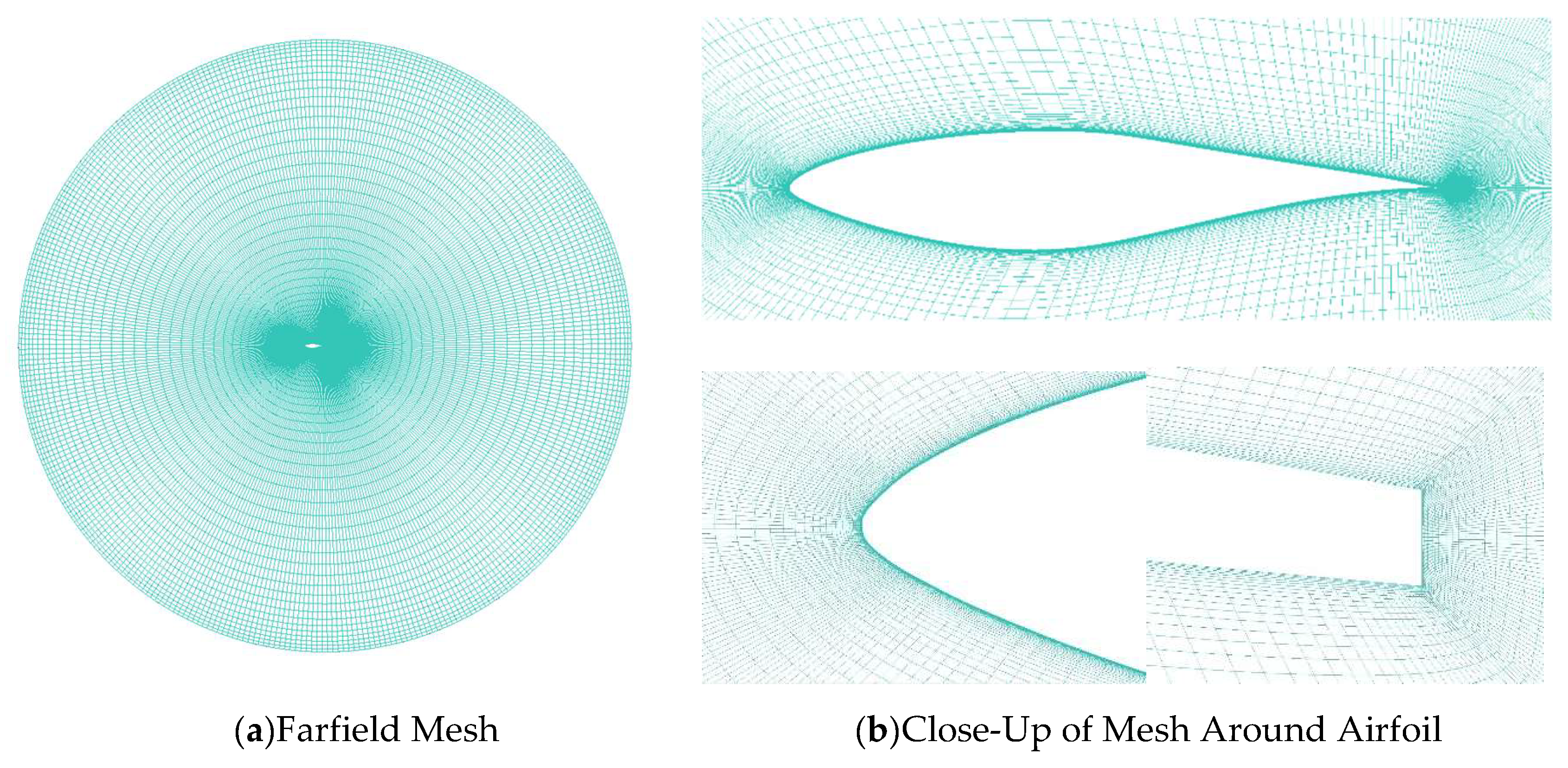
Figure 9.
Comparative Analysis of S809 Airfoil Using Fluent and Flow Numerical Solvers at Re=2e6 with Experiment Data.
Figure 9.
Comparative Analysis of S809 Airfoil Using Fluent and Flow Numerical Solvers at Re=2e6 with Experiment Data.
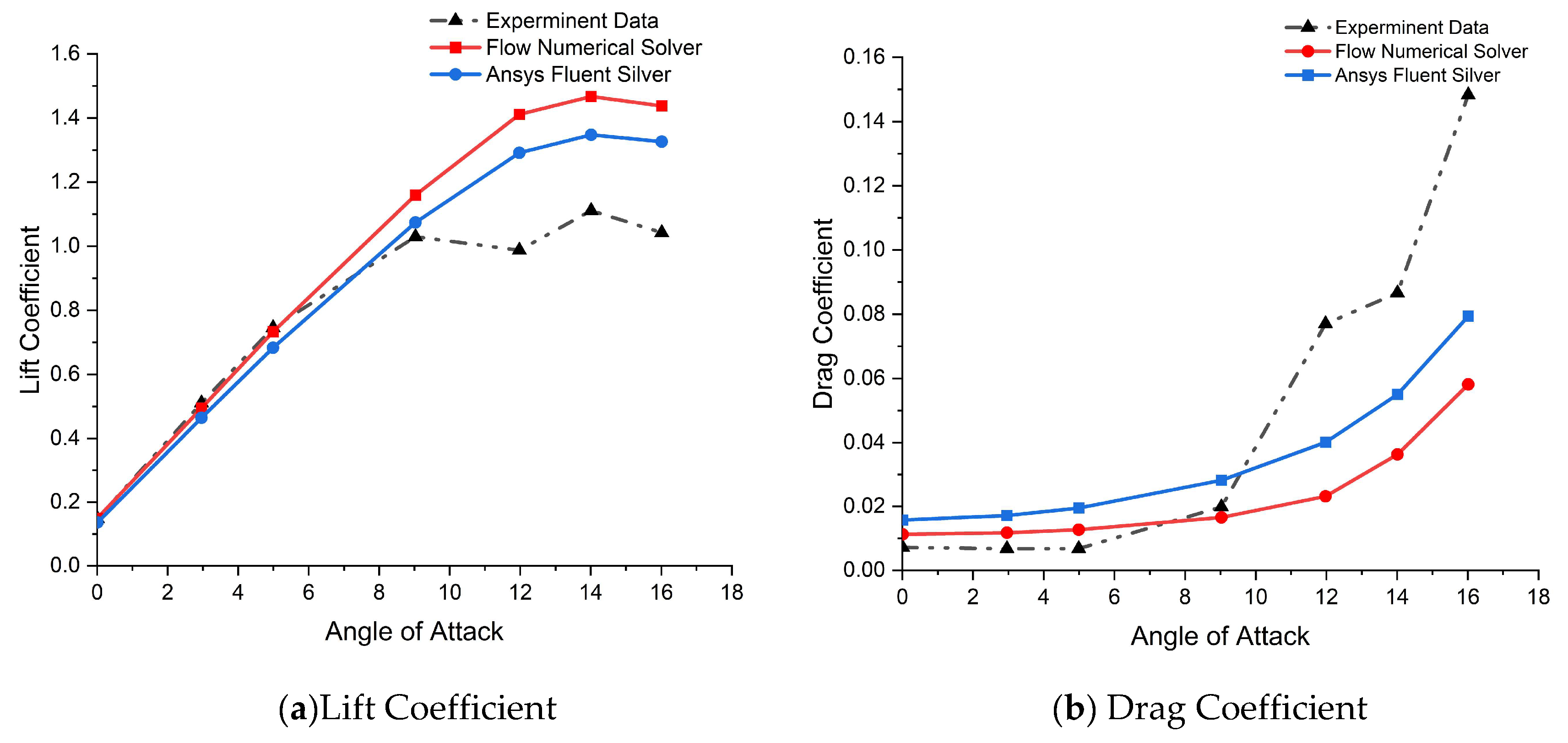
Figure 10.
The Pressure Contour at Different Angle of Attack by (a-d) Flow Numerical Solver,(e-h) Fluent Solver.
Figure 10.
The Pressure Contour at Different Angle of Attack by (a-d) Flow Numerical Solver,(e-h) Fluent Solver.
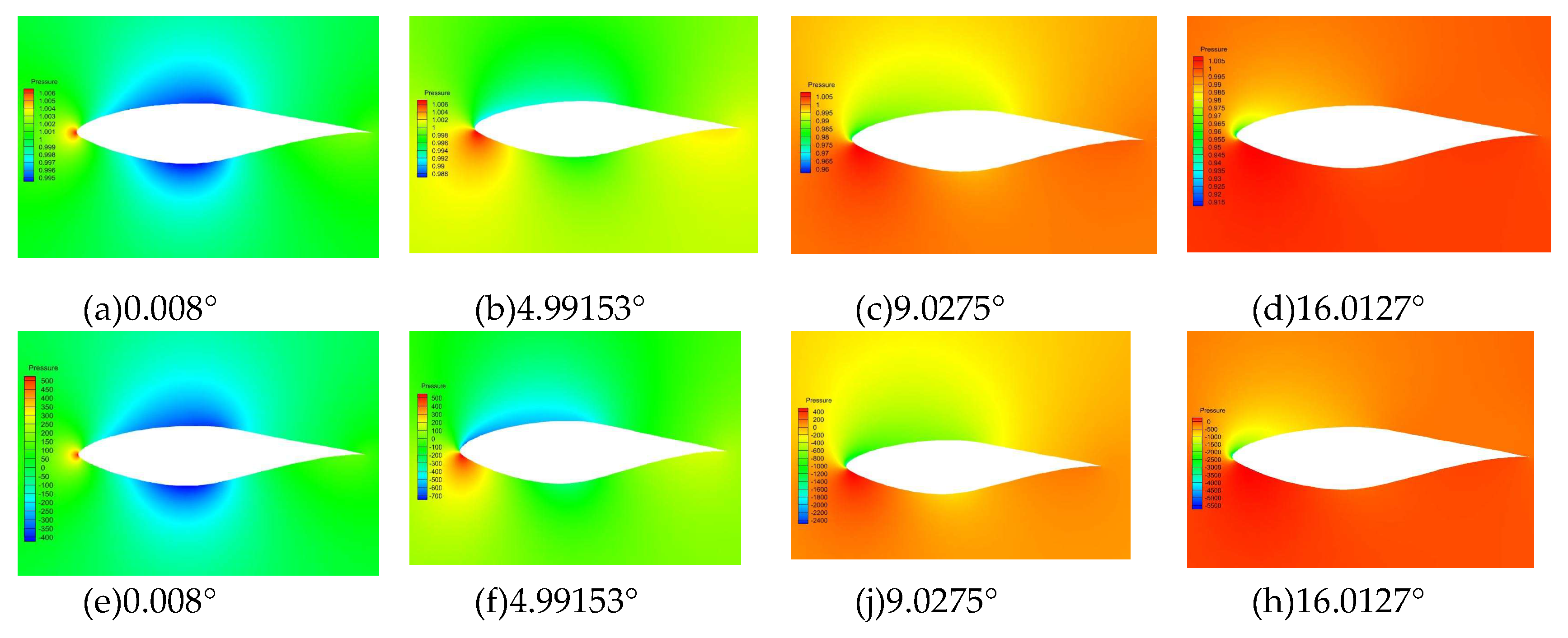
Figure 11.
Velocity Contour at different angle of attack by (a-d) Flow Numerical Solver ,(e-h) Ansys Fluent Solver.
Figure 11.
Velocity Contour at different angle of attack by (a-d) Flow Numerical Solver ,(e-h) Ansys Fluent Solver.
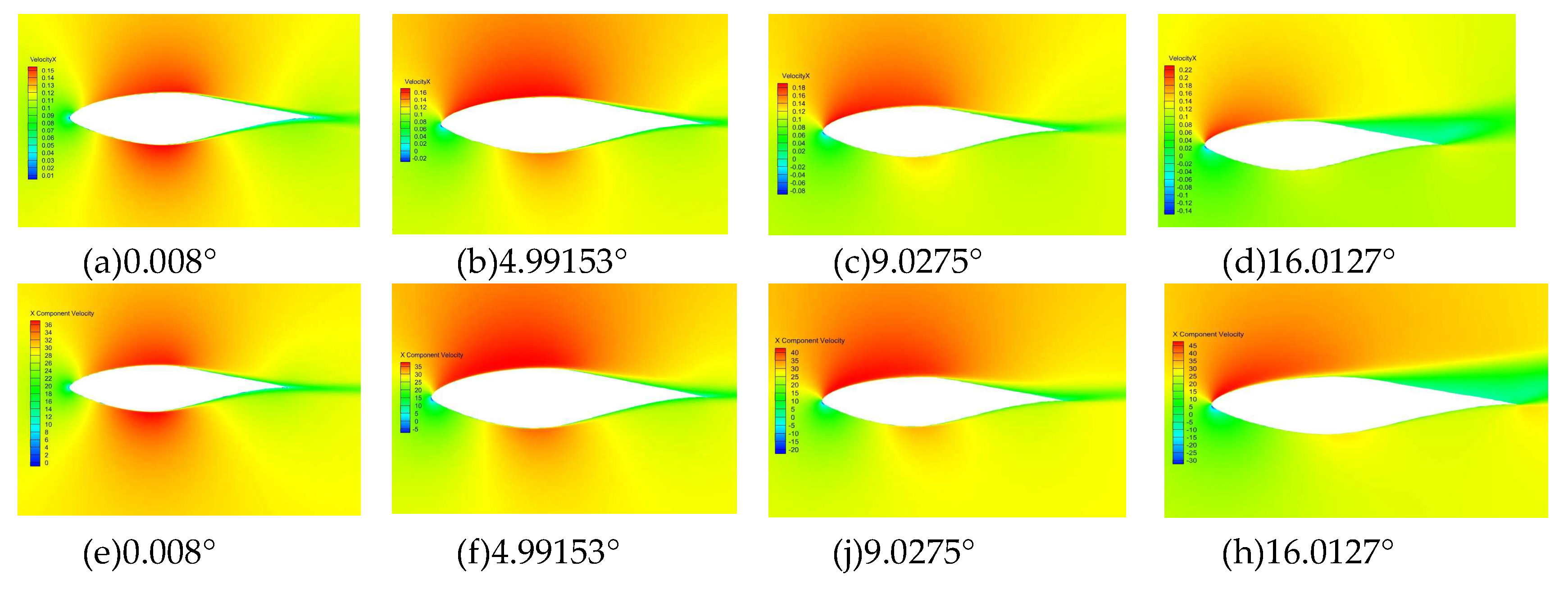
Figure 12.
Velocity Streamlines at Different Angles of Attack by (a-d) Flow Numerical Solver,(e-h) Ansys Fluent Solver.
Figure 12.
Velocity Streamlines at Different Angles of Attack by (a-d) Flow Numerical Solver,(e-h) Ansys Fluent Solver.
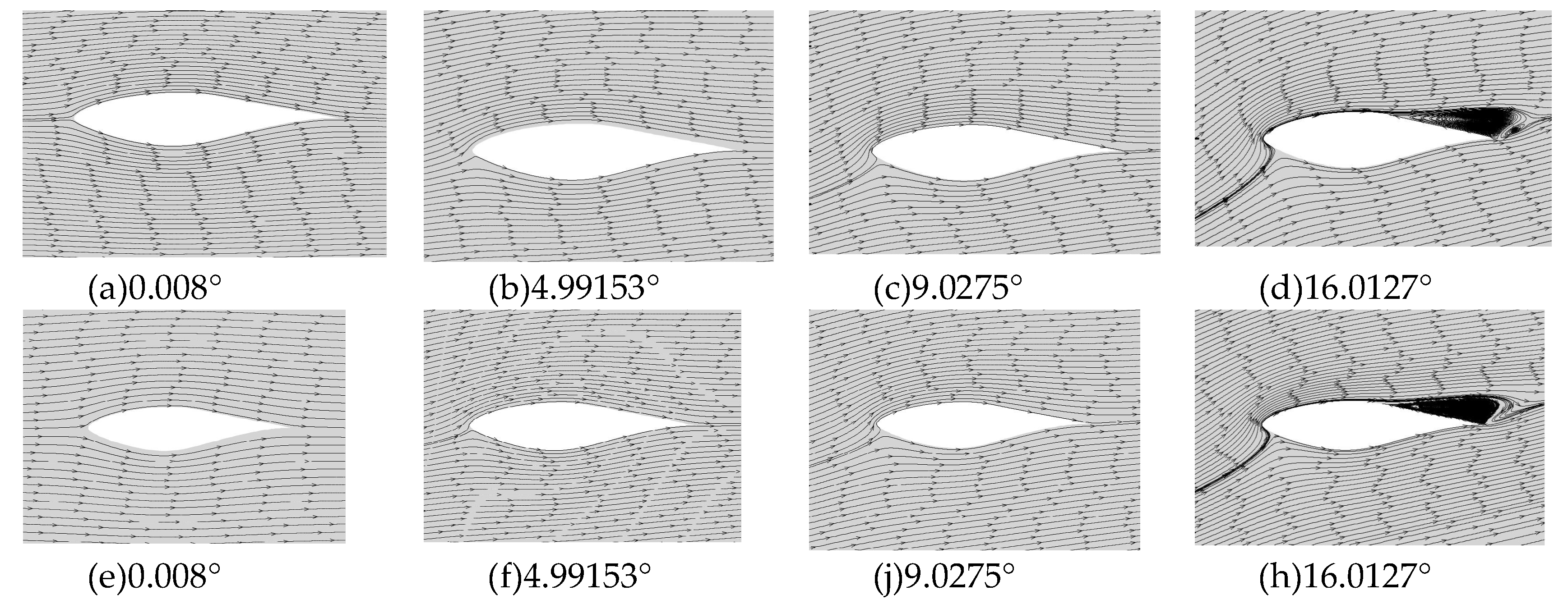
Figure 13.
Pressure Coefficient Distribution: Flow Numerical Solver vs Ansys Fluent Solver at Different Angle of Attack.
Figure 13.
Pressure Coefficient Distribution: Flow Numerical Solver vs Ansys Fluent Solver at Different Angle of Attack.
3.2. Airfoil Shape Optimization Design Result
This study presents solutions to the identified optimization challenges and critically evaluates their effectiveness. Our methodology encompasses a series of increasingly complex design iterations aimed at refining the airfoil contour. This refinement considers both the angle of attack and shape parameters across a range of wind velocities. Through this comparative analysis, we seek to enhance our understanding of airfoil shape optimization techniques, specifically focusing on the S809 Airfoil. For this purpose, we have developed a Free Form Deformation (FFD) model, as illustrated in Figure 4.b, and constructed the corresponding volume mesh, depicted in Figure 5.b. Detailed insights into this process are provided in Figure 2, which outlines SLSQP optimization methodology employed in our analysis.
As indicated in Table 2, I present the operational condition parameters selected for both single and three cases of multipoint optimization. Our discussion will begin by examining the results obtained from a single flow condition and will then progress to explore four distinct flow scenarios. In defining thermodynamic conditions, I have employed two distinct methodologies. The first approach involves parameters such as velocity, Reynolds number, Reynolds length, and temperature, while the second approach incorporates velocity, ambient pressure, and ambient temperature. It is worth noting that both approaches are applicable for low-speed flows. Additionally, supplementary quantities are determined using a foundational methodology
Despite the utilization of differing methodologies, our findings consistently demonstrate alignment. In the comprehensive study presented in the accompanying Table 3, the configuration parameters utilized in the optimization of the S809 airfoil shape are delineated, employing SLSQP method for effective optimization. The designated objective function was the minimization of the drag coefficient, meticulously modulated through FFD shape control variables alongside angle of attack adjustments. The optimization was subjected to an array of constraints, encompassing lift, geometric volume, and thickness specifications, Additionally, constraints are placed on the leading edge (LE) and trailing edge (TE) within the FFD box. These constraints are applied exclusively during the single-point and multipoint airfoil shape optimization processes. They ensure that corresponding points on the LE and TE are moved symmetrically, with each pair shifting by an identical measure but in reverse directions, to ascertain the airfoil’s aerodynamic viability and structural feasibility. A systematic augmentation in the complexity of design parameters was methodically executed, extending from a single-point optimization scenario to multiple-point considerations. This incremental complexity aimed to address a spectrum of operational flow conditions, each quantitatively characterized by distinct variables and constraints. Such an approach ensures a holistic optimization strategy, wherein the resulting airfoil configurations are anticipated to demonstrate enhanced aerodynamic efficiency within the defined operational envelope.
3.2.1. Single Point Optimization
This study examines a single point flow condition outlined in Table 2 and in Table 3 which summarizing the optimization problem aimed at minimizing the drag coefficient, involving 41 FFD design variables along with the angle of attack to control the airfoil shape, as depicted in Figure 4. There are 224 constraints in total including constraining the lift coefficient to be 0.4,keeping the local airfoil thickness between 0.85% and 1.25% of the baseline thickness, and ensuring the total volume of the optimized wing is at least equal to that of the baseline wing. Additionally, the leading and trailing edges of the wing are fixed. Where the Free-Form Deformation (FFD) displacement along the y-coordinate is confined within a range of ±0.5, and the angle of attack variable spans from 0 to 16 degrees.
Figure 14 shows the angle of attack design variable and drag coefficient convergence changes history for the optimization iteration .The outcomes demonstrate a decrease in thickness of about -8% and an increase in camber of approximately 18%, as detailed in Table 4, which also indicates a lift-to-drag ratio improvement of 22.25%. Figure 14.(a) demonstrates that the angle of attack changes only slightly during the optimization, suggesting its minimal impact on the results compared to optimizations that exclude it as a variable. Meanwhile, Figure 14.(b) shows that the performance measure (objective function) improves as the optimization iterations progress. In total, I conducted 29 adjoint computations and 59 flow solutions for the optimization
3.2.2 Multiple point optimization
In the previous scenario, it was demonstrated that single-point optimization fails to yield a design that performs satisfactorily across various operating conditions. Consequently, the motivation for employing multipoint optimization arises from the need to encompass a broader spectrum of flow conditions and achieve a more resilient design. In all optimization cases, a high-fidelity gradient-based optimization framework was employed. The design surface was parameterized using the Free-Form Deformation (FFD) method, while volume mesh deformation was managed through an analytic inverse-distance method. The computational fluid dynamics (CFD) simulations were conducted using an adjoint solver with the Spalart-Allmaras (SA) turbulence model.
For local airfoil shape control, 40 FFD control points were used, as shown in Figure 4. Additionally, the angle of attack was incorporated into the optimization for two, three, and four multipoint flight conditions, resulting in 42, 43, and 44 design variables, respectively. Lift coefficients were constrained for each flight condition, and the local airfoil thickness was maintained between 0.85% and 1.25% of the baseline thickness. The total volume of the optimized wing was required to be at least equal to that of the baseline airfoil, with fixed leading and trailing edges. This setup led to 225, 226, and 227 constraints being considered for each case of the multipoint optimization problem, as shown in Table 3. The operating flow condition optimization problem is presented in Table 2. SLSQP is used as the optimizer with accuracy tolerances set to 10-4. The optimizations run until the tolerances are met or the process aborts due to numerical difficulties.
The design optimization problem parameters and model remain consistent with those of single-point optimizations, albeit with adjustments made to the lift constraint and angle of attack design variable to accommodate the additional flow condition points. The convergence of the objective function history during the optimization iterations for the three flow conditions is apparent, as depicted in Figure 15.a, where the value of the objective function steadily decreases with progressing iterations, indicating effective modification of the airfoil’s shape and resulting in solutions that enhance the performance metric. Additionally, Figure 15.b illustrates the changes in the first angle of attack throughout iterations for two, three, and four multipoint scenarios, revealing a tendency for the angle to approach a minimum value as the number of points increases. Furthermore, with an increase in iteration count, the angle adjustment becomes more refined, signifying a convergence towards optimal solutions. From Figure 15, I can observe that increasing the number of points in the multipoint optimization also increases the number of iterations required to reach the optimal airfoil configuration.
4. Discussion
This study focuses on optimizing the 2D geometry of the S809 airfoil model, considering both single-point and multipoint configurations. To generate 3D meshes in CGNS format, I utilized a foundational methodology, producing meshes with a single cell width and applying symmetry boundary conditions on opposing faces to maintain the quasi-2D nature of the problem . As outlined in Table 4, the optimized airfoil profiles show variations depending on the operational parameters, leading to differences in thickness, maximum thickness location, camber, and maximum camber position. Notably, the optimized airfoils demonstrate a decrease in maximum thickness while shifting towards the leading edge, resulting in reduced drag force. Additionally, improvements in maximum camber and its relocation towards the leading edge enhance lift characteristics, leading to an increase in the lift-to-drag ratio.The aerodynamic coefficients ensuing from the single and multipoint optimization processes are comprehensively delineated in Table 5 I the reference airfoil configuration. These analyses, conducted at a Reynolds number of 3.48e6, illustrate discernibly augmented lift coefficients and cl/cd ratios for the optimized airfoils compared to the baseline S809 airfoil. Noteworthy enhancements in the lift-to-drag ratio, amounting to 22.5%, 22.2%, 21.4478%, and 21.544% for the single-point, two-point multipoint, three-point multipoint, and four-point multipoint optimized airfoils, respectively, further underscore the efficacy of the optimization process.
Next, I examine the shape and pressure (Cp) distributions for both the baseline and optimized geometries in Figure 16, focusing on both single and multipoint optimizations. The optimization process shows a reduction in thickness and a slight increase in camber from single to four-point optimization. This reduction in thickness is expected when prioritizing aerodynamics without considering structural strength constraints. The differences, particularly in thickness and camber parameters, align with Table 4, which indicates a blunt leading edge across all optimization cases. This feature makes the airfoil less sensitive to changes in wind speed and direction, ensuring more consistent performance under varying wind conditions. Additionally, it enhances durability and resistance to damage from debris, rain, and other environmental factors, reducing the risk of leading-edge erosion that can degrade aerodynamic performance over time. Furthermore, a blunt leading edge improves performance at lower wind speeds by delaying flow separation and maintaining smoother airflow over the surface, leading to a higher lift coefficient, which is beneficial for wind turbines in areas with variable wind conditions. A less sharp leading edge also helps reduce noise generated by the wind turbine blades, as sharper edges create more turbulence and higher noise levels. Furthermore, Figure 16.b illustrates the pressure distribution around the airfoil, indicating noticeable improvements resulting from the optimization process. Our simulations were conducted using the Intel i5-8500 CPU (3 GHz), revealing that increased design complexity leads to longer computational times, as evidenced by the significantly higher computational time for the four-point multipoint scenario.Consequent to CFD analyses performed via the Numerical flow field Solver across the entirety of the optimized airfoil configurations, including the baseline, within an angle of attack range spanning from 0 to 20 degrees, flow conditions were established with temperature and static pressure set at standard sea level conditions, specifically 288.15 K and 101325 Pa, respectively. These conditions align with typical operational parameters for wind turbines operating at altitudes not surpassing a few hundred meters. A Reynolds number of 3.48e6 was prescribed at a velocity of 51.48 m/s for all optimized airfoil configurations.
Figure 17 delineates improvements in lift coefficient, lift-to-drag ratio coefficient, drag coefficient, and moment coefficient. Particularly noteworthy is the discernible enhancement in lift-to-drag coefficient observed with the four-point multipoint optimization, especially evident up to an angle of attack of 12 degrees. Conversely, the single-point optimization exhibits superiority in terms of improvement in lift coefficient. Furthermore, Figure 17.c highlights the superior improvement afforded by single-point optimization in the context of lift coefficient.
In Figure 18, the lift-to-drag ratio is displayed for various wind turbine operating conditions, spanning velocities from 5 to 25 m/s and an angle of attack of 5 degrees. Utilizing the flow Numerica solver to demonstrate the lift to drag ratio for various optimization scenarios, including baseline, single-point, two-point, three-point, and four-point optimizations. It is evident that the lift-to-drag ratio improves as the number of optimization points increases, suggesting that multi-point optimization results in superior aerodynamic performance. The results indicate that the four-point optimized airfoil exhibits the highest lift-to-drag ratio across all velocities, showcasing superior overall performance compared to other optimization strategies. This demonstrates the advantages of utilizing advanced optimization techniques to enhance the aerodynamic efficiency of airfoils, a critical factor for the optimal performance of wind turbines within the designated velocity range.
5. Conclusions
This study successfully developed an efficient high-fidelity, RANS-based discrete adjoint method integrated within a constrained shape-design optimization framework, demonstrating its effectiveness through the optimization of the aerodynamic design of the NREL PHASE VI S809 Airfoil Rotor. The optimization framework comprises several key modules, including a geometric parameterization module utilizing Free-Form Deformations (FFDs), an inverse-distance method for volume mesh deformation, a flow simulation solver, a discrete adjoint solver for derivative computation, and a Sequential Quadratic Programming (SLSQP) method for nonlinear constrained optimization.
Through a comprehensive literature review on high-fidelity shape optimization in wind turbine design, this research identified a significant opportunity for advancement in this field. A comparative analysis of two advanced CFD solvers, Fluent and flow field numerical solver, demonstrated robust agreement with experimental data across a variety of angles of attack, validating the reliability of the simulation methods employed.
The study achieved notable results in airfoil optimization. A single-point optimization concerning angle of attack and FFD design variables led to an impressive enhancement in the lift-to-drag ratio by approximately 22.51%. Furthermore, multiple-point optimizations under the same constraints yielded significant improvements in lift-to-drag ratios of approximately 22.2%, 21.45%, and 21.54% for two, three, and four multipoint flow conditions, respectively. These advancements were primarily attributed to a strategic reduction in relative thickness and an increase in camber.
CFD analyses conducted across a range of angles of attack from 0 to 20 degrees for the optimized airfoil shape revealed that the four-point multipoint optimization produced the most substantial improvements in lift-to-drag ratio, lift coefficient, drag coefficient, and moment coefficient. These findings underscore the efficacy of the proposed optimization framework and highlight the potential for further advancements in aerodynamic design within the wind turbine sector.
In conclusion, this research contributes valuable insights to the field of aerodynamic shape optimization, presenting a robust methodology that can be applied to future studies and practical applications in wind turbine design. The demonstrated improvements in aerodynamic performance not only enhance the efficiency of wind turbine rotors but also pave the way for innovative approaches to optimizing complex aerodynamic systems.
Data: availability
This manuscript does not report data generation or analysis.
Ethics: approval and consent to participate
Not applicable.
Consent: for publication
Not applicable.
Author Contributions
Ajlan Jamal Ali Hussein: Data Curation, Conceptualization, Investigation, Methodology, Software, Validation, Visualization, Writing – Original Draft,Wenzhong Shen: Funding Acquisition, Supervision, Writing – Review & Editing Jiufa Cao: Conceptualization, Software, Writing – Review & Editing, Project Administration.
Funding
This research did not receive any external funding.
Acknowledgments
Not applicable.
Conflicts of Interest
The authors declare that they have no conflicts of interest.
References
- Agency, I.E. World Energy Outlook 2023 October 2023, 2023.
- Agency, I.R.E. Renewable Power Generation Costs in 2022; August 2023, 2023.
- REN21. What are the current trends in renewable energy. 2023. [Google Scholar]
- Ehrmann, R.S.; White, E.B.; Maniaci, D.C.; Chow, R.; Langel, C.M.; Dam, C.P.V. Realistic Leading-Edge Roughness Effects on Airfoil Performance. 31st AIAA Applied Aerodynamics Conference, 2013. [Google Scholar] [CrossRef]
- Khalil, Y.; Tenghiri, L.; Abdi, F.; Bentamy, A. Improvement of aerodynamic performance of a small wind turbine. Wind Engineering 2019, 44, 0309524X1984984. [Google Scholar] [CrossRef]
- Alpman, E. AIRFOIL SHAPE OPTIMIZATION USING EVOLUTIONARY ALGORITHMS.
- Della Vecchia, P.; Daniele, E.; DʼAmato, E. An airfoil shape optimization technique coupling PARSEC parameterization and evolutionary algorithm. Aerospace Science and Technology 2014, 32, 103–110. [Google Scholar] [CrossRef]
- Yassin, K.; Diab, A.; Ghoneim, Z. Aerodynamic optimization of a wind turbine blade designed for Egypt's Saharan environment using a genetic algorithm. Renewable Energy and Sustainable Development 2015, 1, 106–112. [Google Scholar] [CrossRef]
- Akram, M.T.; Kim, M.-H. Aerodynamic shape optimization of NREL S809 airfoil for wind turbine blades using reynolds-averaged navier stokes model—Part II. Applied Sciences 2021, 11, 2211. [Google Scholar] [CrossRef]
- Akram, M.T.; Kim, M.-H. CFD Analysis and Shape Optimization of Airfoils Using Class Shape Transformation and Genetic Algorithm—Part I. Applied Sciences 2021, 11, 3791. [Google Scholar] [CrossRef]
- Dina, A.; Dănăilă, S.; Pricop, M.V.; Bunescu, I. Using genetic algorithms to optimize airfoils in incompressible regime. INCAS BULLETIN 2019. [Google Scholar] [CrossRef]
- Ümütlü, H.C.A.; Kiral, Z. Airfoil shape optimization using Bézier curve and genetic algorithm. Aviation 2022, 26, 32–40–32–40. [Google Scholar] [CrossRef]
- Song, X.; Wang, L.; Luo, X. Airfoil optimization using a machine learning-based optimization algorithm. Journal of Physics: Conference Series 2022, 2217, 012009. [Google Scholar] [CrossRef]
- Nagawkar, J.; Ren, J.; Du, X.; Leifsson, L.; Koziel, S. Single- and Multipoint Aerodynamic Shape Optimization Using Multifidelity Models and Manifold Mapping. Journal of Aircraft 2021, 58, 1–18. [Google Scholar] [CrossRef]
- Zhang, Q.; Miao, W.; Liu, Q.; Xu, Z.; Li, C.; Chang, L.; Yue, M. Optimized design of wind turbine airfoil aerodynamic performance and structural strength based on surrogate model. Ocean Engineering 2023, 289, 116279. [Google Scholar] [CrossRef]
- Hansen, T. Airfoil optimization for wind turbine application. Wind Energy 2018, 21, 502–514. [Google Scholar] [CrossRef]
- Anitha, D.; Shamili, G.; Kumar, P.R.; Vihar, R.S. Air foil shape optimization using Cfd and parametrization methods. Materials Today: Proceedings 2018, 5, 5364–5373. [Google Scholar] [CrossRef]
- Du, X.; He, P.; Martins, J.R. Rapid airfoil design optimization via neural networks-based parameterization and surrogate modeling. Aerospace Science and Technology 2021, 113, 106701. [Google Scholar] [CrossRef]
- He, Y.; Agarwal, R.K. Shape optimization of NREL S809 airfoil for wind turbine blades using a multiobjective genetic algorithm. International Journal of Aerospace Engineering 2014. [Google Scholar] [CrossRef]
- Schramm, M.; Stoevesandt, B.; Peinke, J. Optimization of Airfoils Using the Adjoint Approach and the Influence of Adjoint Turbulent Viscosity. Computation 2018, Vol. 6. [Google Scholar] [CrossRef]
- Negahban, M.H.; Bashir, M.; Botez, R.M. Free-Form Deformation Parameterization on the Aerodynamic Optimization of Morphing Trailing Edge. Applied Mechanics 2023, 4, 304–316. [Google Scholar] [CrossRef]
- Lyu, Z.; Kenway, G.K.W.; Martins, J.R.R.A. Aerodynamic Shape Optimization Investigations of the Common Research Model Wing Benchmark. AIAA Journal 2015, 53, 968–985. [Google Scholar] [CrossRef]
- Kenway, G.K.W.; Martins, J.R.R.A. Multipoint Aerodynamic Shape Optimization Investigations of the Common Research Model Wing. AIAA Journal 2016, 54, 113–128. [Google Scholar] [CrossRef]
- He, P.; Mader, C.A.; Martins, J.R.; Maki, K.J. An aerodynamic design optimization framework using a discrete adjoint approach with OpenFOAM. Computers & Fluids 2018, 168, 285–303. [Google Scholar] [CrossRef]
- Lambe, A.B.; Martins, J.R.R.A. Extensions to the design structure matrix for the description of multidisciplinary design, analysis, and optimization processes. Structural and Multidisciplinary Optimization 2012, 46, 273–284. [Google Scholar] [CrossRef]
- Cho, T.; Kim, C. Wind tunnel test for the NREL phase VI rotor with 2 m diameter. Renewable energy 2014, 65, 265–274. [Google Scholar] [CrossRef]
- Anjuri, E.V. Comparison of experimental results with cfd for nrel phase vi rotor with tip plate. International journal of Renewable Energy Research 2012, 2, 556–563. [Google Scholar]
- Giguère, P.; Selig, M.S. Design of a Tapered and Twisted Blade for the NREL Combined Experiment Rotor. [CrossRef]
- Hand, M.; Simms, D.; Fingersh, L.; Jager, D.; Cotrell, J.; Schreck, S.; Larwood, S. Unsteady Aerodynamics Experiment Phase VI: Wind Tunnel Test Configurations and Available Data Campaigns. 2001. [Google Scholar] [CrossRef]
- Sederberg, T.W.; Parry, S.R. Free-form deformation of solid geometric models. SIGGRAPH Comput. Graph. 1986, 20, 151–160. [Google Scholar] [CrossRef]
- Chan, W.M.; Steger, J.L. Enhancements of a three-dimensional hyperbolic grid generation scheme. Applied Mathematics and Computation 1992, 51, 181–205. [Google Scholar] [CrossRef]
- Kenway, G.; Kennedy, G.; Martins, J.R.R.A. A CAD-Free Approach to High-Fidelity Aerostructural Optimization. 13th AIAA/ISSMO Multidisciplinary Analysis Optimization Conference, 2010. [Google Scholar] [CrossRef]
- Luke, E.; Collins, E.; Blades, E. A fast mesh deformation method using explicit interpolation. Journal of Computational Physics 2012, 231, 586–601. [Google Scholar] [CrossRef]
- Kraft, D. A Software Package for Sequential Quadratic Programming; Wiss. Berichtswesen d. DFVLR, 1988. [Google Scholar]
Figure 1.
Annual increase in power capacity for renewable energy[3].
Figure 1.
Annual increase in power capacity for renewable energy[3].
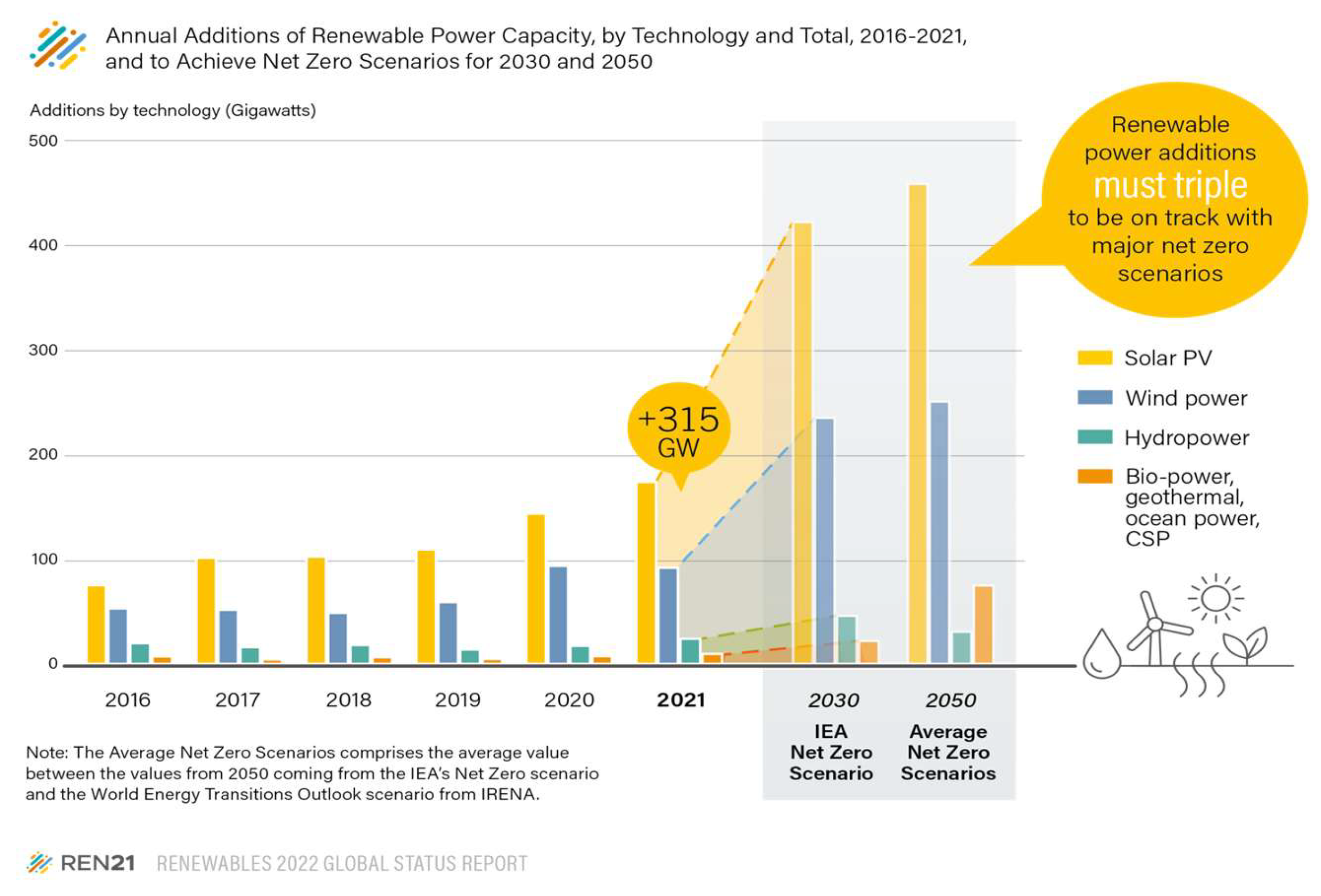
Figure 2.
Airfoil Shape Optimization Workflow.
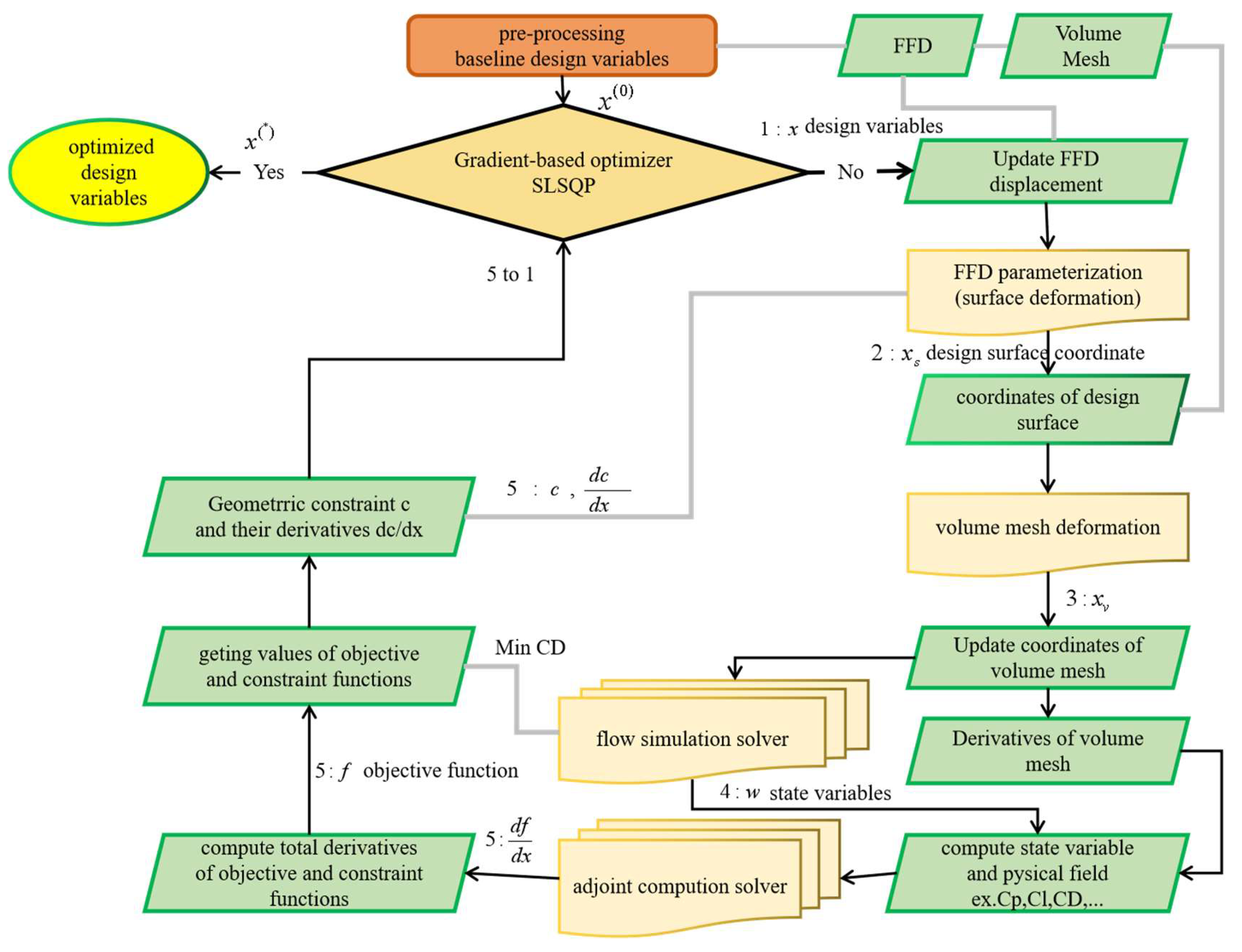
Figure 3.
Technical Drawing of a Blade shape of NREL Phase VI with airfoil S809.
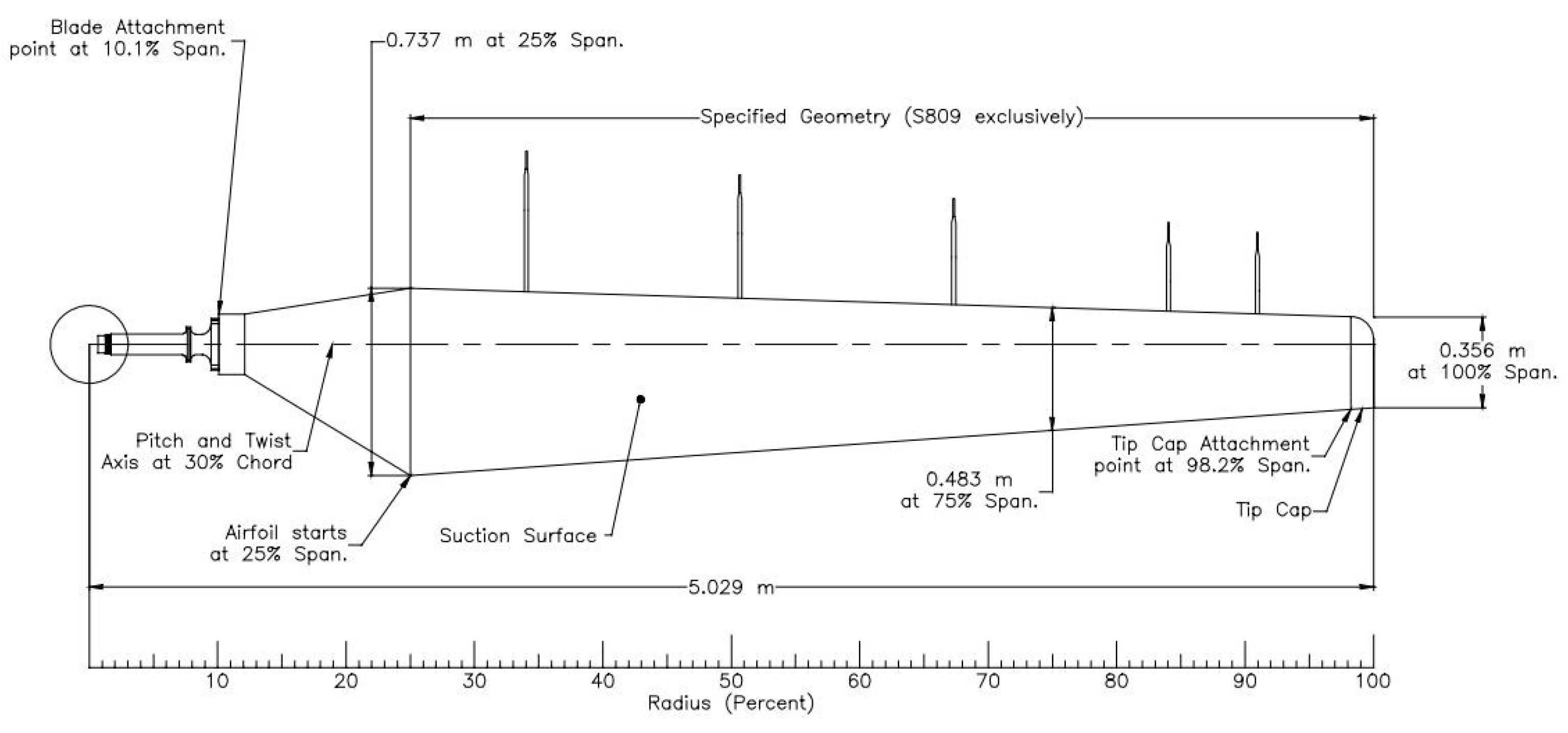
Figure 4.
FFD control points for S809 Airfoil.
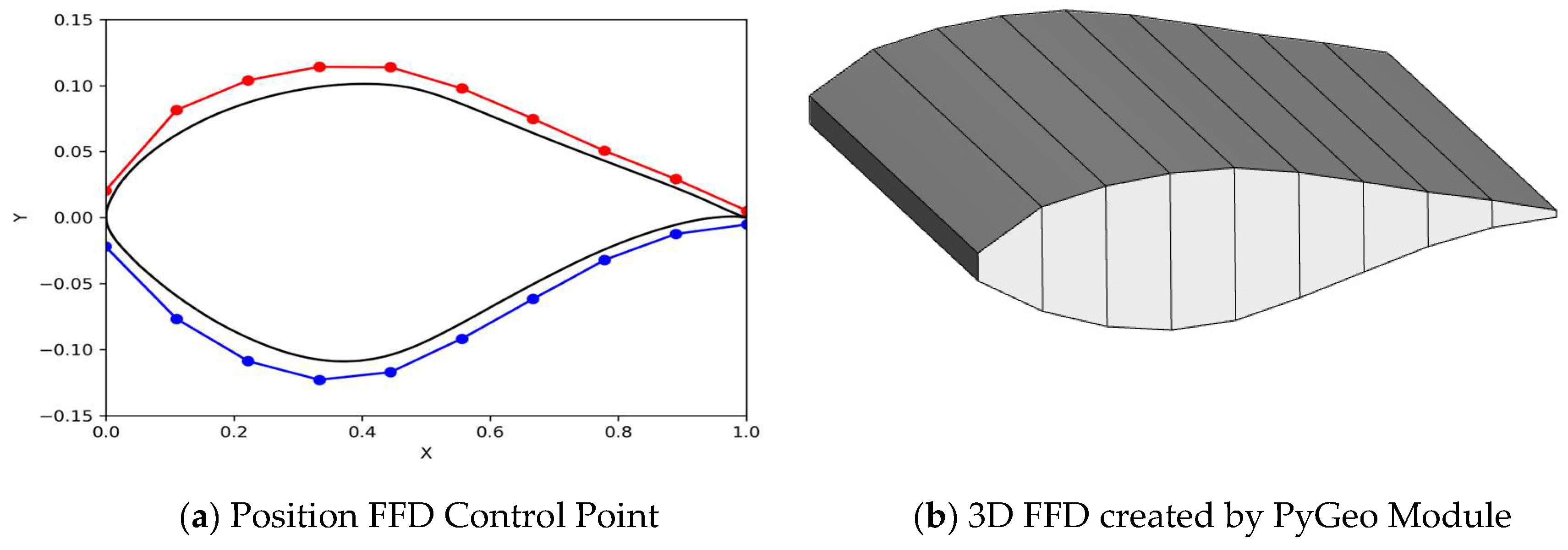
Figure 5.
Original S809 mesh generation.
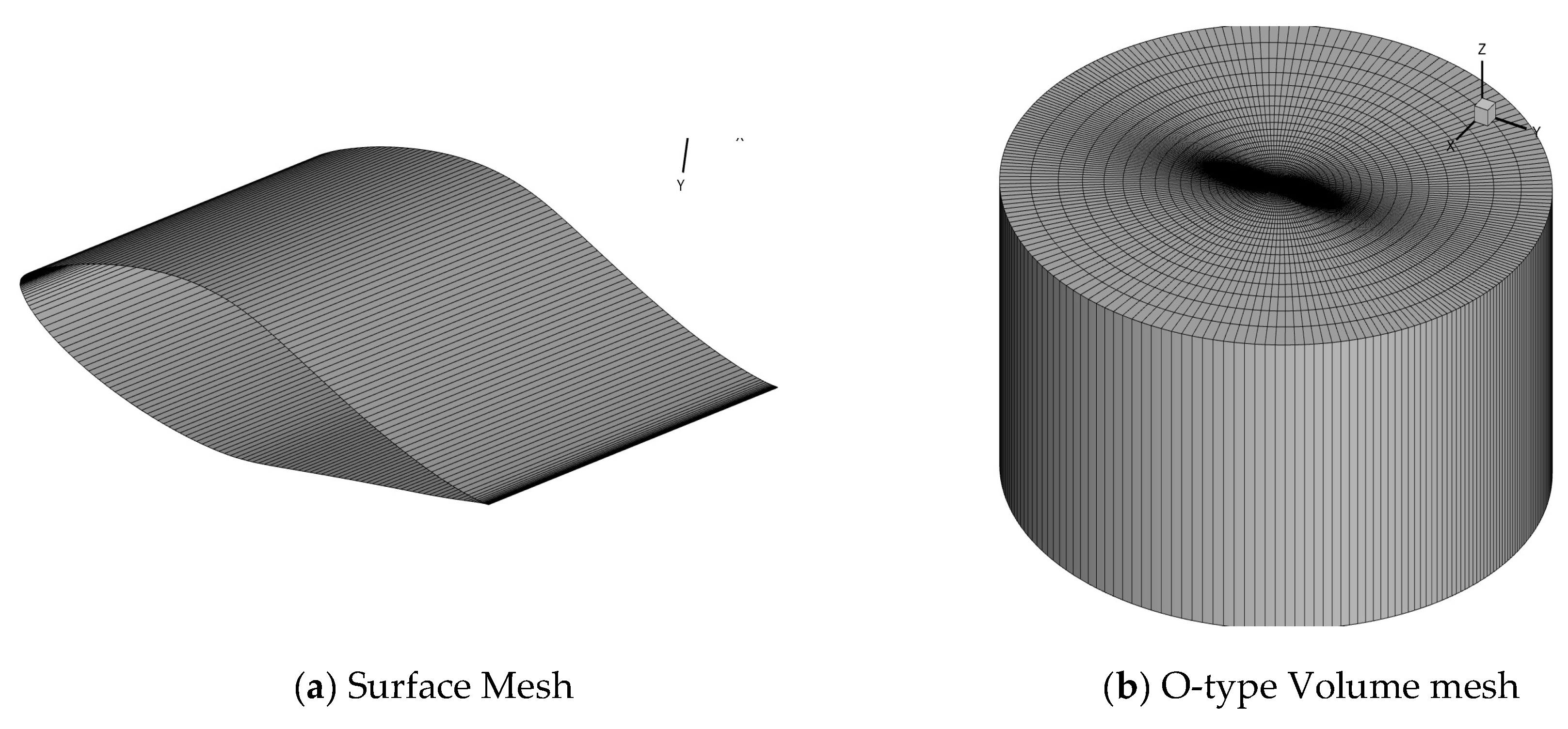
Figure 6.
Mesh Deformation of NREL S809 Airfoil.
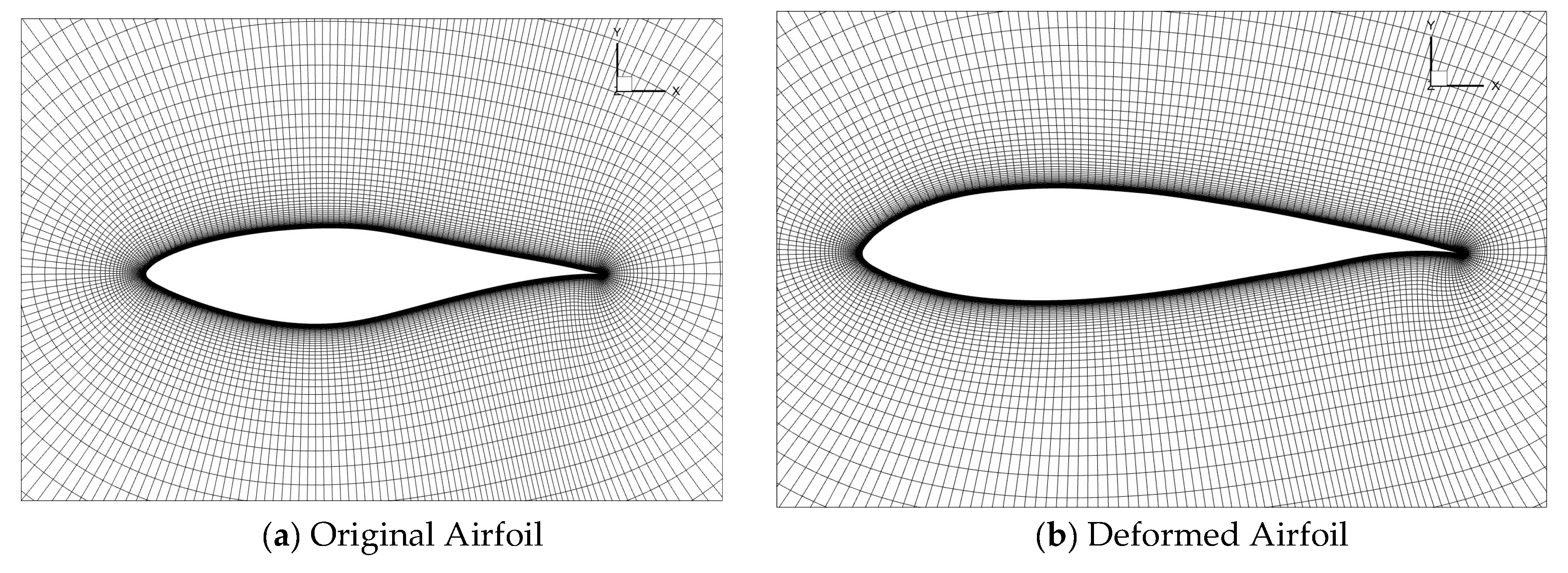
Figure 7.
Optimization process for aerodynamic shape.
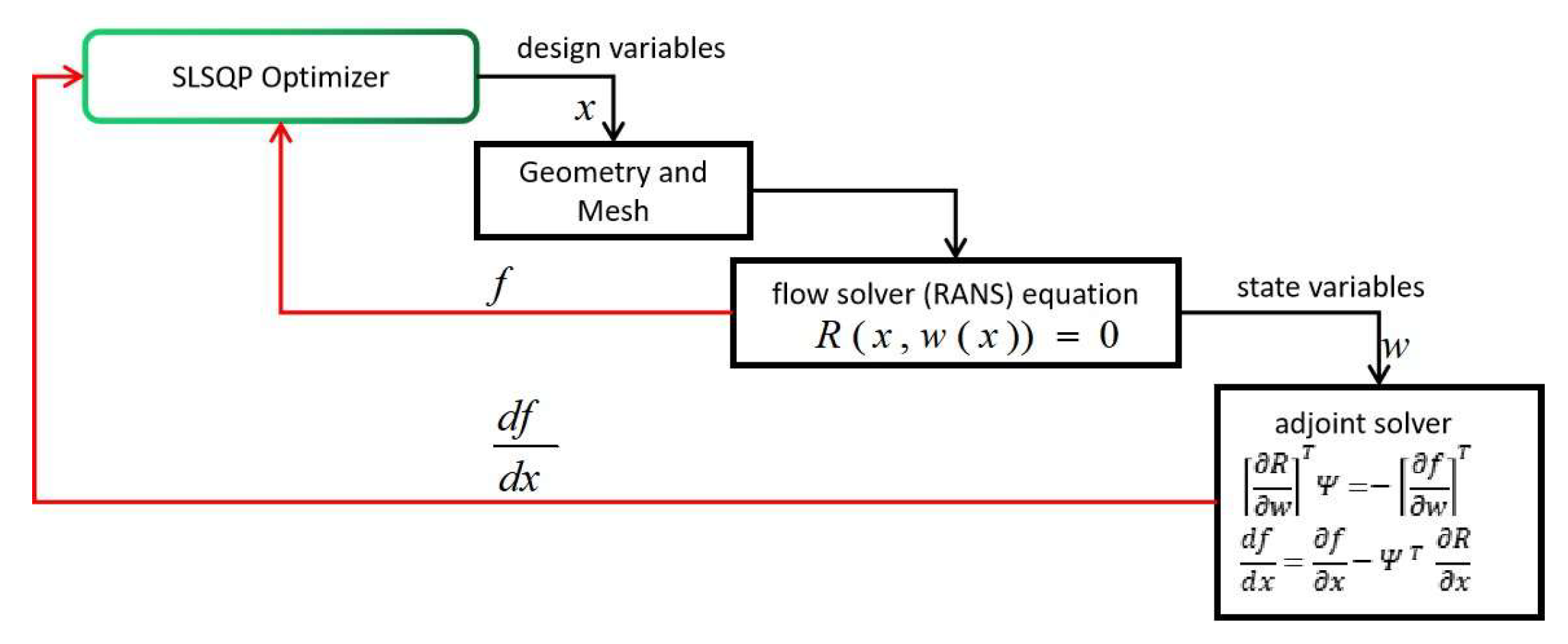
Figure 14.
Single-Point Shape Optimization During Iteration.
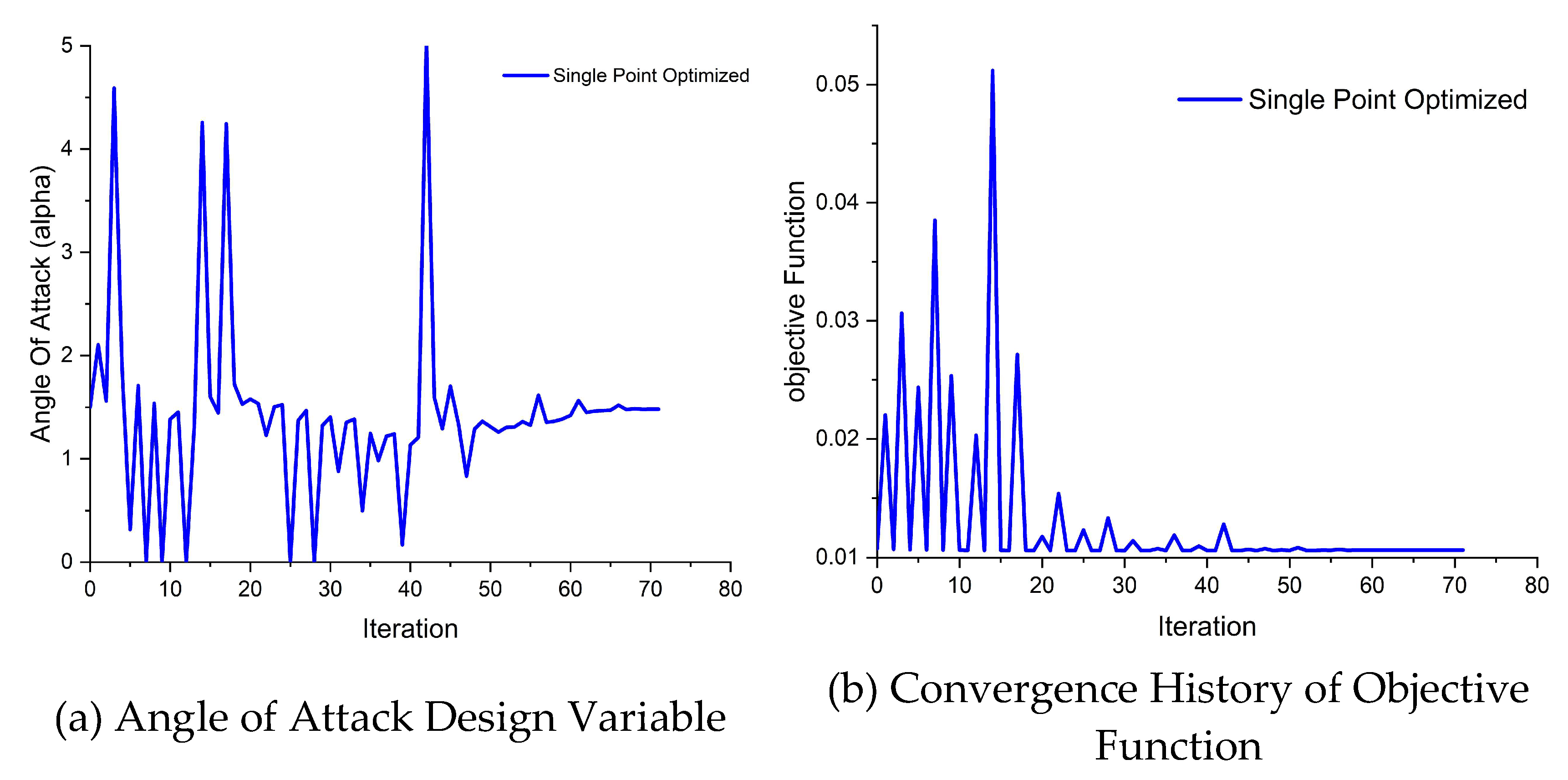
Figure 15.
History of Multiple Point Shape Optimization During Iteration.
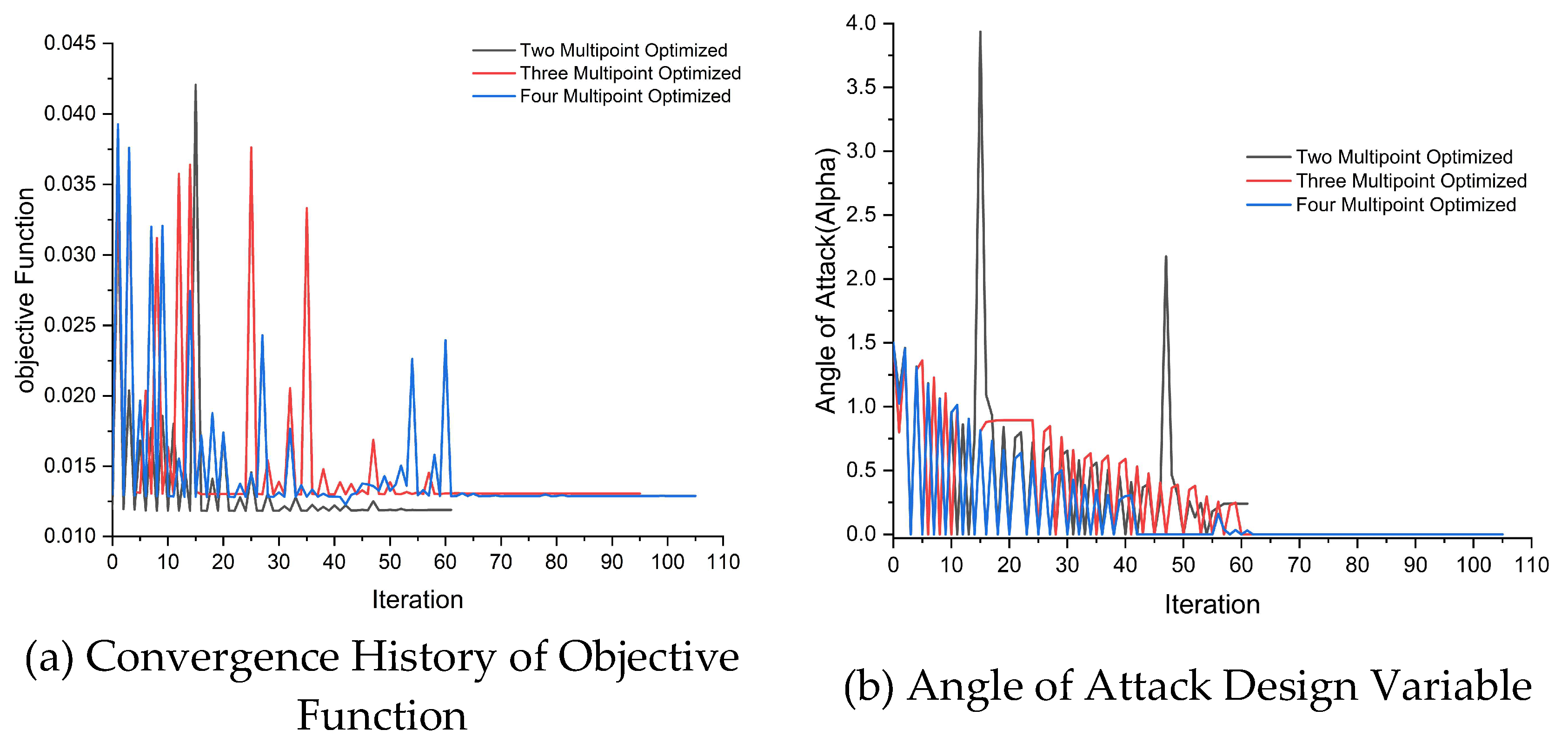
Figure 16.
Original and optimized at Re=3.48e6 for single and multiple point optimization.
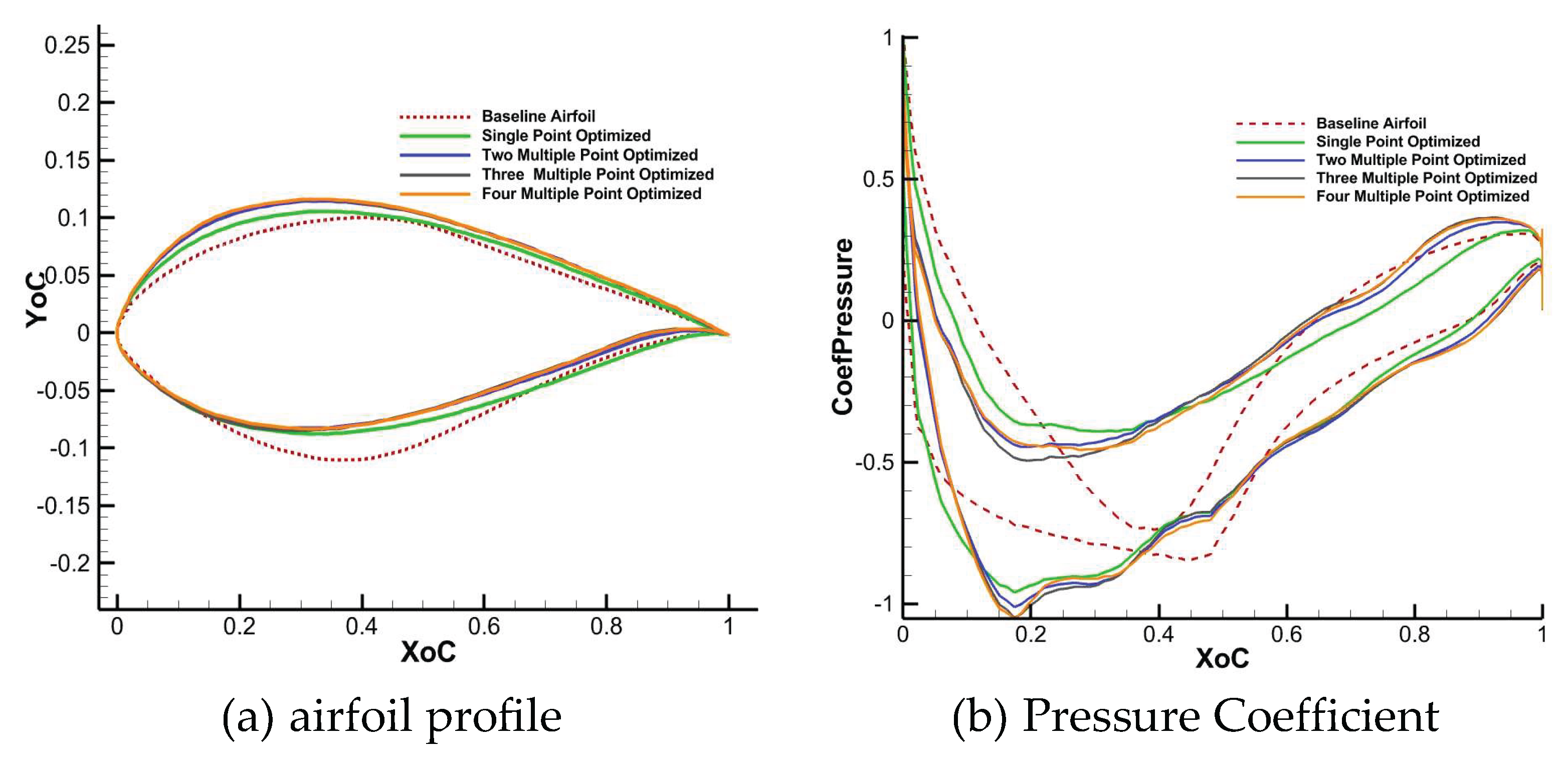
Figure 17.
Comparison Result of Original and Optimized at Re=3.48e6 for Single and Multiple Point Optimization.
Figure 17.
Comparison Result of Original and Optimized at Re=3.48e6 for Single and Multiple Point Optimization.
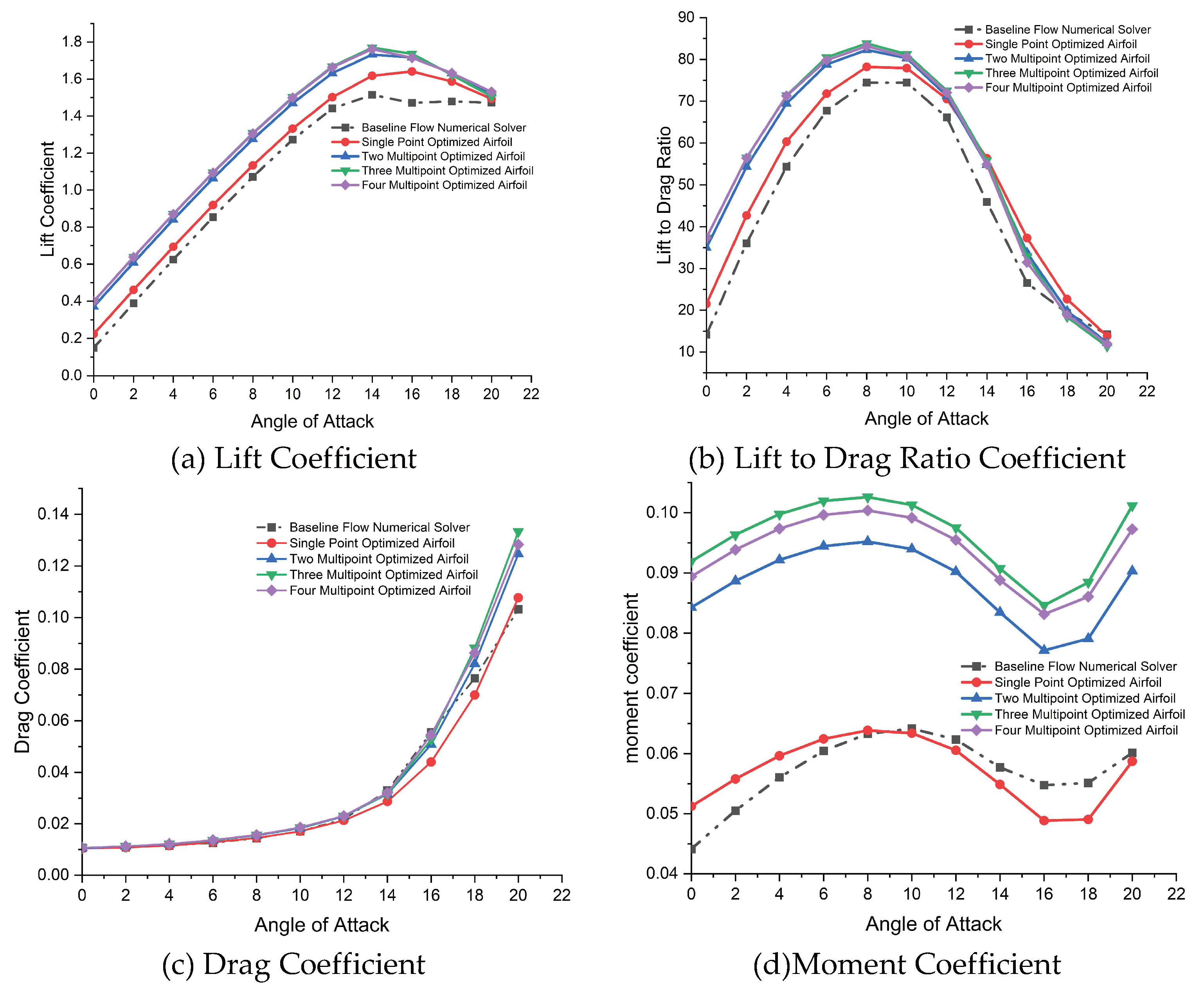
Figure 18.
Lift to Drag Ratio vs. Velocity for Different Optimized Result of S809 Airfoil at AOA= 5.
Figure 18.
Lift to Drag Ratio vs. Velocity for Different Optimized Result of S809 Airfoil at AOA= 5.
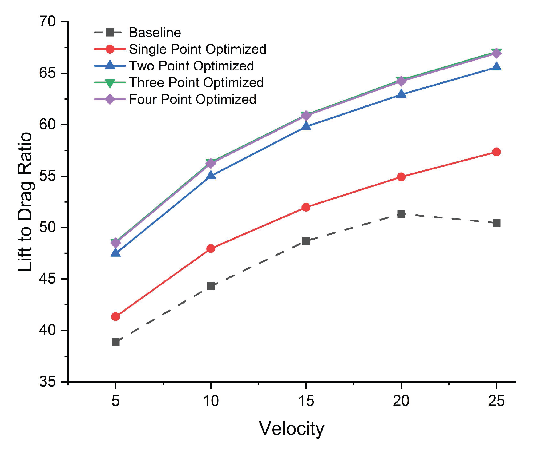

Table 1.
The geometry and design parameters of the NREL Phase VI rotor [29].
Table 1.
The geometry and design parameters of the NREL Phase VI rotor [29].
| Parameter | Symbol | Details |
|---|---|---|
| Rotor Diameter | D | 10.058 meters |
| No of Blade | Z | 2 blade |
| Tower hight | H | 12.192 m |
| Rotational speed | N | 72rpm |
| Cut-in wind speed | Vc | 5 m/s |
| Global pitch angle | 5o | |
| Cone angle | 0o | |
| Airfoil Type | NREL S809 | |
| Max Thickness | Lch | About 21% of chord length throughout the span |
| Blade chord | A linear taper (0.358–0.728 m) | |
| Twist Angle | Exhibiting non-linear twisting along its span (root =20.04 to tip =-2.5) | |
| Rated power | P | 19.8KW |
| Rotation direction | D | CCW |
| Purpose | Designed for Unsteady Aerodynamics Experiment and wind Energy research |
Table 2.
Operation Condition for single and multiple Point Optimization Problems.
| Flow Parameter Conditions | Single Point | Multiple Point Optimization | ||
|---|---|---|---|---|
| Two Point | Three Point | Four Point | ||
| Velocity of flow(V) | 51.48 | 51.48 ,29.214 | 51.48 , 29.214 , 14.16 | 51.48 , 29.214 , 14.16,43.822 |
| Angle of attack | 1.5 | 1.5,5.12 | 1.5, 5.12 , 6.12 | 1.5, 5.12 , 6.12,5 |
| Ambient Pressure | 101325 | 101325 | 101325 | 101325 |
| Reynold number Re | 3.48e6 | 3.48e6 , 2e6 | 3.48e6 ,2e6,1e6 | 3.48e6 ,2e6,1e6,3e6 |
| Ambient temperature (T) | 288.15 | 288.15 , 300.0 | 288.15 , 300,300 | 288.15 , 300,300,300 |
Table 3.
Overview of 2D aerodynamic shape single and multipoint optimization parameters.
| Objective Function | Description | Function/ Variable | Quentity | |||
| Single Point | Two Multipoint | Three Multipoint | Four Multipoint | |||
| Minimize | Average Drag coefficient | CD | ||||
| With respect to | surface shape variable | 40 | 40 | 40 | 40 | |
| Angle of attack | 1 | 2 | 3 | 4 | ||
| Total design variables | 41 | 42 | 43 | 44 | ||
| Subject to | Lift Constraint | 0.4 | [0.4 , 0.8] | [0.4,0.8,0.9] | [0.4,0.8,0.9,0.8] | |
| Geometric thickness constraint | 0.85t0 ≥ t ≥ 1.25t0 | 200 | 200 | 200 | 200 | |
| Geometric volume constraint | V ≥ V0 | 1 | 1 | 1 | 1 | |
| Fixed leading-trailing edge constraint | 2 | 2 | 2 | 2 | ||
| Design shape variable bounds | −0.05< ∆y < 0.05 | 20 | 20 | 20 | 20 | |
| Total constraints | 224 | 225 | 226 | 227 | ||
Table 4.
Airfoil Shape Optimization: Results of Geometric Parameters from Original, Single, and Multiple Point Optimizations.
Table 4.
Airfoil Shape Optimization: Results of Geometric Parameters from Original, Single, and Multiple Point Optimizations.
| Geometric Characteristics | S809 Airfoil | Single Point Optimized | Multiple Point Optimization | |||
|---|---|---|---|---|---|---|
| Two point | Three point | Four point | ||||
| Max. Thickness (%) | 21 | 19.3 | 19.71 | 20.01 | 19.92 | |
| Max. Thickness position (%) | 38.2 | 33.4 | 32.3 | 31.1 | 32.7 | |
| Max. Camber (%) | 0.82 | 0.98 | 1.72 | 1.82 | 1.78 | |
| Max. Camber position (%) | 81.9 | 50.5 | 63.3 | 65.6 | 64.6 | |
Table 5.
Performance result of single and multiple point optimization compared to Baseline at Re=3.48e6.
Table 5.
Performance result of single and multiple point optimization compared to Baseline at Re=3.48e6.
| Flow Characteristics | Single Point Optimized | Multiple Point Optimization | ||
|---|---|---|---|---|
| Two Point | Three Point | Four Point | ||
| AOA0iter-last | 1.5 – 1.4819 | 1.5 – 0.24033 | 1.5 – 1.96410-10 | 1.5 – 1.92710-11 |
| CL0iter-last | 0.32975 – 0.39999 | 0.329752 – 0.39999 | 0.329905 – 0.39999 | 0.329905 – 0.39999 |
| CD0iter-last | 0.010745 – 0.010637 | 0.010745-0.0106632 | 0.01072498 – 0.0107073 | 0.0107249 -0.0106985 |
| CL/CD0iter-last | 30.687 – 37.595 | 30.6875- 37.512 | 30.7605-37.358 | 30.7605-37.3875 |
| CL/CD improvement(%) | 22.5112 | 22.23867 | 21.4478 | 21.544 |
| Number of iteration | 71 | 61 | 95 | 105 |
| Computational time | 11.342 h | 10.5 h | 43.96 h | 53.22 h |
Disclaimer/Publisher’s Note: The statements, opinions and data contained in all publications are solely those of the individual author(s) and contributor(s) and not of MDPI and/or the editor(s). MDPI and/or the editor(s) disclaim responsibility for any injury to people or property resulting from any ideas, methods, instructions or products referred to in the content. |
© 2026 by the authors. Licensee MDPI, Basel, Switzerland. This article is an open access article distributed under the terms and conditions of the Creative Commons Attribution (CC BY) license (http://creativecommons.org/licenses/by/4.0/).
Copyright: This open access article is published under a Creative Commons CC BY 4.0 license, which permit the free download, distribution, and reuse, provided that the author and preprint are cited in any reuse.


