Submitted:
10 February 2026
Posted:
11 February 2026
You are already at the latest version
Abstract
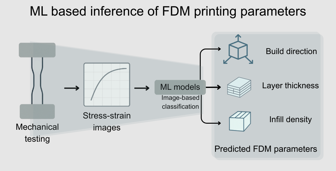
Fused Deposition Modeling (FDM) components require accurate identification of printing parameters to support reliable quality assessment and scalable reverse‑engineering workflows. This study evaluates whether mechanical response curves can be used to infer critical manufacturing parameters—specifically build direction, layer thickness, and infill density. Force–displacement and stress–strain data obtained from tensile tests were converted into image‑based representations and classified using individual and ensemble machine learning models. The influence of applying a moving‑average filter to smooth the curve‑derived images was also examined. Ensemble approaches, particularly AdaBoost, achieved higher accuracy and robustness across the evaluated variables, with the best results obtained from unfiltered stress–strain images. Under limited‑data conditions, ensemble models generally outperformed individual classifiers, while Multilayer Perceptron and Support Vector Machine models showed more stable but less accurate behavior. Overall, the findings demonstrate the feasibility of predicting FDM printing parameters directly from mechanical‑curve‑derived images, enabling a non‑destructive approach suitable for scalable reverse‑engineering and improved traceability within additive manufacturing processes.
Keywords:
fused deposition modeling
; mechanical testing
; mechanical-response-based classification
; printing parameters
; stress–strain images
; ensemble learning
1. Introduction
The evolution of manufacturing technologies in the context of Industry 4.0 has driven the adoption of more versatile and sustainable processes capable of meeting growing demand for complex parts, with reduced production times and superior mechanical properties [1]. Faced with these requirements, conventional methods such as machining have technical and economic limitations, which have boosted interest in additive manufacturing (AM) as a viable alternative for demanding industrial sectors [2].
AM encompasses various techniques that share a common principle: the layer-by-layer fabrication of three-dimensional geometries, with significant use of the base material [3]. The most widely used methodologies are Fused Deposition Modeling (FDM), which uses a molten thermoplastic filament; stereolithography (SLA), which uses a photopolymerized liquid resin; and Selective Laser Sintering (SLS), which sinters polymer powders using a high-powered laser [3]. These technologies are widely used across sectors such as automotive, aerospace, and biomedical, thanks to their ability to produce customized, functional components [4].
A critical aspect of AM is the sensitivity of the final product to printing conditions. Various studies have shown that parameters such as build orientation, layer thickness, and structural density significantly influence the mechanical properties obtained [5]. In particular, user-controllable parameters are essential, since parameters such as laser power or energy supplied are usually preconfigured in the system and cannot be easily adjusted [2]. In this context, multiple experimental studies have been conducted to quantify the effects of geometric and process variables on the mechanical strength of SLS-manufactured parts.
The characterization of mechanical properties in components manufactured using additive techniques requires specific tests, including tensile, compression, and flexural tests [6]. In particular, tensile tests allow force-displacement curves to be obtained from the continuous recording of the load applied to a test specimen and the corresponding displacement measured over a calibrated length [7]. These curves reveal critical information about the material's behavior, including the plastic zone, maximum force, breaking force, and yield point [8]. In addition, by knowing the cross-sectional area of the test specimen, it is possible to transform the curve into a stress-displacement diagram, which allows the determination of mechanical properties such as ultimate tensile stress and yield stress [9].
Despite their relevance for the design and validation of functional parts, conventional mechanical tests have operational limitations. First, they can take a long time depending on the loading speed and the type of material; second, they are inherently destructive, meaning the test specimen is lost after the test [10]. These conditions affect both the cost and efficiency of quality control processes, especially when working with large production volumes or high-cost materials. Given this scenario, it is necessary to use alternative methods to reduce the time and cost of these tests.
An emerging alternative to the limitations of conventional mechanical testing is the application of machine learning techniques to predict mechanical properties based on mathematical models [11]. Unlike finite element-based approaches, these models are highly computationally efficient, enabling implementation in remote environments, including cloud computing platforms [12]. Several studies have shown that specific algorithms can achieve highly accurate prediction metrics with significantly reduced resource consumption [13].
The integration of machine learning into the mechanical characterization stage has been shown to reduce the time and cost of physical testing while maintaining the reliability of the results [14]. Consequently, integrating 3D printing techniques with predictive algorithms provides a flexible, scalable framework for material evaluation, with significant potential in industrial and research applications.
Wang et al. [15] developed a long short-term memory (LSTM) model capable of predicting parameter configurations in engineering parts to meet specific stress-strain objectives. The model transforms the raw data into a format compatible with the LSTM, and it achieves a prediction accuracy of 0.8646 and a quadratic error of 0.1348 in inverse prediction tasks. These results show that further research is warranted.
Similarly, Tiwari et al. [16] conducted research to implement machine learning models, such as Support Vector Machines (SVM), Artificial Neural Networks (ANN), and Random Forest (RF), among others, to provide support throughout the design process of the mechanical parts to be manufactured. It is noteworthy that Two-stream Convolutional Neural Networks (CNNs) are particularly adept at predicting part stress based on the specified parameters, whereas the SVM model is the optimal choice for recommendations concerning design characteristics and printing parameters.
On the other hand, Ulkir et al. [17] integrated artificial intelligence systems with additive manufacturing (AM) to reduce the manufacturing time and cost of 3D-printed mechanical parts using the raster angle parameter. The optimal value of this parameter depends on the product's geometry, and changing it alters the stress distribution throughout the part. They used models such as SVM, Gaussian Process Regression (GPR), an ANN, Decision Tree Regression (DTR), and RF regression to estimate the optimal raster angle. Training data with different geometries and shapes was generated, and the models were trained in MATLAB. Ultimately, RFR produced the best results, with an R-squared value of 0.93, an explained variance score of 0.93, a root mean square error of 0.056, and a mean squared error of 0.0032. This model ensures optimal raster angle values for any geometry.
Rezasefat et al. [18] developed two deep learning architectures, MUDE-CNN and MTED-TL, to predict the evolution of the stress field in complex 3D structures fabricated via additive manufacturing (AM), particularly around defects such as isolated pores. The researchers trained their models using full-scale finite element simulations and designed them to capture temporal and spatial stress evolution. The MTED-TL architecture employed progressive transfer learning across encoder-decoder blocks and achieved higher prediction accuracy than the MUDE-CNN architecture. Additionally, they implemented an autoregressive training framework, which further enhanced temporal predictions. These approaches enable real-time monitoring and proactive defect mitigation during fabrication, improving the structural integrity and reliability of AM-produced components.
Wu et al. [19] conducted a critical review of residual stress prediction in laser additive manufacturing (LAM), focusing on its impact on industries such as aerospace, automotive, and biomedicine. Residual stresses, induced by thermal gradients during fabrication, can cause distortions or cracking in printed parts, so accurately predicting them is essential. The authors explored various approaches, including experimental techniques, computational simulations, and machine learning models. These approaches contribute to a deeper understanding of stress formation and mitigation. The review also identified current challenges and proposed strategies to enhance prediction accuracy and manufacturing reliability in LAM applications.
For this work, it is proposed to determine FDM parameters based on the mechanical properties observed in the force-displacement (or stress-strain) curves of manufactured parts. This approach is a form of reverse engineering aimed at replicating the function of components. At this stage, three geometric variables are considered: build direction, layer thickness, and infill density (see Figure 1).
Figure 2 presents a general outline of the methodology used in this research. Each stage will be described in detail in the following section.
2. Materials and Methods
2.1. Test Specimen Printing and Data Collection
The test specimens were manufactured in accordance with ISO 527-2 type 1A [20] (Figure 3a) using glass fiber-reinforced PLA material in a 3D printer Flashforge Adventurer 4, varying the layer thickness (0.1 or 0.2 mm), the build orientation—horizontal (build plane aligned with the machine X–Y plane) or vertical (build direction aligned with the machine Z-axis), and infill percent (60 or 100%). The tensile test was performed on a Tensile Shimadzu machine (see Figure 3b).
2.2. Data Processing
The data obtained from the mechanical tests were purified to remove unrepresentative information introduced by the fracture of the test specimens. The moving average method involved calculating the mean of a data window, which was then used as a reference point to identify outliers. It was determined that points that exceeded a standard deviation threshold from the mean should be truncated, along with the subsequent records. In this study, both the unrefined data and filtered versions were evaluated, using thresholds of 3 and 5 standard deviations as truncation criteria. Figure 4 shows Force-Displacement and Stress-Strain graphs before and after treatment, with a moving average of 3 standard deviations.
For model training, visual representations were used instead of raw numerical data to mitigate biases arising from data-collection variability [21,22,23,24,25]. This variability originated in experimental conditions, as test specimens with different layer heights, densities, and build orientation were used, which led to variations in test duration and, consequently, in the amount of data obtained for each sample.
2.3. Learning Models and Hyperparameter Tuning
The present study employed eight widely used classification algorithms, which have been employed in numerous related studies. DecisionTreeClassifier (DTC), AdaBoostClassifier (ABC), Support Vector Machines (SVM), Multilayer Perceptron (MLP), RandomForestClassifier (RFC), GradientBoostingClassifier (GBC), LogisticRegression (LR), and ExtraTreesClassifier (ETC) [26,27,28]. The selection of these models was based on their proven effectiveness in supervised classification tasks and their ability to handle datasets with structural characteristics similar to those in the present study.
A StratifiedKFold cross-validation with 30 splits was applied, ensuring class balance in each partition. In every iteration, about 96.7% of the data was used for training and 3.3% for validation, so that each sample served once for testing and multiple times for training. Using this scheme, hyperparameters were optimized through Bayesian optimization with the Optuna library, which evaluated candidate configurations, computed the performance metrics (accuracy, f1, recall, roc_auc) across the folds, and selected the best configuration based on the mean roc_auc.
3. Results
3.1. Build Direction
Once the images corresponding to the force–displacement and stress–strain graphs in the selected training and testing models had been processed and loaded, and the hyperparameters had been adjusted using Bayesian optimization with the Optuna library, the performance evaluation metrics were applied. The accuracy results obtained are presented in Table 2.
In the classification by build direction, the Gradient Boosting Classifier (GBC) achieves the highest accuracy with the ESM filter (without moving-average smoothing), reaching values close to 0.74, suggesting that preserving the original signal without smoothing treatment may be beneficial for classification, as it preserves critical information that could be lost during filtering. Likewise, the AdaBoost Classifier (ABC) and the Random Forest Classifier (RFC) achieve competitive performance in the EM5 and ESM scenarios, respectively, due to their ensemble-based approaches, which combine multiple base estimators and are less prone to systematic errors than individual models. By contrast, the Multilayer Perceptron (MLP) model produced results with a lower standard deviation, suggesting greater consistency; however, its overall accuracy was lower. Conversely, while the GBC and RFC models achieved acceptable accuracy values, they exhibited greater variability, potentially indicating less stability when faced with changes to the applied filters.
In general, the results suggest that both the graph type (with better performance in stress-strain curves) and the treatment applied to the images significantly affect the models' accuracy. Avoiding excessive filtering can improve classification by preserving the spectral richness of the original signal.
Table 3 shows the results for the F1 score, which balances precision and recall by evaluating the model's ability to detect positive cases while avoiding false positives. In this case, the AdaBoost Classifier (ABC) model achieved the highest average F1-score, exceeding 0.75, in the FM5 configuration (a moving average with five standard deviations). This was accompanied by a lower standard deviation, indicating high performance stability.
Models such as the Gradient Boosting Classifier (GBC) and the Random Forest Classifier (RFC) also showed favorable results in configurations such as ESM and FM3, though with higher variability. For its part, the Multilayer Perceptron (MLP) model recorded the lowest F1 scores, in some cases below 0.40 (as in FSM and FM3), suggesting limited ability to extract relevant patterns from the images and considerable standard deviation, indicating inconsistent predictions.
The Decision Tree Classifier (DTC) model performed intermediate, with an F1 score of 0.699 in the EM3 configuration. However, there was a significant drop in performance under other conditions, such as ESM, suggesting that the model is sensitive to the preprocessing method.
Table 4 presents Recall metric results, reflecting each model's ability to correctly detect positive cases. In this context, the AdaBoost Classifier (ABC) model stands out with the highest average values, close to 0.91 in the EM3 and FM5 configurations, accompanied by a low standard deviation, indicating high consistency in its performance.
Conversely, the Gradient Boosting Classifier (GBC) and Random Forest Classifier (RFC) models also produce favorable results, averaging between 0.73 and 0.76, though this varies moderately depending on the filter applied. Models such as the Support Vector Machine (SVM), the Extra Trees Classifier (ETC), and the Logistic Regression (LR) yield acceptable results across different configurations; however, their high standard deviations limit the reliability of their predictions.
Once again, the Multilayer Perceptron (MLP) model shows the lowest performance, with values close to 0.26 in the EM5 condition and high dispersion in almost all filters, demonstrating a limited ability to detect positive cases. Finally, the Decision Tree Classifier (DTC) model shows intermediate performance, with good results on EM3 and FM5, but is highly sensitive to preprocessing type, which affects its consistency.
Table 5 presents the mean ROC AUC values, which evaluate the models' overall performance across different decision thresholds and provide a comprehensive view of their discriminatory capacity. In this context, the highest values were obtained by the AdaBoost (ABC) and GradientBoosting (GBC) models, both averaging 0.7417 under the ESM filter, demonstrating the models' high sensitivity and robustness after preprocessing. Similarly, the Decision Tree (DTC) models with EM5 and the Gradient Boosting (GBC) model with FSM achieved values of 0.7333, confirming their effectiveness in complex, challenging environments.
In contrast, the MLP and SVM models showed more modest performance, with averages ranging from 0.55 to 0.63 across most filters, reflecting difficulties in capturing discriminative patterns in this task. However, MLP with EM5 exhibited the lowest standard deviation of the set (0.196), indicating relatively stable behavior despite its lower effectiveness.
To complement the values presented in Table 2, Table 3, Table 4 and Table 5, box plots are included for each metric and model (see Figure 5). These aim to facilitate the identification of patterns of dispersion and variability between models. This representation provides additional insight into values that differ from the mean, enriching the interpretation of the results. It is also possible to observe outliers in specific configurations, which could reflect differences in model reliability, likely associated with data processing.
In addition to the statistical summaries, heatmaps were generated to provide a consolidated visual overview of model performance across all metrics and filter configurations (see Figure 6). By encoding values through a continuous colour scale, this representation enables swift identification of areas of higher or lower performance, revealing consistent trends and highlighting contrasts that may be less evident in numerical tables. The side-by-side arrangement of heatmaps for each configuration is an effective method to facilitate cross-comparison. This approach provides an immediate, intuitive understanding of how models behave under different experimental conditions.
These results were compared with those of Barrios et al. [33], who used decision tree-based models to predict the roughness of parts manufactured by fused deposition modeling (FDM) in two build directions: Ra, 0°, and Ra, 90°. In their study, the Decision Tree model (J48/C4.5) achieved accuracies of 0.709 and 0.733, respectively, in each direction, while Random Forest reported accuracies of 0.807 and 0.743. In this study, Random Forest with the ESM filter achieved an accuracy of 0.70, an intermediate value between the two angles reported by Barrios et al. Meanwhile, DTC achieved an accuracy of 0.720 with EM5 preprocessing, DTC but decreased to 0.610 with ESM, demonstrating the significant sensitivity to image processing methods.
In the current study, the FM5 filter yielded an F1 score of 0.680 for Ra,0°, compared with the 0.716 reported by Barrios et al. for the same orientation. Under EM3 preprocessing, the DecisionTree model achieved an F1 score of 0.690, surpassing the 0.650 documented by Barrios et al. With respect to ROC AUC, Barrios et al [33]. obtained 0.692 and 0.481 for Random Forest in Ra,0° and Ra,90°, respectively; in contrast, the present work's Random Forest ROC AUC ranged from 0.630 to 0.730 depending on the chosen filter. For the DecisionTree classifier, Barrios et al. [33] reported ROC AUC values of 0.154 and 0.385, whereas this investigation observed values ranging from 0.610 to 0.760 across different preprocessing methods.
The key difference between the two studies is the origin and volume of the data used. Barrios et al. based their work on five clean numerical variables. In contrast, this study analyzed force-displacement and stress-strain curves from images subjected to different moving-average filters. This study also optimized hyperparameters with Optuna. These factors were shown to have a decisive impact on the final metrics.
On the other hand, Patil et al. [34] classified the need for support in FDM parts as being implicitly related to the printing direction. In their study, Random Forest achieved an accuracy of 0.88, an F1 score of 0.87, a recall of 0.87, and an ROC AUC of 0.87. In contrast, this study's results showed that the same model achieved 0.73 in accuracy (EM5), 0.68 in F1 score (FM5), 0.76 in recall (FM5), and 0.71 in AUC (ESM). Patil et al. reported an accuracy of 0.90, F1 score of 0.90, recall of 0.90, and AUC of 0.90 for the decision tree model. In this study, the decision tree model yielded an accuracy of 0.69 (FM5), an F1 score of 0.69 (EM3), a recall of 0.76 (EM3), and an AUC of 0.73 (EM5). For SVM, Patil et al. obtained an accuracy of 0.69, an F1 score of 0.65, a recall of 0.69, and an AUC of 0.66. In our study, SVM achieved an accuracy of 0.62 (EM3), an F1 score of 0.64 (ESM), a recall of 0.71 (EM3 and ESM), and an AUC of 0.675 (ESM). For Gradient Boosting, Patil et al. achieved an accuracy of 0.89, an F1 score of 0.89, a recall of 0.89, and an AUC of 0.88. In this study, the model achieved an accuracy of 0.73 (ESM), an F1 score of 0.70 (EM3), a recall of 0.73 (EM5), and an AUC of 0.74 (ESM).
These discrepancies can be explained by the fact that Patil et al. used thirteen clean, wall-based numerical variables whose characteristics directly affect support prediction. In contrast, force-displacement and stress-strain curves were processed using filtering and conversion to image and matrix formats. During these stages, critical data necessary for classification is lost.
3.2. Layer Thickness
Table 6 presents the classification accuracy per model and filter for the Layer thickness parameter. The AdaBoost Classifier (ABC) model achieves the highest average value (0.672) in the ESM configuration, with a low standard deviation. This behavior suggests that keeping the image unchanged by moving average could benefit the classification by preserving critical information that could be lost during filtering. Likewise, the ABC model shows acceptable performance in the FM3 and FM5 configurations, demonstrating good stability across different transformations.
The Decision Tree Classifier (DTC) model also shows favorable results, with average scores close to 0.59 across most scenarios. However, it exhibits greater dispersion, which could indicate an adequate ability to extract relevant patterns, although with high sensitivity to the type of processing applied.
The Gradient Boosting Classifier (GBC) and Random Forest Classifier (RFC) models report intermediate accuracy values, but with higher standard deviations than other models, suggesting a clear dependence on the filter used. On the other hand, the Multilayer Perceptron (MLP) model yields relatively low values, albeit with low deviation, suggesting less accurate but more consistent behavior.
Finally, the Support Vector Machine (SVM) and ExtraTrees Classifier (ETC) models show less favorable results, with configurations achieving an accuracy of no more than 0.43. In general, ensemble models—particularly those based on boosting—perform better on this classification task.
On the other hand, Table 7 shows the F1-score values, aiming to achieve the best balance between precision and recall. In this case, the AdaBoost (ABC) model again yielded the highest average values, with a mean of 0.7089 across both the FM3 and FM5 filters and a low standard deviation. It should be noted that the Multilayer Perceptron (MLP) also offered outstanding results in FM3 and FM5, with values above 0.6. In contrast, the ExtraTrees Classifier (ETC) and Random Forest Classifier (RFC) models had the lowest values, with average F1-scores below 0.45 and high dispersion. The Logistic Regression (LR) and Support Vector Machine (SVM) models yielded intermediate values, with EM5 and FSM standing out, respectively. The Decision Tree (DT) model achieved its highest value (0.576) in the ESM filter, although with a high standard deviation.
Table 8 shows the recall values for each model under each applied filter. The MLP and AdaBoost (ABC) models achieved the highest average values, particularly when using the FM3, FM5, and FSM filters. In these configurations, the average values recorded by ABC ranged from 0.88 to 0.97, whereas the MLP model consistently exceeded 0.86, demonstrating its high sensitivity in detecting positive cases.
In contrast, the Random Forest (RFC) and ExtraTrees (ETC) models showed the lowest performance, with average recall values below 0.5 across most filters and high standard deviations. This combination suggests lower stability and reliability in their classification ability.
A particular case was observed in logistic regression (LR) under the FM3 filter, where perfect recall (1.0) was achieved. However, the absence of variability (standard deviation = 0) could indicate overfitting or an imbalanced class distribution, so this result should be interpreted with caution.
Finally, it should be noted that the FM3, FM5, and FSM filters tend to improve recall in most of the models evaluated, suggesting that these configurations favor greater recovery of positive cases in the context analyzed.
Finally, Table 9 presents the values for the ROC AUC metric. Once again, the AdaBoost (ABC) model stands out with the highest average, particularly under the ESM filter, where it achieves an average of 0.692, demonstrating its good discrimination capacity and adequate stability.
The Gradient Boosting Classifier (GBC) model also showed favorable results in ESM (0.625), although with a higher standard deviation, indicating greater variability in its performance. On the other hand, the Logistic Regression (LR), Support Vector Machine (SVM), and Multilayer Perceptron (MLP) models showed moderate performance, with values ranging from 0.50 to 0.58, without standing out in any particular filter.
The Decision Tree Classifier (DTC) model produced high values of 0.60 in some cases, but with significant variability, which compromises its reliability. Overall, the ABC model is the most robust option for discrimination and stability of the layer thickness variable.
To complement the results in Table 6, Table 7, Table 8 and Table 9, box plots for all metrics and models were included (see Figure 7). This visualization supports the identification of performance patterns, highlighting both consistency and variability across filters. Outliers and wide dispersions, especially in models like DTC, suggest potential reliability issues, while compact distributions in ABC reinforce its robustness.
To provide a comprehensive visual comparison of the model's performance across all metrics and filter configurations, as presented in Table 6, Table 7, Table 8 and Table 9, heatmaps were generated. The visual representation provided by these heatmaps is intended to offer a holistic assessment of the model's performance, as illustrated in Figure 8. By encoding average values using a continuous colour scale, this representation enables rapid identification of high- and low-performing combinations and consistent trends across filters. The visual gradients facilitate the detection of clusters of strong performance, highlight subtle differences between models, and reveal patterns that may not be immediately evident in numerical tables, thus enriching the overall interpretation of the results.
In contrast, the work of Hien et al. [35] was examined, in which the researchers non-destructively classified eight thicknesses of dielectric materials using support vector machines (SVMs) and a deep neural network with six hidden layers. Utilizing an RBF kernel, the SVM attained an accuracy of 0.997 (Polynomial: 0.991; Sigmoid: 0.986), while the DNN attained 0.999 with a moderate amount of data, thereby demonstrating a strong correlation between well-based electromagnetic variables and thickness.
In this study, the same SVM achieved its lowest accuracy (0.41) with the FM3 and FM5 filters and its highest (0.57) with the EM3 filter. These findings suggest that classifying thicknesses from force–displacement and stress–strain curve images poses a greater challenge. The MLP classifier achieved an accuracy range of 0.45-0.51 across all configurations. It is noteworthy for its low standard deviation, though a concomitant reduction in overall precision accompanied it.
These discrepancies can be attributed to the inherent characteristics of the data itself. In contrast, Hien et al. employed five numerical variables that directly addressed layer thickness. In this study, however, the mechanical curve images underwent a series of processing stages, including filtration, matrix conversion, and flattening. These stages can potentially result in the loss of critical information necessary for effective classification.
3.3. Infill Density
Table 10 shows the accuracy values for the infill density variable by model and filter. The AdaBoost Classifier (ABC) model achieves the highest value in the FSM configuration (0.739), demonstrating its ability to classify data effectively even when processing images intensively. The Gradient Boosting Classifier (GBC) and Decision Tree Classifier (DTC) models also demonstrate outstanding performance in the FSM configuration, with values of 0.678 and 0.683, respectively, indicating that tree-based approaches and boosting techniques can extract relevant infill-related patterns regardless of the processing type applied.
The Support Vector Machine (SVM) model maintains values above 0.65 in FM3, FM5, and FSM, with moderate standard deviations, reflecting good stability across different image treatments. In contrast, the Multilayer Perceptron (MLP) model has the lowest values, below 0.49, with low deviations, suggesting consistent but inaccurate performance.
The Logistic Regression (LR) and Random Forest Classifier (RFC) models show intermediate performance, with values between 0.55 and 0.64 and standard deviations between 0.27 and 0.32, indicating a moderate but somewhat variable response.
Conversely, Table 11 shows the F1-score values for each model. Once again, the AdaBoost Classifier (ABC) model achieved the best results, with values of 0.710, 0.703, and 0.698 in FSM, FM3, and FM5, respectively. These values demonstrate moderate variability and a good balance between accuracy and consistency.
The Support Vector Machine (SVM) model performed well too, achieving values close to 0.63 across all three filters and demonstrating low standard deviation, indicating high stability in the face of configuration changes. By contrast, the Decision Tree Classifier (DTC) model achieved scores of 0.644 and 0.610 on FSM and FM3, respectively, and 0.610 on FM5. It demonstrated moderate variability and less consistency in more complex scenarios.
The Gradient Boosting Classifier (GBC) model produced intermediate results, achieving an FSM value of 0.617 and a low standard deviation, suggesting that the model is reliable for tasks involving multiple variables. By contrast, the Multilayer Perceptron (MLP) model produced the lowest values: 0.367 in FM3 and 0.594 in FM5. However, it showed high sensitivity to the processing method, as indicated by the high standard deviation.
Finally, the logistic regression (LR) and random forest classifier (RFC) models demonstrated intermediate performance, ranging from 0.54 to 0.61, indicating acceptable, albeit unstable, classification performance, depending on the filter used.
Table 12 below shows the recall values for each model under each filter configuration. The AdaBoost Classifier (ABC) and Support Vector Machine (SVM) models achieved the best results in the FM3, FM5, and FSM configurations. Their averages ranged from 0.78 to 0.92, and their standard deviation was low, demonstrating their ability to detect positive cases and their stability acrossrocessing variations.
The Logistic Regression (LR) model performed well too, achieving values of 0.71 and 0.75 in FM3 and FM5, respectively, with low variability in both configurations, indicating a reliable response. By contrast, the Multilayer Perceptron (MLP) model exhibited inconsistent behavior: while it achieved a value of 0.85 in FM5, it did so with high variability, reflecting low reliability and sensitivity to the type of filter used.
Conversely, the Extra Trees Classifier (ETC), Gradient Boosting Classifier (GBC), and Decision Tree Classifier (DTC) models exhibited intermediate values ranging from 0.63 to 0.73 with moderate variability, suggesting consistent yet less robust performance in challenging configurations. The Random Forest Classifier (RFC) model achieved FM3 and FM5 values of 0.70 and 0.72, respectively, but exhibited high variability in response to filter changes, limiting its comparative stability.
Finally, Table 13 shows the ROC AUC values for each model, grouped by applied filter. The SVM and Logistic Regression (LR) models achieved the highest values in the FM3, FM5, and FSM configurations, averaging 0.66-0.69 with moderate variability, indicating good discriminatory capacity and consistency in the face of processing changes.
The AdaBoost (ABC) model achieved an average FSM value of 0.75, but its standard deviation was higher than that of the other models, indicating instability and sensitivity to filter type. The Gradient Boosting (GBC) model demonstrated consistent performance with an FSM value of 0.70, though it also exhibited considerable variability.
In contrast, the Multilayer Perceptron (MLP) model produced the lowest results, ranging from 0.55 to 0.61. However, the standard deviations were reduced, suggesting limited yet stable capacity. The Extra Trees (ETC), Random Forest (RFC), and Decision Tree (DTC) models showed intermediate results between 0.63 and 0.68. However, their comparative reliability is limited due to high variability.
To complement the results in Table 10, Table 11, Table 12 and Table 13, box plots for all metrics and models were included (see Figure 9). This visualization facilitates the comparative assessment of model performance across experimental conditions, emphasizing both stability and dispersion. Models such as RF and SVM exhibit compact distributions, indicating consistent behavior across filters. In contrast, broader spreads and frequent outliers in models like DTC point to potential sensitivity to data variability, raising concerns about generalizability.
To provide a more comprehensive overview of the results presented in Table 10, Table 11, Table 12 and Table 13, heatmaps were generated to offer a visual representation of the model's performance across all metrics and filter configurations (see Figure 10). By encoding average values through a continuous red-blue colour scale, this representation enables the rapid identification of high- and low-performing combinations, as well as consistent trends across filters. The visual gradients highlight clusters of strong performance, reveal subtle contrasts between models, and expose patterns that may remain hidden in numerical tables, thereby enriching the interpretation of the results.
4. Discussion
This study aimed to evaluate whether mechanical response curves—specifically force–displacement and stress–strain data—contain sufficient information to infer key FDM printing parameters. The initial working hypothesis proposed that the morphological characteristics of these curves are influenced by geometric and process-dependent factors such as build direction, layer thickness, and infill density, and that these differences can be captured and classified through machine learning. The results obtained across multiple classifiers and preprocessing configurations largely support this hypothesis, although with parameter-dependent variability.
4.1. Build Direction
Build direction yielded the most consistent and accurate predictions across all models. Ensemble methods, particularly AdaBoost and Gradient Boosting, systematically achieved superior performance in accuracy, F1-score, recall, and ROC AUC. This behavior suggests that build direction introduces significant mechanical anisotropy—primarily due to interlayer adhesion, filament layup patterns, and stress distribution mechanisms—resulting in curve features that are sufficiently distinct to be identified by ML classifiers.
An important finding is that unfiltered stress–strain images consistently outperformed their filtered counterparts. The removal of high-frequency variations through moving-average truncation appears to suppress localized mechanical signatures associated with interlayer shear, localized yielding, and fracture onset—features that are highly discriminative in differentiating print orientations. Therefore, preserving the raw curve morphology enhances model interpretability and predictive capability.
Compared with previous studies relying on numerical descriptors or surface-quality metrics, the results obtained here show slightly lower but still competitive performance. This difference is expected since image-based representations compress information that numerical descriptors retain with higher fidelity. Nevertheless, the consistency of ensemble models indicates that image-based classification remains viable for build-direction inference in reverse-engineering contexts.
4.2. Layer Thickness
Layer thickness emerged as the most challenging parameter to classify. Across all models and metrics, moderate accuracy and higher variability were observed, indicating partial separability. This aligns with the understanding that layer thickness affects mechanical behavior indirectly through interlayer contact area, cooling gradients, and flaw distribution. These effects alter the mechanical response subtly, making them difficult to isolate through global curve morphology alone.
Cases where recall was high but accuracy remained low suggest that some models were able to detect positive instances but struggled to reliably differentiate between classes, likely due to noise introduced during filtering or the limitations of image flattening. Previous work using numerical or electromagnetic descriptors has achieved near-perfect classification for thickness, which supports the interpretation that the conversion of curves to images may obscure critical quantitative features that would otherwise improve separability.
Overall, while feasible, thickness prediction requires either richer representations or more advanced modeling techniques to reach the reliability achieved for build orientation.
4.3. Infill Density
Infill density showed intermediate predictability, with ensemble models again outperforming individual classifiers. Density strongly influences stiffness and deformation capacity, which in turn alter both the slope and curvature of mechanical response curves. These global features remain detectable even after aggressive filtering, explaining why density maintained higher separability than thickness.
Support Vector Machines exhibited stable performance, suggesting that density effects produce patterns that are closer to linearly separable in the transformed feature space. Conversely, Multilayer Perceptron models struggled, indicating that deeper nonlinear mappings do not yield additional benefit under limited data and image-flattening conditions.
4.4. Influence of Image Representation and Filtering
A consistent trend across variables was the superior performance of stress–strain images over force–displacement images. Stress and strain normalize geometric effects, reducing sample-to-sample variability and enhancing signal clarity. Additionally, unfiltered images outperformed filtered ones in most cases, reflecting the importance of preserving fine-scale mechanical features that encode printing-parameter differences.
These observations highlight a crucial balance between noise reduction and information preservation. Over-filtering reduces variability but also removes microstructural and process-dependent signatures that are essential for classification.
4.5. Implications and Limitations
The results confirm the feasibility of using mechanical-response-derived images as inputs for machine learning models aimed at reverse-engineering FDM printing parameters. However, performance is parameter-dependent and constrained by the indirect relationship between some manufacturing variables and tensile response.
Limitations of this study include the restricted parameter space, the use of a single material system, and the reliance on global curve representations. Future work should explore feature extraction strategies that retain spatial or frequency-domain information, expand the dataset to include additional materials and process conditions, and evaluate hybrid approaches combining image-based and numerical descriptors.
Overall, this study demonstrates that ensemble learning applied to mechanical curve images provides a scalable, non-destructive pathway for inferring selected FDM parameters, with particular effectiveness for build direction and moderate capability for infill density and layer thickness.
5. Conclusions
This study successfully predicted 3D printing parameters—build direction, layer thickness, and infill density—for parts manufactured using FDM additive manufacturing, thereby facilitating reverse-engineering of batches of mechanical components. To do this, images derived from force–displacement and stress–strain curves were classified.
In general, tree-based ensemble models achieve the best results, regardless of the filter applied, though they are somewhat sensitive to the type of image processing. In the build direction, the AdaBoost model stood out for its high accuracy and stability, especially in configurations without moving-average processing and using stress-strain graphs, suggesting that, at least for this variable, it may be beneficial to work with unfiltered images.
Regarding layer thickness, AdaBoost once again demonstrated its superiority, achieving optimal accuracy in the configuration without moving-average treatment, as evidenced by the force-displacement graphs. In the final analysis, the model that employed stress-strain images without a filtration process yielded the optimal results for the infill density variable.
It should be noted that ensemble models based on boosting techniques (AdaBoost, Gradient Boosting) consistently showed the best performance and considerable stability and are therefore widely recommended for this type of task with limited data sets. On the other hand, individual models (MLP, SVM), although they presented lower accuracy values in most configurations, showed the lowest standard deviations, indicating greater stability. Therefore, their use could be appropriate in scenarios with higher data volumes, thereby improving predictive capacity.
In summary, the feasibility of identifying printing parameters using machine learning models is demonstrated. The use of untreated images—or images with minimal filtering—in conjunction with Boosting-based ensemble models is recommended, with AdaBoost being the most prominent model according to the results obtained in this study.
Author Contributions
Conceptualization, B.C., Á.R. and A.J.A.; methodology, C.A.N.-T. and A.G.-R.; data curation, M.A.V.; validation, E.B. and J.B.; formal analysis, B.C.; investigation, B.C., Á.R. and A.J.A.; writing—original draft preparation, B.C., Á.R. and A.J.A.; writing—review and editing, all authors; visualization, B.C.; project administration, Y.R.; funding acquisition, —. All authors have read and agreed to the published version of the manuscript.
Funding
The APC was funded by Escuela Tecnológica Instituto Técnico Central.
Conflicts of Interest
The authors declare no conflicts of interest.
Abbreviations
The following abbreviations are used in this manuscript:
| ABC | AdaBoost Classifier |
| ANN | Artificial Neural Network |
| AM | Additive Manufacturing |
| AUC | Area Under the Curve |
| CNN | Convolutional Neural Network |
| DNN | Deep Neural Network |
| DTC | Decision Tree Classifier |
| DTR | Decision Tree Regression |
| EM3 | Image processed using moving-average filter with 3 SD (force-displacement or stress-strain depending on context) |
| EM5 | Image processed using moving-average filter with 5 SD (force-displacement or stress-strain depending on context) |
| ESM | Unfiltered (raw) stress–strain image |
| ETC | Extra Trees Classifier |
| FDM | Fused Deposition Modeling |
| FEM | Finite Element Method |
| FM3 | Force–displacement image filtered with 3 SD |
| FM5 | Force–displacement image filtered with 5 SD |
| FSM | Unfiltered (raw) force–displacement image |
| GBC | Gradient Boosting Classifier |
| GPR | Gaussian Process Regression |
| ISO | International Organization for Standardization |
| LAM | Laser Additive Manufacturing |
| LSTM | Long Short-Term Memory (neural network) |
| LR | Logistic Regression |
| MLP | Multilayer Perceptron |
| MTED-TL | Multi-Temporal Encoder–Decoder Transfer Learning architecture |
| PLA | Polylactic Acid |
| RF | Random Forest |
| RFC | Random Forest Classifier |
| ROC | Receiver Operating Characteristic |
| SD | Standard Deviation |
| SLA | Stereolithography |
| SLS | Selective Laser Sintering |
| SVM | Support Vector Machine |
References
- Silva, C. Industry 4.0 and Sustainability: a Study on the Applicability of Additive Manufacturing as a Tool for Minimizing Environmental Impacts on Production Processes. Revista de Gestão Social e Ambiental 2024, vol. 18, e05970. [Google Scholar] [CrossRef]
- García Rodríguez, A.; Espejo Mora, E.; Narváez Tovar, C. A.; Velasco, M. A.; Bárcenas, E. Predicting ultimate tensile and break strength of SLS PA 12 parts using machine learning on tensile load–displacement data. In Progress in Additive Manufacturing; 2025. [Google Scholar] [CrossRef]
- Kafle, E. Luis; Silwal, R.; Pan, H. M.; Shrestha, P. L.; Bastola, A. K. “3d/4d printing of polymers: Fused deposition modelling (fdm), selective laser sintering (sls), and stereolithography (sla),” Sep. 01, 2021, MDPI. [CrossRef]
- Bastin; Huang, X. Progress of Additive Manufacturing Technology and Its Medical Applications. ASME Open Journal of Engineering 2022, vol. 1. [Google Scholar] [CrossRef]
- Rodriguez, Garcia; Mora, E.; Velasco, M.; Narváez-Tovar, C. Mechanical properties of polyamide 12 manufactured by means of SLS: Influence of wall thickness and build direction. Mater. Res. Express 2023, vol. 10. [Google Scholar] [CrossRef]
- Trindade, D. , Material Performance Evaluation for Customized Orthoses: Compression, Flexural, and Tensile Tests Combined with Finite Element Analysis. Polymers (Basel). 2024, vol. 16(no. 18). [Google Scholar] [CrossRef]
- AbouelNour, Y.; Rakauskas, N.; Naquila, G.; Gupta, N. Tensile testing data of additive manufactured ASTM D638 standard specimens with embedded internal geometrical features. Sci. Data 2024, vol. 11(no. 1). [Google Scholar] [CrossRef]
- Banerjee, D. K.; Iadicola, M. A.; Creuziger, A. Understanding Deformation Behavior in Uniaxial Tensile Tests of Steel Specimens at Varying Strain Rates. J. Res. Natl. Inst. Stand. Technol. 2021, vol. 126. [Google Scholar] [CrossRef] [PubMed]
- Roylance, D.; STRESS-STRAIN CURVES. 2001.
- Sendrowicz, A.; Myhre, A. O.; Wierdak, S. W.; Vinogradov, A. Challenges and accomplishments in mechanical testing instrumented by in situ techniques: Infrared thermographydigital image correlation, and acoustic emission. Applied Sciences (Switzerland) 2021, vol. 11(no. 15). [Google Scholar] [CrossRef]
- Parra, D. Prada; Ferreira, G. R. B.; Díaz, J. G.; Ribeiro, M. Gheorghe de Castro; Braga, A. M. B. Supervised Machine Learning Models for Mechanical Properties Prediction in Additively Manufactured Composites. Applied Sciences (Switzerland) 2024, vol. 14(no. 16). [Google Scholar] [CrossRef]
- Ari; Muhtaroglu, N. Design and implementation of a cloud computing service for finite element analysis. Advances in Engineering Software 2013, vol. 60–61, 122–135. [Google Scholar] [CrossRef]
- Violos, K.-C.; Diamanti; Kompatsiaris, I.; Papadopoulos, S. Frugal Machine Learning for Energy-efficient, and Resource-aware Artificial Intelligence. 2025. [Google Scholar] [CrossRef]
- Rojek; Mikołajewski, D.; Galas, K.; Kopowski, J. “ML-Based Materials Evaluation in 3D Printing,” May 01, 2025. In Multidisciplinary Digital Publishing Institute (MDPI). [CrossRef]
- Wang; Jiang, J.; Dong, Y.; Ghita, O.; Zhu, Y.; Sucala, I. Machine learning enabled 3D printing parameter settings for desired mechanical properties. Virtual Phys. Prototyp. 2024, vol. 19. [Google Scholar] [CrossRef]
- Tiwari, A. 3D Printing and AI: Exploring the Impact of Machine Learning on Additive Manufacturing. Journal of Computational Systems and Applications 2025, vol. 2(no. 2), 33–46. [Google Scholar] [CrossRef]
- Ulkir; Bayraklılar, M.; Kuncan, M. Raster Angle Prediction of Additive Manufacturing Process Using Machine Learning Algorithm. Applied Sciences 2024, vol. 14, 2046. [Google Scholar] [CrossRef]
- Rezasefat; Hogan, J. Prediction of 4D stress field evolution around additive manufacturing-induced porosity through progressive deep-learning frameworks. Mach. Learn. Sci. Technol. 2024, vol. 5. [Google Scholar] [CrossRef]
- Wu, S.-H.; Tariq, U.; Joy, R.; Sparks, T.; Flood, A.; Liou, F. Experimental, Computational, and Machine Learning Methods for Prediction of Residual Stresses in Laser Additive Manufacturing: A Critical Review. Materials 2024, vol. 17. [Google Scholar] [CrossRef]
- International Organization for Standardization. ISO 527-2:2023; Plastics — Determination of tensile properties — Part 2: Test conditions for moulding and extrusion plastics. 2023.
- Shokrollahi, Y.; Nikahd, M. M.; Gholami, K.; Azamirad, G. Deep Learning Techniques for Predicting Stress Fields in Composite Materials: A Superior Alternative to Finite Element Analysis. Journal of Composites Science 2023, vol. 7(no. 8). [Google Scholar] [CrossRef]
- Jiang, H.; Nie, Z.; Yeo, R.; Farimani, A. B.; Kara, L. B. StressGAN: A Generative Deep Learning Model for 2D Stress Distribution Prediction; May 2020. [Google Scholar] [CrossRef]
- Sun, Y.; Hanhan, I.; Sangid, M. D.; Lin, G. Predicting Mechanical Properties from Microstructure Images in Fiber-reinforced Polymers using Convolutional Neural Networks; Oct 2020. [Google Scholar] [CrossRef]
- Yang, Z.; Yu, C.-H.; Buehler, M. J. Deep learning model to predict complex stress and strain fields in hierarchical composites. Sci. Adv. 2021, vol. 7(no. 15). [Google Scholar] [CrossRef] [PubMed]
- Feng, H.; Prabhakar, P. Parameterization-based Neural Network: Predicting Non-linear Stress-Strain Response of Composites. Eng. Comput. 2023, vol. 40(no. 3), 1621–1635. Available online: http://arxiv.org/abs/2212.12840. [CrossRef]
- Bulgarevich, D. S.; Watanabe, M. Stress–strain curve predictions by crystal plasticity simulations and machine learning. Sci. Rep. 2024, vol. 14(no. 1). [Google Scholar] [CrossRef]
- Era, Z.; Grandhi, M.; Liu, Z. Prediction of mechanical behaviors of L-DED fabricated SS 316L parts via machine learning. The International Journal of Advanced Manufacturing Technology 2022, vol. 121(no. 3), 2445–2459. [Google Scholar] [CrossRef]
- Deshmankar, A. P.; Challa, J. S.; Singh, A. R.; Regalla, S. P. A Review of the Applications of Machine Learning for Prediction and Analysis of Mechanical Properties and Microstructures in Additive Manufacturing. In American Society of Mechanical Engineers (ASME); 01 Dec 2024. [Google Scholar] [CrossRef]
- Polenta; Tomassini, S.; Falcionelli, N.; Contardo, P.; Dragoni, A. F.; Sernani, P. A Comparison of Machine Learning Techniques for the Quality Classification of Molded Products. Information (Switzerland) 2022, vol. 13(no. 6). [Google Scholar] [CrossRef]
- Yang; Shami, A. On hyperparameter optimization of machine learning algorithms: Theory and practice. Neurocomputing 2020, vol. 415, 295–316. [Google Scholar] [CrossRef]
- Bischl. Hyperparameter Optimization: Foundations, Algorithms, Best Practices and Open Challenges. Nov 2021. Available online: http://arxiv.org/abs/2107.05847.
- Szczupak, E. , Decision Support Tool in the Selection of Powder for 3D Printing. Materials 2024, vol. 17(no. 8). [Google Scholar] [CrossRef] [PubMed]
- Barrios, M.; Romero, P. E. Decision tree methods for predicting surface roughness in fused deposition modeling parts. Materials 2019, vol. 12(no. 16). [Google Scholar] [CrossRef] [PubMed]
- Patil, S.; Deshpande, Y.; Parle, D. International Journal of INTELLIGENT SYSTEMS AND APPLICATIONS IN ENGINEERING Comparative Analysis of 3D Printing Support Structure Prediction Using Feature Selection Methods for Classification Algorithms. Available online: www.ijisae.org.
- Hien, P. T.; Hong, I. P. Material thickness classification using scattering parameters, dielectric constants, and machine learning. Applied Sciences (Switzerland) 2021, vol. 11(no. 22). [Google Scholar] [CrossRef]
Figure 1.
Schematic illustration of build orientation, layer thickness, and volumetric density in 3D printed models.
Figure 1.
Schematic illustration of build orientation, layer thickness, and volumetric density in 3D printed models.
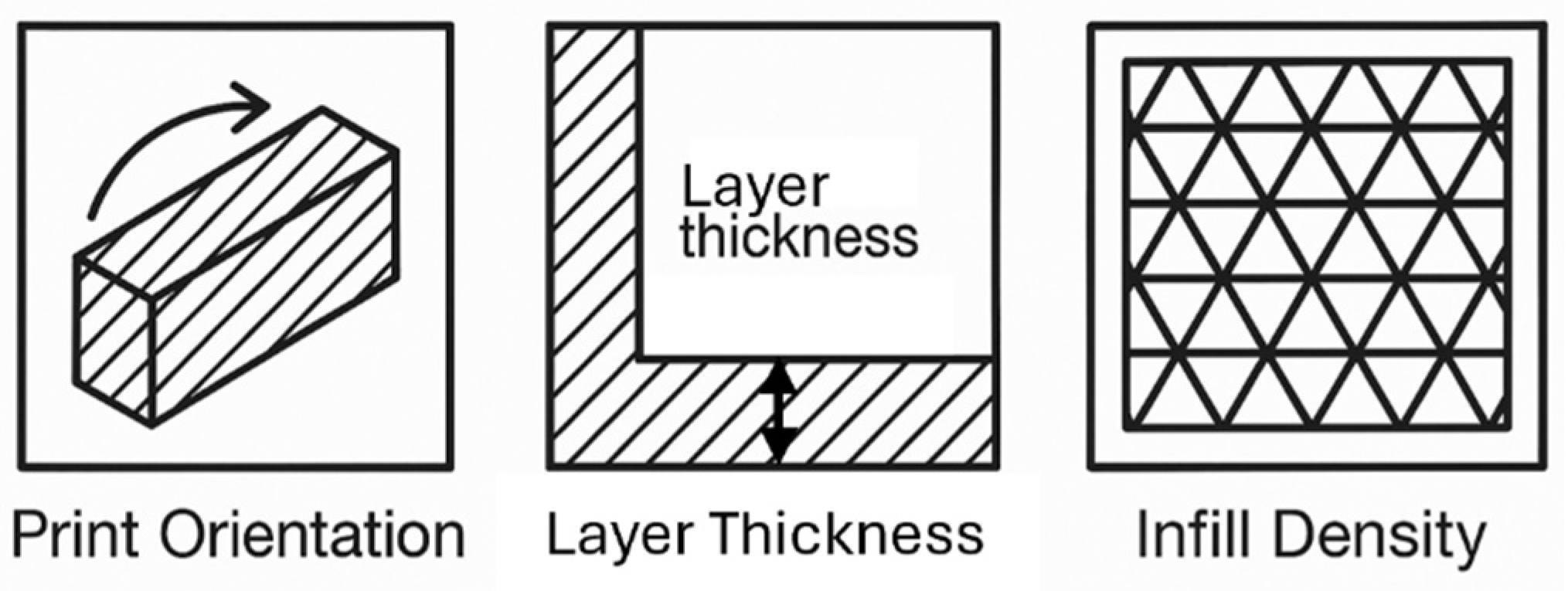
Figure 2.
General outline of the methodology, including data acquisition, processing, and analysis.
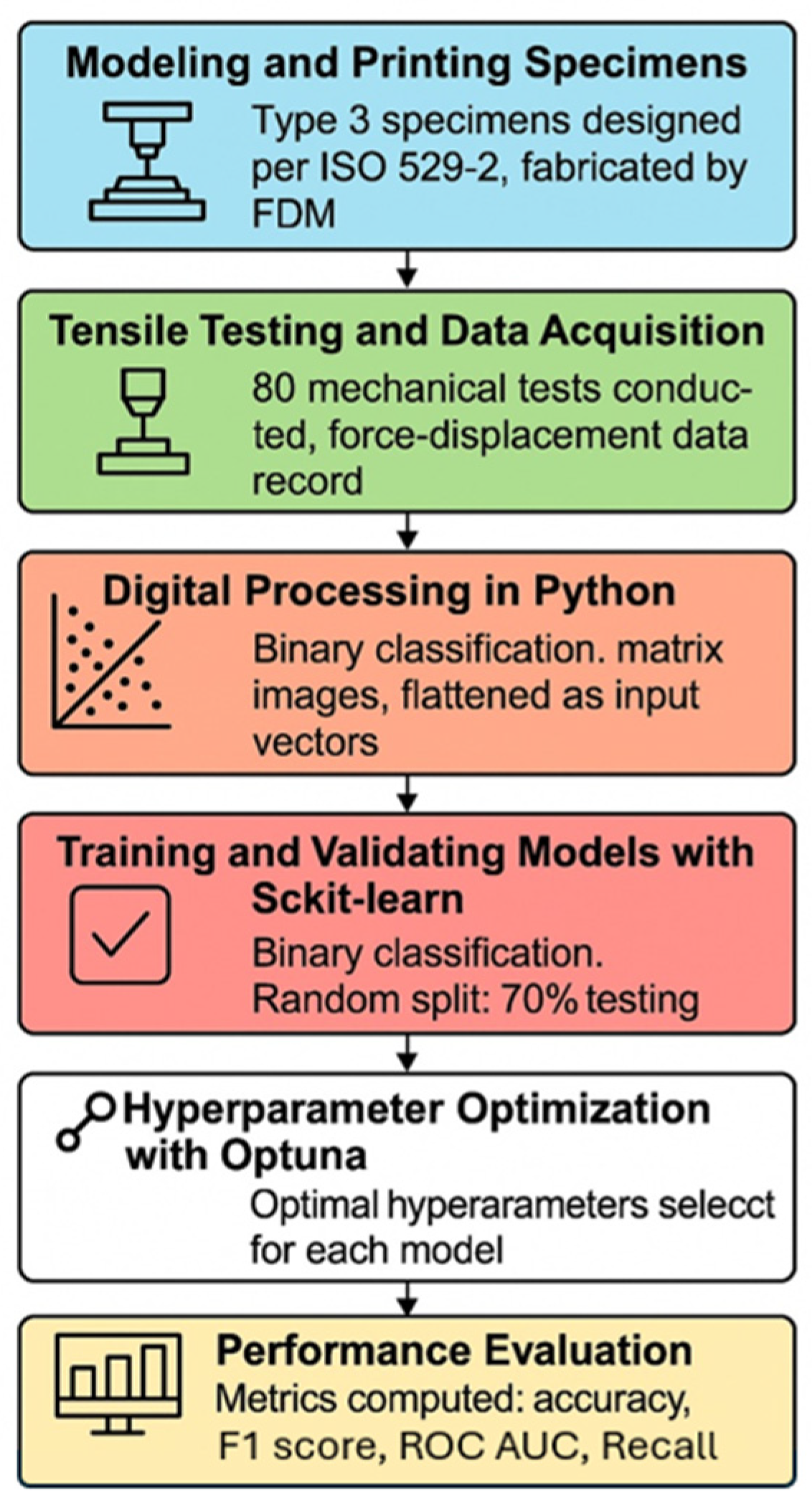
Figure 3.
(a) A Tensile test specimen according to ISO 527-2 Type 1A; (b) Universal Testing Machine Shimadzu.
Figure 3.
(a) A Tensile test specimen according to ISO 527-2 Type 1A; (b) Universal Testing Machine Shimadzu.
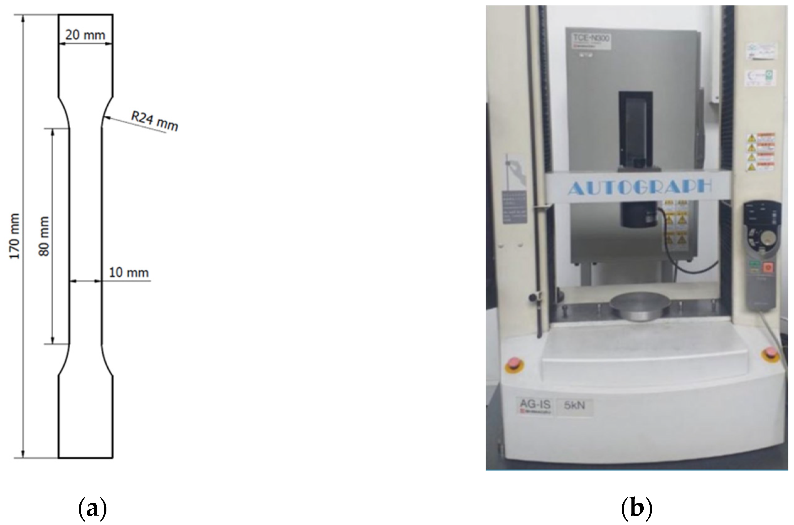
Figure 4.
(a) Force-displacement graph before and after treatment with moving average; (b) Stress-strain graph before and after treatment with moving average.
Figure 4.
(a) Force-displacement graph before and after treatment with moving average; (b) Stress-strain graph before and after treatment with moving average.
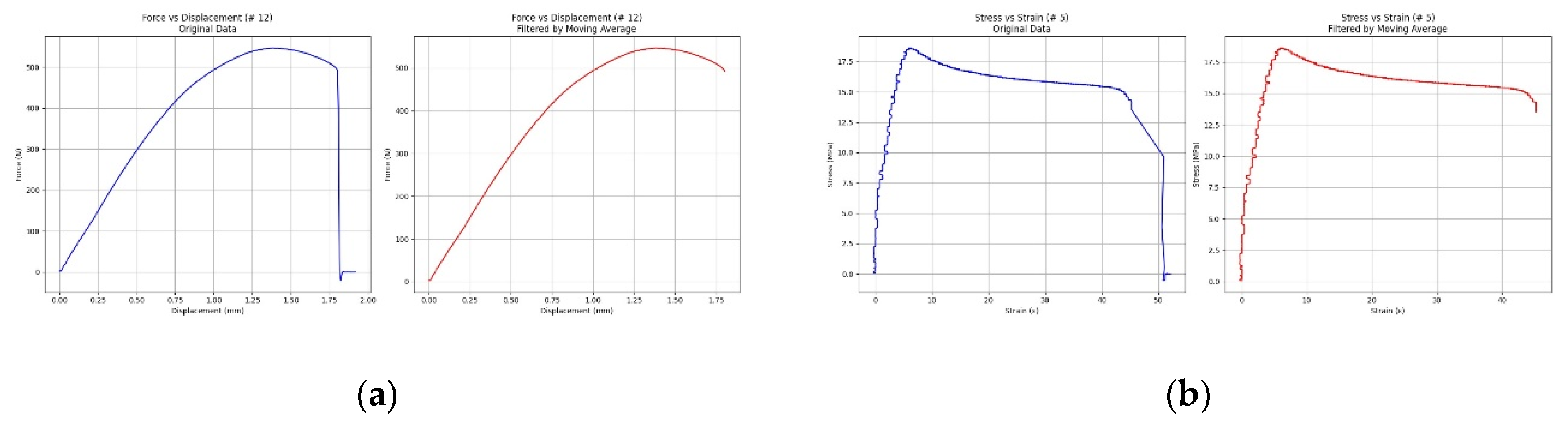
Figure 5.
Box plots showing the results for Precision, F1 score, Recall, and ROC AUC for each model.
Figure 5.
Box plots showing the results for Precision, F1 score, Recall, and ROC AUC for each model.
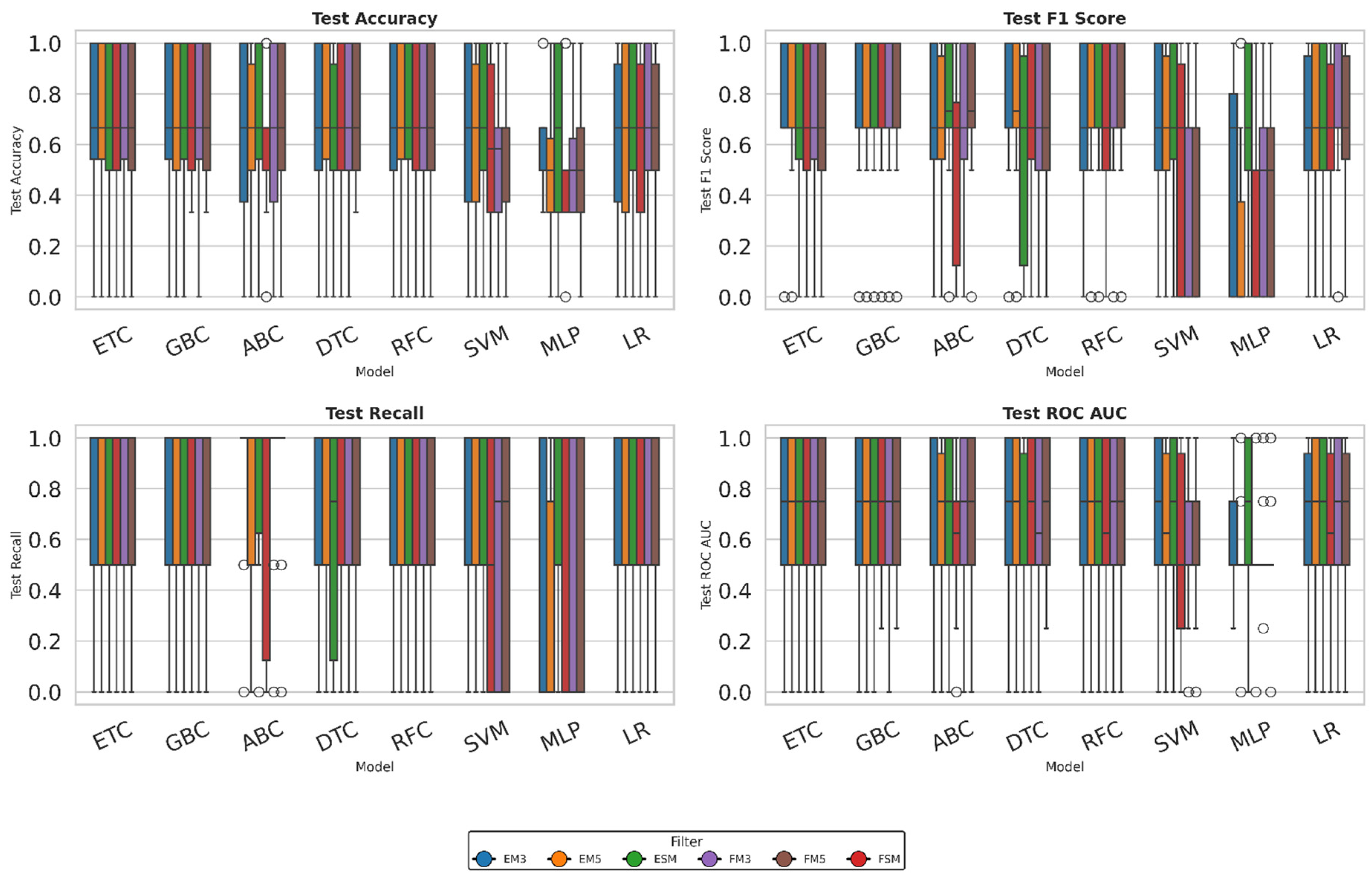
Figure 6.
Heatmaps of model performance across metrics and filter configurations.
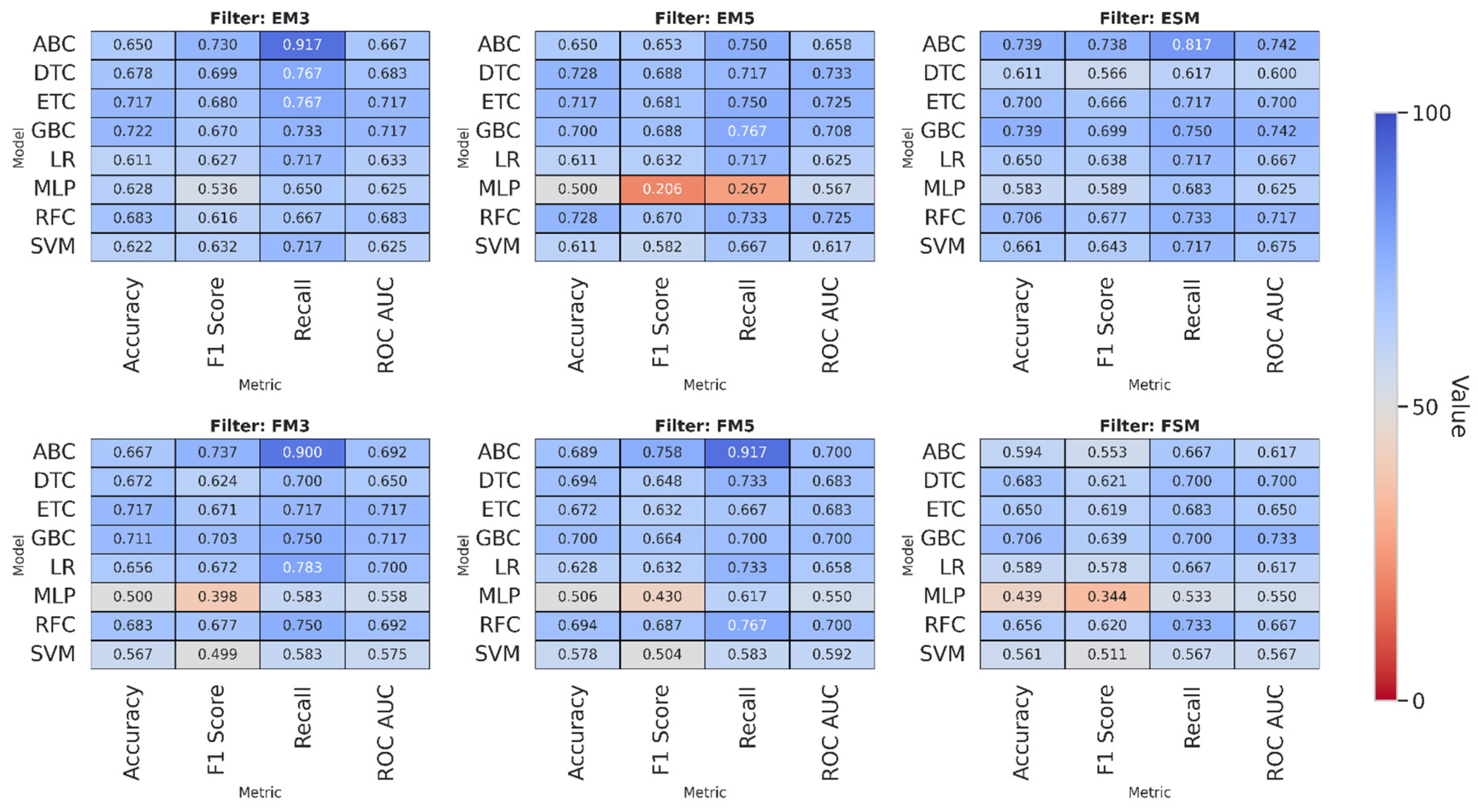
Figure 7.
Box plots showing the results for Precision, F1 score, Recall, and ROC AUC for each model.
Figure 7.
Box plots showing the results for Precision, F1 score, Recall, and ROC AUC for each model.
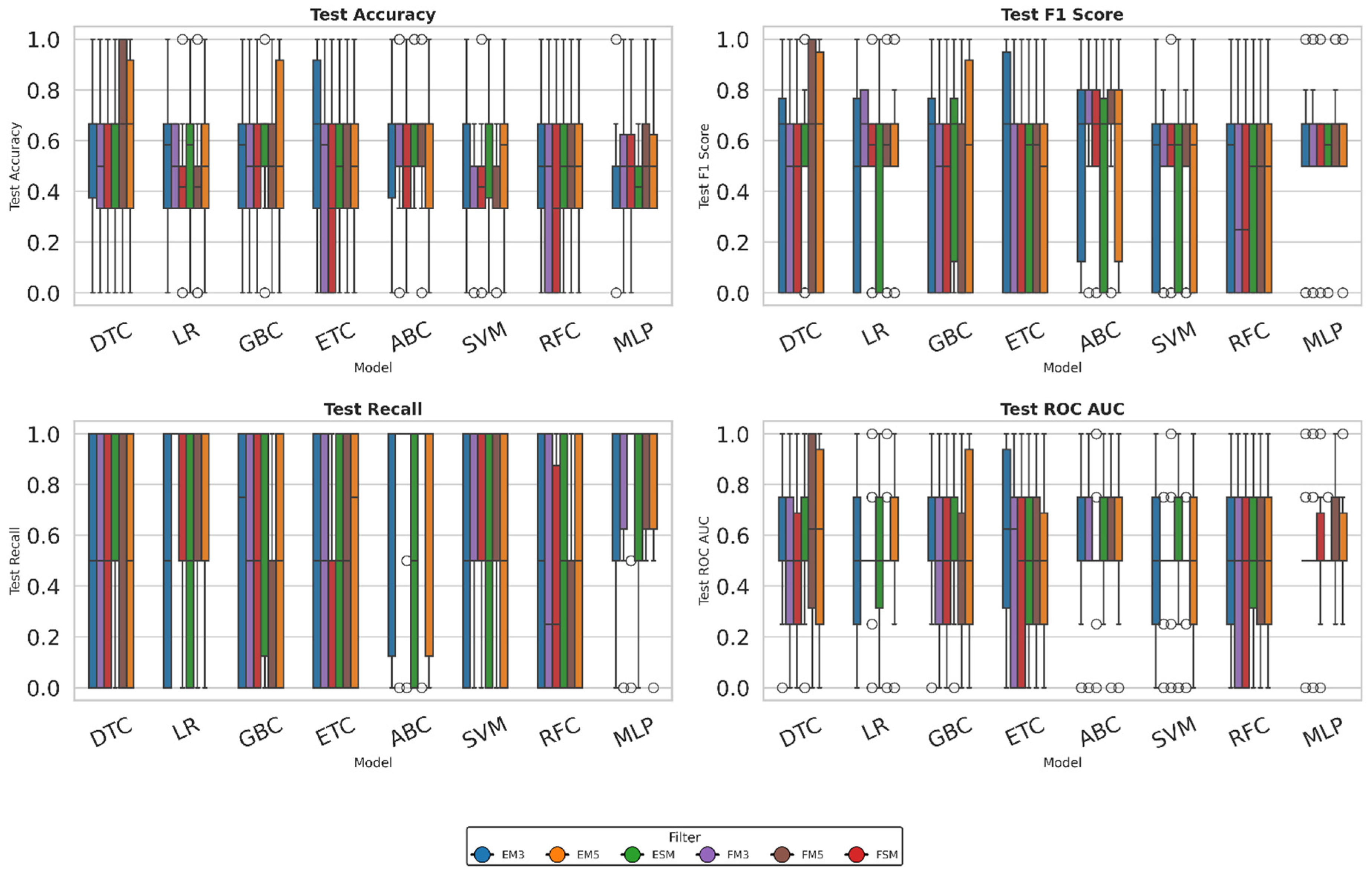
Figure 8.
Heatmaps of model performance across metrics and filter configurations.
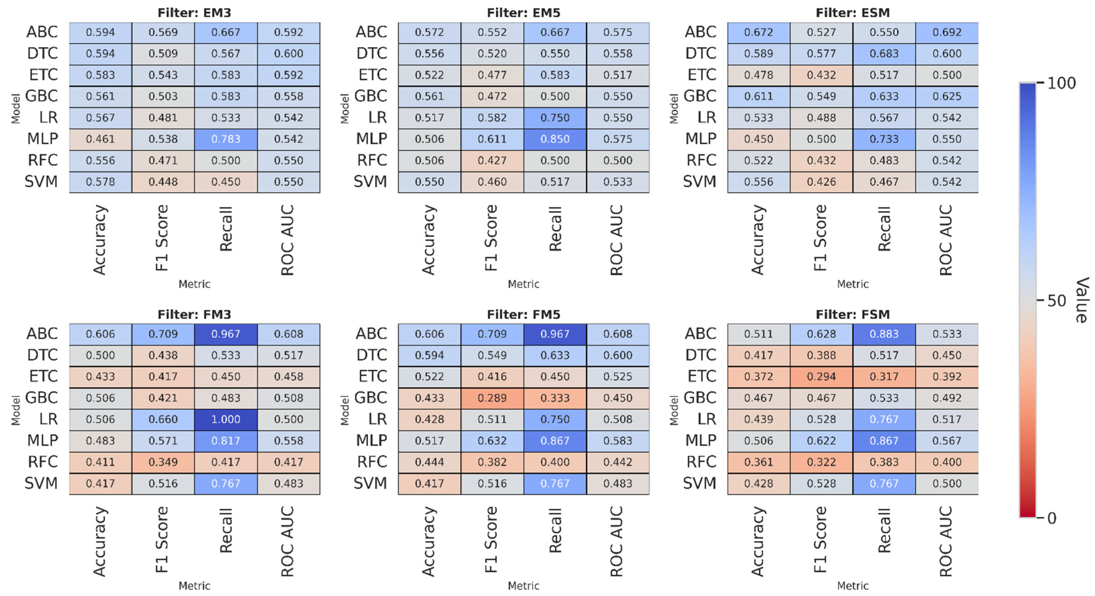
Figure 9.
Box plots showing the results for Precision, F1 score, Recall, and ROC AUC for each model.
Figure 9.
Box plots showing the results for Precision, F1 score, Recall, and ROC AUC for each model.
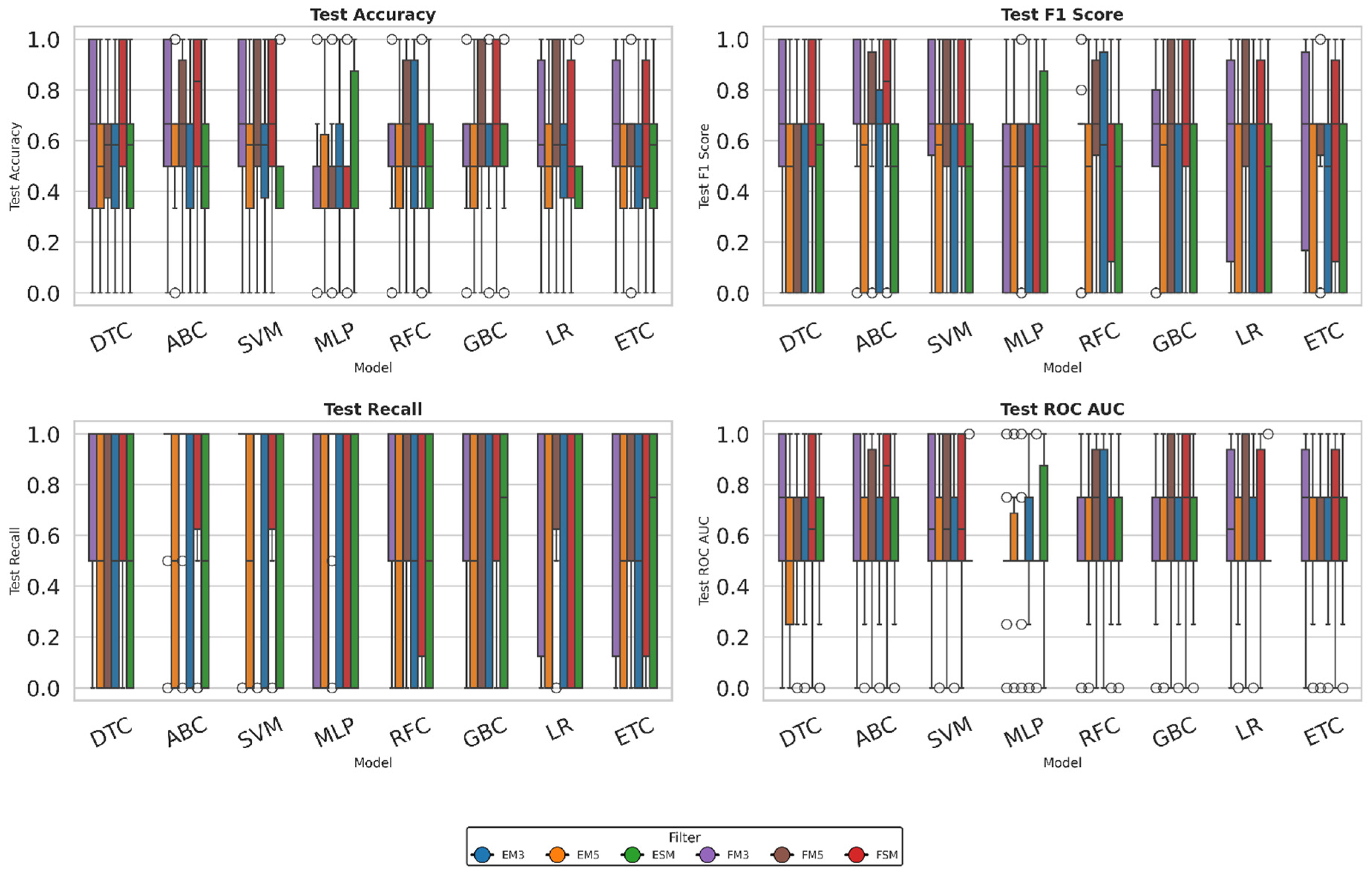
Figure 10.
Heatmaps of model performance across metrics and filter configurations.
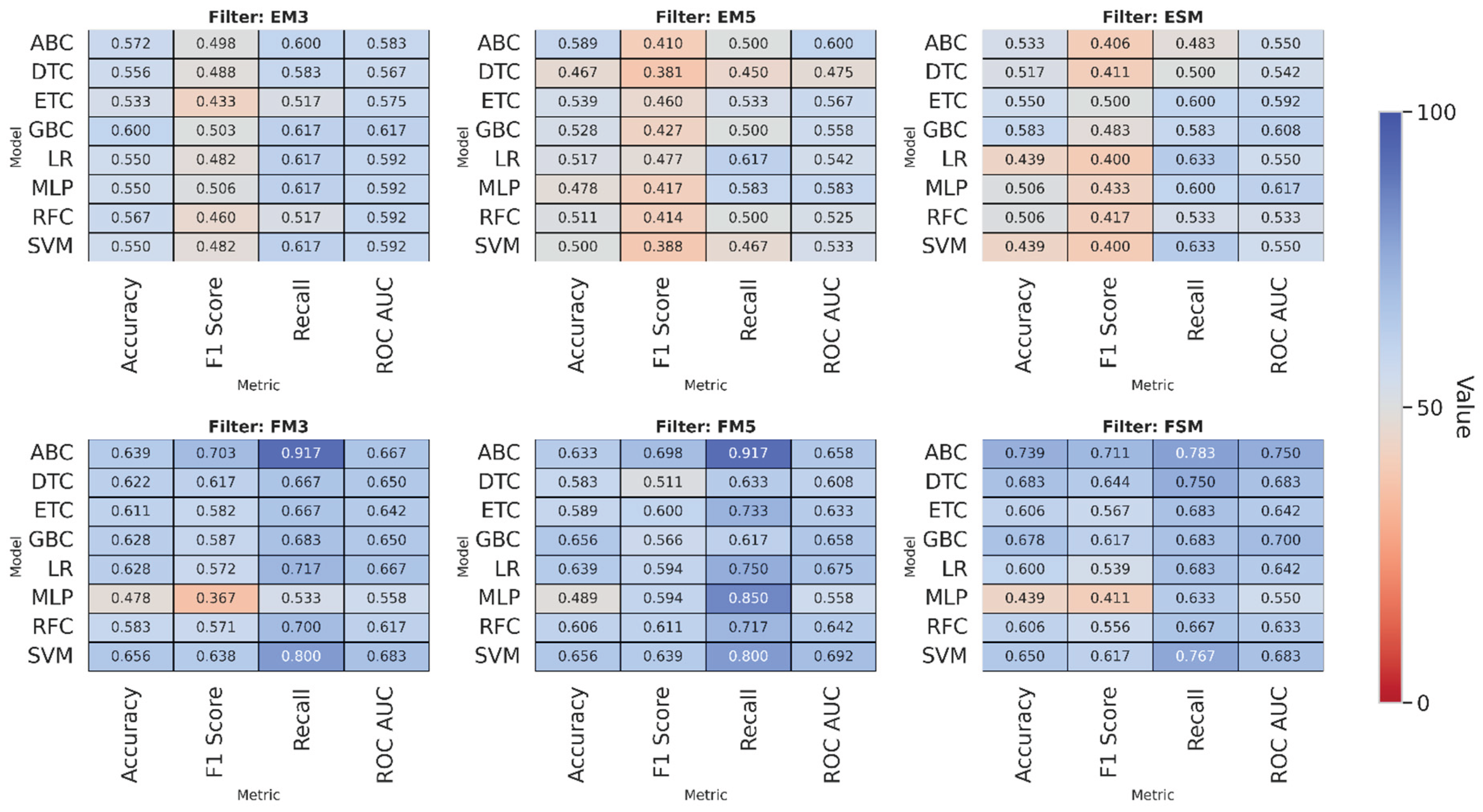

Table 1.
Hyperparameters and ranges or values for hyperparameter optimization.
| Models | Hyperparameters | ranges/values | References |
| DecisionTreeClassifier | Criterion | Gini, entropy | [29,30,31,32] |
| Max_depth | None, 5, 10, 20 | ||
| Min_samples_split | 2, 5, 10 | ||
| Min_samples_leaf | 1, 2, 4 | ||
| AdaBoostClassifier | N_estimators | 50, 100, 200 | |
| Learning_rate | 0.01, 0.1, 1.0 | ||
| Support Vector Machines | C | 0.1, 1, 10 | |
| kernel | Linear, rbf | ||
| gamma | Scale, auto | ||
| Multilayer Perceptron | Hidden_layer | 50 - 150 | |
| N_layers | 1 - 3 | ||
| activation | Identity, logistic, tanh, relu | ||
| solver | Adam, sgd | ||
| alpha | 1e-5 – 1e-1 | ||
| Learning_rate | Constant, invscaling, adaptive | ||
| RandomForestClassifier | N_estimators | 100, 200 | |
| Max_depth | None, 10, 20 | ||
| Min_samples_split | 2, 5 | ||
| Min_samples_leaf | 1, 2 | ||
| bootstrap | True, false | ||
| GradientBoostingClassifier | N_estimators | 50 - 200 | |
| Learning_rate | 0.01 - 0.2 | ||
| Max_depth | 3 - 10 | ||
| Min_samples_split | 2 - 10 | ||
| Min_samples_leaf | 1 - 5 | ||
| LogisticRegression | penalty | L1, l2, elasticnet, none | |
| solver | Liblinear, lbfgs, saga, newton-cg | ||
| C | 1e-3 - 10 | ||
| ExtraTreesClassifier | N_estimators | 100, 200 | |
| Max_depth | None, 10, 20 | ||
| Min_samples_split | 2, 5 | ||
| Min_samples_leaf | 1, 2 | ||
| bootstrap | True, false |
Table 2.
Test accuracy by model with minimum, maximum, mean, and standard deviation values.
| Model | Filter | Min. | Max. | Mean | Std. Dev. |
| AdaBoost | EM3 | 0 | 1 | 0.650 | 0.291 |
| EM5 | 0 | 1 | 0.650 | 0.264 | |
| ESM | 0 | 1 | 0.739 | 0.286 | |
| FM3 | 0 | 1 | 0.667 | 0.297 | |
| FM5 | 0 | 1 | 0.689 | 0.296 | |
| FSM | 0 | 1 | 0.594 | 0.289 | |
| ExtraTrees | EM3 | 0 | 1 | 0.717 | 0.240 |
| EM5 | 0 | 1 | 0.717 | 0.259 | |
| ESM | 0 | 1 | 0.700 | 0.271 | |
| FM3 | 0 | 1 | 0.717 | 0.304 | |
| FM5 | 0 | 1 | 0.672 | 0.332 | |
| FSM | 0 | 1 | 0.650 | 0.320 | |
| GradientBoosting | EM3 | 0 | 1 | 0.722 | 0.271 |
| EM5 | 0 | 1 | 0.700 | 0.275 | |
| ESM | 0 | 1 | 0.739 | 0.269 | |
| FM3 | 0 | 1 | 0.711 | 0.266 | |
| FM5 | 0.333 | 1 | 0.700 | 0.245 | |
| FSM | 0.333 | 1 | 0.706 | 0.238 | |
| LogisticRegression |
EM3 | 0 | 1 | 0.611 | 0.311 |
| EM5 | 0 | 1 | 0.611 | 0.323 | |
| ESM | 0 | 1 | 0.650 | 0.291 | |
| FM3 | 0 | 1 | 0.656 | 0.303 | |
| FM5 | 0 | 1 | 0.628 | 0.289 | |
| FSM | 0 | 1 | 0.589 | 0.318 | |
| MLP |
EM3 | 0.333 | 1 | 0.628 | 0.242 |
| EM5 | 0 | 1 | 0.500 | 0.223 | |
| ESM | 0 | 1 | 0.583 | 0.352 | |
| FM3 | 0.333 | 1 | 0.500 | 0.210 | |
| FM5 | 0 | 1 | 0.506 | 0.229 | |
| FSM | 0 | 1 | 0.439 | 0.242 | |
| RandomForest |
EM3 | 0 | 1 | 0.683 | 0.271 |
| EM5 | 0 | 1 | 0.728 | 0.264 | |
| ESM | 0 | 1 | 0.706 | 0.283 | |
| FM3 | 0 | 1 | 0.683 | 0.275 | |
| FM5 | 0 | 1 | 0.694 | 0.294 | |
| FSM | 0 | 1 | 0.656 | 0.277 | |
| SVM |
EM3 | 0 | 1 | 0.622 | 0.318 |
| EM5 | 0 | 1 | 0.611 | 0.311 | |
| ESM | 0 | 1 | 0.661 | 0.285 | |
| FM3 | 0 | 1 | 0.567 | 0.296 | |
| FM5 | 0 | 1 | 0.578 | 0.293 | |
| FSM | 0 | 1 | 0.561 | 0.338 | |
| DecisionTree |
EM3 | 0 | 1 | 0.678 | 0.350 |
| EM5 | 0 | 1 | 0.728 | 0.308 | |
| ESM | 0 | 1 | 0.611 | 0.307 | |
| FM3 | 0 | 1 | 0.672 | 0.268 | |
| FM5 | 0.333 | 1 | 0.694 | 0.252 | |
| FSM | 0 | 1 | 0.683 | 0.271 |
Table 3.
Test f1 by model with minimum, maximum, mean, and standard deviation values.
| Model | Filter | Min. | Max. | Mean | Std. Dev. |
| AdaBoost | EM3 | 0 | 1 | 0.730 | 0.241 |
| EM5 | 0 | 1 | 0.653 | 0.311 | |
| ESM | 0 | 1 | 0.738 | 0.314 | |
| FM3 | 0 | 1 | 0.737 | 0.246 | |
| FM5 | 0 | 1 | 0.758 | 0.246 | |
| FSM | 0 | 1 | 0.553 | 0.368 | |
| ExtraTrees | EM3 | 0 | 1 | 0.680 | 0.341 |
| EM5 | 0 | 1 | 0.681 | 0.347 | |
| ESM | 0 | 1 | 0.666 | 0.350 | |
| FM3 | 0 | 1 | 0.671 | 0.380 | |
| FM5 | 0 | 1 | 0.632 | 0.394 | |
| FSM | 0 | 1 | 0.619 | 0.385 | |
| GradientBoosting | EM3 | 0 | 1 | 0.670 | 0.374 |
| EM5 | 0 | 1 | 0.688 | 0.326 | |
| ESM | 0 | 1 | 0.699 | 0.356 | |
| FM3 | 0 | 1 | 0.703 | 0.323 | |
| FM5 | 0 | 1 | 0.664 | 0.344 | |
| FSM | 0 | 1 | 0.639 | 0.361 | |
| LogisticRegression |
EM3 | 0 | 1 | 0.627 | 0.332 |
| EM5 | 0 | 1 | 0.632 | 0.340 | |
| ESM | 0 | 1 | 0.638 | 0.339 | |
| FM3 | 0 | 1 | 0.672 | 0.320 | |
| FM5 | 0 | 1 | 0.632 | 0.331 | |
| FSM | 0 | 1 | 0.578 | 0.365 | |
| MLP |
EM3 | 0 | 1 | 0.536 | 0.391 |
| EM5 | 0 | 1 | 0.206 | 0.360 | |
| ESM | 0 | 1 | 0.589 | 0.373 | |
| FM3 | 0 | 1 | 0.398 | 0.360 | |
| FM5 | 0 | 1 | 0.430 | 0.361 | |
| FSM | 0 | 1 | 0.344 | 0.363 | |
| RandomForest |
EM3 | 0 | 1 | 0.616 | 0.381 |
| EM5 | 0 | 1 | 0.670 | 0.374 | |
| ESM | 0 | 1 | 0.677 | 0.347 | |
| FM3 | 0 | 1 | 0.677 | 0.321 | |
| FM5 | 0 | 1 | 0.687 | 0.354 | |
| FSM | 0 | 1 | 0.620 | 0.360 | |
| SVM |
EM3 | 0 | 1 | 0.632 | 0.340 |
| EM5 | 0 | 1 | 0.582 | 0.367 | |
| ESM | 0 | 1 | 0.643 | 0.338 | |
| FM3 | 0 | 1 | 0.499 | 0.388 | |
| FM5 | 0 | 1 | 0.504 | 0.389 | |
| FSM | 0 | 1 | 0.511 | 0.403 | |
| DecisionTree |
EM3 | 0 | 1 | 0.699 | 0.356 |
| EM5 | 0 | 1 | 0.688 | 0.383 | |
| ESM | 0 | 1 | 0.566 | 0.382 | |
| FM3 | 0 | 1 | 0.624 | 0.361 | |
| FM5 | 0 | 1 | 0.648 | 0.347 | |
| FSM | 0 | 1 | 0.621 | 0.381 |
Table 4.
Test recall by model with minimum, maximum, mean, and standard deviation values.
| Model | Filter | Min. | Max. | Mean | Std. Dev. |
| AdaBoost | EM3 | 0 | 1 | 0.917 | 0.231 |
| EM5 | 0 | 1 | 0.750 | 0.366 | |
| ESM | 0 | 1 | 0.817 | 0.334 | |
| FM3 | 0 | 1 | 0.900 | 0.242 | |
| FM5 | 0 | 1 | 0.917 | 0.231 | |
| FSM | 0 | 1 | 0.667 | 0.442 | |
| ExtraTrees | EM3 | 0 | 1 | 0.767 | 0.388 |
| EM5 | 0 | 1 | 0.750 | 0.388 | |
| ESM | 0 | 1 | 0.717 | 0.387 | |
| FM3 | 0 | 1 | 0.717 | 0.409 | |
| FM5 | 0 | 1 | 0.667 | 0.422 | |
| FSM | 0 | 1 | 0.683 | 0.425 | |
| GradientBoosting | EM3 | 0 | 1 | 0.733 | 0.410 |
| EM5 | 0 | 1 | 0.767 | 0.365 | |
| ESM | 0 | 1 | 0.750 | 0.388 | |
| FM3 | 0 | 1 | 0.750 | 0.366 | |
| FM5 | 0 | 1 | 0.700 | 0.385 | |
| FSM | 0 | 1 | 0.700 | 0.407 | |
| LogisticRegression |
EM3 | 0 | 1 | 0.717 | 0.387 |
| EM5 | 0 | 1 | 0.717 | 0.387 | |
| ESM | 0 | 1 | 0.717 | 0.387 | |
| FM3 | 0 | 1 | 0.783 | 0.364 | |
| FM5 | 0 | 1 | 0.733 | 0.388 | |
| FSM | 0 | 1 | 0.667 | 0.422 | |
| MLP |
EM3 | 0 | 1 | 0.650 | 0.458 |
| EM5 | 0 | 1 | 0.267 | 0.450 | |
| ESM | 0 | 1 | 0.683 | 0.425 | |
| FM3 | 0 | 1 | 0.583 | 0.493 | |
| FM5 | 0 | 1 | 0.617 | 0.486 | |
| FSM | 0 | 1 | 0.533 | 0.507 | |
| RandomForest |
EM3 | 0 | 1 | 0.667 | 0.422 |
| EM5 | 0 | 1 | 0.733 | 0.410 | |
| ESM | 0 | 1 | 0.733 | 0.388 | |
| FM3 | 0 | 1 | 0.750 | 0.366 | |
| FM5 | 0 | 1 | 0.767 | 0.388 | |
| FSM | 0 | 1 | 0.733 | 0.410 | |
| SVM |
EM3 | 0 | 1 | 0.717 | 0.387 |
| EM5 | 0 | 1 | 0.667 | 0.422 | |
| ESM | 0 | 1 | 0.717 | 0.387 | |
| FM3 | 0 | 1 | 0.583 | 0.456 | |
| FM5 | 0 | 1 | 0.583 | 0.456 | |
| FSM | 0 | 1 | 0.567 | 0.450 | |
| DecisionTree |
EM3 | 0 | 1 | 0.767 | 0.388 |
| EM5 | 0 | 1 | 0.717 | 0.409 | |
| ESM | 0 | 1 | 0.617 | 0.429 | |
| FM3 | 0 | 1 | 0.700 | 0.407 | |
| FM5 | 0 | 1 | 0.733 | 0.388 | |
| FSM | 0 | 1 | 0.700 | 0.428 |
Table 5.
Test ROC AUC by model with minimum, maximum, mean, and standard deviation values.
| Model | Filter | Min. | Max. | Mean | Std. Dev. |
| AdaBoost | EM3 | 0 | 1 | 0.667 | 0.281 |
| EM5 | 0 | 1 | 0.658 | 0.275 | |
| ESM | 0 | 1 | 0.742 | 0.297 | |
| FM3 | 0 | 1 | 0.692 | 0.284 | |
| FM5 | 0 | 1 | 0.700 | 0.289 | |
| FSM | 0 | 1 | 0.617 | 0.292 | |
| ExtraTrees | EM3 | 0 | 1 | 0.717 | 0.252 |
| EM5 | 0 | 1 | 0.725 | 0.265 | |
| ESM | 0 | 1 | 0.700 | 0.282 | |
| FM3 | 0 | 1 | 0.717 | 0.313 | |
| FM5 | 0 | 1 | 0.683 | 0.334 | |
| FSM | 0 | 1 | 0.650 | 0.326 | |
| GradientBoosting | EM3 | 0 | 1 | 0.717 | 0.284 |
| EM5 | 0 | 1 | 0.708 | 0.279 | |
| ESM | 0 | 1 | 0.742 | 0.275 | |
| FM3 | 0 | 1 | 0.717 | 0.284 | |
| FM5 | 0.25 | 1 | 0.700 | 0.274 | |
| FSM | 0.25 | 1 | 0.733 | 0.236 | |
| LogisticRegression |
EM3 | 0 | 1 | 0.633 | 0.320 |
| EM5 | 0 | 1 | 0.625 | 0.333 | |
| ESM | 0 | 1 | 0.667 | 0.296 | |
| FM3 | 0 | 1 | 0.700 | 0.289 | |
| FM5 | 0 | 1 | 0.658 | 0.290 | |
| FSM | 0 | 1 | 0.617 | 0.320 | |
| MLP |
EM3 | 0.25 | 1 | 0.625 | 0.234 |
| EM5 | 0 | 1 | 0.567 | 0.196 | |
| ESM | 0 | 1 | 0.625 | 0.346 | |
| FM3 | 0.25 | 1 | 0.558 | 0.170 | |
| FM5 | 0 | 1 | 0.550 | 0.190 | |
| FSM | 0 | 1 | 0.550 | 0.201 | |
| RandomForest |
EM3 | 0 | 1 | 0.683 | 0.286 |
| EM5 | 0 | 1 | 0.725 | 0.273 | |
| ESM | 0 | 1 | 0.717 | 0.292 | |
| FM3 | 0 | 1 | 0.692 | 0.291 | |
| FM5 | 0 | 1 | 0.700 | 0.304 | |
| FSM | 0 | 1 | 0.667 | 0.273 | |
| SVM |
EM3 | 0 | 1 | 0.625 | 0.333 |
| EM5 | 0 | 1 | 0.617 | 0.320 | |
| ESM | 0 | 1 | 0.675 | 0.295 | |
| FM3 | 0 | 1 | 0.575 | 0.309 | |
| FM5 | 0 | 1 | 0.592 | 0.304 | |
| FSM | 0 | 1 | 0.567 | 0.347 | |
| DecisionTree |
EM3 | 0 | 1 | 0.683 | 0.359 |
| EM5 | 0 | 1 | 0.733 | 0.314 | |
| ESM | 0 | 1 | 0.600 | 0.326 | |
| FM3 | 0 | 1 | 0.650 | 0.291 | |
| FM5 | 0.25 | 1 | 0.683 | 0.270 | |
| FSM | 0 | 1 | 0.700 | 0.274 |
Table 6.
Test accuracy by model with minimum, maximum, mean, and standard deviation values.
| Model | Filter | Min. | Max. | Mean | Std. Dev. |
| AdaBoost | EM3 | 0 | 1 | 0.594 | 0.302 |
| EM5 | 0 | 1 | 0.572 | 0.296 | |
| ESM | 0.333 | 1 | 0.672 | 0.212 | |
| FM3 | 0 | 1 | 0.606 | 0.253 | |
| FM5 | 0 | 1 | 0.606 | 0.253 | |
| FSM | 0 | 1 | 0.511 | 0.262 | |
| ExtraTrees | EM3 | 0 | 1 | 0.583 | 0.333 |
| EM5 | 0 | 1 | 0.522 | 0.289 | |
| ESM | 0 | 1 | 0.478 | 0.330 | |
| FM3 | 0 | 1 | 0.433 | 0.370 | |
| FM5 | 0 | 1 | 0.522 | 0.306 | |
| FSM | 0 | 1 | 0.372 | 0.315 | |
| GradientBoosting | EM3 | 0 | 1 | 0.561 | 0.298 |
| EM5 | 0 | 1 | 0.561 | 0.335 | |
| ESM | 0 | 1 | 0.611 | 0.281 | |
| FM3 | 0 | 1 | 0.506 | 0.317 | |
| FM5 | 0 | 1 | 0.433 | 0.282 | |
| FSM | 0 | 1 | 0.467 | 0.340 | |
| LogisticRegression |
EM3 | 0 | 1 | 0.567 | 0.286 |
| EM5 | 0 | 1 | 0.517 | 0.275 | |
| ESM | 0 | 1 | 0.533 | 0.260 | |
| FM3 | 0.333 | 0.667 | 0.506 | 0.142 | |
| FM5 | 0 | 1 | 0.428 | 0.213 | |
| FSM | 0 | 1 | 0.439 | 0.198 | |
| MLP |
EM3 | 0 | 1 | 0.461 | 0.184 |
| EM5 | 0.333 | 1 | 0.506 | 0.208 | |
| ESM | 0.333 | 0.667 | 0.450 | 0.132 | |
| FM3 | 0 | 1 | 0.483 | 0.207 | |
| FM5 | 0.333 | 1 | 0.517 | 0.187 | |
| FSM | 0 | 1 | 0.506 | 0.242 | |
| RandomForest |
EM3 | 0 | 1 | 0.556 | 0.288 |
| EM5 | 0 | 1 | 0.506 | 0.246 | |
| ESM | 0 | 1 | 0.522 | 0.330 | |
| FM3 | 0 | 1 | 0.411 | 0.318 | |
| FM5 | 0 | 1 | 0.444 | 0.304 | |
| FSM | 0 | 1 | 0.361 | 0.300 | |
| SVM |
EM3 | 0 | 1 | 0.578 | 0.269 |
| EM5 | 0 | 1 | 0.550 | 0.288 | |
| ESM | 0 | 1 | 0.556 | 0.241 | |
| FM3 | 0 | 0.667 | 0.417 | 0.168 | |
| FM5 | 0 | 0.667 | 0.417 | 0.168 | |
| FSM | 0 | 1 | 0.428 | 0.213 | |
| DecisionTree |
EM3 | 0 | 1 | 0.594 | 0.276 |
| EM5 | 0 | 1 | 0.556 | 0.362 | |
| ESM | 0 | 1 | 0.589 | 0.279 | |
| FM3 | 0 | 1 | 0.500 | 0.294 | |
| FM5 | 0 | 1 | 0.594 | 0.363 | |
| FSM | 0 | 1 | 0.417 | 0.279 |
Table 7.
Test F1 by model with minimum, maximum, mean, and standard deviation values.
| Model | Filter | Min. | Max. | Mean | Std. Dev. |
| AdaBoost | EM3 | 0 | 1 | 0.569 | 0.379 |
| EM5 | 0 | 1 | 0.552 | 0.370 | |
| ESM | 0 | 1 | 0.527 | 0.401 | |
| FM3 | 0 | 1 | 0.709 | 0.216 | |
| FM5 | 0 | 1 | 0.709 | 0.216 | |
| FSM | 0 | 1 | 0.628 | 0.241 | |
| ExtraTrees | EM3 | 0 | 1 | 0.543 | 0.395 |
| EM5 | 0 | 1 | 0.477 | 0.382 | |
| ESM | 0 | 1 | 0.432 | 0.382 | |
| FM3 | 0 | 1 | 0.417 | 0.388 | |
| FM5 | 0 | 1 | 0.416 | 0.390 | |
| FSM | 0 | 1 | 0.294 | 0.357 | |
| GradientBoosting | EM3 | 0 | 1 | 0.503 | 0.391 |
| EM5 | 0 | 1 | 0.472 | 0.422 | |
| ESM | 0 | 1 | 0.549 | 0.374 | |
| FM3 | 0 | 1 | 0.421 | 0.399 | |
| FM5 | 0 | 1 | 0.289 | 0.353 | |
| FSM | 0 | 1 | 0.467 | 0.370 | |
| LogisticRegression |
EM3 | 0 | 1 | 0.481 | 0.385 |
| EM5 | 0 | 1 | 0.582 | 0.278 | |
| ESM | 0 | 1 | 0.488 | 0.346 | |
| FM3 | 0.5 | 0.8 | 0.660 | 0.128 | |
| FM5 | 0 | 1 | 0.511 | 0.255 | |
| FSM | 0 | 1 | 0.528 | 0.236 | |
| MLP |
EM3 | 0 | 1 | 0.538 | 0.241 |
| EM5 | 0 | 1 | 0.611 | 0.187 | |
| ESM | 0 | 0.667 | 0.500 | 0.240 | |
| FM3 | 0 | 1 | 0.571 | 0.233 | |
| FM5 | 0.5 | 1 | 0.632 | 0.133 | |
| FSM | 0 | 1 | 0.622 | 0.200 | |
| RandomForest |
EM3 | 0 | 1 | 0.471 | 0.396 |
| EM5 | 0 | 1 | 0.427 | 0.356 | |
| ESM | 0 | 1 | 0.432 | 0.411 | |
| FM3 | 0 | 1 | 0.349 | 0.368 | |
| FM5 | 0 | 1 | 0.382 | 0.357 | |
| FSM | 0 | 1 | 0.322 | 0.339 | |
| SVM |
EM3 | 0 | 1 | 0.448 | 0.397 |
| EM5 | 0 | 1 | 0.460 | 0.385 | |
| ESM | 0 | 1 | 0.426 | 0.373 | |
| FM3 | 0 | 0.8 | 0.516 | 0.223 | |
| FM5 | 0 | 0.8 | 0.516 | 0.223 | |
| FSM | 0 | 1 | 0.528 | 0.236 | |
| DecisionTree |
EM3 | 0 | 1 | 0.509 | 0.392 |
| EM5 | 0 | 1 | 0.520 | 0.422 | |
| ESM | 0 | 1 | 0.577 | 0.335 | |
| FM3 | 0 | 1 | 0.438 | 0.369 | |
| FM5 | 0 | 1 | 0.549 | 0.424 | |
| FSM | 0 | 1 | 0.388 | 0.344 |
Table 8.
Test Recall by model with minimum, maximum, mean, and standard deviation values.
| Model | Filter | Min. | Max. | Mean | Std. Dev. |
| AdaBoost | EM3 | 0 | 1 | 0.667 | 0.442 |
| EM5 | 0 | 1 | 0.667 | 0.442 | |
| ESM | 0 | 1 | 0.550 | 0.442 | |
| FM3 | 0 | 1 | 0.967 | 0.183 | |
| FM5 | 0 | 1 | 0.967 | 0.183 | |
| FSM | 0 | 1 | 0.883 | 0.284 | |
| ExtraTrees | EM3 | 0 | 1 | 0.583 | 0.437 |
| EM5 | 0 | 1 | 0.583 | 0.456 | |
| ESM | 0 | 1 | 0.517 | 0.464 | |
| FM3 | 0 | 1 | 0.450 | 0.442 | |
| FM5 | 0 | 1 | 0.450 | 0.442 | |
| FSM | 0 | 1 | 0.317 | 0.404 | |
| GradientBoosting | EM3 | 0 | 1 | 0.583 | 0.456 |
| EM5 | 0 | 1 | 0.500 | 0.455 | |
| ESM | 0 | 1 | 0.633 | 0.434 | |
| FM3 | 0 | 1 | 0.483 | 0.464 | |
| FM5 | 0 | 1 | 0.333 | 0.422 | |
| FSM | 0 | 1 | 0.533 | 0.434 | |
| LogisticRegression |
EM3 | 0 | 1 | 0.533 | 0.434 |
| EM5 | 0 | 1 | 0.750 | 0.366 | |
| ESM | 0 | 1 | 0.567 | 0.430 | |
| FM3 | 1 | 1 | 1.000 | 0.000 | |
| FM5 | 0 | 1 | 0.750 | 0.388 | |
| FSM | 0 | 1 | 0.767 | 0.365 | |
| MLP |
EM3 | 0 | 1 | 0.783 | 0.364 |
| EM5 | 0 | 1 | 0.850 | 0.267 | |
| ESM | 0 | 1 | 0.733 | 0.388 | |
| FM3 | 0 | 1 | 0.817 | 0.334 | |
| FM5 | 0.5 | 1 | 0.867 | 0.225 | |
| FSM | 0 | 1 | 0.867 | 0.260 | |
| RandomForest |
EM3 | 0 | 1 | 0.500 | 0.435 |
| EM5 | 0 | 1 | 0.500 | 0.435 | |
| ESM | 0 | 1 | 0.483 | 0.464 | |
| FM3 | 0 | 1 | 0.417 | 0.456 | |
| FM5 | 0 | 1 | 0.400 | 0.403 | |
| FSM | 0 | 1 | 0.383 | 0.429 | |
| SVM |
EM3 | 0 | 1 | 0.450 | 0.422 |
| EM5 | 0 | 1 | 0.517 | 0.445 | |
| ESM | 0 | 1 | 0.467 | 0.434 | |
| FM3 | 0 | 1 | 0.767 | 0.365 | |
| FM5 | 0 | 1 | 0.767 | 0.365 | |
| FSM | 0 | 1 | 0.767 | 0.365 | |
| DecisionTree |
EM3 | 0 | 1 | 0.567 | 0.450 |
| EM5 | 0 | 1 | 0.550 | 0.461 | |
| ESM | 0 | 1 | 0.683 | 0.404 | |
| FM3 | 0 | 1 | 0.533 | 0.454 | |
| FM5 | 0 | 1 | 0.633 | 0.472 | |
| FSM | 0 | 1 | 0.517 | 0.464 |
Table 9.
Test Recall by model with minimum, maximum, mean, and standard deviation values.
| Model | Filter | Min. | Max. | Mean | Std. Dev. |
| AdaBoost | EM3 | 0 | 1 | 0.592 | 0.311 |
| EM5 | 0 | 1 | 0.575 | 0.302 | |
| ESM | 0.250 | 1 | 0.692 | 0.215 | |
| FM3 | 0 | 1 | 0.608 | 0.234 | |
| FM5 | 0 | 1 | 0.608 | 0.234 | |
| FSM | 0 | 1 | 0.533 | 0.243 | |
| ExtraTrees | EM3 | 0 | 1 | 0.592 | 0.344 |
| EM5 | 0 | 1 | 0.517 | 0.300 | |
| ESM | 0 | 1 | 0.500 | 0.341 | |
| FM3 | 0 | 1 | 0.458 | 0.394 | |
| FM5 | 0 | 1 | 0.525 | 0.331 | |
| FSM | 0 | 1 | 0.392 | 0.339 | |
| GradientBoosting | EM3 | 0 | 1 | 0.558 | 0.306 |
| EM5 | 0 | 1 | 0.550 | 0.356 | |
| ESM | 0 | 1 | 0.625 | 0.277 | |
| FM3 | 0 | 1 | 0.508 | 0.331 | |
| FM5 | 0 | 1 | 0.450 | 0.297 | |
| FSM | 0 | 1 | 0.492 | 0.356 | |
| LogisticRegression |
EM3 | 0 | 1 | 0.542 | 0.301 |
| EM5 | 0 | 1 | 0.550 | 0.282 | |
| ESM | 0 | 1 | 0.542 | 0.287 | |
| FM3 | 0.500 | 0.500 | 0.500 | 0.000 | |
| FM5 | 0 | 1 | 0.508 | 0.213 | |
| FSM | 0 | 1 | 0.517 | 0.196 | |
| MLP |
EM3 | 0 | 1 | 0.542 | 0.162 |
| EM5 | 0.250 | 1 | 0.575 | 0.187 | |
| ESM | 0.500 | 0.750 | 0.550 | 0.102 | |
| FM3 | 0 | 1 | 0.558 | 0.182 | |
| FM5 | 0.250 | 1 | 0.583 | 0.165 | |
| FSM | 0 | 1 | 0.567 | 0.227 | |
| RandomForest |
EM3 | 0 | 1 | 0.550 | 0.318 |
| EM5 | 0 | 1 | 0.500 | 0.271 | |
| ESM | 0 | 1 | 0.542 | 0.335 | |
| FM3 | 0 | 1 | 0.417 | 0.337 | |
| FM5 | 0 | 1 | 0.442 | 0.333 | |
| FSM | 0 | 1 | 0.400 | 0.332 | |
| SVM |
EM3 | 0 | 1 | 0.550 | 0.297 |
| EM5 | 0 | 1 | 0.533 | 0.306 | |
| ESM | 0 | 1 | 0.542 | 0.263 | |
| FM3 | 0 | 0.750 | 0.483 | 0.173 | |
| FM5 | 0 | 0.750 | 0.483 | 0.173 | |
| FSM | 0 | 1 | 0.500 | 0.218 | |
| DecisionTree |
EM3 | 0 | 1 | 0.600 | 0.291 |
| EM5 | 0 | 1 | 0.558 | 0.375 | |
| ESM | 0 | 1 | 0.600 | 0.291 | |
| FM3 | 0 | 1 | 0.517 | 0.307 | |
| FM5 | 0 | 1 | 0.600 | 0.369 | |
| FSM | 0 | 1 | 0.450 | 0.297 |
Table 10.
Test accuracy by model with minimum, maximum, mean, and standard deviation values.
| Model | Filter | Min. | Max. | Mean | Std. Dev. |
| AdaBoost | EM3 | 0 | 1 | 0.572 | 0.324 |
| EM5 | 0 | 1 | 0.589 | 0.239 | |
| ESM | 0 | 1 | 0.533 | 0.288 | |
| FM3 | 0 | 1 | 0.639 | 0.281 | |
| FM5 | 0 | 1 | 0.633 | 0.268 | |
| FSM | 0 | 1 | 0.739 | 0.309 | |
| ExtraTrees | EM3 | 0 | 1 | 0.533 | 0.314 |
| EM5 | 0 | 1 | 0.539 | 0.315 | |
| ESM | 0 | 1 | 0.550 | 0.288 | |
| FM3 | 0 | 1 | 0.611 | 0.334 | |
| FM5 | 0 | 1 | 0.589 | 0.315 | |
| FSM | 0 | 1 | 0.606 | 0.311 | |
| GradientBoosting | EM3 | 0 | 1 | 0.600 | 0.203 |
| EM5 | 0 | 1 | 0.528 | 0.313 | |
| ESM | 0 | 1 | 0.583 | 0.262 | |
| FM3 | 0 | 1 | 0.628 | 0.276 | |
| FM5 | 0 | 1 | 0.656 | 0.290 | |
| FSM | 0 | 1 | 0.678 | 0.290 | |
| LogisticRegression |
EM3 | 0 | 1 | 0.550 | 0.270 |
| EM5 | 0 | 1 | 0.517 | 0.301 | |
| ESM | 0.333 | 1 | 0.439 | 0.203 | |
| FM3 | 0 | 1 | 0.628 | 0.269 | |
| FM5 | 0 | 1 | 0.639 | 0.277 | |
| FSM | 0 | 1 | 0.600 | 0.296 | |
| MLP |
EM3 | 0 | 1 | 0.550 | 0.284 |
| EM5 | 0 | 1 | 0.478 | 0.296 | |
| ESM | 0 | 1 | 0.506 | 0.311 | |
| FM3 | 0 | 1 | 0.478 | 0.243 | |
| FM5 | 0 | 1 | 0.489 | 0.223 | |
| FSM | 0 | 1 | 0.439 | 0.242 | |
| RandomForest |
EM3 | 0 | 1 | 0.567 | 0.332 |
| EM5 | 0 | 1 | 0.511 | 0.287 | |
| ESM | 0 | 1 | 0.506 | 0.275 | |
| FM3 | 0 | 1 | 0.583 | 0.290 | |
| FM5 | 0 | 1 | 0.606 | 0.323 | |
| FSM | 0 | 1 | 0.606 | 0.298 | |
| SVM |
EM3 | 0 | 1 | 0.550 | 0.270 |
| EM5 | 0 | 1 | 0.500 | 0.303 | |
| ESM | 0.333 | 1 | 0.439 | 0.203 | |
| FM3 | 0 | 1 | 0.656 | 0.283 | |
| FM5 | 0 | 1 | 0.656 | 0.297 | |
| FSM | 0 | 1 | 0.650 | 0.271 | |
| DecisionTree |
EM3 | 0 | 1 | 0.556 | 0.256 |
| EM5 | 0 | 1 | 0.467 | 0.260 | |
| ESM | 0 | 1 | 0.517 | 0.304 | |
| FM3 | 0 | 1 | 0.622 | 0.355 | |
| FM5 | 0 | 1 | 0.583 | 0.302 | |
| FSM | 0 | 1 | 0.683 | 0.295 |
Table 11.
Test F1 by model with minimum, maximum, mean, and standard deviation values.
| Model | Filter | Min. | Max. | Mean | Std. Dev. |
| AdaBoost | EM3 | 0 | 1 | 0.498 | 0.411 |
| EM5 | 0 | 1 | 0.410 | 0.409 | |
| ESM | 0 | 1 | 0.406 | 0.391 | |
| FM3 | 0 | 1 | 0.703 | 0.264 | |
| FM5 | 0 | 1 | 0.698 | 0.256 | |
| FSM | 0 | 1 | 0.711 | 0.366 | |
| ExtraTrees | EM3 | 0 | 1 | 0.433 | 0.417 |
| EM5 | 0 | 1 | 0.460 | 0.406 | |
| ESM | 0 | 1 | 0.500 | 0.364 | |
| FM3 | 0 | 1 | 0.582 | 0.383 | |
| FM5 | 0 | 1 | 0.600 | 0.341 | |
| FSM | 0 | 1 | 0.567 | 0.381 | |
| GradientBoosting | EM3 | 0 | 1 | 0.503 | 0.352 |
| EM5 | 0 | 1 | 0.427 | 0.402 | |
| ESM | 0 | 1 | 0.483 | 0.375 | |
| FM3 | 0 | 1 | 0.587 | 0.361 | |
| FM5 | 0 | 1 | 0.566 | 0.404 | |
| FSM | 0 | 1 | 0.617 | 0.387 | |
| LogisticRegression |
EM3 | 0 | 1 | 0.482 | 0.369 |
| EM5 | 0 | 1 | 0.477 | 0.367 | |
| ESM | 0 | 1 | 0.400 | 0.341 | |
| FM3 | 0 | 1 | 0.572 | 0.381 | |
| FM5 | 0 | 1 | 0.594 | 0.373 | |
| FSM | 0 | 1 | 0.539 | 0.393 | |
| MLP |
EM3 | 0 | 1 | 0.506 | 0.365 |
| EM5 | 0 | 1 | 0.417 | 0.388 | |
| ESM | 0 | 1 | 0.433 | 0.410 | |
| FM3 | 0 | 1 | 0.367 | 0.378 | |
| FM5 | 0 | 1 | 0.594 | 0.217 | |
| FSM | 0 | 1 | 0.411 | 0.355 | |
| RandomForest |
EM3 | 0 | 1 | 0.460 | 0.434 |
| EM5 | 0 | 1 | 0.414 | 0.391 | |
| ESM | 0 | 1 | 0.417 | 0.373 | |
| FM3 | 0 | 1 | 0.571 | 0.343 | |
| FM5 | 0 | 1 | 0.611 | 0.348 | |
| FSM | 0 | 1 | 0.556 | 0.372 | |
| SVM |
EM3 | 0 | 1 | 0.482 | 0.369 |
| EM5 | 0 | 1 | 0.388 | 0.384 | |
| ESM | 0 | 1 | 0.400 | 0.341 | |
| FM3 | 0 | 1 | 0.638 | 0.363 | |
| FM5 | 0 | 1 | 0.639 | 0.369 | |
| FSM | 0 | 1 | 0.617 | 0.356 | |
| DecisionTree |
EM3 | 0 | 1 | 0.488 | 0.354 |
| EM5 | 0 | 1 | 0.381 | 0.350 | |
| ESM | 0 | 1 | 0.411 | 0.386 | |
| FM3 | 0 | 1 | 0.617 | 0.387 | |
| FM5 | 0 | 1 | 0.511 | 0.396 | |
| FSM | 0 | 1 | 0.644 | 0.376 |
Table 12.
Test Recall by model with minimum, maximum, mean, and standard deviation values.
| Model | Filter | Min. | Max. | Mean | Std. Dev. |
| AdaBoost | EM3 | 0 | 1 | 0.600 | 0.481 |
| EM5 | 0 | 1 | 0.500 | 0.491 | |
| ESM | 0 | 1 | 0.483 | 0.464 | |
| FM3 | 0 | 1 | 0.917 | 0.265 | |
| FM5 | 0 | 1 | 0.917 | 0.265 | |
| FSM | 0 | 1 | 0.783 | 0.387 | |
| ExtraTrees | EM3 | 0 | 1 | 0.517 | 0.482 |
| EM5 | 0 | 1 | 0.533 | 0.472 | |
| ESM | 0 | 1 | 0.600 | 0.443 | |
| FM3 | 0 | 1 | 0.667 | 0.442 | |
| FM5 | 0 | 1 | 0.733 | 0.410 | |
| FSM | 0 | 1 | 0.683 | 0.445 | |
| GradientBoosting | EM3 | 0 | 1 | 0.617 | 0.449 |
| EM5 | 0 | 1 | 0.500 | 0.473 | |
| ESM | 0 | 1 | 0.583 | 0.456 | |
| FM3 | 0 | 1 | 0.683 | 0.425 | |
| FM5 | 0 | 1 | 0.617 | 0.449 | |
| FSM | 0 | 1 | 0.683 | 0.425 | |
| LogisticRegression |
EM3 | 0 | 1 | 0.617 | 0.468 |
| EM5 | 0 | 1 | 0.617 | 0.468 | |
| ESM | 0 | 1 | 0.633 | 0.490 | |
| FM3 | 0 | 1 | 0.717 | 0.449 | |
| FM5 | 0 | 1 | 0.750 | 0.431 | |
| FSM | 0 | 1 | 0.683 | 0.464 | |
| MLP |
EM3 | 0 | 1 | 0.617 | 0.449 |
| EM5 | 0 | 1 | 0.583 | 0.493 | |
| ESM | 0 | 1 | 0.600 | 0.498 | |
| FM3 | 0 | 1 | 0.533 | 0.507 | |
| FM5 | 0 | 1 | 0.850 | 0.298 | |
| FSM | 0 | 1 | 0.633 | 0.490 | |
| RandomForest |
EM3 | 0 | 1 | 0.517 | 0.482 |
| EM5 | 0 | 1 | 0.500 | 0.473 | |
| ESM | 0 | 1 | 0.533 | 0.472 | |
| FM3 | 0 | 1 | 0.700 | 0.428 | |
| FM5 | 0 | 1 | 0.717 | 0.409 | |
| FSM | 0 | 1 | 0.667 | 0.442 | |
| SVM |
EM3 | 0 | 1 | 0.617 | 0.468 |
| EM5 | 0 | 1 | 0.467 | 0.472 | |
| ESM | 0 | 1 | 0.633 | 0.490 | |
| FM3 | 0 | 1 | 0.800 | 0.407 | |
| FM5 | 0 | 1 | 0.800 | 0.407 | |
| FSM | 0 | 1 | 0.767 | 0.410 | |
| DecisionTree |
EM3 | 0 | 1 | 0.583 | 0.437 |
| EM5 | 0 | 1 | 0.450 | 0.442 | |
| ESM | 0 | 1 | 0.500 | 0.473 | |
| FM3 | 0 | 1 | 0.667 | 0.422 | |
| FM5 | 0 | 1 | 0.633 | 0.472 | |
| FSM | 0 | 1 | 0.750 | 0.410 |
Table 13.
Test ROC AUC by model with minimum, maximum, mean, and standard deviation values.
| Model | Filter | Min. | Max. | Mean | Std. Dev. |
| AdaBoost | EM3 | 0 | 1 | 0.583 | 0.324 |
| EM5 | 0 | 1 | 0.600 | 0.242 | |
| ESM | 0 | 1 | 0.550 | 0.289 | |
| FM3 | 0 | 1 | 0.667 | 0.265 | |
| FM5 | 0 | 1 | 0.658 | 0.258 | |
| FSM | 0 | 1 | 0.750 | 0.308 | |
| ExtraTrees | EM3 | 0 | 1 | 0.575 | 0.309 |
| EM5 | 0 | 1 | 0.567 | 0.321 | |
| ESM | 0 | 1 | 0.592 | 0.290 | |
| FM3 | 0 | 1 | 0.642 | 0.339 | |
| FM5 | 0 | 1 | 0.633 | 0.313 | |
| FSM | 0 | 1 | 0.642 | 0.313 | |
| GradientBoosting | EM3 | 0 | 1 | 0.617 | 0.215 |
| EM5 | 0 | 1 | 0.558 | 0.313 | |
| ESM | 0 | 1 | 0.608 | 0.260 | |
| FM3 | 0 | 1 | 0.650 | 0.283 | |
| FM5 | 0 | 1 | 0.658 | 0.297 | |
| FSM | 0 | 1 | 0.700 | 0.289 | |
| LogisticRegression |
EM3 | 0 | 1 | 0.592 | 0.267 |
| EM5 | 0 | 1 | 0.542 | 0.309 | |
| ESM | 0.500 | 1 | 0.550 | 0.153 | |
| FM3 | 0 | 1 | 0.667 | 0.257 | |
| FM5 | 0 | 1 | 0.675 | 0.256 | |
| FSM | 0 | 1 | 0.642 | 0.276 | |
| MLP |
EM3 | 0 | 1 | 0.592 | 0.282 |
| EM5 | 0 | 1 | 0.583 | 0.257 | |
| ESM | 0 | 1 | 0.617 | 0.252 | |
| FM3 | 0 | 1 | 0.558 | 0.215 | |
| FM5 | 0 | 1 | 0.558 | 0.204 | |
| FSM | 0 | 1 | 0.550 | 0.201 | |
| RandomForest |
EM3 | 0 | 1 | 0.592 | 0.331 |
| EM5 | 0 | 1 | 0.525 | 0.289 | |
| ESM | 0 | 1 | 0.533 | 0.276 | |
| FM3 | 0 | 1 | 0.617 | 0.299 | |
| FM5 | 0 | 1 | 0.642 | 0.326 | |
| FSM | 0 | 1 | 0.633 | 0.299 | |
| SVM |
EM3 | 0 | 1 | 0.592 | 0.267 |
| EM5 | 0 | 1 | 0.533 | 0.313 | |
| ESM | 0.500 | 1 | 0.550 | 0.153 | |
| FM3 | 0 | 1 | 0.683 | 0.270 | |
| FM5 | 0 | 1 | 0.692 | 0.276 | |
| FSM | 0 | 1 | 0.683 | 0.254 | |
| DecisionTree |
EM3 | 0 | 1 | 0.567 | 0.270 |
| EM5 | 0 | 1 | 0.475 | 0.281 | |
| ESM | 0 | 1 | 0.542 | 0.309 | |
| FM3 | 0 | 1 | 0.650 | 0.357 | |
| FM5 | 0 | 1 | 0.608 | 0.306 | |
| FSM | 0 | 1 | 0.683 | 0.300 |
Disclaimer/Publisher’s Note: The statements, opinions and data contained in all publications are solely those of the individual author(s) and contributor(s) and not of MDPI and/or the editor(s). MDPI and/or the editor(s) disclaim responsibility for any injury to people or property resulting from any ideas, methods, instructions or products referred to in the content. |
© 2026 by the authors. Licensee MDPI, Basel, Switzerland. This article is an open access article distributed under the terms and conditions of the Creative Commons Attribution (CC BY) license (http://creativecommons.org/licenses/by/4.0/).
Copyright: This open access article is published under a Creative Commons CC BY 4.0 license, which permit the free download, distribution, and reuse, provided that the author and preprint are cited in any reuse.


