Application of Machine Learning in Predicting Quality Parameters in Metal Material Extrusion (MEX/M)

1. Introduction

The additive manufacturing (AM) [1] technologies allow due to the layerwise production the manufacture of complex and intricated geometrical components with reduced material waste and energy consumption. Until now the powder bed fusion of metals laserbeam based (PBF-LB/M) is the most used AM technology in several application industries as aerospace, automotive and medical environtments. Therefore, a large amount of data for different PBF-LB/M machines exists and also approaches of machine learning (ML) prediction promise a powerful support in predicting suitable and successful process parameter combinations for different materials [2,3,4,5,6]. The objective of study in [7] is to utilize ML models to predict the density of AlSi10Mg parts based on various process parameters. To achieve this, 54 experimental data points, as referenced in [8], were used to train and test the multilayer perceptron (MLP) models. Among the models evaluated, the MLP was found to be the most accurate and robust prediction model [2]. In addition, the two MLP models were trained and tested using density results from simulation data developed in study [4]. However, this did not lead to an improvement in prediction accuracy. Without the inclusion of simulation data, the root mean square error (RMSE) of the MLP model was 0.91% points, demonstrating the potential of the MLP algorithm even with a limited amount of experimental data. When incorporating the simulation data, the RMSE increased by 21%, resulting in less accurate predictions. This increase is likely attributable to computational errors associated with the solver used in the simulation. Another study [5] evaluated different ML models for the density prediction of stainless steel 316L PBF-LB/M specimen with an difference of less than 4 % between the experimental results and ML-based the prediction. Different ML models, such as support vector regression (SVR), random forest (RFR), and ridge regression, have been developed to estimate surface roughness in fused deposition modeling (FDM) with high accuracy [9]. Machine learning is also utilized in the design of AM parts. In [10], maximum stress predictions were made using different regression models, allowing for the efficient use of lattice structures. In this paper, gradient boost regression and random forest regression were the models with the smallest RMSEs of 67.31 MPa and 77.07 MPa for compression and bending specimens, respectively, with R² scores of 0.91 and 0.88. These results indicate relatively high performance in terms of predicting mechanical properties and reducing computational simulation time. Additionally, machine learning models are being developed to predict the compressive strength of additively manufactured components, such as PEEK spinal fusion cages, and to improve the geometric accuracy of AM parts through online shape deviation inspection and compensation. [11,12] ML in AM is further used for the prediction of defects in terms of thickness and length. With Gaussian process regression, MLP, RFR, and support vector machine (SVM) models, it was possible to demonstrate significant advantages in processing time and performance as a non-destructive test [13]. These examples show the potential integration of ML in different fields of AM technologies and design processes. It can be used for the prediction of process parameters to achieve successful and desired production, monitor the manufacturing process, and reduce simulation effort for achieving the desired component characteristics. Nevertheless, ML in AM faces several limitations such as data scarcity and quality, variability in product quality, computational challenges, and material and process limitations. The novelty of AM results in a lack of extensive training data, which is crucial for developing robust ML models. Additionally, the quality and standardization of available data are often inadequate, affecting the reliability of predictions [14,15]. AM processes are highly complex and much less established than other manufacturing processes such as machining or casting. Consequently, AM processes often still lack in product quality, which poses a significant challenge for ML applications. Such variability complicates the development of predictive models that can generalize well across different conditions [16,17]. The complexity of AM processes requires significant computational resources for ML model training and optimization. This requirement can be a barrier, especially for small-scale operations [14]. The limited library of materials and the presence of processing defects further restrict the applicability of ML in AM. These challenges can hinder the accurate prediction of material performance and process outcomes [18]. Addressing these limitations requires advancements in data collection, standardization, and computational techniques. There are several successful case studies that demonstrate overcoming the limitations of machine learning in additive manufacturing. In [19], machine learning algorithms, such as random forests and support vector machines, are employed to optimize process parameters like laser power and scanning speed. By monitoring the process and predicting the optimal combination of parameters, the variability in printed part quality can be reduced, enhancing reliability in applications such as aerospace and medical fields. Integrating machine learning with digital twin technology allows for real-time monitoring and control of the AM process. A case study demonstrated the integration's effectiveness in defect detection, achieving high precision and reliability in manufacturing processes [20]. In [21], a hybrid machine learning algorithm was developed to recommend design features during the conceptual phase of AM. This approach was validated through a case study involving the design of R/C car components, proving useful for inexperienced designers by providing feasible design solutions.

The material extrusion of metals (MEX/M, ISO/ASTM 52900) has gained attraction in recent years due to its status as a low-cost AM alternative. The MEX/M process consists of the steps shaping, debinding, and sintering, which are very similar to the metal injection molding process (MIM). In the shaping process, a commercial 3D printer is used for the AM part instead of a mold. The initial intention of this process chain—where the feedstock for the shaping step can be, for example, filament or pellets depending on the extrusion mechanism—was to combine the knowledge of common 3D printing with the MIM process. Nonetheless, the MIM standard of component characteristics is not achievable with MEX/M technology. According to [22], more experimental parameter studies and sintering routines must be developed to achieve suitable material characteristics. In addition, the numerous influencing factors of the multistep process chain make it very difficult and require substantial effort for experimental evaluation. To overcome this hurdle, this paper evaluates an approach using machine learning models with a small batch of experimental data to predict further parameter settings for the MEX/M process. In this way, it is possible to identify suitable process parameters for component design without extensive experimental effort. Up to now, ML has been used in AM technologies for several reasons: either on the experimental side or on the simulation and design side. Furthermore, ML has been applied for quality assurance and predicting process parameter settings. So far, no predictions for the MEX/M process have been made, only for single-stage AM processes, such as the powder bed fusion laser beam-based (PBF-LB/M) process. Surface roughness and density are key values for meeting the MIM standard of the combined technology and have been set as the target values to be predicted. The choice of the appropriate ML model is challenging, as several ML models are capable of predicting specific parameters, as discussed. Therefore, different models have been evaluated and compared, with a focus on models that can be trained with a small amount of data while achieving sufficiently good prediction.

2. Experimental Approach and ML Methodology

The aim of this study is to develop a predictive model that is able to estimate the surface roughness as well as the sintered density depending on the used process parameters. This provides insights into quality control and process optimization for MEX/M and allows a faster parameter development.

2.1. Specimen Manufacture and Measurements

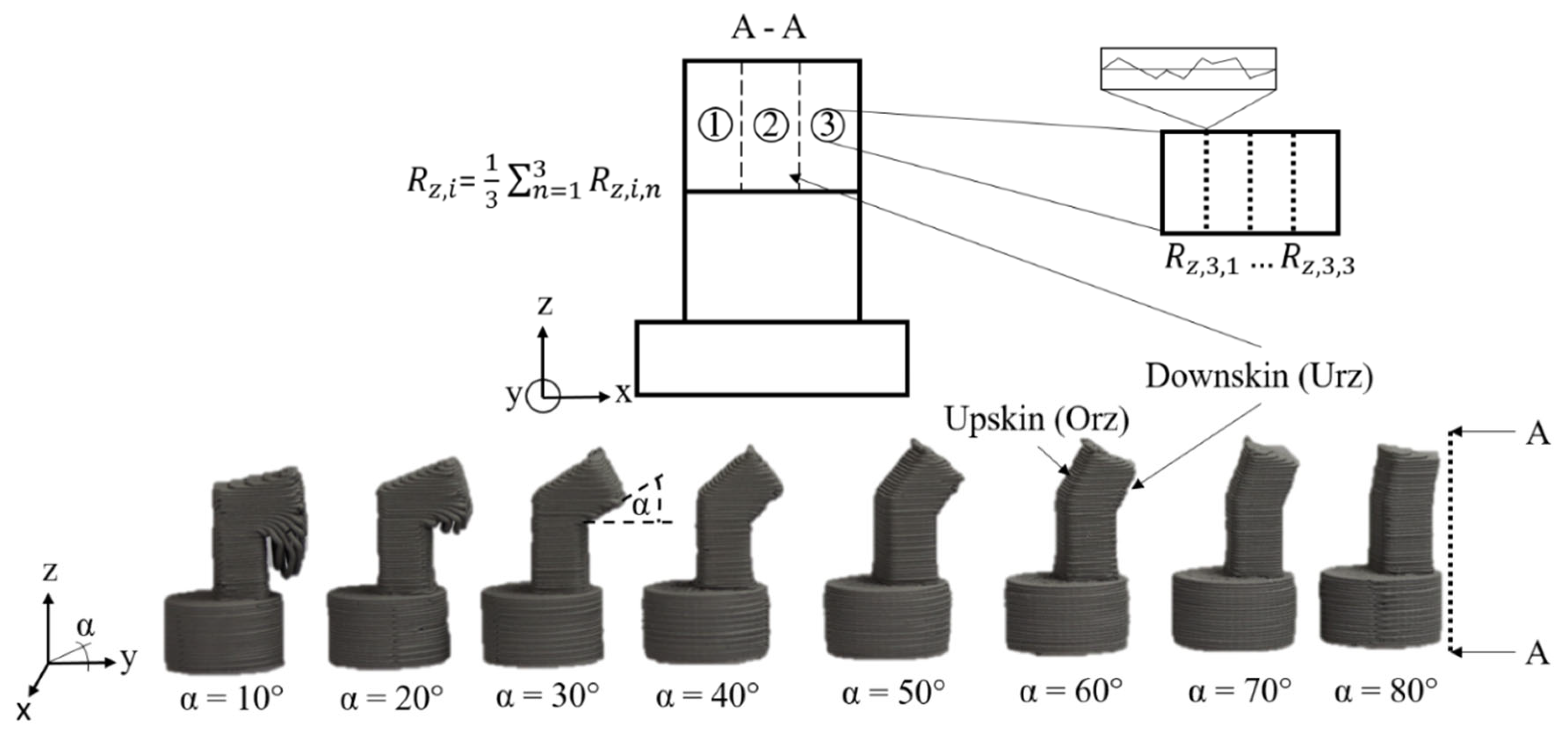
For the data preparation different overhang specimen (see Figure 1) have been manufactured on a Renkforce RF2000 (Conrad Electronic SE, Hirschau, Germany) 3D printer with a 0.4 mm nozzle using AISI 316L filament (PT&A GmbH, Dresden Germany) with 2.85 mm in diameter. The surface roughness of the greenpart specimen have been measured on the downskin (URz) and upskin (ORz) area of the overhang parts using a Keyence VHX-S600E (Osaka, Japan). Three areas of each side have been measured for three times and the average of the values has been taken as the average surface roughness of the downskin and upskin area.

Figure 1. Overhang specimen (green part) and roughness measuring procedure based on [23].

Figure 1. Overhang specimen (green part) and roughness measuring procedure based on [23].

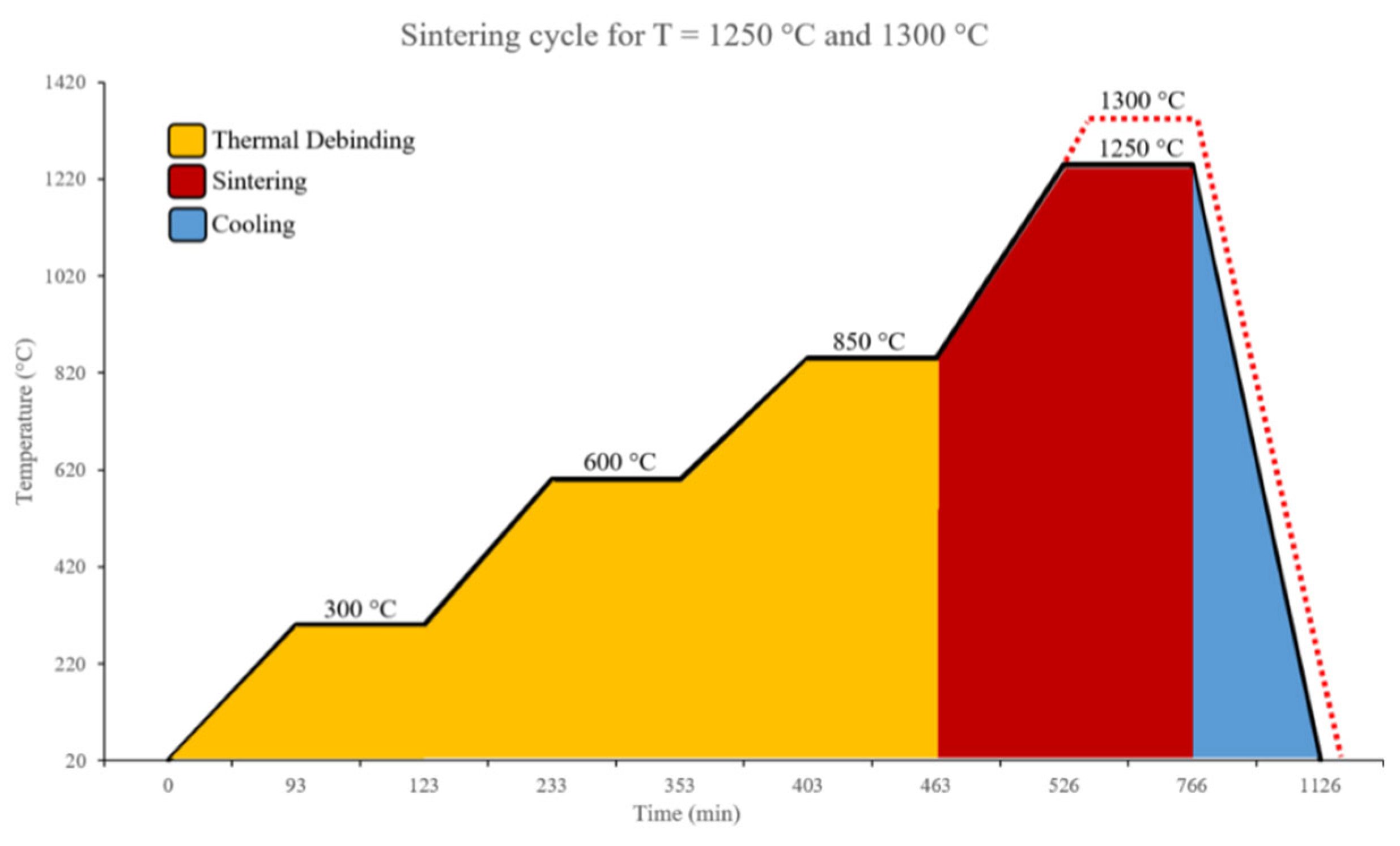
The starting powder composition is shown in [24]. The exact binder composition and particle size distribution of the metal powder are not provided by the manufacturer. The solvent debinding step is performed in 500 ml of acetone for 12 hours, heated at 38 °C, as recommended by the filament provider to achieve a 5% mass loss and open the pores for the thermal debinding step. The SEM image of the debinded 316L filament is provided in [25]. The particle size is in the range of 2 µm to 15 µm. An ExSO90 sinter oven (Aim3D GmbH, Rostock, Germany) was used for the thermal debinding and sintering step of the specimen. The thermal debinding and sintering cycles are performed in a combined single step according to the recommendation of the feedstock provider, with 99.9% Argon used as the atmosphere for both process steps at a flow rate of 1 l/min. It was found that this setup achieved a sintered density of 97.4% for the 316L specimen, which is higher than the metal injection molding (MIM) standard of 95% density [25]. Figure 2 illustrates the thermal debinding and sinter cycle for the specimen. Two different maximum temperatures were chosen for the printed process parameters. The holding temperatures of 300°C, 600°C, and 850°C were selected to burn out the binder from the samples. The heating rate between each holding temperature is 5 K/min.

Figure 2. Thermal debinding and sintering cycle for maximum sinter temperature of 1250 °C and 1300 °C on the basis of [25].

Figure 2. Thermal debinding and sintering cycle for maximum sinter temperature of 1250 °C and 1300 °C on the basis of [25].

The measurements of the different parameter combinations are depicted on the x-axis in Figure 3. On the y-axis, the different roughness measurements of the upskin and downskin surfaces are illustrated. The identification of individual samples was based on the set process parameters. The first number represents the infill percentage [%], the second number denotes the printing speed in millimeters per second [mm/s], the third number corresponds to the layer height in millimeters [mm], and the last number indicates the overhang angle in degrees [°]. For example, the combination 100;2100;0.2:10 signifies that the sample was printed with an infill of 100%, a printing speed of 2100 mm/s, and a layer height of 0.2 mm. The overhang angle of the sample is 10°. As expected, the mean surface roughness for the upskin and downskin areas is higher for lower overhang angles, independent of the printing speed and the percentage infill. A layer height of 0.4 mm causes higher surface roughness for the downskin and upskin areas. The roughness measurements are in the typical range for roughness in the MEX/M process [24].

Figure 3. Average surface roughness of the downskin and upskin are for each process parameter combination of the green parts.Furthermore, combinations of additional overhang angles have been printed, debinded, and sintered using the illustrated cycles (Figure 2). Table 1 shows the additional variations of the specimen parameters. The process parameters that were not varied are kept constant according to [24].

Figure 3. Average surface roughness of the downskin and upskin are for each process parameter combination of the green parts.Furthermore, combinations of additional overhang angles have been printed, debinded, and sintered using the illustrated cycles (Figure 2). Table 1 shows the additional variations of the specimen parameters. The process parameters that were not varied are kept constant according to [24].

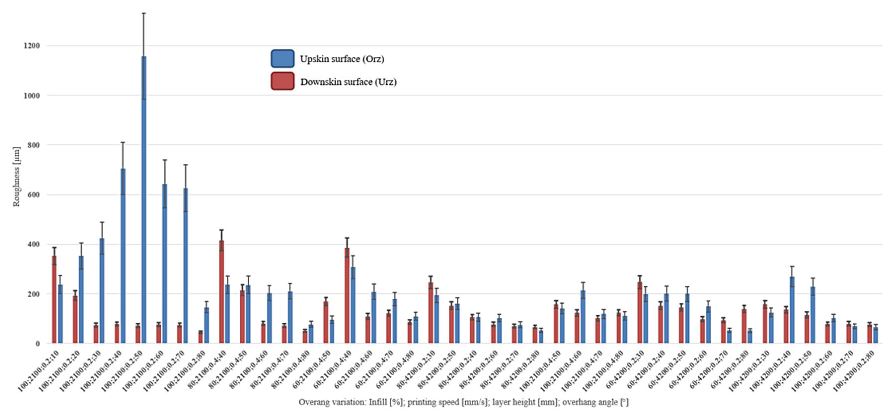
Table 1. Parameter variation of the experimental data.

Variation	Infill [%]	Printing speed [mm/s]	Layer height [mm]	Overhang angle [°]	Sintering temperature
Greenpart: 40 combinantions	60, 80, 100	2100, 4200	0.2, 0.4	10, 20, …, 80	-
Sinterpart: 48 combinations	50, 100	2100, 4200	0.2, 0.4	10, 20, …, 80	1250, 1300

Table 1. Parameter variation of the experimental data.

Variation	Infill [%]	Printing speed [mm/s]	Layer height [mm]	Overhang angle [°]	Sintering temperature
Greenpart: 40 combinantions	60, 80, 100	2100, 4200	0.2, 0.4	10, 20, …, 80	-
Sinterpart: 48 combinations	50, 100	2100, 4200	0.2, 0.4	10, 20, …, 80	1250, 1300

2.2. ML Development and Evaluation

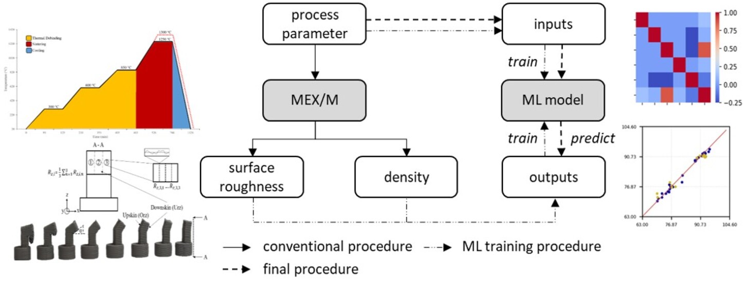
The applied methodology and relations between process and parameters is shown in Figure 4. The left side shows the current procedure where process parameters are selected, a MEX/M process is performed and the target parameters are investigated. The right side shows the target methodology where the process parameters are directly fed into the ML model to predict the resulting surface roughness and density. This procedure enables an initial assessment of the part quality without the part actually having to be manufactured.

Figure 4. Methodical scheme of the experimental approach and the ML prediction.

Figure 4. Methodical scheme of the experimental approach and the ML prediction.

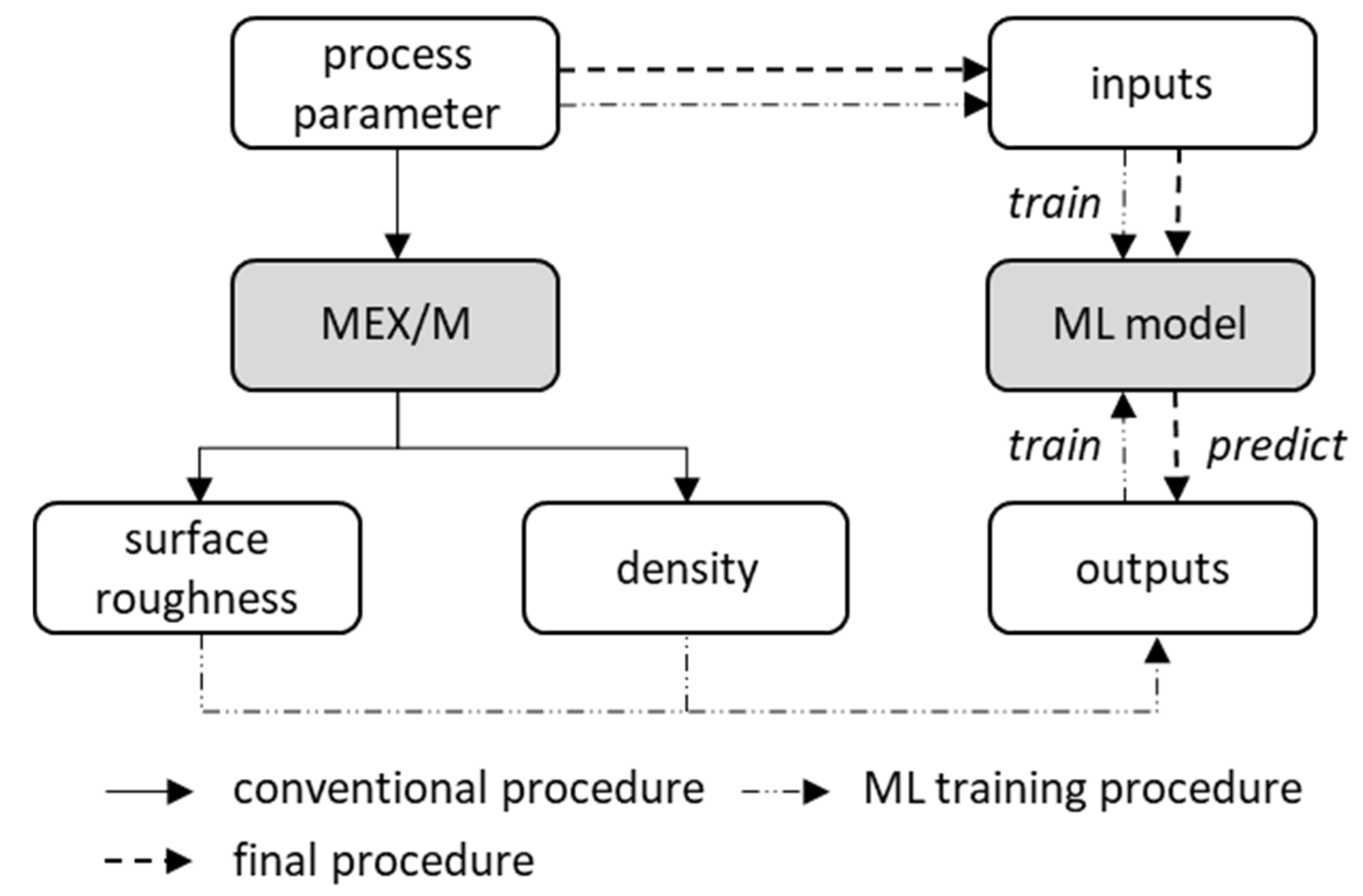
The inputs and outputs of the ML model are derived from the process. The process parameters of the MEX/M process are used as inputs and the part properties as outputs. The considered parameters are summarized in Table 2.

Table 2. Input and output parameter for the investigated ML models.

Parameter	Symbol	Description	Unit	Model
Inputs
infill	fill	percentage of the material fill level	%	URz, ORz, density
print speed	v	speed of printing head during the process	mm/min
layer thickness	l	height of the individual print layers	mm
overhang angle	alpha	Overhang angle of unsupported areas of the printed part	°
sinter temperature	st	temperature used when sintering the material	°C	density
outputs
Downskin surface roughness	URz	measured average bottom inclined wall roughness of the component surface	µm	URz
Upskin surface roughness	ORz	measured average top inclined wall roughness of the component surface	µm	ORz
density	rho	part density before sintering	%	density

Table 2. Input and output parameter for the investigated ML models.

Parameter	Symbol	Description	Unit	Model
Inputs
infill	fill	percentage of the material fill level	%	URz, ORz, density
print speed	v	speed of printing head during the process	mm/min
layer thickness	l	height of the individual print layers	mm
overhang angle	alpha	Overhang angle of unsupported areas of the printed part	°
sinter temperature	st	temperature used when sintering the material	°C	density
outputs
Downskin surface roughness	URz	measured average bottom inclined wall roughness of the component surface	µm	URz
Upskin surface roughness	ORz	measured average top inclined wall roughness of the component surface	µm	ORz
density	rho	part density before sintering	%	density

For data processing and training of the models python (v3.8.19) was used with the scikit-learn library (v1.3.0) [26]. These environments were selected to ensure compatibility with the latest machine learning methods as well as robust and efficient processing of the data. The developed suitable ML models and the experimental data are provided in source [27].

3. ML Model Setup & Training

The data set generated for the investigation of surface roughness consists of 40 data points, while the data set for density comprises 48 data points. The preprocessing of the data consists of four steps: cleaning the data by removing outliers and making sure no values are missing, investigating correlations between features and labels and removing strongly correlated features if necessary, splitting the data into training and test set and finally scaling the input data to ensure similar magnitudes of feature values.

When cleaning the data, no missing values and only slight outliers where detected. As the data set is already very small, it was decided not to remove any further data points as long as the outliers are not attributable to measurement errors. Subsequently, a correlation analysis was performed, including the calculation of the correlation matrix and the Spearman coefficients [28,29]. The plots in Figure 5 show the correlation matrices for the parameters. The calculated coefficients are summarized in Table 3. The results show that URz correlates significantly negatively with angle (-0.63), while ORz also shows a strong negative correlation with print speed ( -0.5) and angle (-0.58). Density shows a strong positive correlation with infill (0.87).

Figure 5. Correlation matrices for the surface roughness (left) and density (right).

Figure 5. Correlation matrices for the surface roughness (left) and density (right).

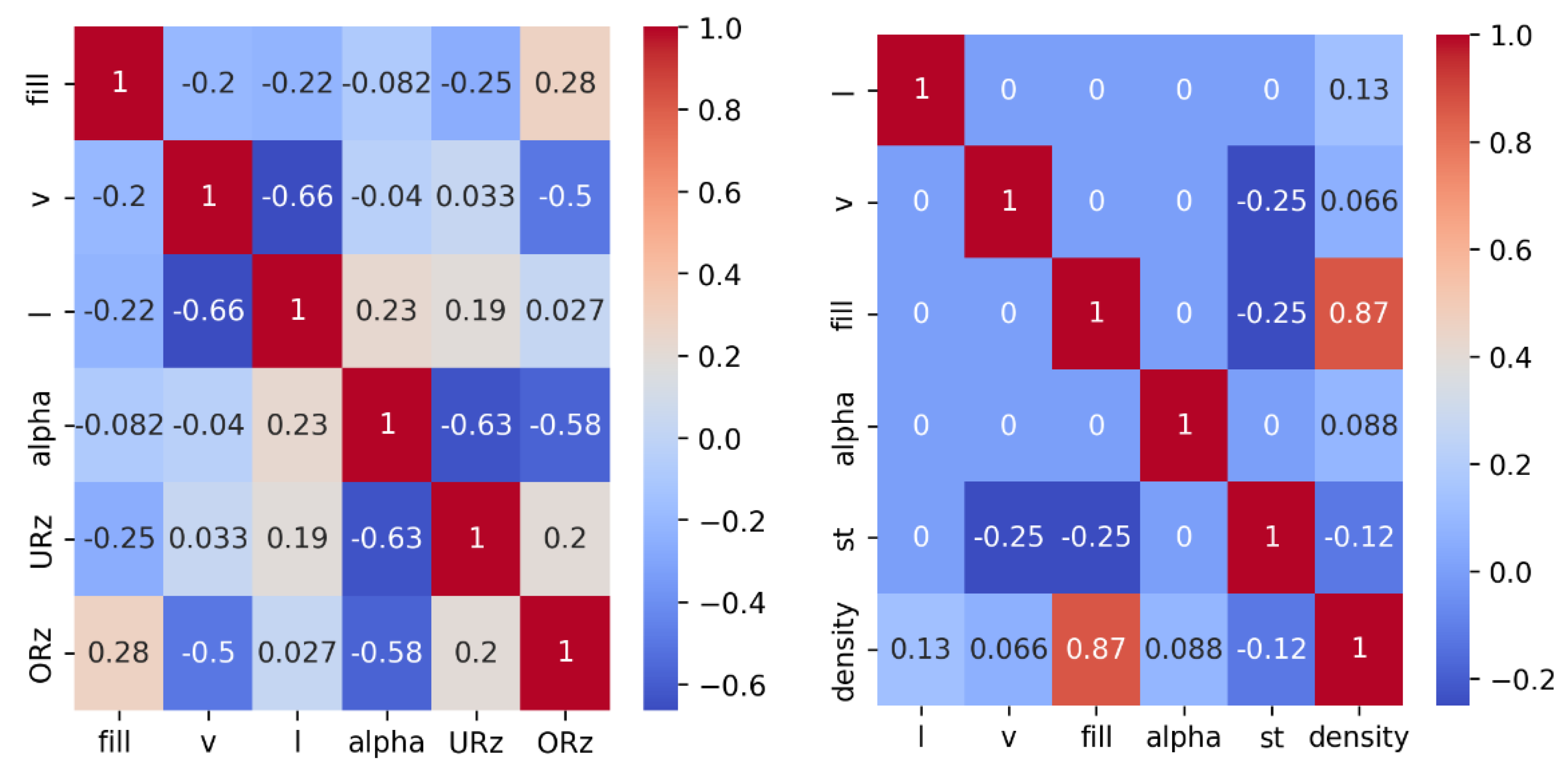
Table 3. Spearmen coefficients for the downskin surface roughness, upskin surface roughness and density.

	URz	ORz	Density
fill	-0.25	0.28	0.87
v	0.03	-0.5	0.07
l	0.19	0.03	0.13
alpha	-0.63	-0.58	0.09
st	-	-	-0.12

Table 3. Spearmen coefficients for the downskin surface roughness, upskin surface roughness and density.

	URz	ORz	Density
fill	-0.25	0.28	0.87
v	0.03	-0.5	0.07
l	0.19	0.03	0.13
alpha	-0.63	-0.58	0.09
st	-	-	-0.12

For processing in ML algorithms, the data is split into a training and test data set in a ratio of 75% to 25%. A stratified shuffle is applied based on the respective output parameter in order to take the distribution of the target variables into account. This ensures that, despite the small amount of data, results over the entire interval of the target parameter are always included in the training and test data set. In addition, polynomial features are calculated up to the second degree in order to capture interaction effects [30]. When training the models, it is investigated whether the inclusion of polynomial features offers added value. A feature selection is carried out using SelectKBest. To standardize the feature values, either MinMax or Standard scaling is used to normalize the number spaces to a comparable range, which is important for the accuracy of some ML algorithms [26,31].

The selection of algorithms for model training was based on the criteria of robustness, prediction accuracy and interpretability. The models considered include linear regression (LR) based on its simplicity and good interpretability for linear relationships [32], random forest regressor (RFR) due to its robustness to outliers and their ability to model non-linear relationships [33], support vector machines (SVM) because its suitable for small data sets and offers good generalization capabilities [34], k-nearest-regressor (kNN) based on its simple implementation and adaptation to non-linear structures [35,36], multilayer perceptron (MLP) for potentially more complex correlations and pattern recognition [37,38,39] and finally a bagging regressor (Bag) with kNN [40], decision tree regressors or MLP as base estimators to reduce the variance and increase the stability of the model.

To train the models a pipeline was defined that includes the following steps: polynomial features, SelectKBest, scaling and the respective estimator. To evaluate the model performance the RMSE and the R² value were defined as common error measures [41], supplemented by a qualitative evaluation using plots of the correct versus the predicted values. The RMSE is given in the respective unit of the target value - µm for URz and ORz and percentage points in % for density. RMSE and R² are defined in [10].

To optimize the models, hyperparameter tuning is performed using gridsearch (GridSearchCV) [26] with cross-validation (CV). The corresponding parameter spaces are given for each algorithm in Table 4. All pipelines consider a variation of the scaler, SelectKBest and polynomial features in the gridsearch.

Table 4. Selected hyperparameter for all investigated ML models.

Algorithm		Parameter	Values
polynomial features		activated	True, False
KBest		k	5, 10, 15, 'all'
scaler		scaler	MinMaxScaler(), StandardScaler()
estimator	RFR	n_estimators	10, 50, 100
		max_depth	None, 2, 5, 10
		min_samples_leaf	1, 2, 3
		min_samples_split	2, 5
		max_features	None, sqrt
		bootstrap	True, False
	kNN	n_neighbors	3, 5, 7
		weights	uniform, distance
		algorithm	auto, ball_tree, kd,_tree
		p	1, 2
	MLP	hidden_layer_sizes	(10,), (20,), (10, 10,), (25, 25,)
		alpha	0.0001, 0.001, 0.01
		activation	relu, tanh
		solver	lbfgs, adam
		learning_rate	constant, adaptive
	Bag	estimator	kNN, DTR, MLP
		n_estimators	5, 10, 20
		max_samples	0.5, 0.7, 1.0
		bootstrap	True, False
		bootstrap_features	True, False

Table 4. Selected hyperparameter for all investigated ML models.

Algorithm		Parameter	Values
polynomial features		activated	True, False
KBest		k	5, 10, 15, 'all'
scaler		scaler	MinMaxScaler(), StandardScaler()
estimator	RFR	n_estimators	10, 50, 100
		max_depth	None, 2, 5, 10
		min_samples_leaf	1, 2, 3
		min_samples_split	2, 5
		max_features	None, sqrt
		bootstrap	True, False
	kNN	n_neighbors	3, 5, 7
		weights	uniform, distance
		algorithm	auto, ball_tree, kd,_tree
		p	1, 2
	MLP	hidden_layer_sizes	(10,), (20,), (10, 10,), (25, 25,)
		alpha	0.0001, 0.001, 0.01
		activation	relu, tanh
		solver	lbfgs, adam
		learning_rate	constant, adaptive
	Bag	estimator	kNN, DTR, MLP
		n_estimators	5, 10, 20
		max_samples	0.5, 0.7, 1.0
		bootstrap	True, False
		bootstrap_features	True, False

For the training of the ML model, a statistical evaluation was performed, starting with a gridsearch-based parameter tuning. The search over the respective parameter spaces is performed 10 times each. The best configurations are then selected. The models are then trained 50 times with the selected parameter combinations and the mean error is determined. This procedure ensures optimal parameter selection and checks the robustness of the model.

4. ML Results

The various ML models LR, RFR, SVM, kNN, MLP and Bag were trained and evaluated with hyperparameter tuning. Subsequently, the R² factor and the RSE for downskin and upskin angle of the experimental data were evaluated (compare Figure 3). Table 5 shows the respective values of each model. The highest R² value in the training data set can be seen in the MLP model for the URz.

RFR and Bag also show a high value of 0.86 and 0.9. Similarly, these models also have a low RMSE value for the training data (MLP 18.75 µm, RFR 32.04 µm and Bag 27.15 µm). A similar observation can be made in the training data set for ORz, in which MLP (0.99) also has the highest R² value, followed by RFR (0.88) and Bag (0.75). SVM has the lowest R² value in the training data set for URz with 0.44 followed by LR with a value of 0.55. The RMSE value is highest for SVM at 63.79 µm and for LR at 57.44 µm. In the case of ORz, the R² factor is also lowest for SVM with 0.26 and also followed by LR with 0.58. Here the RMSE value is 144.90 µm (SVM) and 109.34 µm (LR). In the test dataset, the RFR model achieved a maximum coefficient of determination (R²) of 0.7 for the target variable URz, while the kNN model attained an R² value of 0.65. The corresponding RMSE values were 51.27 µm and 47.52 µm, respectively. For the target variable ORz, the kNN model also recorded the highest R² value of 0.69, with an RMSE value of 170.96 µm.

Table 5. R² value and RMSE of URz and ORz in training and test case for all ML models.

Model	Target value	Indicators	Training	Test
LR	URz	R²	0.55	0.51
		RMSE [µm]	57.44	60.21
	ORz	R²	0.58	0.41
		RMSE [µm]	109.34	237.45
RFR	URz	R²	0.86	0.70
		RMSE [µm]	32.04	47.51
	ORz	R²	0.89	0.31
		RMSE [µm]	56.79	255.7
SVM	URz	R²	0.44	0.39
		RMSE [µm]	63.79	67.60
	ORz	R²	0.26	0.1
		RMSE [µm]	144.90	293.12
kNN	URz	R²	0.66	0.65
		RMSE [µm]	49.80	51.27
	ORz	R²	0.73	0.69
		RMSE [µm]	87.98	170.96
MLP	URz	R²	0.95	0.26
		RMSE [µm]	18.76	74.66
	ORz	R²	0.99	0.13
		RMSE [µm]	13.71	288.44
bag	URz	R²	0.90	0.53
		RMSE [µm]	27.15	59.10
	ORz	R²	0.75	0.60
		RMSE [µm]	84.63	194.01

Table 5. R² value and RMSE of URz and ORz in training and test case for all ML models.

Model	Target value	Indicators	Training	Test
LR	URz	R²	0.55	0.51
		RMSE [µm]	57.44	60.21
	ORz	R²	0.58	0.41
		RMSE [µm]	109.34	237.45
RFR	URz	R²	0.86	0.70
		RMSE [µm]	32.04	47.51
	ORz	R²	0.89	0.31
		RMSE [µm]	56.79	255.7
SVM	URz	R²	0.44	0.39
		RMSE [µm]	63.79	67.60
	ORz	R²	0.26	0.1
		RMSE [µm]	144.90	293.12
kNN	URz	R²	0.66	0.65
		RMSE [µm]	49.80	51.27
	ORz	R²	0.73	0.69
		RMSE [µm]	87.98	170.96
MLP	URz	R²	0.95	0.26
		RMSE [µm]	18.76	74.66
	ORz	R²	0.99	0.13
		RMSE [µm]	13.71	288.44
bag	URz	R²	0.90	0.53
		RMSE [µm]	27.15	59.10
	ORz	R²	0.75	0.60
		RMSE [µm]	84.63	194.01

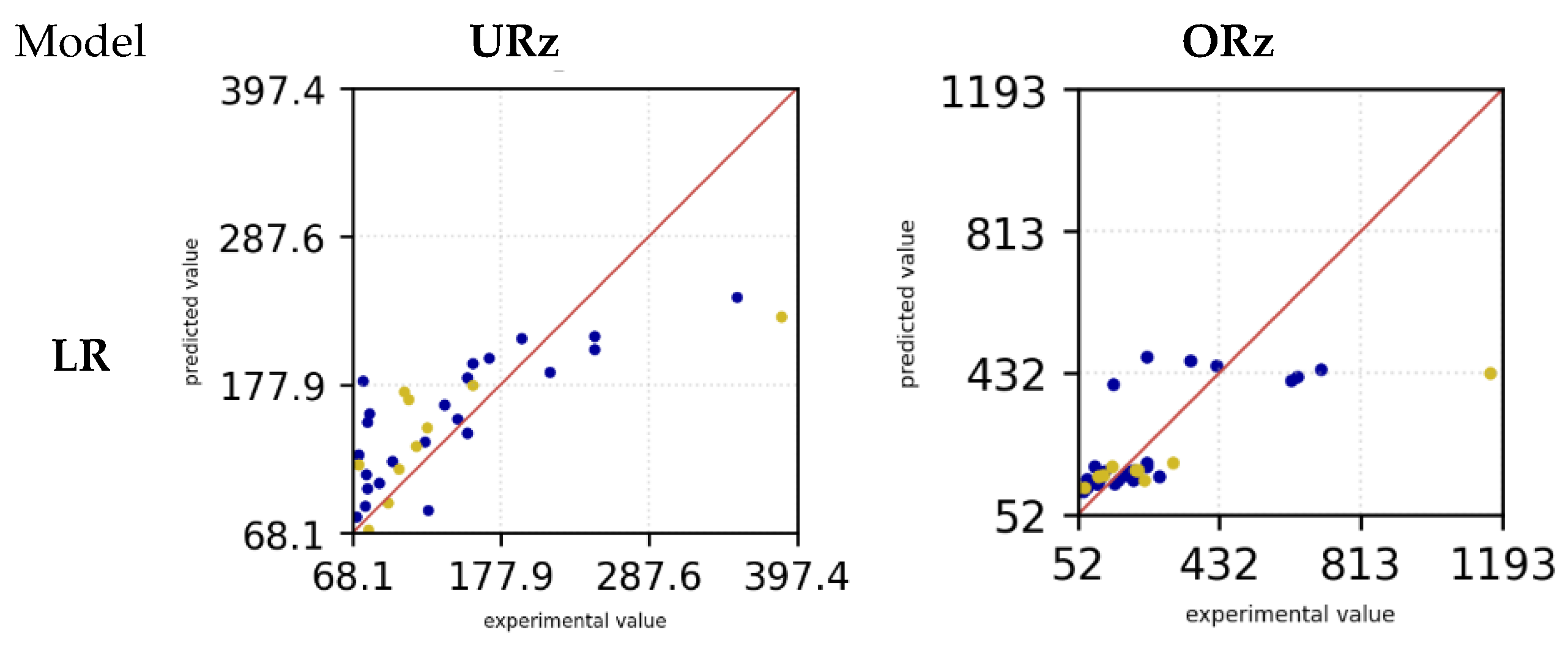
Additionally, diagrams of the respective models were generated, illustrating the predictions compared to the experimental data. The red line indicates a perfect prediction. The farther the points are from the line, the less accurate the predictions are. Figure 6 presents the prediction diagrams of the models under examination, facilitating an initial selection of the models in question. The blue dots depict the training data, while the yellow dots represent the test data. For the LR model, it is observed that both the test and training data predictions deviate from the experimental data. This phenomenon is observable for both the downskin angle URz and the upskin angle ORz. Only for small overhang angles do the predictions appear to align more closely with the experimental data, resulting in smaller deviations for both URz and ORz. The SVM model exhibits a behavior similar to that of the LR model's predictions. In this instance as well, the predictions significantly deviate from the actual values. Both the LR and SVM models tend to underestimate the actual surface roughness for URz and ORz. In contrast, the RFR model demonstrates higher accuracy in predicting the training data with larger URz values, a trend that is also observed in the test data. Nonetheless, in both scenarios, the roughness prediction is underestimated.

Figure 6. Surface roughness prediction versus experimental measurements in [µm] for the training (blue) and test data (yellow) of all investigated ML models.

Figure 6. Surface roughness prediction versus experimental measurements in [µm] for the training (blue) and test data (yellow) of all investigated ML models.

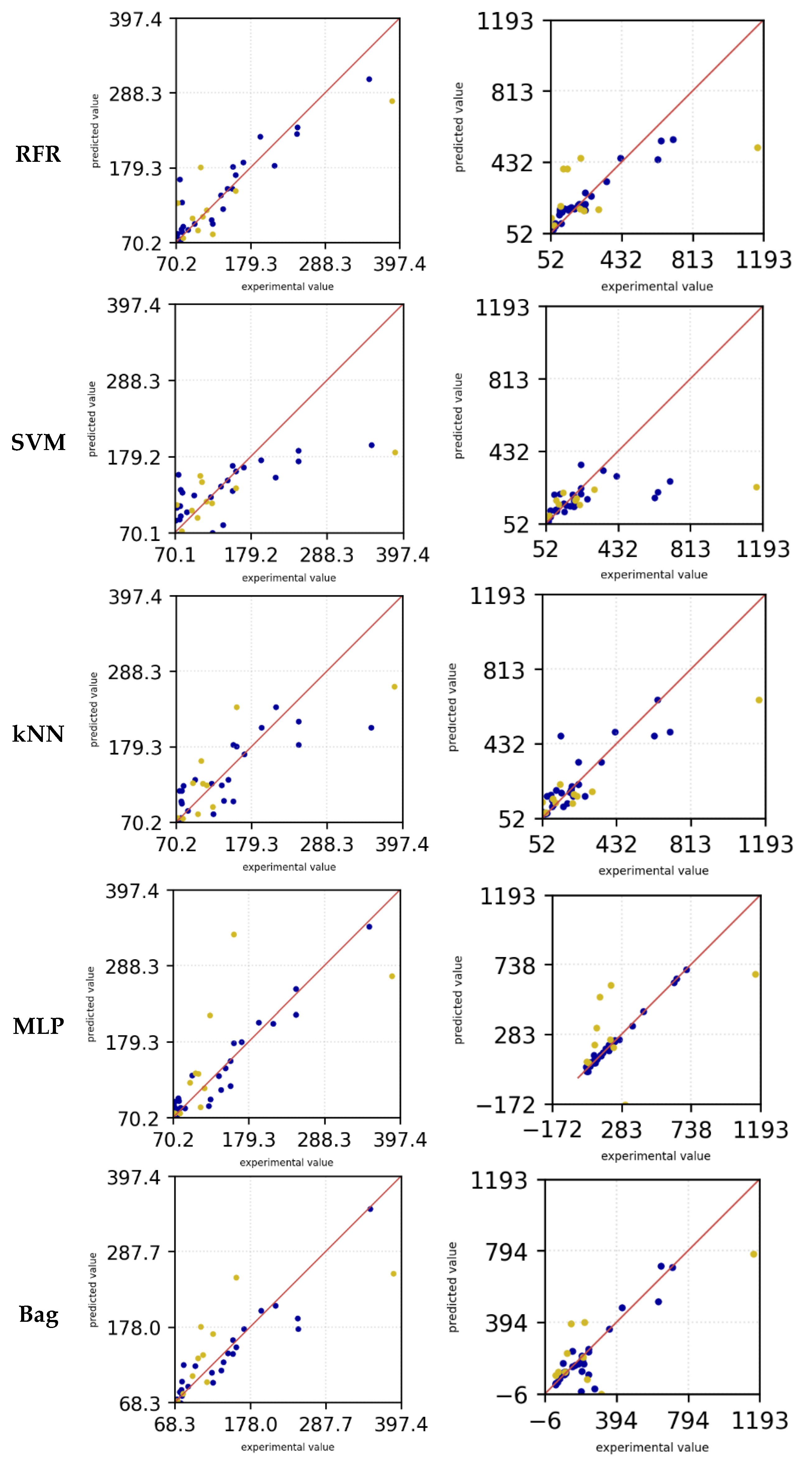
The kNN model demonstrates that more accurate predictions can be achieved for low URz and Orz values. However, for higher roughness, the predictions deviate from the experimental data. In this context, both the training and test datasets underestimate the actual values for lager roughness values (> 200 µm). The bag model exhibited a high level of predictive accuracy for Urz in the training dataset, including for large roughness values. Nevertheless, for small roughness values, the model showed a tendency to overestimate predictions in the test dataset, whereas for large roughness values, it occasionally underestimated the predictions. In the case of Orz, the training data is even more accurate in its prediction and tends to underestimate small roughness values.

The test data overestimates the experimental data and predict higher values for the roughness. However, for large roughnesses, the predictions in the test data set tend to be underestimated. In the training dataset, the MLP model shows the smallest deviations in the predicted values for both Orz and Urz. Only in the test data, small roughnesses are overestimated and larger roughnesses are underestimated.

Since the training data for MLP and Bag are heavily aligned with the experimental data, while the test data fluctuate more around the exact prediction, the machine learning models appear to be overfitted. For Urz and Orz, the MLP model appears to perform the best despite signs of overfitting and is therefore selected for further parameter optimization. The other algorithms are not further investigated as the MLP seems to be the most promising algorithm for this dataset.

The same approach was applied to the target variable density, where, with parameter optimization using polynomial feature importances and the SelectKBest method, the Bag model appears to be the best starting point. The prediction diagram is shown in Figure 7. It can be observed that the predictions for both the training data and the test data are located close to the actual values. Occasionally, the predictions for the training data are underestimated, which may indicate that overfitting is not occurring. Both training and test data oscillate within a similar range around the optimal axis, which means that a good generalization of the model can be assumed. In the following only the Bag model will be investigated further for the density prediction.

Figure 7. Density prediction versus experimental measurements in % points for the training (blue) and test data (yellow).

Figure 7. Density prediction versus experimental measurements in % points for the training (blue) and test data (yellow).

The hyperparameter optimization over 10 runs using polynomial feature importances and SelectKBest led to the following results in terms of the R² factor and RMSE for Urz, Orz and density (see Table 6). A direct comparison with Table 5 for the MLP model shows a significant increase in the R² value from 0.25 to approximately 0.71. Additionally, the RMSE was reduced by more than 25 µm to around 49.27 µm. Although the R² factor in the training dataset decreased to 0.83 and the RMSE increased to 34.82 µm, the model initially seemed to be overfitted, so the optimization counteracted this trend. The standard deviation of the R² value for Urz is 0.11 for the training data and 0.3 for the test data. Thus, the variability among the training data is less than that of the test data. This suggests variability in the model’s performance and indicates the need for further iterations to achieve a more robust R² value. The RMSE for both the training data and test data also exhibits significant variability, making it difficult to draw definitive conclusions about the error of the mean values after 10 iterations. This variability suggests that the MLP model is sensitive to the hyperparameters, necessitating further optimization iterations to achieve greater robustness.

A similar observation can be made for the ORz MLP model. Here, the R² value decreases from 0.99 to 0.72 and the RMSE increased from 13.71 µm to approximately 90.8 µm in the training dataset from the initial iteration step (compare Table 5). The R² value for the test data, on the other hand, increases from 0.12 to around 0.46 and the RMSE error is reduced to 222.92 µm. The reduction of the R² value in the training data is an indication that overfitting is counteracted, but the high standard deviation of R² and RMSE indicates a low robustness of the model.

The bag model was used for the den”Ity ’orecast. In the training data set as well as in the test data set, the R² value is already high at 0.96 and 0.91, so that the independent variables can be well described by the number of dependent variables. The standard deviation is also much smaller than for the other two MLP models, which means that the model can be expected to be more robust. The same applies to the RMSE error, which is small at 1.64 % (training) and 2.53 % (test) and also has a standard deviation of less than 0.55 %.

Table 6. Hyperparameter optimization after 10 iterations for the MLP and Bag models.

	Value	Urz (MLP)	Orz (MLP)	Density (Bag)
Train	R2	0.83 ± 0.11	0.72 ± 0.12	0.96 ± 0.02
	RMSE	34.82 ± 13.82 [µm]	90.8 ± 34.7 [µm]	1.64 ± 0.34 [%]
Test	R2	0.71 ± 0.3	0.46 ± 0.15	0.91 ± 0.04
	RMSE	49.27 ± 18.95 [µm]	222.92 ± 41.41 [µm]	2.53 ± 0.53 [%]

Table 6. Hyperparameter optimization after 10 iterations for the MLP and Bag models.

	Value	Urz (MLP)	Orz (MLP)	Density (Bag)
Train	R2	0.83 ± 0.11	0.72 ± 0.12	0.96 ± 0.02
	RMSE	34.82 ± 13.82 [µm]	90.8 ± 34.7 [µm]	1.64 ± 0.34 [%]
Test	R2	0.71 ± 0.3	0.46 ± 0.15	0.91 ± 0.04
	RMSE	49.27 ± 18.95 [µm]	222.92 ± 41.41 [µm]	2.53 ± 0.53 [%]

After completing 10 iterations, the optimal hyperparameters were determined by maximizing the coefficient of determination and minimizing the root mean square error. Table 7 shows the values with the optimized hyperparameters. The selected hyperparameters for the MLP model are illustrated in Table 8 and for the Bag model in Table 9.

An R² of 0.96 shows that the model can explain 96 % of the variance of the surface roughness (Urz) in the training. The RMSE error is also significantly lower here at 16.04 µm. In the test data set, the R² factor was also increased to 0.88 and also has a low RMSE value of 32.11 µm. A significant increase in the error on the test data indicates that the model has difficulties predicting the test data with the same precision as the training data. There is a possibility of a slight overfitting effect occurring in this case. The R² factor with 0.91 does not change for Orz. A constant R² value indicates that the model has learned the patterns in the data well and also transfers them to the test data. An RMSE increase from 51.29 µm (training) to 91.89 µm (test) strongly indicates overfitting. Regularization, optimized data processing and model adjustments can improve the generalization and reduce the test error. For the bag model for density, the R² value for 0.98 (training) and 0.95 (test) is also high. The RMSE error is lower in the training (1.12 %) than in the test (1.97 %). Further optimization iterations should reduce the different errors.

Table 7. Parameter optimization (best models).

	Value	Urz (MLP)	Orz (MLP)	Density (Bag)
Train	R2	0.96	0.91	0.98
	RMSE	16.04 [µm]	51.29 [µm]	1.12 [%]
Test	R2	0.88	0.91	0.95
	RMSE	32.11 [µm]	91.89 [µm]	1.97 [%]

Table 7. Parameter optimization (best models).

	Value	Urz (MLP)	Orz (MLP)	Density (Bag)
Train	R2	0.96	0.91	0.98
	RMSE	16.04 [µm]	51.29 [µm]	1.12 [%]
Test	R2	0.88	0.91	0.95
	RMSE	32.11 [µm]	91.89 [µm]	1.97 [%]

Table 8. Parameter optimization (selected hyperparameter) – Urz, Orz.

Algorithm	Parameter	Urz	Orz
polynomial features	activated	False	True
Kbest	K	-	10
scaler	scaler	MinMaxScaler	MinMaxScaler
estimator	model	MLP
hyperparameters	hidden_layer_sizes	(10,)	(10,)
	alpha	0.01	0.01
	activation	relu	relu
	solver	lbfgs	lbfgs
	learning_rate	adaptive	adaptive

Table 8. Parameter optimization (selected hyperparameter) – Urz, Orz.

Algorithm	Parameter	Urz	Orz
polynomial features	activated	False	True
Kbest	K	-	10
scaler	scaler	MinMaxScaler	MinMaxScaler
estimator	model	MLP
hyperparameters	hidden_layer_sizes	(10,)	(10,)
	alpha	0.01	0.01
	activation	relu	relu
	solver	lbfgs	lbfgs
	learning_rate	adaptive	adaptive

Table 9. Parameter optimization (selected hyperparameter) – density.

Algorithm	Parameter	Density
polynomial features	activated	True
Kbest	K	15
scaler	scaler	StandardScaler
bag	estimator	DecisionTreeRegressor
	n_estimators	10
	max_samples	0.7
	bootstrap	false
	bootstrap_features	True

Table 9. Parameter optimization (selected hyperparameter) – density.

Algorithm	Parameter	Density
polynomial features	activated	True
Kbest	K	15
scaler	scaler	StandardScaler
bag	estimator	DecisionTreeRegressor
	n_estimators	10
	max_samples	0.7
	bootstrap	false
	bootstrap_features	True

Table 10 indicates the averaged evaluation parameters of 50 iterations with the optimized hyperparameters. The observed discrepancy between training and test data indicates that the model performs better on the training set, which could suggest some degree of overfitting. However, the low standard deviation across both datasets demonstrates a high level of robustness and consistency in the model’s predictions. For Orz, the R² factor is 0.94 in the training dataset and 0.73 in the test dataset, with a standard deviation of 0.07. Although the performance on the test data is lower, the small standard deviation highlights the stability of the model across samples and deliver similar results. Similarly, for density, the R² factor is 0.98 on the training set with a standard deviation of 0.003, and 0.92 on the test set with a standard deviation of 0.02. This consistency in performance, coupled with the relatively small deviations, reinforces the robustness of the model, even if the performance on the test data does not reach the same level as on the training data. Overall, while there is evidence of better training data performance, the low standard deviations suggest that the model’s predictions are reliable and not overly sensitive to variations within the datasets. For the RMSE, the error for Urz during training is 14.32 with a standard deviation of 3.27, reflecting improvements compared to the results obtained after hyperparameter optimization with 10 iterations. Furthermore, the error in the test set was reduced to 34.93, accompanied by a standard deviation of 6.28. These results indicate that the optimization process enhanced both the accuracy and stability of the predictions for Urz.

For Orz, the RMSE during training is 47.67 µm with a standard deviation of 16.45 µm. However, the test RMSE is significantly higher at 155.63 µm, with a standard deviation of 20.47 µm. This suggests that, while the model achieved reasonable performance in training, its ability to generalize to test data is more limited for Orz. Additionally, both the roughness and deviations are notably higher for Orz compared to Urz.

Importantly, despite the higher error and variability in the predictions for Orz, there was a reduction in standard deviation for both training and test datasets when compared to the results obtained after 10 iterations of hyperparameter optimization (as seen in Table 6). This improvement in stability indicates that the optimization process contributed to reducing variability in the predictions, even if the overall performance still shows room for improvement. For density, the RMSE in training is 1.06 % with a standard deviation of 0.11, while in the test dataset, it increases to 2.51 % with a deviation of 0.29 %. This indicates a noticeable performance drop when transitioning from training to test data. Furthermore, the test RMSE and its deviation are higher compared to the results after 10 iterations of hyperparameter optimization.

Table 10. Model training with best parameters (50 runs) – MLP, MLP und Bagging.

	Value	Urz (MLP)	Orz (MLP)	Density (Bag)
Train	R2	0.97 ± 0.01	0.94 ± 0.06	0.98 ± 0.003
	RMSE	14.32 ± 3.27 [µm]	47.67 ± 16.45 [µm]	1.06 ± 0.11 [%]
Test	R2	0.85 ± 0.06	0.73 ± 0.07	0.92 ± 0.02
	RMSE	34.93 ± 6.28 [µm]	155.63 ± 20.47 [µm]	2.51 ± 0.29 [%]

Table 10. Model training with best parameters (50 runs) – MLP, MLP und Bagging.

	Value	Urz (MLP)	Orz (MLP)	Density (Bag)
Train	R2	0.97 ± 0.01	0.94 ± 0.06	0.98 ± 0.003
	RMSE	14.32 ± 3.27 [µm]	47.67 ± 16.45 [µm]	1.06 ± 0.11 [%]
Test	R2	0.85 ± 0.06	0.73 ± 0.07	0.92 ± 0.02
	RMSE	34.93 ± 6.28 [µm]	155.63 ± 20.47 [µm]	2.51 ± 0.29 [%]

Using the selected hyperparameters from Table 8 and Table 9 for the MLP and Bag models, the corresponding values for RMSE and R² as best results are presented in Table 11. These results offer insights into how the optimized hyperparameters affect model performance in terms of accuracy and explanatory power. For Urz, the model demonstrated a strong fit with an R² of 0.96 in the training set, indicating that 96% of the variance in the data was explained. However, the test set R² decreased to 0.87, and the RMSE increased from 17.38 µm in training to 32.93 µm in testing, suggesting some overfitting. The Orz results showed a similar trend, with a high R² of 0.94 in the training set, but a significant drop to 0.79 in the test set. Additionally, the RMSE for Orz was substantially higher, moving from 41.58 µm in training to 138.99 µm in testing, indicating a severe generalization issue. In contrast, the model performed exceptionally well for density, achieving an R² of 0.99 in the training set and 0.95 in the test set, with an RMSE of 0.95% and 1.88%, respectively. The minimal difference between training and test RMSE for density suggests that the model generalizes well to unseen data. Overall, the results highlight that while the model is highly effective for density, additional improvements in feature selection and regularization are needed to enhance the generalization performance for Urz and especially Orz, where overfitting is more pronounced.

Table 11. Model training with best models (best models).

	Value	Urz (MLP)	Orz (MLP)	Density (Bag)
Train	R2	0.96	0.94	0.99
	RMSE	17.38 [µm]	41.58 [µm]	0.95 [%]
Test	R2	0.87	0.79	0.95
	RMSE	32.93 [µm]	138.99 [µm]	1.88 [%]

Table 11. Model training with best models (best models).

	Value	Urz (MLP)	Orz (MLP)	Density (Bag)
Train	R2	0.96	0.94	0.99
	RMSE	17.38 [µm]	41.58 [µm]	0.95 [%]
Test	R2	0.87	0.79	0.95
	RMSE	32.93 [µm]	138.99 [µm]	1.88 [%]

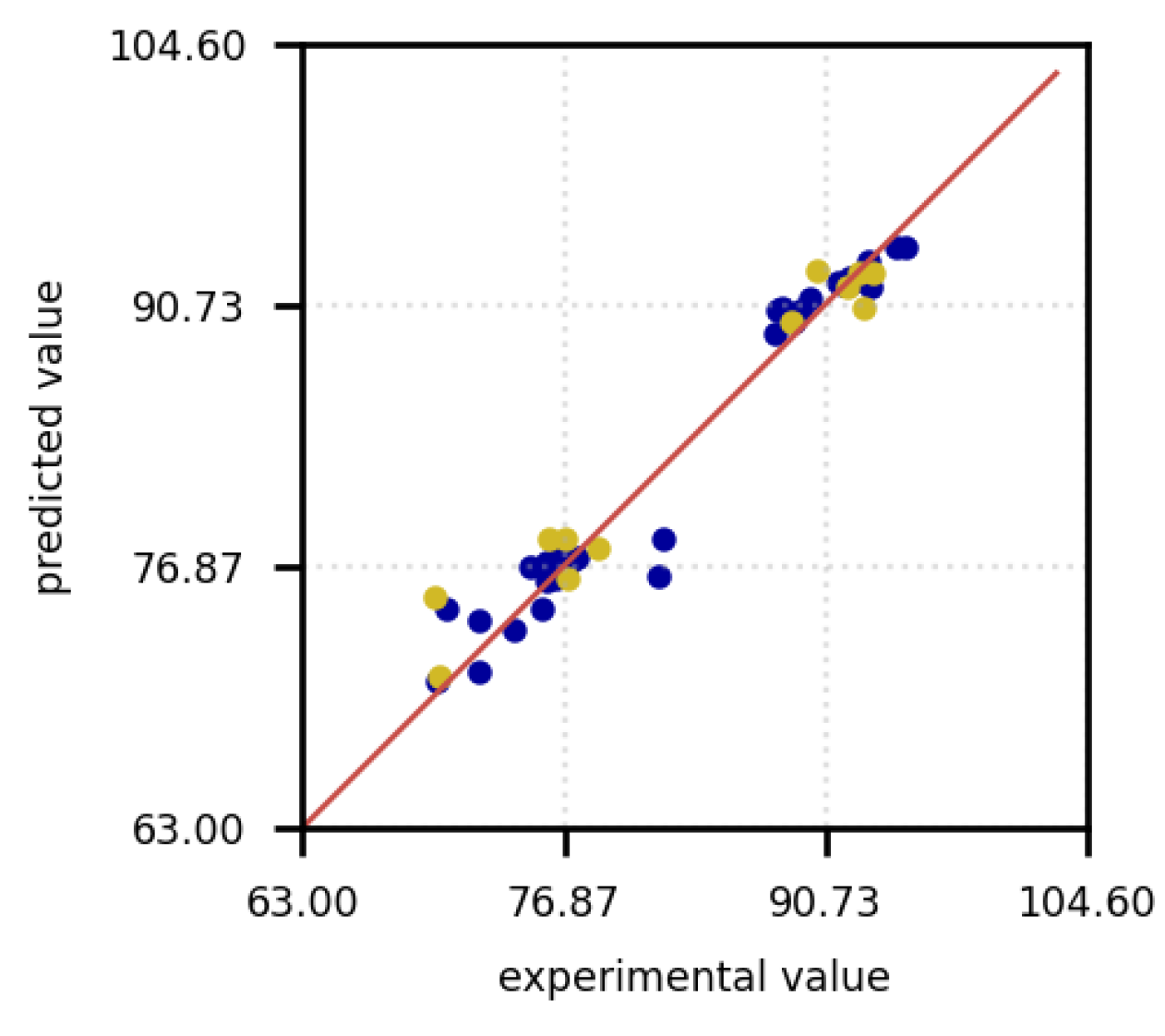
Figure 8 shows the predictions of the experimental values as a further evaluation criterion. In this case too, the blue dots are the training data set and the yellow dots are the test data. For Urz (left) it can be seen that the trending data for small roughness values deviate from the exact values and make precise predictions with increasing roughness. The scattering for small roughness values can be observed in the test data. With increasing roughness, a deviation from the experimental data can still be observed, but this deviation remains constant with increasing roughness values.

Figure 8. Surface roughness prediction versus experimental measurements for the training (blue) and test data (yellow) of all investigated ML models for URZ (left) in µm, ORz (center) in µm, and density (right) % points.

Figure 8. Surface roughness prediction versus experimental measurements for the training (blue) and test data (yellow) of all investigated ML models for URZ (left) in µm, ORz (center) in µm, and density (right) % points.

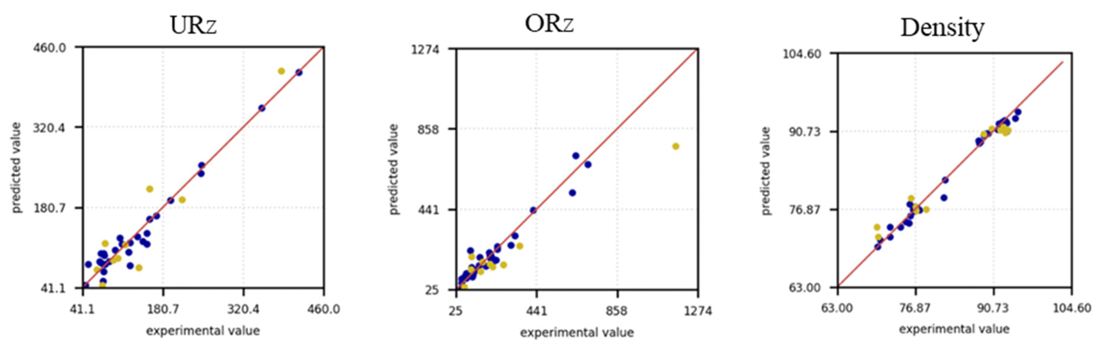
For ORz (Figure 8, center), the model demonstrates superior predictive accuracy for small roughness values (< 441 µm), as evidenced by better alignment with the training data and reduced scatter in the predictions. This indicates that the model effectively captures the underlying patterns within this range, likely due to a higher density of data points or less variability in the observed values. However, as roughness increases beyond this threshold, the accuracy of the predictions deteriorates, accompanied by a noticeable increase in scatter. This decline suggests that the model struggles to generalize to larger roughness values, potentially due to a lack of sufficient data or increased complexity in the relationships governing higher roughness levels. Addressing this issue may require additional data for large roughnesses or the inclusion of features that better capture the variability in this range. The situation is the same for the test data of ORz, although the deviation of the predictions is generally significantly larger. In the density prediction (Figure 8, right), the training data are well adapted to the experimental data and an accurate prediction with few outliers is made for both low and high density values. For the test data, the predictions for low density values tend to be overestimated with a few outliers, while for high density predictions the values are primarily underestimated.

5. Discussion

The initial attempt to utilize and optimize a single ML model for predicting all three parameters —URz, ORz, and Density— was unsuccessful. The primary limitation was the small size of the measurement dataset, coupled with the substantial variability in the parameter values. These factors hindered the model's ability to capture consistent patterns across all targets, ultimately preventing it from providing reliable and usable predictions. Furthermore, the small data set restricts the model's ability to generalize to unseen data and with the limited samples, the risk of overfitting increases, reducing predictive reliability for new process conditions. Additionally, the small datasets may not fully capture the variability in process parameters, leading to biased or unstable model performance. This observation underscores the need for either an increased dataset size, feature-specific models, or tailored preprocessing strategies to better account for the distinct characteristics and variances of each parameter in order to improve model robustness and generalizability. As a result, it became necessary to train and test the models individually for each parameter. The evaluated models LR, RFR, SVM, kNN, MLP, and Bag demonstrated varying levels of performance and robustness during hyperparameter optimization. As anticipated, the LR model failed to achieve a high R² value and a low RMSE due to the complexity of the relationships between input and output variables. The predictions from the LR model exhibited significant deviations from the actual experimental data, indicating that this approach is unsuitable for accurately modeling the investigated parameters. According to [10] it is an indication that conventional regression models cannot solve the problem and that a ML approach is required. This can be attributed to the inherent limitations of LR in capturing complex, non-linear relationships within the data. The MEX/M process involves multiple interacting parameters, such as material properties, process conditions, and geometric features, which exhibit non-linear dependencies. Since LR assumes a linear relationship between the input features and the target variables, it was unable to adequately model the intricate patterns present in the dataset. Consequently, the LR model showed poor generalization performance and was deemed unsuitable for making accurate predictions in this context.

After 10 optimization iterations, the RFR model showed worse results than the MLP and Bag models. A negative value of R² of -1.97 led to exclusion of the model for further investigations. A negative R² value means that the model performs worse than a trivial model that only uses the mean value of the target variable as a prediction. Specifically, the model not only does not explain any variance in the data, but also provides predictions that increase the error variance, which is also observed in [42]. For RFR, the negative R² values may be attributed to over-complexity in the model, such as an excessive number of trees or insufficient regularization during hyperparameter tuning. This caused the model to overfit subtle patterns or noise in the training dataset, which were not representative of the overall data distribution. In both cases, negative R² values highlight that the models performed worse than a simple baseline prediction (e.g., predicting the mean of the target variable). This underscores the importance of carefully balancing model complexity and regularization during hyperparameter optimization to ensure reliable predictions and robust generalization.

The SVM model appears to have difficulties in accurately capturing the variability of the URz and ORz values. The data could be non-linearly separable or have a highly non-linear pattern that the SVM model does not capture effectively. With a small number of data points, SVM may have difficulty making robust predictions as it is highly dependent on the number and quality of support vectors, also observed in [43]. SVM is sensitive to unscaled input data. If the data has not been correctly normalized or standardized, this can affect performance. A similar observation was made in the roughness study of SVM in [44] where the accuracy of 0.56 was also the worst for roughness predictions. This poor performance can be attributed to several factors inherent to the nature of the dataset and the characteristics of the SVM model. Firstly, SVM models, especially when used with non-linear kernels, can struggle with small datasets that have high variability or noise. The limited number of experimental data points in this study likely led to overfitting during training, where the model attempted to fit every detail in the data, including noise. This overfitting reduced the model's ability to generalize to unseen data, resulting in poor test performance. Secondly, the high dimensionality or complex feature interactions in the dataset may have exacerbated the model's inability to find an optimal decision boundary. SVM requires careful tuning of hyperparameters such as the regularization parameter C and the kernel-specific parameters (e.g., gamma for the RBF kernel). Without sufficient data to guide this tuning process effectively, the model's performance likely deteriorated further. Lastly, SVMs are sensitive to feature scaling and may fail to perform well if input features are not properly normalized. Given these challenges, SVM was unable to capture the intricate relationships in the dataset, resulting in poor predictive accuracy and high error rates, making it the least effective model for this application.

For the kNN model, a negative R² factor also appeared in the test for URz after 10 trainings. In addition, a value of 1 and an RMSE of 0 occurred in the training for the R² value of ORz. A negative R² value indicates that the kNN model's predictions are worse than a simple baseline model. This suggests that the model fails to capture the patterns in the test data, which may be due to overfitting to the training data. A R² value of 1 and 0 RMSE indicate that the kNN model memorized the training data perfectly for ORz. While this may seem ideal, it often signals overfitting, where the model performs exceptionally well on the training data but struggles to generalize to unseen test data. This issue arises because the kNN algorithm stores the training dataset and bases predictions on the closest neighbors. If k is too small (e.g., k=1), the model essentially memorizes the training points, making it sensitive to noise and unable to generalize well to unseen data. This behavior indicates that the models were overfitting the training data, leading to a significant loss of generalization ability. For kNN, this issue likely arose from an inappropriate selection of the number of neighbors (k). Therefore, the kNN model was not considered further for parameter optimization.

The experimentally measured surface roughnesses are significantly higher than the roughness values found in the literature due to the overhang angle [45,46,47]. As shown in [45], the process parameters have a significant influence on the surface roughness of the components. A comparison with the recorded measurement data show that the geometry of the inclined walls has a much greater influence (factor 10) than the parameter variations. The measured values, which act as a data set for the ML models, also vary considerably. For URz, the variance in the measurement data is notably lower compared to ORz, which facilitates more effective training and hyperparameter optimization. The reduced variability allows the model to capture the underlying patterns more reliably, leading to improved predictive accuracy. After 50 iterations of hyperparameter optimization, the predictions for URz exhibit higher precision and better alignment with experimental values compared to ORz. This suggests that the lower variance in the measurement data for URz not only enhances model training but also contributes to improved generalization performance. In contrast, the higher variance observed in ORz data likely introduces additional challenges in modeling and optimization, resulting in less accurate predictions.

The average accuracy of the predictions is defined as:

$$Averageaccuracy=1-{\displaystyle \frac{RMSE}{\sum _1^n{R}_{z_n}}}$$

(1)

The accuracy in the test data set for URz is 75.71 %, which makes a prediction possible. For ORz, the average accuracy is only 39.26 % and an exact prediction is not generally feasible. The MLP model performed more accurately for the prediction of URz than for ORz based on the evaluation criteria examined and the predictions of test and training data. The representativeness and size of the training dataset are critical for the model's ability to generalize to new data [48]. Since the ORz data is highly variable and there is only a small amount of data, an accurate prediction is difficult and requires the input of more data. In addition, even after 50 training sessions, the standard deviation of 20.47 µm in the test case is a power of ten higher than for URz and a prediction is inadmissible. Larger roughness values may be associated with increased complexity or variability in the underlying physical processes such as the stair case effect [49,50], making them harder to predict accurately.

The density of the sample geometries was experimentally determined to range between 70 % and 95 % using the Archimedes method. While this does not meet the typical standards for Metal Injection Molding (MIM), it falls within the empirically established density range for the Material Extrusion for Metals (MEX/M) process, as reported in the literature [22]. This suggests that the density values observed are consistent with the inherent characteristics of the MEX/M process, which is known to result in slightly lower densities compared to MIM due to differences in processing parameters and material behavior. The average accuracy of the density predictions in the test dataset using the Bag model, calculated according to Equation (1), is 97.44%. This indicates that the model provides highly accurate predictions within the same order of magnitude as the experimental data. The deviation of only 1.55% compared to the accuracy of [4] for the density prediction underscores the reliability of the model in capturing the underlying patterns of the dataset. Such a small deviation highlights the model's robustness and suitability for predicting density in similar experimental setups.

6. Conclusions

For the MEX/M process, the upskin and downskin surface roughness, along with the density, were empirically determined as experimental values for various overhang angles. These measurements provide critical insights into the relationship between geometric features and resulting material properties, which are essential for optimizing process parameters and achieving desired part characteristics in MEX/M applications. The experimental data served as the foundation for predicting the upskin and downskin surface roughness, as well as the density of MEX/M samples. To achieve this, machine learning models, including LR, RFR, SVM, kNN, MLP, and Bag, were trained on the dataset. The performance of these models was evaluated using the R² coefficient and RMSE as metrics. Additionally, prediction plots were analyzed to assess the accuracy and reliability of the models in capturing the relationships between experimental variables and target properties. The following findings were obtained from the investigations:

• The LR model proved to be unsuitable for predicting the upskin and downskin roughness, as well as the density, due to its low R² values and high RMSE in both training and testing phases.
• The SVM model exhibited the lowest R² value and the highest RMSE among all evaluated models, making it even less suitable than the LR model for predicting the upskin and downskin roughness of MEX/M samples.
• The kNN and RFR models demonstrated greater robustness compared to LR, achieving relatively higher R² values and lower RMSE during initial evaluations. However, after several iterations of hyperparameter optimization, both models exhibited negative R² values for certain target variables, particularly in the test phase.
• The MLP model was identified as a strong candidate for predicting the surface roughness (upskin and downskin) in MEX/M samples. Its suitability stems from its ability to handle complex, non-linear relationships within the data, which are characteristic of the MEX/M process. The MLP model's architecture, consisting of interconnected layers of neurons, enables it to capture intricate patterns and interactions among the input features, making it well-suited for modeling the variability in surface roughness. Moreover, through proper hyperparameter optimization, including the adjustment of the number of hidden layers, neurons, activation functions, and learning rates, the MLP achieved high R² values and low RMSE, demonstrating its robustness and accuracy in both training and test datasets for URz. Furthermore, an average accuracy of only 39 % is too imprecise, so that no predictions can be made for ORz with the current data set.
• The Bag model was identified as a suitable approach for predicting the density of MEX/M samples, achieving an average prediction accuracy of 97.44%. This high level of accuracy can be attributed to the ensemble nature of the Bagging method, which combines multiple base models to reduce variance and improve robustness.
• An attempt to predict both surface roughness and density within a single model for different stages of the process chain was not feasible. This limitation can be attributed to the fundamentally different nature of the target variables and the complex interactions between process parameters at various stages.
• Overall, the failure of regression models underscores the necessity of employing more experimental data and eventually advanced machine learning approaches, such as ensemble methods or neural networks, which are better equipped to handle non-linear relationships and complex data structures inherent in additive manufacturing processes.

The results demonstrate that the choice of model and its hyperparameter optimization significantly influence the predictive accuracy for MEX/M sample properties, providing a robust framework for future process optimization and design improvements. With the aid of ML models, it is possible in future to reduce intensive experimental test series and efficiently find suitable material properties.

References

- ISO/ASTM 52900:2023 - Additive manufacturing — General principles - Part positioning, coordinates and orientation, (2023).
- Kuehne, M.; Bartsch, K.; Bossen, B.; Emmelmann, C. , Predicting melt track geometry and part density in laser powder bed fusion of metals using machine learning, Prog. Addit. Manuf. 2023, 8, 47–54. [Google Scholar] [CrossRef]
- Bartsch, K. , Digitalization of design for support structures in laser powder bed fusion of metals, Springer Nature Switzerland, Cham, 2023. [CrossRef]
- Bossen, B.; Kuehne, M.; Kristanovski, O.; Emmelmann, C. , Data-driven density prediction of AlSi10Mg parts produced by laser powder bed fusion using machine learning and finite element simulation, J. Laser Appl. 2023. [CrossRef]
- Gor, M.; Dobriyal, A.; Wankhede, V.; Sahlot, P.; Grzelak, K.; Kluczyński, J.; Łuszczek, J. , Density Prediction in Powder Bed Fusion Additive Manufacturing: Machine Learning-Based Techniques, Appl. Sci. 2022, 12, 7271. [Google Scholar] [CrossRef]
- Kumar, S.; Gopi, T.; Harikeerthana, N.; Gupta, M.K.; Gaur, V.; Krolczyk, G.M.; Wu, C. , Machine learning techniques in additive manufacturing: a state of the art review on design, processes and production control, J. Intell. Manuf. 2023, 34, 21–55. [Google Scholar] [CrossRef]
- Bossen, B.; Kuehne, M.; Kristanovski, O.; Emmelmann, C. , Data-driven density prediction of AlSi10Mg parts produced by laser powder bed fusion using machine learning and finite element simulation, J. Laser Appl. 2023, 35, 042023. [Google Scholar] [CrossRef]
- Wischeropp, T.M.; Tarhini, H.; Emmelmann, C. , Influence of laser beam profile on the selective laser melting process of AlSi10Mg, J. Laser Appl. 2020, 32, 022059. [Google Scholar] [CrossRef]
- Wu, D.; Wei, Y.; Terpenny, J. , Predictive modelling of surface roughness in fused deposition modelling using data fusion, Int. J. Prod. Res. 2019, 57, 3992–4006. [Google Scholar] [CrossRef]
- Asami, K.; Roth, S.; Krukenberg, M.; Röver, T.; Herzog, D.; Emmelmann, C. , Predictive modeling of lattice structure design for 316L stainless steel using machine learning in the L-PBF process, J. Laser Appl. 2023, 35, 042046. [Google Scholar] [CrossRef]
- Sivakumar, N.K.; Palaniyappan, S.; Bodaghi, M.; Azeem, P.M.; Nandhakumar, G.S.; Basavarajappa, S.; Pandiaraj, S.; Hashem, M.I. , Predictive modeling of compressive strength for additively manufactured PEEK spinal fusion cages using machine learning techniques, Mater. Today Commun. 2024, 38, 108307. [Google Scholar] [CrossRef]
- Wang, H.; Al Shraida, H.; Jin, Y. , Predictive modeling for online in-plane shape deviation inspection and compensation of additive manufacturing, Rapid Prototyp. J. 2024, 30, 350–363. [Google Scholar] [CrossRef]
- Rodríguez-Martín, M.; Fueyo, J.G.; Gonzalez-Aguilera, D.; Madruga, F.J.; García-Martín, R.; Muñóz, Á.L.; Pisonero, J. , Predictive Models for the Characterization of Internal Defects in Additive Materials from Active Thermography Sequences Supported by Machine Learning Methods, Sensors 2020, 20, 3982. [CrossRef]
- Sarkon, G.K.; Safaei, B.; Kenevisi, M.S.; Arman, S.; Zeeshan, Q. , State-of-the-Art Review of Machine Learning Applications in Additive Manufacturing; from Design to Manufacturing and Property Control, Arch. Comput. Methods Eng. 2022, 29, 5663–5721. [Google Scholar] [CrossRef]
- Zhang, Y.; Safdar, M.; Xie, J.; Li, J.; Sage, M.; Zhao, Y.F. , A systematic review on data of additive manufacturing for machine learning applications: the data quality, type, preprocessing, and management, J. Intell. Manuf. 2023, 34, 3305–3340. [Google Scholar] [CrossRef]
- Mahmoud, D.; Magolon, M.; Boer, J.; Elbestawi, M.A.; Mohammadi, M.G. , Applications of Machine Learning in Process Monitoring and Controls of L-PBF Additive Manufacturing: A Review, Appl. Sci. 2021, 11, 11910. [Google Scholar] [CrossRef]
- Razvi, S.S.; Feng, S.; Narayanan, A.; Lee, Y.-T.T.; Witherell, P. , A Review of Machine Learning Applications in Additive Manufacturing, in: Vol. 1 39th Comput. Inf. Eng. Conf., American Society of Mechanical Engineers, Anaheim, California, USA, 2019: p. V001T02A040. [CrossRef]
- Babu, S.S.; Mourad, A.-H.I.; Harib, K.H.; Vijayavenkataraman, S. , Recent developments in the application of machine-learning towards accelerated predictive multiscale design and additive manufacturing, Virtual Phys. Prototyp. 2023, 18, e2141653. [Google Scholar] [CrossRef]
- Gaikwad, M.U.; Gaikwad, P.U.; Ambhore, N.; Sharma, A.; Bhosale, S.S. , Powder Bed Additive Manufacturing Using Machine Learning Algorithms for Multidisciplinary Applications: A Review and Outlook, Recent Pat. Mech. Eng. 2025, 18, 12–25. [Google Scholar] [CrossRef]
- Jyeniskhan, N.; Keutayeva, A.; Kazbek, G.; Ali, M.H.; Shehab, E. , Integrating Machine Learning Model and Digital Twin System for Additive Manufacturing, IEEE Access 2023, 11, 71113–71126. [CrossRef]
- Yao, X.; Moon, S.K.; Bi, G. , A hybrid machine learning approach for additive manufacturing design feature recommendation, Rapid Prototyp. J. 2017, 23, 983–997. [Google Scholar] [CrossRef]
- Suwanpreecha, C.; Manonukul, A. , A Review on Material Extrusion Additive Manufacturing of Metal and How It Compares with Metal Injection Moulding, Metals 2022, 12, 429. [CrossRef]
- Herzog, D.; Asami, K.; Scholl, C.; Ohle, C.; Emmelmann, C.; Sharma, A.; Markovic, N.; Harris, A. , Design guidelines for laser powder bed fusion in Inconel 718, J. Laser Appl. 2022, 34, 012015. [Google Scholar] [CrossRef]
- Asami, M.K.; Herzog, D.; Bossen, B.; Geyer, L.; Klemp, C.; Emmelmann, C. , Design Guidelines For Green Parts Manufactured With Stainless Steel In The Filament Based Material Extrusion Process For Metals (MEX/M), (2022). [CrossRef]
- Asami, K.; Lozares, J.M.C.; Ullah, A.; Bossen, B.; Clague, L.; Emmelmann, C. , Material extrusion of metals: Enabling multi-material alloys in additive manufacturing, Mater. Today Commun. 2024, 38, 107889. [Google Scholar] [CrossRef]
- Pedregosa, F.; Varoquaux, G.; Gramfort, A.; Michel, V.; Thirion, B.; Grisel, O.; Blondel, M.; Prettenhofer, P.; Weiss, R.; Dubourg, V.; Vanderplas, J.; Passos, A.; Cournapeau, D.; Brucher, M.; Perrot, M.; Duchesnay, É. , Scikit-learn: Machine Learning in Python, J. Mach. Learn. Res. 2011, 12, 2825–2830. [Google Scholar]
- Asami, M.K.; Kuehne, M. , Machine Learning Models and Data for the Application of Machine Learning in Predicting Quality Parameters in Metal Material Extrusion (MEX/M), (2025). [CrossRef]
- Othman, W.; Hamoud, B.; Kashevnik, A.; Shilov, N.; Ali, A. , A Machine Learning-Based Correlation Analysis between Driver Behaviour and Vital Signs: Approach and Case Study, Sensors 2023, 23, 7387. [CrossRef]
- Huang, J.; Wei, Y. , Data-driven analysis of stroke-related factors and diagnostic prediction, in: 2024 IEEE 6th Adv. Inf. Manag. Commun. Electron. Autom. Control Conf. IMCEC, IEEE, Chongqing, China, 2024: pp. 60–65. [CrossRef]
- Rezazadeh, A. , Toe-Heal-Air-Injection Thermal Recovery Production Prediction and Modelling Using Quadratic Poisson Polynomial Regression., ArXiv Signal Process. (2020). https://api.semanticscholar.org/CorpusID:227305649.
- Géron, A. , Hands-on machine learning with Scikit-Learn, Keras, and TensorFlow: concepts, tools, and techniques to build intelligent systems, Second edition, O’Reilly, Beijing Boston Farnham Sebastopol Tokyo, 2019.
- Xiao, W.; Wang, Y. , The Application of Partially Functional Linear Regression Model in Health Science, Sci. Discov. 2020, 8, 134. [Google Scholar] [CrossRef]
- Roy, M.-H.; Larocque, D. , Robustness of random forests for regression, J. Nonparametric Stat. 2012, 24, 993–1006. [Google Scholar] [CrossRef]
- Adankon, M.M.; Cheriet, M. Support Vector Machine, in: S.Z. Li, A.K. Jain (Eds.), Encycl. Biom., Springer US, Boston, MA, 2015: pp. 1504–1511. [CrossRef]
- Rachdi, M.; Laksaci, A.; Kaid, Z.; Benchiha, A.; Al-Awadhi, F.A. , k -Nearest neighbors local linear regression for functional and missing data at random, Stat. Neerlandica 2021, 75, 42–65. [Google Scholar] [CrossRef]
- Kramer, A. , Dimensionality Reduction by Unsupervised K-Nearest Neighbor Regression, in: 2011 10th Int. Conf. Mach. Learn. Appl. Workshop, IEEE, Honolulu, HI, USA, 2011: pp. 275–278. [CrossRef]
- S.-T. Bow, ed., Multilayer Perceptron, in: Pattern Recognit. Image Preprocessing, CRC Press, 2002: pp. 201–224. [CrossRef]
- Taud, H.; Mas, J.F.; Perceptron, M.; Olmedo, M.T.C.; Paegelow, M.; Mas, J.-F.; Escobar, F.; Scenar, G.A.M.L.C.; Publishing, S.I. ; Cham, 2018: pp. 451–455. [CrossRef]
- Hassan, H.A.; Ghani, M.N.A.A.; Zabidi, A.; Adnan, W.N.W.M.; Rahman, J.A.; Rusni, I.M. , Pattern Classification in Recognising Idgham Maal Ghunnah Pronunciation Using Multilayer Perceptrons, in: 2024 IEEE 6th Symp. Comput. Amp Inform. ISCI, IEEE, Kuala Lumpur, Malaysia, 2024: pp. 333–338. [CrossRef]
- Meng, L.; McWilliams, B.; Jarosinski, W.; Park, H.-Y.; Jung, Y.-G.; Lee, J.; Zhang, J. , Machine Learning in Additive Manufacturing: A Review, JOM 2020, 72, 2363–2377. [CrossRef]
- Chicco, D.; Warrens, M.J.; Jurman, G. , The coefficient of determination R-squared is more informative than SMAPE, MAE, MAPE, MSE and RMSE in regression analysis evaluation, PeerJ Comput. Sci. 2021, 7, e623. [Google Scholar] [CrossRef]
- Klusowski, J.M. , Sharp Analysis of a Simple Model for Random Forests, (2020). [CrossRef]
- Battineni, G.; Chintalapudi, N.; Amenta, F. , Machine learning in medicine: Performance calculation of dementia prediction by support vector machines (SVM), Inform. Med. Unlocked 2019, 16, 100200. [Google Scholar] [CrossRef]
- Toorandaz, S.; Taherkhani, K.; Liravi, F.; Toyserkani, E. , A novel machine learning-based approach for in-situ surface roughness prediction in laser powder-bed fusion, Addit. Manuf. 2024, 91, 104354. [Google Scholar] [CrossRef]
- Caminero, M.Á.; Gutiérrez, A.R.; Chacón, J.M.; García-Plaza, E.; Núñez, P.J. , Effects of fused filament fabrication parameters on the manufacturing of 316L stainless-steel components: geometric and mechanical properties, Rapid Prototyp. J. 2022, 28, 2004–2026. [Google Scholar] [CrossRef]
- Gloeckle, A.; Konkol, T.; Jacobs, O.; Limberg, W.; Ebel, T.; Handge, U.A. , Processing of Highly Filled Polymer–Metal Feedstocks for Fused Filament Fabrication and the Production of Metallic Implants, Materials 2020, 13, 4413. [CrossRef]
- Damon, J.; Dietrich, S.; Gorantla, S.; Popp, U.; Okolo, B.; Schulze, V. , Process porosity and mechanical performance of fused filament fabricated 316L stainless steel, Rapid Prototyp. J. 2019, 25, 1319–1327. [Google Scholar] [CrossRef]
- Siamidoudaran, M.; İşçioğlu, E. , Injury Severity Prediction of Traffic Collision by Applying a Series of Neural Networks: The City of London Case Study, PROMET - TrafficTransportation 2019, 31, 643–654. [CrossRef]
- Eyerci, Ö.; Aladağ, M. , NON-PLANAR TOOLPATH FOR LARGE SCALE ADDITIVE MANUFACTURING, Int. J. 3D Print. Technol. Digit. Ind. 2021, 5, 477–487. [Google Scholar] [CrossRef]
- Rajput, A.S.; Babu, P.; Das, M.; Kapil, S. , Influence of toolpath strategies during laser polishing on additively manufactured biomaterials, Surf. Eng. 2024, 40, 967–982. [Google Scholar] [CrossRef]
Disclaimer/Publisher’s Note: The statements, opinions and data contained in all publications are solely those of the individual author(s) and contributor(s) and not of MDPI and/or the editor(s). MDPI and/or the editor(s) disclaim responsibility for any injury to people or property resulting from any ideas, methods, instructions or products referred to in the content. |
© 2025 by the authors. Licensee MDPI, Basel, Switzerland. This article is an open access article distributed under the terms and conditions of the Creative Commons Attribution (CC BY) license (https://creativecommons.org/licenses/by/4.0/).
Copyright: This open access article is published under a Creative Commons CC BY 4.0 license, which permit the free download, distribution, and reuse, provided that the author and preprint are cited in any reuse.