Submitted:
09 February 2026
Posted:
11 February 2026
You are already at the latest version
Abstract
Heating gases to high temperatures is essential for supplying energy to thermal and thermochemical processes. This study presents the optical–thermal design of a mini heliostat field coupled with a tubular solar receiver equipped with second optics, aiming to heat nitrogen to approximately 850 K. The secondary optical system redistributed up to 40% of the incident solar flux from the front to the rear surface of the receiver, improving radial temperature uniformity and significantly reducing thermal gradients along the tube wall. An overall optical efficiency of 65.25% was achieved, accounting for atmospheric attenuation, shading, blocking, and the cosine effect. A coupled computational model was developed by solving the conservation equations of mass, momentum, and energy, with the spatially resolved solar flux distribution obtained via ray tracing used as a thermal boundary condition. The simulation results, validated with an empirical correlation, include solar flux contours, nitrogen temperature distributions, surface temperatures, and heat transfer coefficients. The configuration with a 12 mm vertex spacing between secondary reflectors demonstrated the best thermal performance, reducing the maximum tube surface temperature by 11% and improving radial symmetry, while maintaining nitrogen outlet temperatures near the design target of 850 K. These results confirm the suitability of the system for high-temperature applications such as solar pyrolysis using nitrogen as the heat transfer fluid to deliver the required thermal energy.
Keywords:
optical-thermal analysis
; second optics
; solar receivers
; solar tower system
; gas heating
1. Introduction
Fossil fuels currently supply approximately 80% of global energy [1], contributing to significant environmental issues, including climate change. To address this, renewable energy technologies have emerged as sustainable alternatives. Among these, concentrated solar power (CSP) systems harness sunlight by converting solar radiation into heat to elevate the temperature of a moving fluid within a thermal receiver [2]. The primary CSP configurations include central tower, parabolic trough, linear Fresnel, and dish-Stirling systems. Research indicates that solar tower technology is particularly effective for generating thermal energy exceeding 700 °C, making it suitable for numerous industrial applications.
A central tower system comprises key components: a heliostat field, a central tower, and a receiver. Heliostats direct sunlight toward the receiver atop the tower [3], transferring concentrated solar energy to the heat transfer fluid (HTF). Solar receivers can be categorized by operating pressure, HTF type, andtructural design [4].
Gas-phase receivers are considered one of the most promising near-term solutions for high-temperature applications due to their inert behavior at elevated temperatures and greater reliability compared to liquid or solid heat transfer materials (HTMs) [5]. Additionally, they pose minimal environmental risks and could offer cost advantages. However, gaseous heat transfer fluids (HTFs) have inherent drawbacks, including low thermal efficiency and poor heat transfer properties [5,6]. To address these limitations, various gas-phase receiver designs have been developed, primarily focusing on enhancing heat transfer between the solar absorber and the HTF [7,8]. A key challenge with gas-phase receivers is their exposure to non-uniform solar flux, which is highly concentrated on the tube surfaces. This can create large temperature gradients between the front and back of the receiver tubes, leading to thermal stress and deformation. These issues can be significantly mitigated by using second optics to evenly distribute radiation across the entire tube surface and by optimizing the heliostat field layout.
Among the various inert gases employed in high-temperature solar processes, recent reviews of solar pyrolysis systems [9] report that approximately 46% of projects use nitrogen, while 47% use argon as the inert atmosphere[10]. In this study, nitrogen was selected as the heat transfer fluid (HTF) not only because of its availability and lower cost compared to argon, but also because it continues our research group’s previous work on solar-driven thermochemical conversion systems [11,12].
Next, the literature survey has been categorized into three topics: (a) methodologies for heliostat field design, (b) use of second optics to improve solar flux distribution in the thermal receiver of different solar concentration technologies, and (c) heating of gases with tubular receivers of solar tower technology.
1.1. Methodologies for Heliostat Field Design
Sánchez and Romero [13] introduced a methodology for designing heliostat field layouts using annual normalized energy surfaces. Later, Besarati and Goswami [14] proposed a simplified approach to identify heliostats most affected by shadowing and blocking, reducing computational time while maintaining accuracy compared to existing literature. Barberena et al. [15] conducted a comprehensive review of heliostat field layout algorithms and concluded that different methods yield comparable solar field efficiencies.
Zhang et al. [16] developed an enhanced code integrating flat mapping and ray tracing techniqu and compared radial staggered and biomimetic spiral layouts. Their findings indicated that the spiral configuration outperformed the radial layout in northern fields. Srilakshmi et al. [17] proposed a performance estimation method for tower plants with external cylindrical receivers, validating their approach using data from Spain’s Gemasolar and the U.S.’s Crescent Dunes plants.
Further advancements were made by Raj and Bhattacharya [18], who introduced an improved methodology for assessing shading and blocking efficiency. Their approach achieved ray-tracing-level accuracy with fewer computational grid points. Haris et al. [19] compared radial staggered and Fermat’s spiral layouts, optimizing by using a rejection-sampling-based Genetic Algorithm (GA). The spiral configuration demonstrated a 14.62% increase in annual efficiency. Most recently, Biencinto et al. [20] presented HEFESTO, a novel software for preliminary heliostat field design. Validation against real-world data from the CESA-I field and ray-tracing simulations confirmed their high accuracy.
1.2. Use of Second Optics to Improve Solar Flux Distribution in Thermal Receivers
Sookramoon [21] designed, constructed, and evaluated a two-stage parabolic trough concentrator (PT featuring a polished stainless-steel primary reflector and a multi-piece hyperbolic secondary mirror. The system used a glass-covered, blackened copper pipe as the receiver, achieving a peak thermal efficiency of 23.43%, an optical efficiency of 76%, and a geometric concentration ratio of 27.08X. Widyolar et al. [22] later developed a hybrid photovoltaic/solar power system combining a parabolic trough with a compound parabolic secondary, reaching 50X concentration and 600 °C operation using alumina-based particulate fluid. Their prototype attained 63% optical efficiency and 4% net solar-to-electric efficiency in the PV subsystem.
Bharti et al. [23] analyzed receiver misalignment and secondary reflector designs, comparing parabolic (PSR) and triangular (TSR) secondaries against a no-reflector (WSR) configuration. The PSR achieved the highest thermal efficiency (24.3%) and had more uniform receiver tube temperatures than the WSR. Maatallah and Ammar [24] introduced a homogenizing reflector (HR) to mitigate thermal stress from flux non-uniformity in PTCs. While optical efficiency dropped by 7%, flux uniformity improved drastically, reducing peak flux gradients from 80 to 11 kW/m².
Gong et al. (2020) [25] enhanced large-aperture PTCs using an adaptive secondary reflector (SR) composed of multiple parabolas, boosting optical and thermal efficiency by 5.2% and 4.9%, respectively, while doubling flux uniformity. Tang et al. [26] proposed a segmented broken-line SR design that balances upper- and lower-absorber flux via optimized positioning. Their design achieved >90% flux uniformity and an optical efficiency higher than that of existing SRs.
Mandal et al. [27] modeled a hyperbolic cavity receiver with secondary reflection for dish concentrators, achieving 91.72% efficiency at optimal geometry (h₁=0.75 m, d/h=0.5). Rodriguez-Sanchez and Rosengarten [28] used ray-tracing to show that truncated flat secondaries reduce shading effects, increasing concentration by 20–80% with minimal efficiency losses (<3.5%).
1.3. Heating Gases with Tubular Receivers of Solar Tower Technology
1.3.1. Nitrogen
Maytorena et al. [11] proposed an innovative system for the fast pyrolysis of biomass using concentrated solar energy. This system employs a field of biomimetically arranged mini-heliostats and an external tubular thermal receiver to heat nitrogen. Nitrogen is used as a heat-transfer medium in a fluidized-bed pyrolysis reactor. The results demonstrate that the system can achieve high temperatures, significantly improving the quality of the biofuel produced and offering a sustainable alternative to conventional methods.
1.3.2. Air
Quero et al. [29] and Korzynietz et al. [30] presented the Solugas project, the first large-scale hybrid solar plant integrating a solarized gas turbine. The study analyzed the performance of key components, such as the solar pressurized air receiver and the gas turbine, demonstrating the high potential of this technology for solar thermal electricity generation. They concluded that, although the technology is promising, challenges remain in incorporating solar heat at high temperatures and integrating combined cycles to achieve higher efficiency. Cantone et al. [31] investigated the thermal behavior of three absorber tubes, both smooth and with turbulence promoters (annular and helical rings), subjected to unilateral heating. The experimental results show that turbulence promoters significantly reduce the maximum wall temperature in the tube, thereby smoothing the thermal gradients generated by unilateral heating. The validated CFD models found that tubes with turbulence promoters exhibit better thermal performance and lower thermal stress. Bashir et al. [32] investigated the effect of geometry on the performance of solar receivers integrated with phase change materials (PCM) in solar dish-powered microturbine systems. Using Ansys Fluent numerical simulations, they evaluated three tube arrangements and two cavity structures. The results showed that the receiver with a conical cavity and 172° tubes offers a more uniform temperature distribution and more homogeneous PCM solidification.
Rednic et al. [33] designed and optimized a high-temperature solar receiver to enhance the efficiency of CSP systems. Using numerical simulations and experimental evaluations, the study demonstrates that the optimized receiver design can achieve thermal efficiencies exceeding 80% and a uniform temperature distribution, both of which are crucial for preventing material damage and extending the receiver’s lifespan. Shuai et al. [34] presented a hybrid model that combines numerical simulations and deep learning to optimize tubular solar receivers in CSP systems. The results showed maximum efficiencies of 48.9%, 53.2%, and 56.8% for flow rates of 0.5, 0.75, and 1 kg/s, respectively, and a maximum thermal efficiency of 89.8% in heating systems. Additionally, the proposed optimization strategy significantly reduces the maximum wall temperature of the receiver tube. Kadohiro et al. [35] investigated tubular cavity solar receivers using helical tubes to generate superheated steam and hot air simultaneously. The research focused on the thermal and exergy efficiencies of different receiver configurations. The results showed that the receiver with cylindrical and conical helical tubes exhibited the highest thermal efficiency (67.0%) and exergy efficiency (46.9%).
1.3.3. Air with Supercritical Carbon Dioxide
Zheng et al. [36] presented a comprehensive analysis of the performance of different heat transfer fluids in tubular receivers for concentrating solar tower systems. Using energy and exergy analysis, they compare fluids such as molten salt, liquid sodium, supercritical carbon dioxide (sCO2), air, and water/steam. They highlighted that systems operating with sCO2 and air, although promising in other CSP applications, are not suitable for simple tubular receivers due to high pressure stresses and external heat losses. Additionally, the researchers found that air-operated receivers perform better than those using sCO2 in terms of pressure stresses and heat losses.
1.3.4. Supercritical Carbon Dioxide (sCO2)
Montes et al. [37,38] introduced a microchannel-based central receiver with radially arranged vertical panels, optimized for pressurized gases and sCO₂. Their design enhanced exergy efficiency by balancing heat loss, pressure drop, and optical performance. Chen et al. [39] evaluated a conical sCO₂ receiver with an internal helical tube, identifying optimal performance at an aspect ratio of 1.5 and angle ratio of 0.25, achieving 85.67% thermal efficiency (though with elevated thermal stress in upward flow configurations) Fernandez-Torrijos et al. [40] performed a thermo-mechanical and economic assessment of tubular sCO₂ receivers, demonstrating that smaller tubes maximize plant efficiency and reduce costs while ensuring a 25-year operational lifespan.
Wang et al. (2024) [41] conducted a three-dimensional optimization of fins for compact solar receivers using supercritical CO₂ (sCO₂). Their design featured fins with variable cross-sections along their height, significantly improving thermal efficiency while minimizing entropy generation. Similarly, Fronk et al. [42] developed a modular solar receiver with a micro-pin array capable of operating at temperatures above 700 °C and pressures up to 20 MPa. Experimental tests demonstrated thermal efficiencies exceeding 90% and robust performance under repeated pressure cycling. Zhang et al. [43]analyzed convective heat transfer in serpentine sCO₂ receiver tubes under non-uniform flow and low Reynolds numbers. The serpentine design improved heat transfer by 23% and reduced entropy generation by 22% compared to conventional straight tubes. Pérez-Álvarez et al. [44] explored bimetallic receiver tubes for solar tower plants, finding that three-layer tubes—incorporating a high-thermal-conductivity intermediate material—improved temperature uniformity and reduced thermal stress, extending receiver lifespan.
Despite the promising potential of solar tower systems for high-temperature applications, the highly localized solar flux typically concentrated on the front surfaces of tubular receivers often results in high radial thermal gradients and mechanical stresses, compromising system durability. Although several optical designs have been proposed for central receivers, there is limited research specifically addressing the use of second optics in solar tower systems for gas-phase heating at high temperatures. This limitation is particularly relevant for thermochemical processes, such as pyrolysis, which demand uniform and stable temperature profiles along the receiver walls. In response to this gap, the present study proposes and evaluates a coupled optical–thermal computational model to assess the effect of integrating a secondary optical system into a mini heliostat field configuration. The receiver is designed to heat nitrogen (selected for its inertness, availability, and relevance to pyrolysis research) to approximately 850 K. The model incorporates the detailed solar flux distribution obtained through ray-tracing simulations as a thermal boundary condition and solves the governing equations of mass, momentum, and energy conservation. This approach allows us to quantify the impact of second optics on flux redistribution, temperature uniformity, thermal symmetry, and outlet gas temperature, ultimately improving the performance and structural reliability of the receiver. The simulation results are compared with an existing correlation model from the literature to validate the proposed methodology. This comparison confirms the robustness of the CFD model for its intended application in high-temperature environments.
2. Description of the Physical Problem
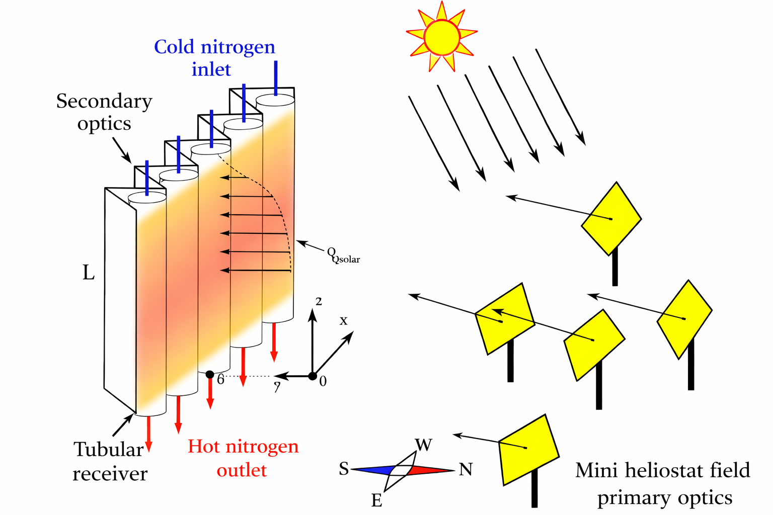
The studied system is shown in Figure 1. It consists of two subsystems: (a) A tubular thermal receiver and (b) A mini-heliostat field. The thermal receiver is used to heat nitrogen to 850 K for thermal or thermochemical applications.
A North-facing heliostat field was developed for Hermosillo, Sonora, Mexico (LAT: 29° 04’ 52’’, LON: -110° 57’ 47’’). Initially, a large field of flat, square heliostats with dimensions of 1.43 × 1.43 meters was considered. Subsequently, they were ordered from most to least power-efficient using an in-house algorithm that performs multiple ray-tracing simulations, developed with the Tonatiuh Script software [45], as explained in the methodology section.
Using an iterative algorithm of ray-tracing coupled (IARCC) with computational fluid dynamics (CFD), the first 170 heliostats were necessary to reach the desired temperature at the outlet of the receiver, encompassing the red and purple heliostats inside the outer polygon in Figure 2 (the polygon has a total area of 1001.3 m²). However, thermal simulations showed that the high incident flux on the receiver tube’s front surface led to high temperature gradients. To reduce temperature gradients, a second optic was implemented to redistribute the 40% of the incident flux from the front to the rear of the thermal receiver. Consequently, using the IARCC, the required number of heliostats was reduced to 119 (red), with a total area of 661.5 m² inscribed within the inner polygon of Figure 2. The total reflect surface is 243.34 m². The receiver’s center is 8.5 m above the surface of the heliostats at position (0, 0, 1), with dimensions of 2 m high by 2 m wide.
The receiver is 2 m wide by 2 m long and has 76 identical tubes for the receiver without second optics (WSO), whereas 54 tubes were considered for the receiver with second optics. Each tube is 2 meters long (L), with an outside diameter (Do) of 25.4 mm and a wall thickness of 2.2 mm (Figure 3). The tube was made of HAYNES® 230 alloy [12], which has the following thermophysical properties: ρ = 8,970 kg/m3, Cp = 473 J/kg K, and k = 18.4 W/m K. The receiving system is directly irradiated at the front with a concentrated solar flux from the mini-heliostat field, while the posterior area of the tubes is irradiated with the second optics concentrator. The considered separation between tubes (s) was 0.0113792 m, and the distance between the tube’s center (C) was 0.0367792 m. The vertex position (V) of the second reflector was varied during the present study. The ends of the second reflector, which are conic, are denoted V1 and V2, and are in the middle of adjacent tubes. The initial value of V is at y’=0.0176 mm, where SO is tangential to the tube.
Nitrogen was considered a thermal fluid, which is an inert species. Nitrogen enters the top of the receiver with a mass flow rate of 0.0071 kg/s at 300 K and leaves the bottom at its maximum temperature (850 K) and a pressure of 1 atm. The nitrogen was considered as an ideal gas for the density (ρ) calculation, and the values of specific heat (Cp), thermal conductivity (k), and viscosity (µ) were considered variable as a function of temperature. Addditionally, a reflectivity of 88% was assumed for the second optics material.
3. Mathematical Models
3.1. Optical Model of the Mini Heliostat Field
The heliostat field distribution was generated using polar coordinates (rⱼ,θⱼ) for each heliostat j, determined by the following equations [50]:
where (rj, θj) is the polar coordinate of the heliostat j, and φ is the golden ratio computed by (1+√5)/2. The index j is the consecutive number of heliostats. In equation (2), a and b are the proportional and exponential factors, and were taken as 0.75 and 0.6, respectively. The atmospheric attenuation efficiency(ηaa) [50] was modeled as a reflectivity modifier based on the receiver’s focal distance (drec) using:
The field’s optical efficiency (η) was computed as the ratio of received to incident power for each discrete-time simulation:
where Pri is the instantaneous simulation receiver power, Pc is the field pickup power, and n is the number of simulations.
3.2. Governing Equations for Heat Transfer in Nitrogen Solar Thermal Receiver
The following assumptions were applied for modeling heat transfer to nitrogen in the solar thermal receiver [46]:
- Ideal gas behavior for nitrogen.
- Temperature-dependent thermophysical properties.
- Turbulent flow regime.
The governing equations are expressed through the Reynolds-Averaged Navier-Stokes (RANS) formulation:
Continuity:
Momentum
Energy Equation:
The turbulence constants [48] were Cµ = 0.09, Cԑ1 = 1.44, Cԑ2 = 1.92, σk = 1.0, and σԑ = 1.0.
3.3. Boundary and Initial Conditions
To complete the mathematical model formulation, the following boundary and initial conditions were established:
1. No-slip boundary condition was applied at the internal wall of the receiver (all velocity components = 0 m/s).
2. Fluid inlet (nitrogen):
- Perpendicular entry direction.
- Mass flow rate: 7.1 × 10⁻³ kg/s (constant).
- Temperature: 300 K.
3. The thermal boundary condition was implemented as follows:
3.1 The solar flux distribution on the receiver surface was extracted from the ray-tracing software.
3.2 The coordinates of the centroids of the mesh at the receiver surface were extracted from the CFD software.
3.3 An interpolation of the flux values to the mesh centroids was performed.
3.4 The flux distribution was imposed as a generation term in the mesh elements of the surface.
The spatial distribution of solar flux on the receiver surface, obtained from Tonatiuh ray-tracing simulations, was mapped and interpolated onto the receiver geometry’s surface mesh in ANSYS Fluent. This distribution was imposed as an internal heat source at the exterior wall grid elements. To ensure proper energy input and radial symmetry, a user-defined function (UDF) was implemented to apply the interpolated flux at the receiver’s circumferential nodes, preserving the θ-dependence of the optical input. The agreement between imposed and expected profiles was verified (see Figure 4).
4. Computational Methodology
4.1. Optical Methodology.
Several methodologies exist for optimizing heliostat field configurations, with the most efficient algorithms being the staggered radial field, DELSOL, and biomimetic approaches [49]. Research by Zhang et al. [16] demonstrated that while spiral (biomimetic) layouts show superior performance in north-oriented fields, their efficiency decreases in circular and south-oriented configurations due to cosine effects. Based on these findings, the current study adopts the biomimetic distribution method developed by Noone et al. [50] for field layout optimization.
Once the heliostat field layout is defined by equations (1) and (2), a sufficiently large field is generated. In our case, it consisted of 1,021 heliostats. For flat or cavity receivers, the heliostats located in the semicircle not used for concentration can be eliminated. Depending on the design latitude, the field can be restricted to a specific opening angle, further reducing the initial evaluation field. Using Tonatiuh scripts, the initial heliostats are generated at the calculated positions. For the reflective surfaces, it is only necessary to apply attenuation factors that depend on the heliostat’s position, such as atmospheric attenuation. In our case, this is applied once the power delivered by each heliostat to the receiver is calculated. The sequence implemented in the Tonatiuh software is shown in Figure 5.
All reflective surfaces are initially disabled in the first reflection stage, so that Tonatiuh focuses only on the heliostat being inspected. Then, all surfaces are set to a reflectivity of 0 to avoid secondary reflections reaching the receiver. Next, heliostat n is selected (ensuring the total number of heliostats is not exceeded) and enabled as the initial reflective area, with its mirror set to a reflectivity of 1. All surrounding heliostats are used to shade and block solar rays. Simulations are run for the selected days shown in Table 1, and the daytime hours are obtained based on equation (16) with N=9. For solar position calculations, the SPA algorithm[51] was used. A total of 45 simulations were performed with 150,000 rays for each heliostat. Then, the power received by each heliostat is calculated, atmospheric attenuation(ηaa) equation (3) is applied, and an average is obtained before proceeding to the next heliostat. Once we reach the last heliostat, the heliostats are sorted from highest to lowest average power to determine the number required to meet the energy demands at the receiver.
The ray tracing simulations yielded an optical efficiency of 65.25%. Accounting for surface reflectivity of 88%, shading, blocking, atmospheric attenuation, and cosine effects combined.
Using Tonatiuh software with the parameters specified in Table 1, was computed the solar spot distributions. These simulated profiles were then scaled by both the solar concentration ratio and the direct normal irradiance (DNI). Experimental direct normal irradiance (DNI) data corresponding to Hermosillo, Mexico, reported by Maytorena et al. (2023), were considered in the present analysis, which showed average values of:
- 897 W/m² (summer solstice).
- 982 W/m² (winter solstice).
- 965 W/m² (spring equinox).
The system’s thermal performance was evaluated using spring equinox DNI data (965 W/m²) as the reference condition.
4.2. Computational Fluid Dynamics Methodology
The system was solved using the double-precision, pressure-based CFD software ANSYS Fluent with a steady-state formulation. The solution methods included the Semi-Implicit Method for Pressure-Linked equations (SIMPLE) scheme for pressure-velocity coupling and second-order discretization for pressure, density, momentum, turbulence, and energy. As a convergence criterion, the global residuals for all transport equations were monitored and kept below 1×10^-3, except for energy, which was set to 1×10^-6.
A hybrid unstructured mesh composed of polyhedral and hexahedral elements, with inflation layers on the receiver surface and at the solid-fluid interface, was implemented (Figure 6). A sizing of 2 mm was set for the elements on the outer surface of the tube and 1 mm for the system’s inlet and outlet. The height of the first inflation layer of the fluid was set to 0.1 mm to ensure a y+ value of 2.09 and correctly reproduce the hydrodynamic linear sublayer and capture the viscous effects of the nitrogen [52]. The variables that had the most significant impact on the results and the number of elements were the growth rate (1.1, 1.2) and the number of inflation layers in the fluid (3, 8, 12, 22) for the different configurations.
A mesh independence study was conducted by analyzing the 4 mm case, in which 4 grid configurations were used, each with a total of 412 833, 646 414, 844 992, and 1 104 073 elements, labeled 1, 2, 3, and 4, respectively. A temperature profile was compared in one of the hottest areas of the receiver at z = 0.7 m and θ = 0°, where it can be observed that there are no significant variations between meshes 2 through 4, while for mesh 1 there is a considerable increase in the temperature of the solid and a narrower profile in the fluid zone compared to the other configurations (Figure 7).
5. Discussion of Results
5.1. Validation
The computational model was validated by analyzing heat transfer in a circular pipe using nitrogen (N₂) as the heat transfer fluid. A uniform heat flux of 27 kW/m² was imposed on the pipe wall, with a gas inlet temperature of 300 K. The fluid density was evaluated under the ideal gas assumption. In contrast, the dynamic viscosity, thermal conductivity, and specific heat capacity were defined as temperature-dependent polynomial functions. The Reynolds number was varied by adjusting the mass flow rate, enabling analysis of the thermal behavior under different turbulent flow regimes. The results were compared with those obtained using Gnielinski’s [53] empirical correlation (Figure 8), showing excellent agreement. The average error was 2%, with a maximum of 4% for the lowest Reynolds number (12,747), validating the reliability of the CFD model for simulating heat transfer in turbulent flow.
The mean deviation between the simulation results and the Gnielinski correlation remained below 2%, within the accepted range for turbulent heat transfer simulations in circular tubes. The above validates the robustness of the CFD model for its intended high-temperature application.
5.2. Optical Analysis
Figure 9 shows the contours of concentrated radiant flux on the receiver. To avoid optical distortions caused by the receiver’s curved surface, a flat receiver measuring 2 × 2 m was used during the simulation. A total of 100 million rays were traced, allowing for a detailed flux distribution map. The flux contour remains reasonably uniform between 10:00 and 14:00 during the winter solstice, and from 9:00 to 15:00 during the equinoxes and summer. The maximum flux observed was 88.89 kW/m² at noon on the winter solstice.
To conduct a more detailed analysis, the central tube of the receiver was selected, and a parametric study was carried out by varying the second optics vertex V from 0 mm to 20 mm in 2 mm increments, evaluating the flux distribution at noon on the equinox. Each simulation required launching 1,000 million rays in the Tonatiuh ray-tracing software to ensure statistically robust results.
Figure 10 displays the transverse flux profiles along the central tube at z = 1 m. The angle 0° corresponds to the front face of the tube, while angles approaching ±180° represent the rear side. It is evident that the flux gradually shifts from the front region (between -90° and +90°) toward the back side as the vertex position V increases. At V=20 mm, the entire portion of radiation reflected by the second optics, approximately 40% in this case, is incident solely on the rear side of the tube.
Figure 11 illustrates the optical efficiency of second optics (SO) as a function of the vertex position (V). A progressive loss of power reaching the receiver is observed as V increases, primarily because of multiple reflections, with an energy loss of 12% per reflection. A noticeable change in slope between 12 mm and 16 mm suggests that a portion of the reflected flux fails to reach the receiver and escapes the optical system.
Figure 12 shows the transverse flux profiles along the central tube at z=1 m, for a vertex position of V=4 mm. The profiles demonstrate high uniformity across the year and the day, indicating that this configuration is optically and thermally favorable.
5.3. Thermal Analysis
Figure 13 shows the temperature profiles along the height of the receiver tube (0–2 m), measured on its external surface (rₒ) on the front face (θ=0°), which is directly exposed to the concentrated solar flux from the mini-heliostat array. The comparison is made between the case without secondary reflectors (WSO) and different configurations with secondary reflectors (spacings from 0 mm to 20 mm). In general, all profiles show a temperature increase from the inlet (≈300 K), reaching a maximum value between z ≈ 0.5 and 1.5 m, coinciding with the region of highest solar flux concentration, and then decreasing gently towards the tube outlet (≈880 K). This behavior is associated with the characteristic solar-flux distribution of the technology studied. The WSO system reaches the highest maximum temperature (1224 K at z = 0.66 m), attributed to a high localized concentration (~82 kW/m²) on the front face. In contrast, the configurations with rear reflectors show a progressive reduction in maximum temperature, with values of 1155, 1144, 1135, 1129, 1114, and 1109 K for the 0, 4, 8-, 12-, 16-, and 20-mm configurations, respectively. These reductions represent relative decreases of 5.7% to 9.4% compared to the WSO case, demonstrating the reflectors’ ability to attenuate thermal peaks and promote a more homogeneous distribution of the solar flux.
Figure 14 shows the axial average temperature profile of the fluid along the receiver tube for different system configurations. The data were obtained from the average temperature in transverse planes generated every 0.25 m from the inlet (z = 2.0 m) to the outlet (z = 0.0 m). A progressive increase in fluid temperature is observed, from 300 K at the inlet to values close to 850 K at the outlet. Fluid heating can be divided into three characteristic zones. Preheating zone (z ≈ 2.0–1.75m): In this initial region, the temperature curves are practically indistinguishable between configurations, with moderate heating ramps of 257-271 K/m for the 20mm and 0mm systems, respectively. Active heating zone (z ≈ 1.75–0.2m): As the fluid passes through the region dominated by concentrated solar flux, the curves begin to separate. In this zone, temperature gradients increase significantly, reaching 350-369 K/m for the 20mm and WSO systems, respectively. Thermal saturation zone (z ≈ 0.2–0.0 m): In the final section of the receiver, temperature variations are minimal, indicating an approach to thermal equilibrium. The enlarged box shows the average outlet temperature in greater detail: 852, 861, 857, 852, 849, 836, and 833K for the WSO, 0 mm, 4 mm, 8 mm, 12 mm, 16 mm, and 20 mm configurations, respectively.
As a design criterion, an average outlet temperature of 850 K was established. Based on this value, it is concluded that the WSO, 8 mm, and 12 mm configurations best meet the thermal objective. They are followed by the 0 mm and 4 mm configurations, while the 16 mm and 20mm systems show less efficient performance in terms of final N2 heating. On the other hand, it is essential to note that the maximum average temperatures reached by the fluid in each configuration are adequate for conducting solar pyrolysis processes, as indicated in previous studies (Maytorena and Buentello-Montoya, 2024). These thermal conditions are particularly favorable for both slow and fast pyrolysis, following the operating ranges reported in the literature (Bridgwater, 2012).
Figure 15 shows the axial evolution of the average fluid velocity along the receiver tube for different geometric configurations. The data were obtained by averaging the velocity magnitude in cross sections located every 0.25 m from the inlet (z=2.0 m) to the outlet (z=0.0 m).
A progressive increase in velocity is observed, starting at approximately 17.5 m/s and reaching values close to 50 m/s at the outlet. This behavior is closely related to the temperature profile and the zones shown in Figure 14. Consequently, an increase in temperature decreases fluid density, leading to an increase in volumetric flow rate and, therefore, in fluid velocity as it passes through the receiver. The maximum average velocities recorded at the outlet of each configuration were: 49.9, 50.1, 50.8, 51.0, 51.3, 51.6, and 51.0 m/s for the WSO, 0 mm, 4 mm, 8 mm, 12 mm, 16 mm, and 20 mm systems, respectively. This type of behavior indicates that the developed flow could generate sufficiently intense agitation in fluidized bed systems, a favorable condition for processes such as solar pyrolysis. This effect has been previously reported (Maytorena et al., 2023).
Figure 16 shows the temperature profiles along the receiver tube diameter at a fixed height z = 1 m to analyze the transverse thermal distribution for the different rear reflector configurations. The profile extends from the rear face (θ = 180°) to the front face (θ = 0°) of the tube, with a total length of 25.4 mm (outer diameter tube).
In the reflector-less system (WSO), a marked thermal asymmetry is evident: the maximum temperature on the front face reaches approximately 1180 K, while on the back it barely exceeds 800 K. This difference is due to the high concentration of solar flux on the exposed face, which generates strong thermal gradients across the receiver wall. With the addition of secondary reflectors, part of the incident solar flux is redirected to the side and back faces of the receiver, thereby reducing overheating on the front face. This redistribution causes a decrease in the temperature of the fluid and the tube in the high-temperature zone (HTZ) and, simultaneously, an increase on the opposite face, raising the temperature in the low-temperature zone (LTZ). As a result, the maximum temperature on the front face progressively decreases, reaching values between 1088 K (0 mm) and 1043 K (20 mm), whereas on the back face it increases to 829 K (20 mm) to 848 K (12 mm). The 12 mm and 16 mm configurations offer the best thermal compromise, achieving a reduction of up to 11% in the maximum temperature compared to the WSO system. This behavior indicates a more homogeneous thermal distribution across the tube cross-section, reducing gradients and, therefore, localized thermal stresses.
Figure 17(a) shows a comparative analysis of the radial thermal gradients across the solar receiver at a representative cross-section (z = 1 m) for the different rear reflector configurations. The gradients were evaluated at two critical angular positions: θ = 0°, corresponding to the front face directly exposed to the concentrated solar flux, and θ = 180°, corresponding to the rear face of the tube. Figure 17(b) illustrates the variation of the thermal symmetry ratio (R), defined as the ratio of the thermal gradient at the front face to that at the rear face (ec. 15). This parameter provides a quantitative measure of the radial uniformity of heat flux distribution around the receiver tube.
The results show that the WSO system exhibits the highest thermal concentration on the front face, with a gradient of 44.17 K/mm and a value of R = 1.32, indicating a marked asymmetry in heat transfer. As the separation distance between the reflectors increases (from 0 to 20 mm), a progressive trend toward redistribution of the solar flux is observed, characterized by a slight decrease in the gradient at the front (θ = 0°) and a gradual increase in the gradient at the rear (θ = 180°). It reduces the R ratio, resulting in improved radial thermal uniformity.
Among all the configurations evaluated, the 12 mm spacing stands out as the most balanced option. In this configuration, the thermal gradient on the front face is 40.94 K/mm, while on the back face it is 34.23 K/mm, yielding a thermal symmetry ratio R=1.196. Above a spacing of 16 mm, no additional benefits in thermal distribution are observed, as the ratio R begins to increase, reaching values of 1.206 and 1.211 for the 16 mm and 20 mm configurations, respectively. It suggests that there is a practical limit to the improvement in thermal symmetry as the reflector spacing increases.
The purpose of this analysis is to evaluate the vertical distribution (z) of the surface-temperature ratio between the front face (θ = 0°) and the back face (θ = 180°) of the solar receiver tube for different rear reflector configurations. This ratio, denoted as T*, is defined as:
The T* parameter acts as a quantitative indicator of the radial thermal asymmetry in the solar receiver. A T* value close to 1 implies that the temperatures on the front (θ=0°) and back (θ=180°) faces are practically equal, reflecting a more uniform thermal distribution along the tube. Conversely, T*>1 indicates a significant thermal imbalance between both faces. Furthermore, this parameter can be associated with the receiver’s thermomechanical behavior, as greater radial temperature differences can induce deformations from differential thermal expansion, compromising the system’s structural stability.
In all cases analyzed (Figure 18), the value of T* remains greater than 1, confirming that the front face of the tube receives more thermal energy than the back. For the configuration without rear reflectors (WSO), the curve shows significantly high T* values across the entire receiver height, reaching a maximum of 1.53 near z=1.5 m. This behavior indicates a persistent radial thermal imbalance that can induce significant deflections.
In contrast, configurations with rear reflectors (from 0 mm to 20 mm) progressively reduce the T^* ratio, approaching unity and promoting greater thermal symmetry in the tube’s cross and longitudinal sections. Specifically, the 8 mm, 16 mm, and 20 mm configurations present practically coincident curves, with reductions of 14.8%, 15.1%, and 15.3%, respectively, compared to the WSO system. On the other hand, the 12 mm configuration shows the best performance, slightly better than the previous configurations, with a 15.7% reduction. This behavior suggests that starting at 12 mm, the improvement in thermal uniformity tends to stabilize.
Finally, the overall heat transfer coefficient (W/m2 K) was computed for all cases; the results are as follows: 68.85 (20 mm), 68.90 (16 mm), 68.92 (12 mm), 68.91 (8 mm), 68.93 (4 mm), 68.92 (0 mm), and 68.45 (without second optics). The differences among configurations are negligible. As a summary, the 12 mm configuration consistently achieved the best thermal performance across all evaluated metrics. It reduced the peak wall temperature by up to 11% compared to the baseline (WSO), maintained an average outlet nitrogen temperature near the 850 K design goal, and exhibited the lowest thermal asymmetry (R = 1.196 at z = 1 m). Above this spacing, further redistribution gains are offset by increased optical losses and reduced fluid temperatures, indicating a trade-off beyond 12 mm. These results highlight the importance of coupling optical design with thermal response to ensure both efficiency and durability in solar receivers.
6. Conclusions
This work presents a coupled optical and thermal methodology for the receiver design with second optics for high-temperature gas heating in solar central tower technologies. Based on the results, we conclude the following:
- The CFD model was first validated against the Gnielinski correlation using CFD simulations of turbulent flow in a solar tube, achieving an average accuracy of 98%. It confirms the reliability of the developed model for representing turbulent convective processes in tubular solar receivers operating at high temperatures.
- The incorporation of rear reflectors proved to be an effective strategy for improving thermal distribution in solar receivers. In particular, the 12 mm spacing configuration stood out for offering the best balance between reducing the maximum surface temperature (up to 11% compared to the case without reflectors) and maintaining the average outlet fluid temperature around the target value of 850 K. The 8 mm and 12 mm configurations were the only ones that fully met this thermal criterion, making them suitable for thermochemical applications such as solar pyrolysis with nitrogen as the thermal fluid (HTF).
- On the other hand, although the 16 mm and 20 mm configurations continued to reduce maximum surface temperatures (up to 12%), this improvement was achieved at the expense of a lower average fluid outlet temperature (836 K and 833 K, respectively), which implies optical losses and a lower overall thermal efficiency of the system.
- The redistribution of solar flux through secondary optical systems reduced the transverse thermal gradients on the front side and increased them on the rear side of the receiver tube. This redistribution improved thermal symmetry across the tube thickness by approximately 16% (T*) for the 12 mm system, compared to the case without a secondary optical system (WSO). This effect benefits both heat transfer to the fluid and the structural integrity of the system by reducing localized thermal stresses and potential deformations.
- Overall, the results confirm that rear reflectors are a viable and effective technical alternative for improving the thermal performance of solar receivers in central-tower configurations. Among all the configurations evaluated, the 12 mm configuration emerged as the most balanced and recommended option for high-temperature solar thermal applications.
For future work, it is recommended to conduct experiments to validate the optical-thermal model. Besides, it is essential to integrate a thermal stress analysis to ensure that the proposed geometry would not deform during the day-to-day use. Another aspect to consider is performance vs economic study to compare the cost-benefit of the second optics against a base case without this modification.
Author Contributions
For research articles with several authors, a short paragraph specifying their individual contributions must be provided. The following statements should be used “ Conceptualization, C.I.-C., V.M.M. and J.F.H.; methodology, C.I.-C. and R.L.D.; software, C.I.-C., V.M.M and R.L.D.; validation, R.L.D., V.M.M. and J.F.H.; formal analysis, J.F.H., C.I.-C. and V.M.M.; investigation, C.I.-C., R.L.D. and S.M.; resources, V.M.M. and J.F.H.; data curation, S.M., C.I.-C. and R.L.D.; writing—original draft preparation, C.I.-C.; writing—review and editing, S.M., V.M.M. and J.F.H.; visualization, R.L.D., C.I.-C. and S.M.; supervision, J.F.H. and V.M.M.; project administration, J.F.H.; funding acquisition, V.M.M. All authors have read and agreed to the published version of the manuscript.” Please turn to the CRediT taxonomy for the term explanation. Authorship must be limited to those who have contributed substantially to the work reported.
Funding
This research received no external funding
Data Availability Statement
We encourage all authors of articles published in MDPI journals to share their research data. In this section, please provide details regarding where data supporting reported results can be found, including links to publicly archived datasets analyzed or generated during the study. Where no new data were created, or where data is unavailable due to privacy or ethical restrictions, a statement is still required. Suggested Data Availability Statements are available in section “MDPI Research Data Policies” at https://www.mdpi.com/ethics.
Acknowledgments
The authors would like to thank the Mexican Secretary of Science, Humanities, Technology, and Innovation SECIHTI.
Conflicts of Interest
The authors declare no conflicts of interest.
Abbreviations
The following abbreviations are used in this manuscript:
| AS | Autumn solstice |
| CFD | Computational Fluid Dynamics |
| CSP | Concentrated solar power |
| DNI | Direct normal irradiance |
| HTF | Heat transfer fluid |
| HTZ | High temperature zone |
| IARCC | Iterative algorithm of ray-tracing |
| LTZ | Low temperature zone |
| RANS | Reynolds Averaged Navier Stokes |
| SCT | Solar central tower |
| SE | Spring equinox |
| SS | Sumer solstice |
| SO | second optics |
| SIMPLE | Semi-Implicit Pressure Linked Equations |
| WS | Winter solstice |
| WSO | Without second optics |
Nomenclature
| C | Distance between the tube’s center (m) |
| Cp | Specific thermal heat at constant pressure (J/kg K) |
| drec | Receiver’s focal distance (m) |
| E | Total energy of the fluid (J) |
| g | Gravity (m/s2) |
| h | Fluid specific enthalpy (J/kg) |
| k | Thermal conductivity (W/m K) |
| kt | Turbulent kinetic energy (m2/s2) |
| L | Length of the tube (m) |
| Do | Outside diameter (mm) |
| P | Fluid pressure (Pa) |
| Pc | Instantaneous pickup power |
| Pr | Instantaneous receiver power |
| rj | Radial coordinate of the heliostat (m) |
| R | Thermal symmetry ration (nondimensional) |
| S | Separation of tubes (m) |
| T* | Temperature ratio between the front face and the back face of the receiver tube (nondimensional) |
| t | Wall thickness of the receiver tube (mm) |
| Mean fluid temperature (K) | |
| Mean fluid velocity (m/s) | |
| V | Vertex position (m) |
| x, y, z | Cartesian coordinates |
Greek symbols
| α | Volumetric fraction |
| εt | Turbulent kinetic energy dissipation, (m2/s3) |
| η | Optical efficiency |
| Atmospheric attenuation efficiency | |
| μ | Dynamic viscosity (kg/m s) |
| μt | Turbulent viscosity (kg/m s) |
| ρ | Density (kg/m3) |
| Polar coordinate of the heliostat | |
| ϕ | Golden ratio |
References
- Raimi, D.; Zhu, Y.; Newell, R.G.; Prest, B.C.; Bergman, A. Global Energy Outlook 2023: Sowing the Seeds of an Energy Transition. Resources for the future 2023, 1, 1–44.
- He, Y.-L.; Qiu, Y.; Wang, K.; Yuan, F.; Wang, W.-Q.; Li, M.-J.; Guo, J.-Q. Perspective of Concentrating Solar Power. Energy 2020, 198, 117373.
- Behar, O.; Khellaf, A.; Mohammedi, K. A Review of Studies on Central Receiver Solar Thermal Power Plants. Renewable and sustainable energy reviews 2013, 23, 12–39.
- He, Y.-L.; Wang, K.; Qiu, Y.; Du, B.-C.; Liang, Q.; Du, S. Review of the Solar Flux Distribution in Concentrated Solar Power: Non-Uniform Features, Challenges, and Solutions. Appl. Therm. Eng. 2019, 149, 448–474. [CrossRef]
- Mehos, M.; Turchi, C.; Gomez-Vidal, J.; Wagner, M.; Ma, Z.; Ho, C.; Kolb, W.; Andraka, C.; Kruizenga, A. Concentrating Solar Power Gen3 Demonstration Roadmap 2017.
- Ho, C.K.; Ortega, J.D.; Christian, J.M.; Yellowhair, J.E.; Ray, D.A.; Kelton, J.W.; Peacock, G.; Andraka, C.E.; Shinde, S. Fractal-Like Materials Design with Optimized Radiative Properties for High-Efficiency Solar Energy Conversion; 2016;
- Poživil, P. On-Sun Demonstration and Heat Transfer Analysis of a Modular Pressurized Air Solar Receiver, ETH Zurich, 2015.
- Wang, W.; Malmquist, A.; Laumert, B. Comparison of Potential Control Strategies for an Impinging Receiver Based Dish-Brayton System When the Solar Irradiation Exceeds Its Design Value. Energy Convers. Manag. 2018, 169, 1–12.
- Bridgwater, A. V Review of Fast Pyrolysis of Biomass and Product Upgrading. Biomass Bioenergy 2012, 38, 68–94. [CrossRef]
- Maytorena, V.M.; Buentello-Montoya, D.A. Worldwide Developments and Challenges for Solar Pyrolysis. Heliyon 2024, 10, e35464. [CrossRef]
- Maytorena, V.M.; Hinojosa, J.F.; Iriarte-Cornejo, C.; Orozco, D.A. Biomass Solar Fast Pyrolysis with a Biomimetic Mini Heliostat Field and Thermal Receiver for Nitrogen Heating. Energy Convers. Manag. 2023, 291, 117307. [CrossRef]
- Maytorena, V.M.; Hinojosa, J.F. Computational Analysis of Passive Strategies to Reduce Thermal Stresses in Vertical Tubular Solar Receivers for Safety Direct Steam Generation. Renew. Energy 2023, 204, 605–616. [CrossRef]
- Sánchez, M.; Romero, M. Methodology for Generation of Heliostat Field Layout in Central Receiver Systems Based on Yearly Normalized Energy Surfaces. Solar Energy 2006, 80, 861–874. [CrossRef]
- Besarati, S.M.; Yogi Goswami, D. A Computationally Efficient Method for the Design of the Heliostat Field for Solar Power Tower Plant. Renew. Energy 2014, 69, 226–232. [CrossRef]
- Barberena, J.G.; Larrayoz, A.M.; Sánchez, M.; Bernardos, A. State-of-the-Art of Heliostat Field Layout Algorithms and Their Comparison. Energy Procedia 2016, 93, 31–38. [CrossRef]
- Zhang, M.; Yang, L.; Xu, C.; Du, X. An Efficient Code to Optimize the Heliostat Field and Comparisons between the Biomimetic Spiral and Staggered Layout. Renew. Energy 2016, 87, 720–730. [CrossRef]
- Srilakshmi, G.; Suresh, N.S.; Thirumalai, N.C.; Ramaswamy, M.A. Preliminary Design of Heliostat Field and Performance Analysis of Solar Tower Plants with Thermal Storage and Hybridisation. Sustainable Energy Technologies and Assessments 2017, 19, 102–113. [CrossRef]
- Raj, M.; Bhattacharya, J. An Accurate and Cheaper Method of Estimating Shading and Blocking Losses in a Heliostat Field through Efficient Filtering, Removal of Double Counting and Parallel Plane Assumption. Solar Energy 2022, 243, 469–482. [CrossRef]
- Haris, M.; Rehman, A.U.; Iqbal, S.; Athar, S.O.; Kotb, H.; AboRas, K.M.; Alkuhayli, A.; Ghadi, Y.Y.; Kitmo Genetic Algorithm Optimization of Heliostat Field Layout for the Design of a Central Receiver Solar Thermal Power Plant. Heliyon 2023, 9, e21488. [CrossRef]
- Biencinto, M.; Fernández-Reche, J.; Ávila-Marín, A.L. HEFESTO: A Novel Tool for Fast Calculation and Preliminary Design of Heliostat Fields. Renew. Energy 2025, 245, 122736. [CrossRef]
- Sookramoon, K. Design, Constructand Performance Evaluation of a 2-Stage Parabolic through Solar Concentrator in PathumThani. Adv. Mat. Res. 2014, 931, 1291–1297.
- Widyolar, B.; Jiang, L.; Ferry, J.; Winston, R.; Kirk, A.; Osowski, M.; Cygan, D.; Abbasi, H. Theoretical and Experimental Performance of a Two-Stage (50X) Hybrid Spectrum Splitting Solar Collector Tested to 600 C. Appl. Energy 2019, 239, 514–525.
- Bharti, A.; Mishra, A.; Paul, B. Thermal Performance Analysis of Small-Sized Solar Parabolic Trough Collector Using Secondary Reflectors. International Journal of Sustainable Energy 2019, 38, 1002–1022.
- Maatallah, T.; Youssef, W. Ben Simulation and Performance Analysis of Concentrating Photovoltaic/Thermal Collector (CPV/T) with Three-Sided Thermal Insulation Based on Coupled Optothermal Model. Solar Energy 2019, 181, 308–324.
- Gong, J.; Wang, J.; Lund, P.D.; Hu, E.; Xu, Z.; Liu, G.; Li, G. Improving the Performance of a 2-Stage Large Aperture Parabolic Trough Solar Concentrator Using a Secondary Reflector Designed by Adaptive Method. Renew. Energy 2020, 152, 23–33.
- Tang, X.Y.; Yang, W.W.; Yang, Y.; Jiao, Y.H.; Zhang, T. A Design Method for Optimizing the Secondary Reflector of a Parabolic Trough Solar Concentrator to Achieve Uniform Heat Flux Distribution. Energy 2021, 229, 120749.
- Mandal, P.; Rajan, A.; Reddy, K.S. Optical and Thermal Investigation of Hyperbolic Cavity Receiver with Secondary Reflector for Solar Parabolic Dish Collector. Thermal Science and Engineering Progress 2024, 47, 102350.
- Rodriguez-Sanchez, D.; Rosengarten, G. Optical Efficiency of Parabolic Troughs with a Secondary Flat Reflector; Effects of Non-Ideal Primary Mirrors. Energy 2024, 288, 129521.
- Quero, M.; Korzynietz, R.; Ebert, M.; Jiménez, A.A.; Del R\’\io, A.; Brioso, J.A. Solugas--Operation Experience of the First Solar Hybrid Gas Turbine System at MW Scale. Energy Procedia 2014, 49, 1820–1830.
- Korzynietz, R.; Brioso, J.A.; Del R\’\io, A.; Quero, M.; Gallas, M.; Uhlig, R.; Ebert, M.; Buck, R.; Teraji, D. Solugas--Comprehensive Analysis of the Solar Hybrid Brayton Plant. Solar Energy 2016, 135, 578–589.
- Cantone, M.; Cagnoli, M.; Fernandez Reche, J.; Savoldi, L. One-Side Heating Test and Modeling of Tubular Receivers Equipped with Turbulence Promoters for Solar Tower Applications. Appl. Energy 2020, 277, 115519. [CrossRef]
- Bashir, M.A.; Ali, H.M. Numerical Assessment of the Effect of Tube Geometries on the Performance of Phase Change Material (PCM) Integrated Solar Receiver for Dish-Micro Gas Turbine Systems. J. Energy Storage 2023, 68, 107725.
- Rednic, V.; Gutt, R.; Bruj, E.; Belean, B.; Murariu, T.; Raita, O.; Turcu, F. Optimization and Performance Evaluation of a High-Temperature Solar Receiver for Concentrated Solar Power Applications. Appl. Therm. Eng. 2024, 250, 123407.
- Shuai, W.; Xu, H.; Luo, B.; Huang, Y.; Chen, D.; Zhu, P.; Xiao, G. Multi-Objective Optimizations of Solar Receiver Based on Deep Learning Strategy in Different Application Scenarios. Solar Energy 2024, 267, 112201. [CrossRef]
- Kadohiro, Y.; Risthaus, K.; Monnerie, N.; Sattler, C. Numerical Investigation and Comparison of Tubular Solar Cavity Receivers for Simultaneous Generation of Superheated Steam and Hot Air. Appl. Therm. Eng. 2024, 238, 122222.
- Zheng, M.; Zapata, J.; Asselineau, C.-A.; Coventry, J.; Pye, J. Analysis of Tubular Receivers for Concentrating Solar Tower Systems with a Range of Working Fluids, in Exergy-Optimised Flow-Path Configurations. Solar Energy 2020, 211, 999–1016.
- Montes, M.J.; Guédez, R.; D’Souza, D.; Linares, J.I.; González-Aguilar, J.; Romero, M. Proposal of a New Design of Central Solar Receiver for Pressurised Gases and Supercritical Fluids. International Journal of Thermal Sciences 2023, 194, 108586. [CrossRef]
- Montes, M.J.; Guedez, R.; Linares, J.I.; Reyes-Belmonte, M.A. Advances in Solar Thermal Power Plants Based on Pressurised Central Receivers and Supercritical Power Cycles. Energy Convers. Manag. 2023, 293, 117454. [CrossRef]
- Chen, Y.; Wang, D.; Zou, C.; Gao, W.; Zhang, Y. Thermal Performance and Thermal Stress Analysis of a Supercritical CO2 Solar Conical Receiver under Different Flow Directions. Energy 2022, 246, 123344. [CrossRef]
- Fernández-Torrijos, M.; González-Gómez, P.A.; Sobrino, C.; Santana, D. Economic and Thermo-Mechanical Design of Tubular SCO2 Central-Receivers. Renew. Energy 2021, 177, 1087–1101. [CrossRef]
- Wang, K.; Liu, Y.-J.; Zhang, Z.-D.; Zhang, X.; Fan, Y.-H.; Min, C.-H. Three-Dimensional Shape Optimization of Fins for Application in Compact Supercritical CO2 Solar Receivers. Int. J. Heat Mass Transf. 2024, 221, 125013. [CrossRef]
- Fronk, B.M.; Siefering, B.J.; Paul, B.K.; Pratte, W.H.; Doğan, Ö.N.; Rozman, K.A.; Rasouli, E.; Narayanan, V. Micro-Laminated Pin Array Solar Receivers for High Flux Heating of Supercritical Carbon Dioxide Part 1: Design and Fabrication Methods. Solar Energy 2024, 273, 112403. [CrossRef]
- Zhang, Z.-P.; Wang, K.; Zhang, X.; Zhang, Z.-D.; Fan, Y.-H.; Min, C.-H.; Rao, Z.-H. Buoyancy Influencing Convective Heat Transfer Characteristics of Supercritical CO2 in a Serpentine Solar Receiver Tube at Low Reynolds Number. Appl. Therm. Eng. 2024, 240, 122202. [CrossRef]
- Pérez-Álvarez, R.; Montoya, A.; López-Puente, J.; Santana, D. Solar Power Tower Plants with Bimetallic Receiver Tubes: A Thermomechanical Study of Two- and Three-Layer Composite Tubes Configurations. Energy 2023, 283, 129170. [CrossRef]
- Blanco, M.J.; Amieva, J.M.; Mancillas, A. The Tonatiuh Software Development Project: An Open Source Approach to the Simulation of Solar Concentrating Systems. In Proceedings of the ASME International Mechanical Engineering Congress and Exposition; 2005; Vol. 42142, pp. 157–164.
- Benoit, H.; Spreafico, L.; Gauthier, D.; Flamant, G. Review of Heat Transfer Fluids in Tube-Receivers Used in Concentrating Solar Thermal Systems: Properties and Heat Transfer Coefficients. Renewable and Sustainable Energy Reviews 2016, 55, 298–315.
- Launder, B.E.; Spalding, D.B. The Numerical Computation of Turbulent Flows. In Numerical prediction of flow, heat transfer, turbulence and combustion; Elsevier, 1983; pp. 96–116.
- Menter, F.; Rumsey, C. Assessment of Two-Equation Turbulence Models for Transonic Flows. In Proceedings of the Fluid Dynamics Conference; 1994; p. 2343.
- Mutuberria, A.; Pascual, J.; Guisado, M. V; Mallor, F. Comparison of Heliostat Field Layout Design Methodologies and Impact on Power Plant Efficiency. Energy Procedia 2015, 69, 1360–1370.
- Noone, C.J.; Torrilhon, M.; Mitsos, A. Heliostat Field Optimization: A New Computationally Efficient Model and Biomimetic Layout. Solar Energy 2012, 86, 792–803.
- Reda, I.; Andreas, A. Solar Position Algorithm for Solar Radiation Applications. Solar energy 2004, 76, 577–589.
- Blocken, B.; Stathopoulos, T.; Carmeliet, J. CFD Simulation of the Atmospheric Boundary Layer: Wall Function Problems. Atmos. Environ. 2007, 41, 238–252.
- Gnielinski, V. New Equations for Heat and Mass Transfer in the Turbulent Flow in Pipes and Channels. NASA STI/Recon Technical Report A 1975, 41, 8–16.
Figure 1.
Scheme of the studied solar thermal system.
Figure 2.
Biomimetic distribution of the mini heliostat field.
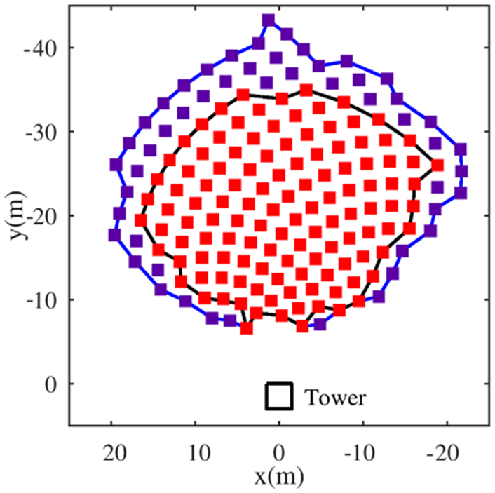
Figure 3.
Tube receptor separation, second optics, vertex sweeps, and angular indicator.
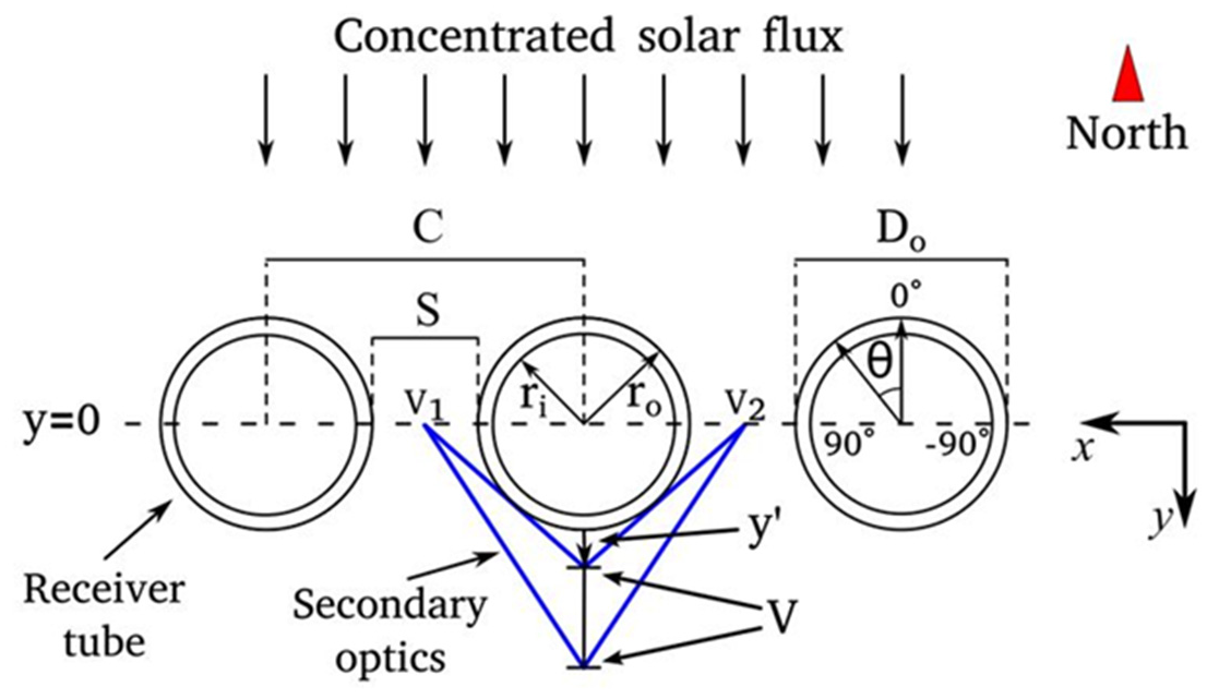
Figure 4.
Ray tracing and CFD results comparison.
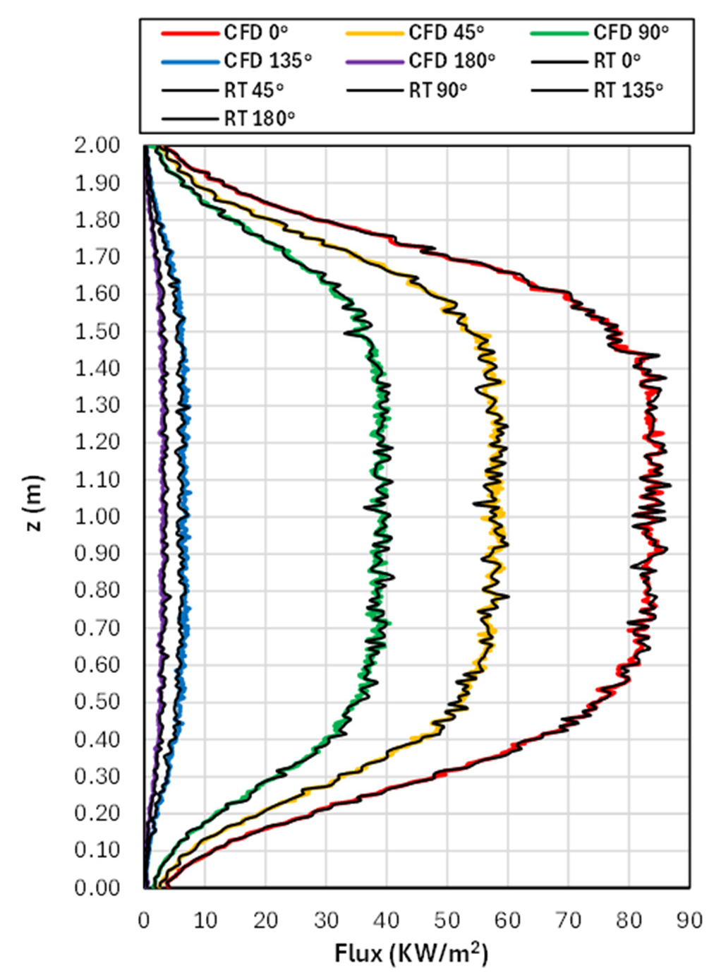
Figure 5.
Flow diagram to compute the average power of each heliostat for selected dates.
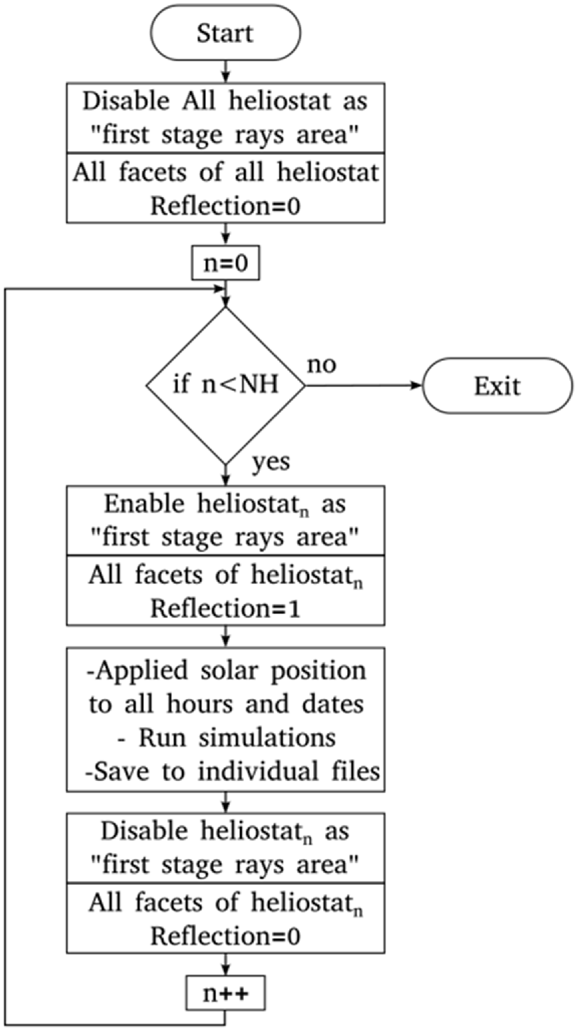
Figure 6.
Computational mesh topology used in the present study.
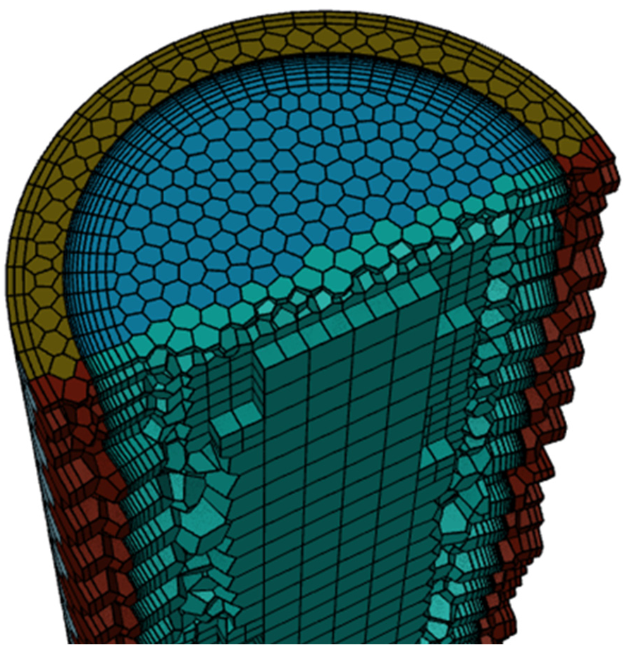
Figure 7.
Temperature profile at z = 0.7 m and θ = 0° using different meshes.
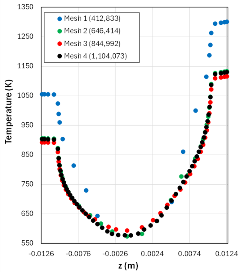
Figure 8.
Validation of the Gnielinski correlation by comparison with simulation results for different Reynolds numbers.
Figure 8.
Validation of the Gnielinski correlation by comparison with simulation results for different Reynolds numbers.
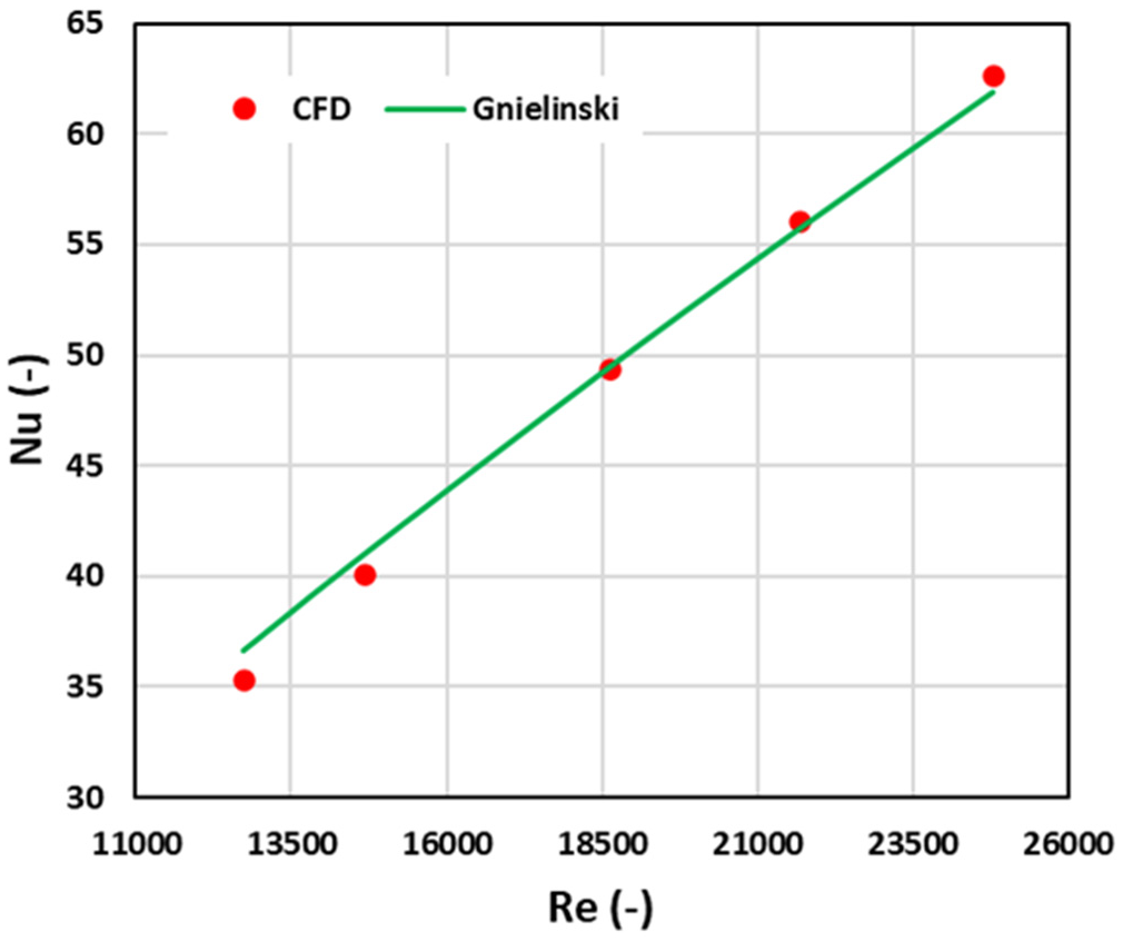
Figure 9.
Flux contours for different hours and days of the year. Winter solstice (left), Spring equinox (center), and summer solstice (right).
Figure 9.
Flux contours for different hours and days of the year. Winter solstice (left), Spring equinox (center), and summer solstice (right).
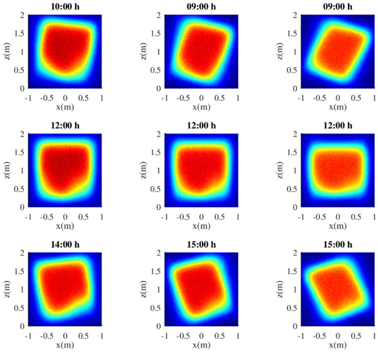
Figure 10.
Flux profile in tube with second optics at z=1 m (separation vertex of 4 mm), for spring equinox at noon.
Figure 10.
Flux profile in tube with second optics at z=1 m (separation vertex of 4 mm), for spring equinox at noon.

Figure 11.
Variation of the optical efficiency of the heliostat field with the vertex distance.
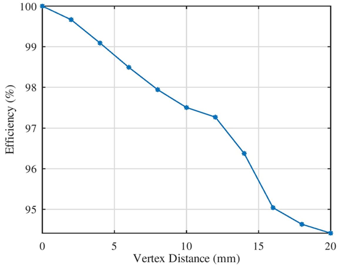
Figure 12.
Flux profile in tube with second optics at z=1 m (separation vertex of 4 mm), for different hours and days of the year.
Figure 12.
Flux profile in tube with second optics at z=1 m (separation vertex of 4 mm), for different hours and days of the year.
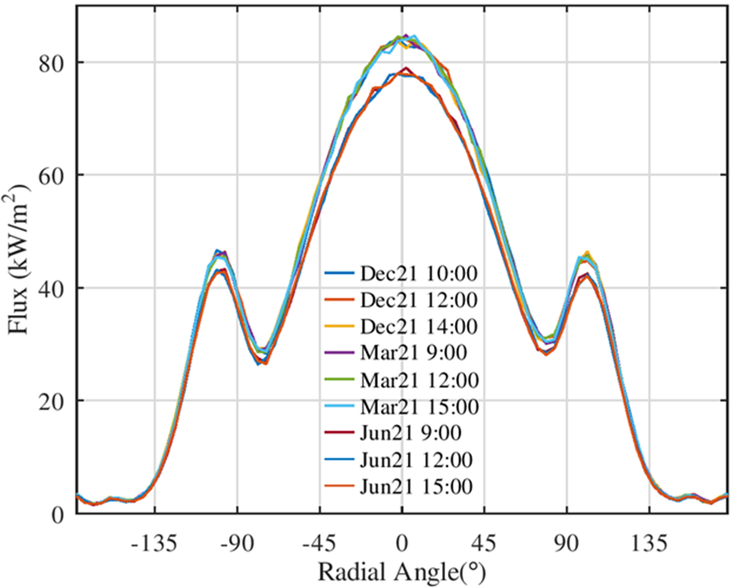
Figure 13.
Vertical temperature profiles on the front face of the solar receiver (θ=0°) for different rear reflector configurations.
Figure 13.
Vertical temperature profiles on the front face of the solar receiver (θ=0°) for different rear reflector configurations.
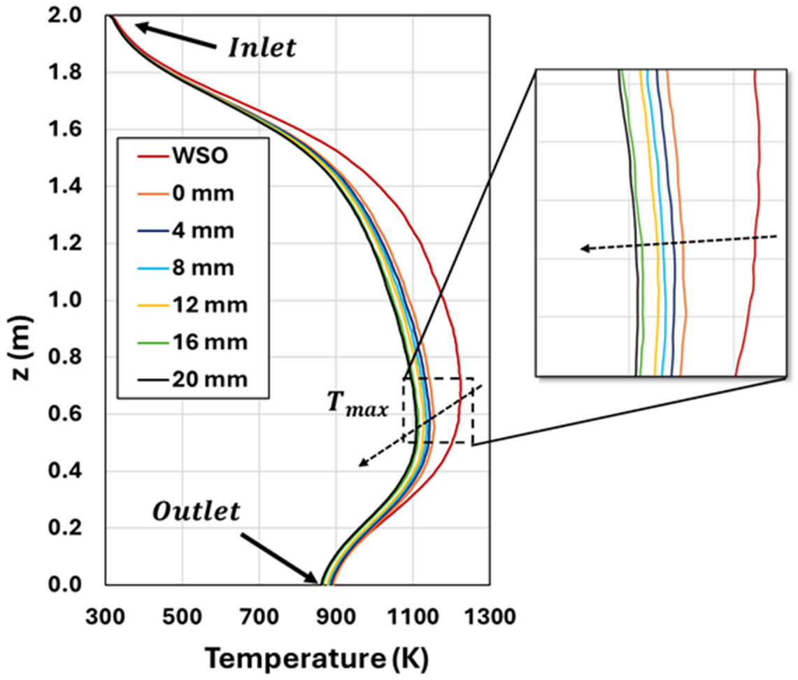
Figure 14.
Axial profile of average fluid temperature in the receiver for the different rear reflector configurations.
Figure 14.
Axial profile of average fluid temperature in the receiver for the different rear reflector configurations.
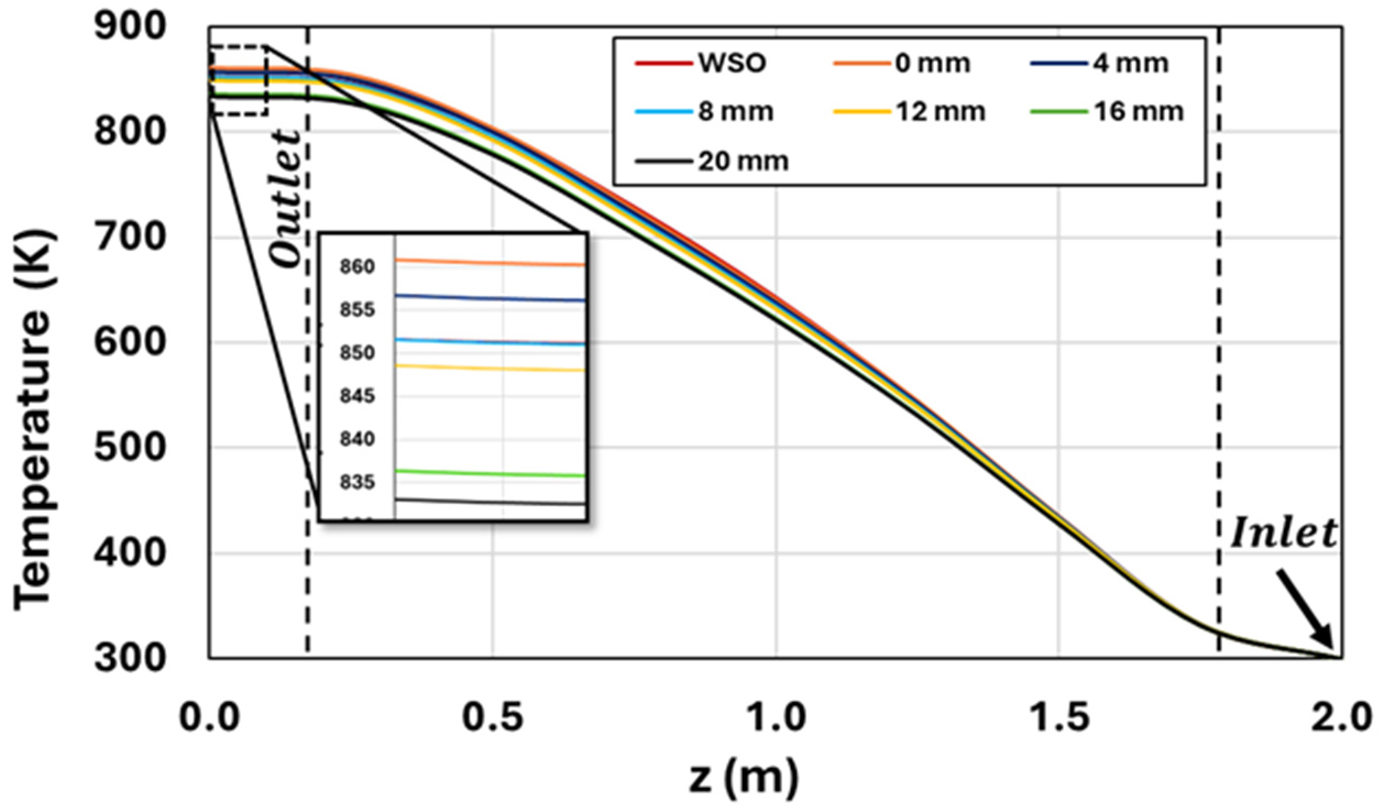
Figure 15.
Axial profile of the average fluid velocity in the receiver for the different configurations studied.
Figure 15.
Axial profile of the average fluid velocity in the receiver for the different configurations studied.
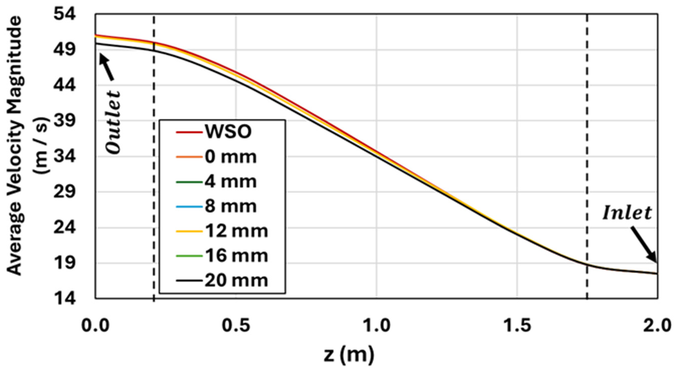
Figure 16.
Radial temperature profile at the solar receiver (z = 1 m, Do =25.4 mm) with different rear reflector configurations.
Figure 16.
Radial temperature profile at the solar receiver (z = 1 m, Do =25.4 mm) with different rear reflector configurations.
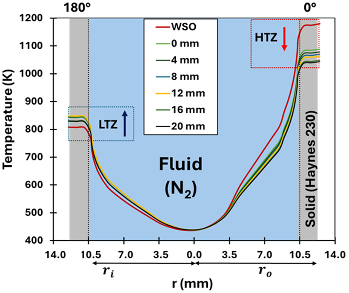
Figure 17.
(a) Radial temperature gradients at the tube cross-section (z = 1 m) and (b) corresponding thermal symmetry ratio (R) for various rear reflector configurations in the solar receiver.
Figure 17.
(a) Radial temperature gradients at the tube cross-section (z = 1 m) and (b) corresponding thermal symmetry ratio (R) for various rear reflector configurations in the solar receiver.
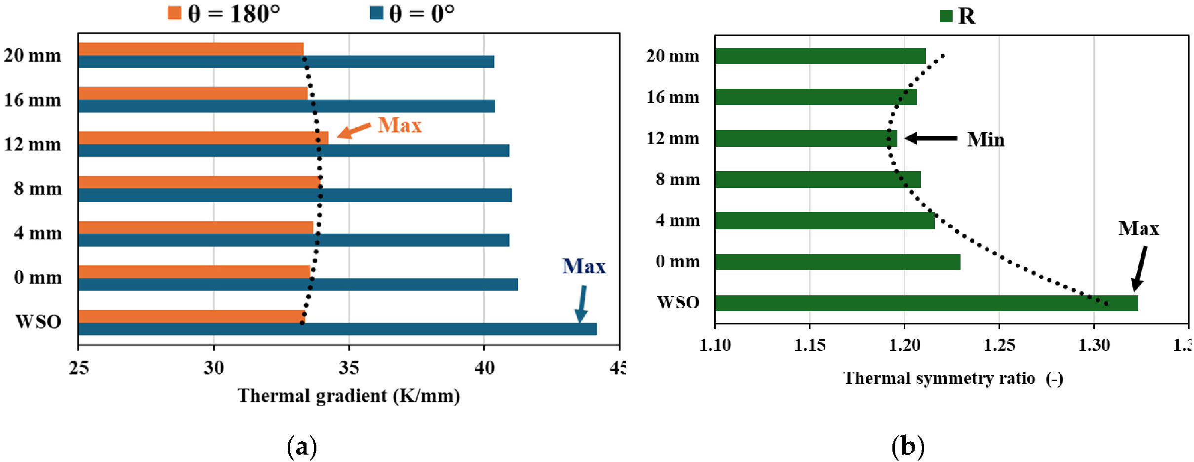
Figure 18.
Vertical profile of the surface temperature ratio (ro, θ=0°/ro, θ=180°) in the receiver tube for different rear reflector configurations.
Figure 18.
Vertical profile of the surface temperature ratio (ro, θ=0°/ro, θ=180°) in the receiver tube for different rear reflector configurations.
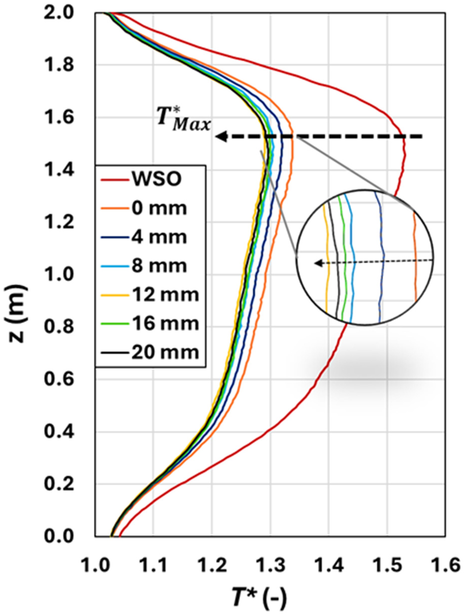

Table 1.
Solar declination with approximate dates..
| Season | Declination (degrees) | Approximate day |
| Winter Solstice (WS) | -23.5 | December, 21 |
| Spring Equinox (SE) | 0 | March, 21 |
| Autumn Solstice (AS) | 23.5 | June, 21 |
| WS-SE | -11.75 | February, 18 |
| SE-AS | 11.75 | April, 20 |
Disclaimer/Publisher’s Note: The statements, opinions and data contained in all publications are solely those of the individual author(s) and contributor(s) and not of MDPI and/or the editor(s). MDPI and/or the editor(s) disclaim responsibility for any injury to people or property resulting from any ideas, methods, instructions or products referred to in the content. |
© 2026 by the authors. Licensee MDPI, Basel, Switzerland. This article is an open access article distributed under the terms and conditions of the Creative Commons Attribution (CC BY) license (http://creativecommons.org/licenses/by/4.0/).
Copyright: This open access article is published under a Creative Commons CC BY 4.0 license, which permit the free download, distribution, and reuse, provided that the author and preprint are cited in any reuse.


