Submitted:
10 February 2026
Posted:
10 February 2026
You are already at the latest version
Abstract
Proton exchange membrane fuel cells (PEMFCs) are promising energy conversion devices owing to high efficiency and zero local emissions. Accurate PEMFC performance assessment and control require well-posed models, whose predictive accuracy is largely determined by the correct calibration of key parameters. Metaheuristic algorithms (MHAs) have therefore been widely applied to PEMFC stack parameter estimation, but their rapid proliferation calls for a more systematic and fine-grained synthesis. This review refines the taxonomy of PEMFC mathematical modeling approaches and summarizes Zero-Dimensional PEMFC modeling methods, key parameters, and representative improvement directions aimed at reducing identification difficulty while retaining physical meaning. Newly developed MHAs and enhanced variants of existing methods are then surveyed, and over 40 distinctive optimization approaches are selected for systematic comparison. Key fuel-cell parameters, evaluation criteria, and representative commercial PEMFC types are summarized. In addition, 26 representative algorithms and their variants are compiled and benchmarked across the five most widely used commercial PEMFC models to enable cross-model comparison.
Keywords:
proton exchange membrane fuel cell
; steady-state polarization modeling
; parameter identification
; optimization algorithms
1. Introduction
In recent years, the urgent need for clean energy sources has grown significantly due to the severe environmental impact of fossil fuels. As a result, renewable energy sources (RES) such as fuel cells (FC), solar, and wind energy are becoming important alternatives due to their advantages of zero emissions, high efficiency, and wide applicability across various scales[1].
Among these types, hydrogen energy, in particular, stands out for its efficiency and sustainability[2]. Among them, proton exchange membrane fuel cells (PEMFC) are notable for their ability to maximize hydrogen energy use, offering low operational pressure, high energy density, and zero emissions[3]. They also have rapid startup, consistent efficiency, long lifespan, and fast charging, making them suitable for diverse applications, from portable systems to transportation[4]. The integration of hydrogen and fuel cells, especially PEMFCs, is critical for achieving sustainable energy solutions, addressing growing energy demands, and reducing environmental impacts[5].
To clarify the position of PEMFCs within the broader fuel cell technology landscape, the main FC types are briefly summarized in Table 1. Fuel cell (FC) systems encompass a range of technologies, including alkaline fuel cells (AFC), molten carbonate fuel cells (MCFC), phosphoric acid fuel cells (PAFC), proton exchange membrane fuel cells (PEMFC), direct methanol fuel cells (DMFC) and solid oxide fuel cells (SOFC), each with distinct characteristics that are systematically compared in Table 1. Among these, PEMFCs have received particular attention due to their high efficiency, low operating temperature, and quick startup behavior. The PEMFC system is inherently a highly nonlinear, multi-variable, and strongly coupled system, with its behavior significantly influenced by changing operating conditions[6,7]. To effectively evaluate and utilize PEMFC systems, researchers have proposed various modeling strategies, including mechanistic (white-box)[6], empirical (gray-box)[7], and data-driven (black-box)[8] approaches. Conventional modeling methods, though widely used, often fall short in addressing this complexity due to their limited adaptability.
Some traditional approaches typically struggle with accurately capturing the system’s dynamic response, leading to increased computational costs and reduced modeling efficiency9,10. As a result, there is a growing demand for more flexible and robust modeling techniques that can effectively handle such challenges. Springer[11] and Bernardi[10] proposed a one-dimensional model in the early 1990s: the former designed a model based on the membrane water content and electrode water vapor balance conditions, while the latter derived a mathematical model of the polymer electrolyte attached to the gas diffusion electrode and pointed out that water transport during fuel cell operation is driven by both pressure and electromotive force. Subsequently, two-dimensional models were developed to consider mass transfer along the length of the fuel cell. Dannenberg[12] et al. established a two-dimensional mass and heat transfer model to analyze different operating conditions and optimize parameters such as humidification and heat transfer. Hosseini[13] et al. used a two-dimensional agglomerate model to study the effect of bubbles and found that increasing relative humidity enhances the migration of water from the cathode to the anode. In addition, 3D models are now widely used. Ferng and Su developed a three-dimensional, full-cell CFD model to examine how flow-field design influences PEMFC performance[14]. Zhang[15] et al. adopted a 3D comprehensive multiphase anisotropic model to study the influence of GDL anisotropy, liquid saturation jump, and baffles inserted to the cathode channel on the performance of PEMFC. Table 2 outlined the dimensional classification of PEMFC models and their characteristics. In the PEMFC model classification system mentioned above, the 0-D model is widely used because of its low computational cost, and ease of rapid fitting with experimental data such as polarization curves. Among various 0-D modeling methods, the semi-empirical model developed by Amphlett is widely adopted due to its effectiveness in capturing the voltage–current (V–I) characteristics of PEMFCs under different operating conditions. This gray-box model combines physical mechanisms with data-driven features and can be used to simulate thermal conduction, mass transport, and electrochemical behaviors within the fuel cell stack[7]. While it does not offer a complete physical interpretation, it provides accurate output prediction with relatively low computational complexity. In addition, the complexity of PEMFC behavior has led to increasing interest in black-box models based on artificial intelligence and neural networks, which are capable of learning system dynamics directly from data without explicit knowledge of internal processes[16,17].
In recent years, the development of computer-based methods and artificial intelligence has facilitated the emergence of metaheuristic algorithms (MHAs) as powerful tools for solving complex optimization problems[16]. Parameter identification in PEMFCs, essentially an optimization task involving multiple unknowns, benefits greatly from the adaptive search mechanisms of MHAs. These algorithms are capable of finding optimal solutions with high precision while maintaining low computational burden.
As a result, various metaheuristic algorithms have been utilized to estimate the unknown parameters in PEMFC models[17]. Commonly adopted methods include genetic algorithm[18], differential evolution[19], particle swarm optimization[20], salp swarm optimization[21], grey wolf optimization[22], and others. Accordingly, a detailed and systematic survey is necessary to comprehensively analyze and synthesize these metaheuristic-based approaches. An earlier study in[23] reviewed and categorized twenty-eight metaheuristic algorithms for PEMFC parameter estimation and further discussed fifteen representative techniques. In addition, a more recent survey was presented in[24], where presented a more recent survey that summarized twenty-seven up-to-date PEMFC models and discussed thirty up-to-date metaheuristic algorithms.
Therefore, this work presents a comprehensive review of unknown-parameter identification for PEMFC models, incorporating 0-D model formulation and refinement and emphasizing metaheuristic-optimization-based parameter identification, aiming to serve as a consolidated reference for future in-depth investigations. The main contributions are summarized as follows:
- i.
- Refined taxonomy of PEMFC mathematical modeling approaches, with an in-depth summary of 0D model formulation, parameterization, and improvement strategies.
- ii.
- Based on the established PEMFC model taxonomy, the applied metaheuristic algorithms are further categorized, and their suitability for different model structures and identification objectives is systematically discussed.
- iii.
- Five summary tables compile optimization results for the five most commonly used commercial PEMFC models, while a comparative analysis of 26 algorithms and their variants (over 40 metaheuristic approaches in total) is provided, including a formula-level comparison of their iterative update mechanisms.
Section 2 presents the 0-D modeling of PEMFC, including the electrochemical processes and the mathematical framework. Section 3 outlines the identification criteria and commercial models used for parameter estimation. Section 4 thoroughly reviews latest meta-heuristic algorithms for PEMFC parameter identification, with a particular emphasis on summarizing the iterative formulas of different optimization algorithms. Section 5 provides a discussion of the reviewed methods. Finally, Section 6 concludes the paper and highlights future research directions.

Table 1.
Fundamental properties of five representative fuel cells.
| FC Type | Anode | Electrolyte | Fuel | Operating Temp. | Efficiency | Power Output | Startup Time | Pros | Cons |
| Proton Exchange (PEM & HT-PEM)[25,26] | Platinum | Polymer Membrane | Hydrogen | 80–100 °C (176–212 °F), 200 °C (224 °F) |
30–40% | 0.12–30 kW | < 1 minute | Quick startup, Small, Lightweight |
Sensitive to humidity, salinity, cold temperatures |
| Alkaline (AFC) [27,28] |
Platinum or Carbon | Potassium Hydroxide (KOH) | Hydrogen, Ammonia |
60–70 °C (140–158 °F) |
60–70% (80% CHP) |
0.5–200 kW | < 1 minute | Quick startup, Temp resistant, Low-cost ammonia fuel |
Liquid catalyst adds weight, relatively bulky |
| Phosphoric Acid (PAFC)[29,30] | Platinum | Phosphoric Acid (H₃PO₄) | Hydrogen, Methanol |
150–200 °C (336–448 °F) |
40–50% (80% CHP) |
100–400 kW | 10–30 minutes | Stable, Mature technology |
Acid vapor, less power-dense |
| Molten Carbonate (MCFC)[31,32] | Steel/Nickel | Molten Carbonate | Natural gas, Methanol, Ethanol, Biogas, Coal gas |
650 °C (1202 °F) |
50% (80% CHP) |
10 kW–2 MW | 10 minutes | Fuel variety, High efficiency |
Slow response, highly corrosive |
| Direct Methanol (DMFC)[33,34] | Platinum-Ruthenium on Carbon | Polymer Membrane | Methanol | 50–120 °C (122–248 °F) |
20–30% | 0.01–100 kW | < 5 minutes | Simple fuel storage, Compact system, No reformer required |
Low efficiency, Methanol crossover, Expensive catalysts |
| Solid Oxide (SOFC)[19,35,36] | Ceramic | Yttria-Stabilized Zirconia (YSZ) | Natural gas, Methanol, Ethanol, Biogas, |
500–1000 °C (932–1832 °F) |
60% | 0.01–2000 kW | 60 minutes | Fuel variety | Long startup time, intense heat |
Table 2.
Comparison of PEMFC Models.
| Dimension | Spatial description | Main phenomena | Typical type | Main outputs | Strengths | Limitations |
| 0-D[10,11] | No spatial resolution | Empirical polarization (V–I) | No spatial direction | Overall cell/stack voltage–current relationship; Lumped outputs |
Extremely fast; easy parameter fitting; Suitable for system-level studies and control-oriented models |
Minimal mechanistic insight; Cannot capture spatial non-uniformity; Limited for design optimization across varying conditions |
| 1-D[12,13] | One spatial direction | Reaction and transport in MEA/porous media; Charge transfer |
Through-plane; Along-channel |
1-D profiles of species, water, potentials, etc.; Trend of current density along the flow channel and location |
Low cost; Retains key physics along a dominant direction; Efficient for parametric sweeps and sensitivity studies |
Misses in-plane effects (rib/channel); Accuracy depends on effective parameters and simplifying assumptions |
| 2-D[14,15] | Two directions (plane) | Rib/channel effects; Reactant depletion; Water buildup |
Cross-channel; Along-channel |
Distributions of water, temperature, and reactants within the PEMFC (2-D fields) | Captures major non-uniformities (rib/channel and along-channel); Balances fidelity and cost for engineering analysis |
Cannot capture inherently 3-D local effects; Relies on effective averaging in the third direction. |
| 3-D[9] | Full 3-D geometry | Full spatial coupling (multi-physics) |
Full 3-D | Full 3-D fields | Highest spatial fidelity; Best for local phenomena, detailed diagnostics, and geometry/design evaluation |
Highest computational cost; Demanding meshing and parameterization; Often impractical for large parametric studies |
2. PEMFC Zero-Dimensional Model
2.1. Electrochemical Process Mechanism
Figure 1 presents the schematic diagram of a typical fuel cell. At the anode, hydrogen molecules are split into protons and electrons with the assistance of a platinum catalyst. The protons then pass through the proton exchange membrane (PEM) to the cathode, while the electrons flow through an external circuit, generating an electric current and voltage across the load[37,38]. At the cathode, the protons and electrons reunite and react with oxygen, forming water and releasing heat as byproducts of the electrochemical process[39]. The complete reaction occurring within the fuel cell is expressed in equation (1), which can be separated into two half-cell reactions shown in equations (2) and (3), corresponding to the anode and cathode reactions, respectively[40].
2.2. Mathematical Modelling
Figure 2(a) illustrates the different model dimensionalities along with the key components of the cell[41]. Higher-dimensional models provide a more accurate representation of reality but come with increased computational cost. Lower-dimensional models, while sacrificing some spatial detail, often enable the inclusion of more complex physical phenomena. As shown in Figure 2(b), the I–V polarization curve of a single PEMFC consists of three distinct regions: activation losses, ohmic losses, and concentration losses. At low current densities, a steep decline in cell voltage is observed, primarily caused by activation losses resulting from sluggish electrochemical reaction rates. As the current increases, the voltage drop becomes more linear, which is attributed to ohmic losses stemming from the internal resistance faced by protons and electrons. At higher current densities, the voltage declines more sharply again due to reactant depletion, often caused by water accumulation that hinders gas diffusion at the electrodes. This final region is known as the concentration loss region[39].
Fuel cells are multi-physics systems, and PEMFC modeling approaches vary depending on the physical phenomena being addressed[42]. Accurate modeling is crucial for analyzing PEMFC performance under different conditions and reproducing polarization curves. In a zero-dimensional (0-D) framework, spatial variations are neglected and the cell behavior is described using lumped operating variables such as voltage, current, temperature and pressure, together with simple semi-empirical or empirical relations. Although 0-D models cannot resolve spatial non-uniformities, they are computationally efficient and are commonly used to represent polarization behavior and support parameter identification at the system level. Accordingly, the output voltage in Figure 2(b) can be expressed as [7]:
where is the activation overpotential(V), is the ohmic voltage loss(V), is the concentration overpotential(V), and denotes the thermodynamic potential(V),which is given by equations
where is the temperature of cell in Kelvin.
2.2.1. Seven Parameters Model
Among various 0-D strategies, the semi-empirical model proposed by Amphlett and Mann[7] is widely used for its balance between physical insight and empirical accuracy. It effectively captures polarization effects—including thermodynamic potential, activation, ohmic, and concentration losses—despite the system’s complexity, multivariable nature, and strong internal coupling. To implement this formulation, each term must be expressed as an explicit function of operating conditions. and are the partial pressures of hydrogen and oxygen, they can be calculated as (6) and (7) follows [7]:
where and are the relative humidities of the anode and cathode, respectively; and denote the inlet pressures at the anode and cathode in atmospheres (atm); represents the electrode area in square centimeters (cm²); is the cell current in amperes (A); and is the saturation pressure of water vapor in atmospheres, which is given by equation (8) [43]:
The activation voltage drop can be expressed as follows:
where, , , and are the parametric coefficients of the cell model, and denotes the oxygen concentration at the catalytic interface(mol/cm³). The oxygen concentration can be calculated as follows[7]:
The ohmic voltage drop arises from the internal resistance of the fuel cell and can be expressed as follows:
where denotes the equivalent resistance associated with electron conduction through contact interfaces, and represents the equivalent resistance of the membrane related to proton conduction, which can be expressed as (12)and(13)[7]:
where is the specific resistivity of the membrane(Ω⋅cm); denotes the membrane thickness in centimeters (cm) and is an adjustable parameter7,44. The concentration overpotential arises due to variations in reactant concentrations at the electrode surface and can be defined as follows[7]:
where is a parametric coefficient(V), is the actual current density of the cell(A/cm²), and represents the maximum allowable current density. When the current density exceeds , the fuel cell output voltage experiences a sharp drop[39].
It is worth noting that the concentration polarization term may become overly sensitive when applied to high-power PEMFC stack datasets with coarse current steps. In such cases, tends to be overestimated, leading to anomalous behavior in the predicted voltage output. To address this issue, an improved formulation was proposed in [45] to reduce the current sensitivity of , making it more consistent with the gradual variation of reactant concentrations under practical steady-state conditions. Accordingly, the original expression in equation (14) was updated to the improved form in equation (16), which significantly enhances the stability and accuracy of the model output:
The fuel cell stack is constructed by connecting individual cells in series; thus, the total stack voltage can be expressed as
As can be inferred from the aforementioned formulas, at least seven parameters (, , , , , and ) must be assigned to fully define an electrochemical-based model.
2.2.2. Two Parameters Model
Building on the classical seven-parameter framework, the proposed two-parameter 0-D PEMFC model explicitly couples reactant partial pressures with operating pressure and gas utilization[46]. Instead of treating hydrogen and oxygen pressures as fixed inputs, the model calculates effective partial pressures of hydrogen and oxygen in the cell based on inlet conditions (pressure, humidity) and the fraction of reactant consumed in equation (16):
This approach enhances physical realism by accounting for the progressive reduction in fuel and oxidant availability along the flow channels at higher utilization. The gas utilization rate and can be defined as:
where and denote the volumetric flow rates of hydrogen and air, respectively. The constant 60,000 converts the flow rate from standard liters per minute to the international system of units. and are Faraday constant and gas constant. Based on this, the description of activation overpotential can be simplified[46]:
where is reference exchange current density, and denotes charge transfer coefficient with the value range of 0 ~ 1. Compared to the seven-parameter model, this activation overpotential expression better reflects the mechanism of activation loss and requires fewer parameters to be optimized.
3. Identification Criteria and Commercial Models
3.1. Identification Criteria
To fully define an electrochemical model, at least seven parameters must be assigned. The parameters of a fuel cell model change significantly under different operating conditions, and these parameters are strongly interdependent. Additionally, these parameters are typically not listed in the manufacturer's specification sheets and need to be determined through experiments or other methods. As a result, the polarization curve and the nonlinear nature of the model can vary greatly, which increases the difficulty of model identification[47]. Therefore, to efficiently and accurately determine the unknown parameters with minimal effort, this process is treated as an optimization problem and solved using various optimization techniques[43,48] . In summary, the procedures for modeling the PEMFC stacks, based on the information extracted from the datasheet and experimental data, are illustrated in Figure 3.
In parameter identification for PEMFC models, selecting an appropriate fitness function is crucial for accurately determining the unknown parameters[46] .These functions help minimize the error between the model’s predictions and experimental data. Choosing the appropriate fitness function (FF) simplifies the parameter identification process and allows for a clear distinction between different modeling methods, both quantitatively and qualitatively, based on the acceptable range of results. A summary of the most commonly used fitness functions (FFs) for parameter estimation in PEMFCs is presented in Table 3.
It is clear that the features and variables used in different fitness functions vary. For example, some functions use squared formulas to more accurately compute the outcomes, while others apply absolute values to avoid negative results.
3.2. Commercial Models
To accurately evaluate and optimize the performance of PEMFCs, it is crucial to understand both their fundamental features and the parameter limits that govern their behavior[49]. Table 4 presents the fundamental features of different PEMFC types, providing an overview of key characteristics such as membrane area, current density, and operating temperature for various commercial models. This information helps in comparing the specifications and understanding the potential applications of each type of PEMFC. Additionally, the typical lower and upper limits of the PEMFC unknown parameters, commonly used in recent research, are summarized in Table 5[41,50].
4. Meta-Heuristic Algorithms for PEMFC Parameter Identification
Among various AI-based optimization techniques, metaheuristic algorithms (MHAs) have demonstrated superior accuracy and computational efficiency compared to traditional optimization methods[24,53,58]. Besides, “No Free Lunch Theorem” states that no single metaheuristic algorithm can independently and efficiently solve all engineering problems [60].
So far, numerous metaheuristic algorithms, along with some modifications or variants, have been employed in PEMFC parameter identification. This section highlights the latest research that introduces new metaheuristic algorithms (MHAs) for identifying the unknown parameters of PEMFCs, based on the semi-empirical model presented in [11].
4.1. Evolution-Based Metaheuristic Algorithms
4.1.1. Differential Evolution (DE)
Differential Evolution (DE) is a simple yet powerful population-based evolutionary algorithm[61,62]. After initialization, DE iteratively refines solutions through three stages: mutation, crossover, and selection, which correspond to generating a new vector by differential variation, recombining it with the current solution, and choosing the better one based on fitness, respectively.
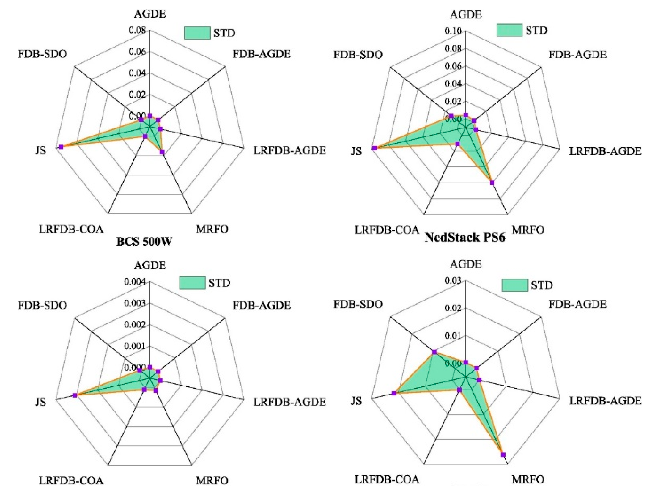
Despite its effectiveness, DE suffers from issues such as slow convergence and parameter sensitivity. To address these issues, various enhanced variants have been developed. One example is Adaptive DE (ADE), which significantly improves search efficiency and helps avoid local optima by introducing two adaptive strategies that enable dynamic adjustment of control parameters[19]. Later, the Adaptive Guided Differential Evolution (AGDE) was proposed as a further enhancement over ADE[63]. It introduced a guiding mutation strategy that utilizes the global best individual to steer the population toward promising regions in the solution space. Furthermore, one recent advancement is the Improved Adaptive Guided Differential Evolution (IAGDE)[64], which not only inherits the adaptive parameter control but also introduces a guided mutation strategy based on the global best solution. This dual improvement enables IAGDE to enhance convergence accuracy while avoiding premature stagnation, making it particularly effective for PEMFC parameter estimation tasks. To evaluate the robustness and stability of different AGDE-based variants across multiple PEMFC models, Figure 1 presents radar plots of the standard deviation (STD) in parameter estimation results, providing a visual comparison of their stability performance[63]. Due to IAGDE's simplicity and robustness, it has been employed in the parameter estimation of the PEMFC model, while the results are gathered in Table 6, Table 7, Table 8 and Table 9.
Figure 1.
Std values for various AGDE-based algorithms of the PEMFCs.
4.1.2. Fish Migration Optimization (FMO)
The design of the Fish Migration Optimization Algorithm (FMOA) is inspired by the migratory life cycle of grayling fish, where individuals gradually evolve from local food searching in early life to long-distance migration in adulthood. In FMOA, the population is divided into five age stages (from 0+ to 4+), and the survival and reproduction of individuals are determined by their fitness and migration energy[77]. Through simulated natural selection and aging mechanisms, fish evolve across generations to explore the search space. However, the original FMOA suffers from weak exploitation and insufficient convergence accuracy. To address these limitations, To address these limitations, researchers proposed an Improved Fish Migration Optimizer (IFMO)[78]. Two key strategies were introduced: a linearly decreasing weight factor to balance global exploration and local exploitation dynamically, and a modified position update formula that guides the search using both the current best individual and the differential information between randomly selected peers. The improved update rule is given by equation
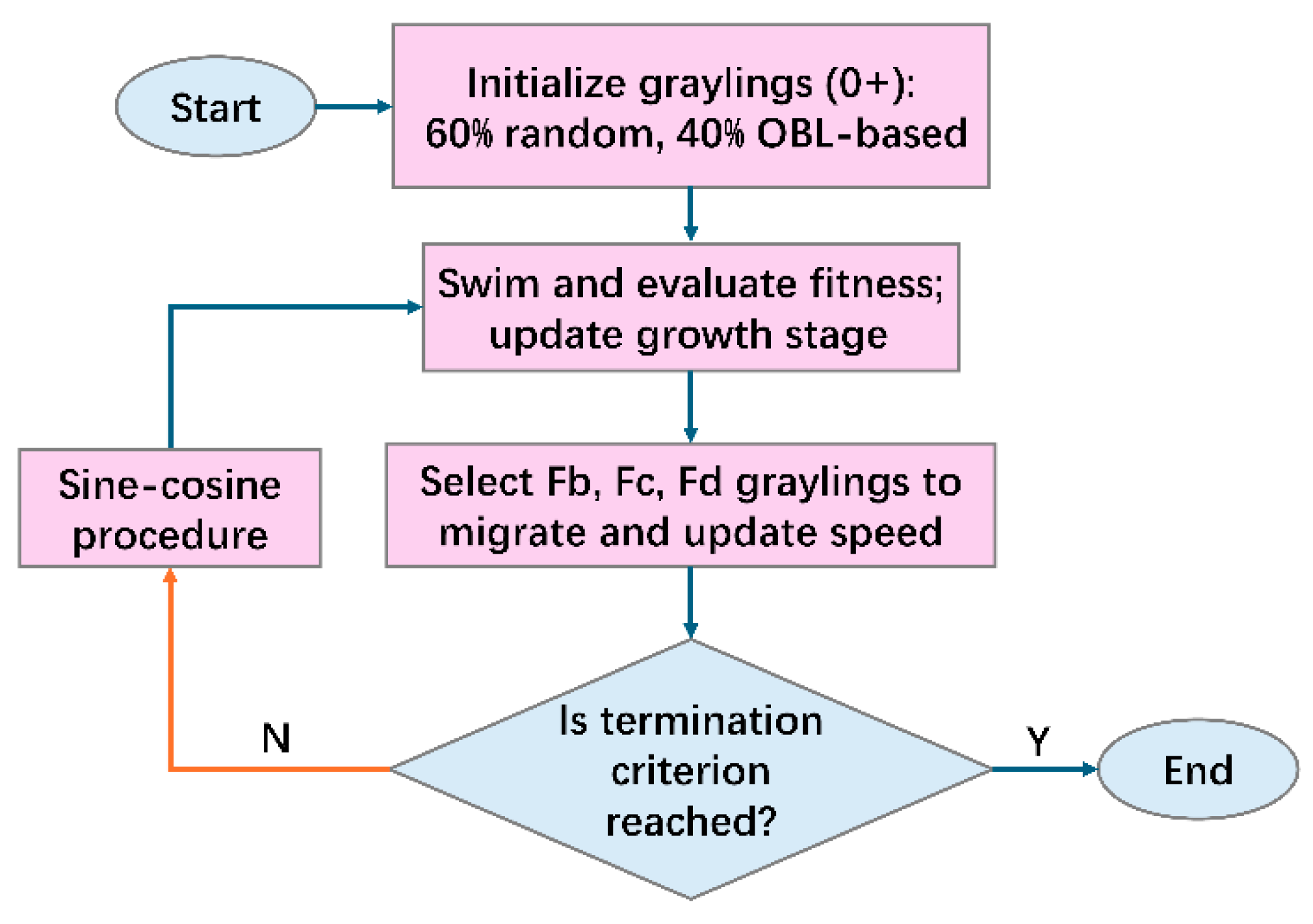
Third, the algorithm uses Opposition-Based Learning (OBL) during initialization—40% of the individuals are generated by reflecting positions across the search space center—to enhance diversity. In addition, a Sine-Cosine mechanism is applied in the migration phase to enrich search trajectories. These enhancements significantly improve the convergence speed, precision, and robustness of IFMO in PEMFC parameter estimation. The overall process of the Improved Fish Migration Optimizer (IFMO) is illustrated in . Due to IFMO’s enhanced convergence precision and balanced search dynamics, it has been employed in the parameter estimation of the PEMFC model, while the results are gathered in Table 9.
Figure 5.
The general flowchart of IFMO.
4.2. Swarm Intelligence Metaheuristic Algorithms
4.2.1. Black Kite Algorithm (BKA)
The Black Kite Algorithm (BKA) is inspired by the hunting and migratory behavior of black kites. It operates in two main phases: the predation phase, where the kites adjust their positions using a sinusoidal strategy to explore the search space, and the migration phase, where they converge toward the best solution found so far[79]. The update mechanism is given by equation
In this context, represents the position of the -th black-winged kite in the -th dimension after the t+1-th iteration following its predation of prey, while denotes the position of the same kite in the jth dimension after the -th iteration. Although BKA performs well, it suffers from premature convergence and lack of diversity early on. To address this, the Improved Black Kite Algorithm (IBKA) was introduced, building upon BKA’s structure. IBKA integrates chaotic opposition-based learning (COBL) for better initial population diversity, Lévy flight for more effective exploration, and a nonlinear decreasing inertia weight to balance exploration and exploitation [59]. These improvements lead to faster convergence and greater accuracy in parameter identification. Due to IBKA’s strong global exploration and convergence capabilities, it has been employed in the parameter estimation of the PEMFC model, while the results are gathered in Table 9.
4.2.2. Red-Billed Blue Magpie Optimizer (RBMO)
The Red-Billed Blue Magpie Optimizer (RBMO) is inspired by the cooperative foraging behavior of red-billed blue magpies. These birds hunt in groups, using a combination of exploration and exploitation to locate, pursue, and store food. In the algorithm, the exploration phase involves searching for new solutions, while the exploitation phase focuses on refining the best solutions found[68]. The update rule for RBMO is given by equation
where is the position of the -th agent, is a random factor, and is the position of a randomly selected agent[68]. This algorithm excels in balancing the global search for new solutions with the local refinement of the best-found solutions. Due to RBMO’s efficient balance between exploration and exploitation, it has been employed in the parameter estimation of the PEMFC model, while the results are gathered in Table 6.
4.2.3. Manta Ray Foraging Optimization (MRFO)
The Manta Ray Foraging Optimization (MRFO) algorithm is inspired by the foraging strategies of manta rays, which include chain foraging, cyclone foraging, and somersault foraging. In chain foraging, individuals follow leaders to form a guided search path; cyclone foraging simulates spiral movements around food sources, promoting exploration; and somersault foraging allows individuals to jump toward or away from the best positions found so far. These strategies are translated into three mathematical operators that govern MRFO’s position updates during optimization[80].
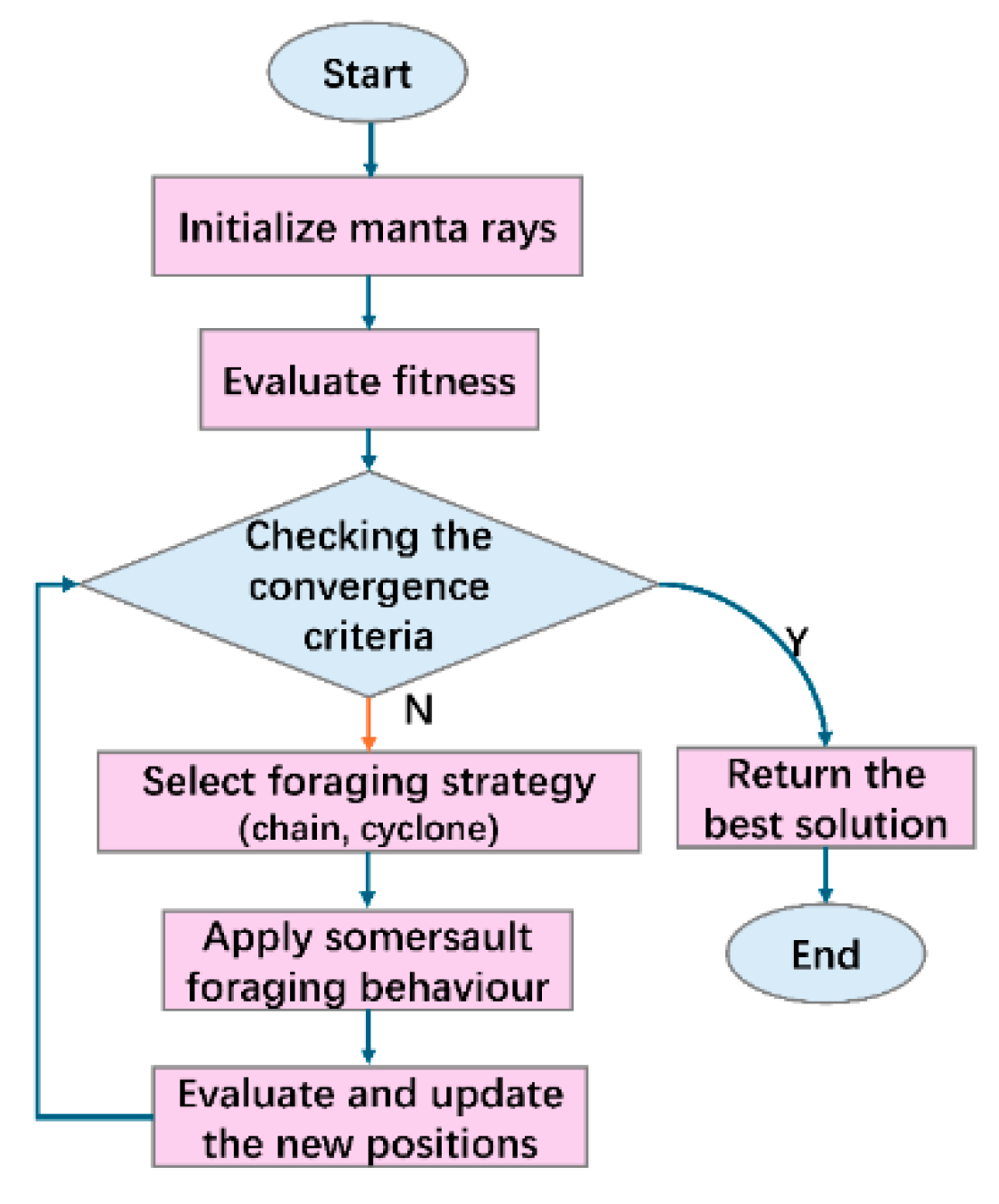
While MRFO balances exploration and exploitation effectively, it suffers from low population diversity and a tendency toward premature convergence, especially in high-dimensional, nonlinear problems like PEMFC parameter identification. To improve its performance, the Modified MRFO (MMRFO) incorporates a sine–cosine mechanism into the chain and cyclone foraging stages [80]. This enhancement modifies the original update formulas to increase the algorithm’s global exploration during the early phase and local exploitation during the later phase. By generating candidate solutions that fluctuate both toward and away from the current best solution, the sine–cosine component helps avoid premature convergence[80]. An overview of the MMRFO workflow is provided in Figure 2. Furthermore, MMRFO enables adaptive switching between chain and cyclone foraging based on the improved equations, providing better search dynamics across the optimization process. Due to MMRFO’s adaptive switching and enhanced search dynamics, it has been employed in the parameter estimation of the PEMFC model, while the results are gathered in Table 7-9.
Figure 2.
Flowchart of the MMRFO.
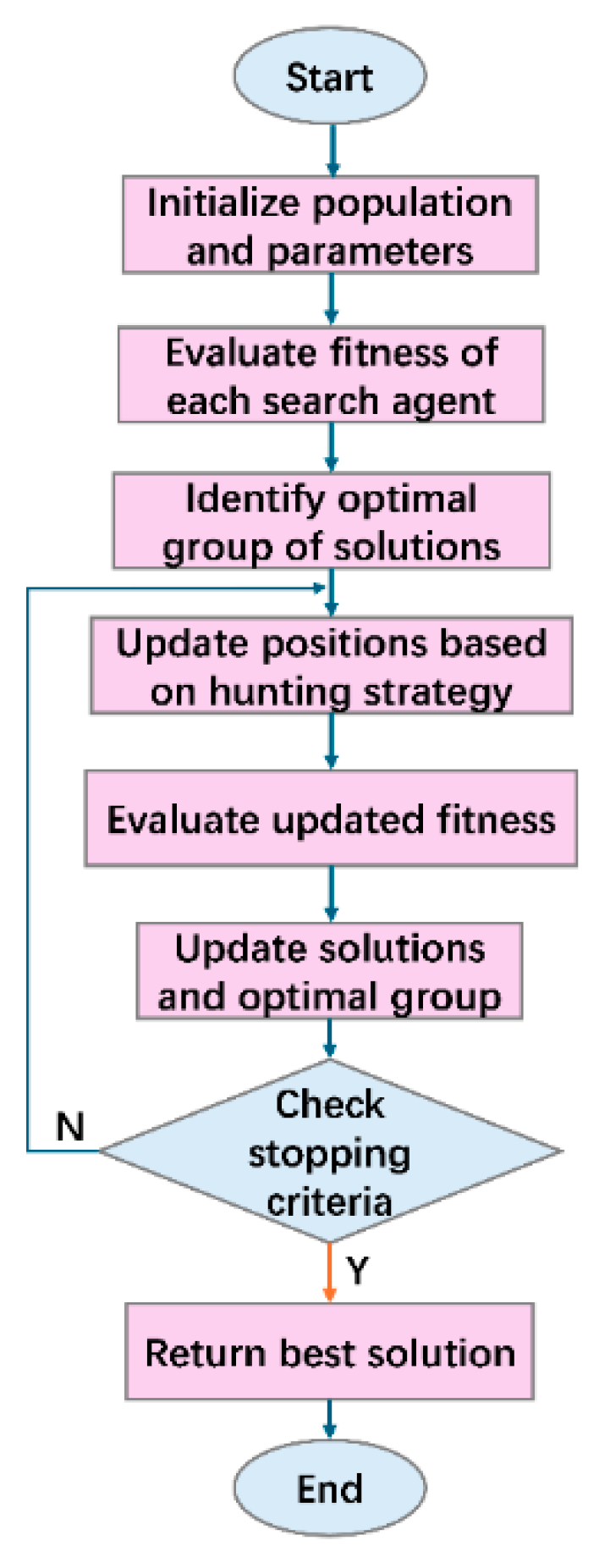
4.2.4. Spotted Hyena Optimizer (SHO)
The Spotted Hyena Optimizer (SHO) is inspired by the hunting behavior of spotted hyenas, which involves group coordination, circling, and attacking prey[70]. In this algorithm, each solution is treated as a hyena, and the optimization mimics the group’s ability to cooperatively encircle and converge toward prey. The core update mechanism is defined by equation
where is the position of a hyena (solution), is the position of the prey (best solution found so far), and , are coefficient vectors that regulate the balance between exploration and exploitation[70]. Additionally, Figure 3 depicts the overall procedure of the SHO algorithm. This formulation enables SHO to adjust its search dynamically depending on how close or far the agents are from the global optimum. Due to SHO’s cooperative hunting-inspired convergence mechanism, it has been employed in the parameter estimation of the PEMFC model, while the results are gathered in Table 6,8,9.
Figure 3.
Flowchart of the proposed SHO.
4.2.5. Artificial Bee Colony (ABC)
The Artificial Bee Colony (ABC) algorithm simulates the foraging behavior of honey bees through three types of agents: employed bees, onlooker bees, and scout bees[81]. Each agent searches the solution space and evaluates nectar quality (fitness), updating positions based on the difference with a randomly selected peer. The original position update rule is equation
where ∈ [−1,1] is a random coefficient and is the position of a randomly chosen solution. Despite its simplicity and global search capacity, ABC suffers from slow convergence and weak local exploitation near the optimum[81].
To overcome these limitations, an Improved Artificial Bee Colony (IABC) algorithm introduces crossover and mutation strategies inspired by GA and DE[83]. In the employed bee phase, a dual-strategy update is applied based on the fitness probability , as defined in equation
In the onlooker bee phase, a DE-like mutation mechanism is used, just as equation follows:
These enhancements greatly improve convergence speed, solution quality, and robustness. When applied to PEMFC parameter identification, IABC achieves lower error and faster convergence than traditional ABC, PSO, and Bayesian optimization. Due to IABC’s dual-strategy update and fast convergence, it has been employed in the parameter estimation of the PEMFC model, while the results are gathered in Table 9.
Table 7.
PEMFC parameter estimation using SR-12 500W PEMFC dataset.
| Years | Methods | Parameters | SSE | ||||||
|---|---|---|---|---|---|---|---|---|---|
| ×10-3 | ×10-5 | ×10-4 | ×10-4 | ||||||
| 2025 | IAGDE[64] | -1.1489 | 3.9900 | 9.2500 | -0.0010 | 13.0000 | 0.0149 | 0.1633 | 6.1350 |
| 2025 | PO[65] | -1.1052 | 3.0679 | 3.6176 | -0.9540 | 24.0000 | 4.7655 | 0.1794 | 1.0072 |
| 2025 | PO[66] | -0.8959 | 2.4210 | 3.6000 | -0.9500 | 23.0000 | 6.7300 | 0.1753 | 0.2424 |
| 2024 | OL-GOOSE[84] | -0.2294 | 1.0770 | 8.2300 | -0.9540 | 23.5065 | 8.0000 | 0.1739 | 1.3310 |
| 2024 | HMO[85] | -0.9364 | 2.9547 | 6.5378 | -1.0632 | 22.6025 | 2.8713 | 0.1501 | 0.0001 |
| 2024 | MMRFO[86] | -1.1914 | 3.8170 | 6.3251 | -0.9541 | 21.1078 | 6.7613 | 0.1752 | 1.0566 |
| 2023 | QOBO[87] | -1.0178 | 3.5590 | 9.7710 | -0.9540 | 22.9990 | 6.7230 | 0.1753 | 1.0460 |
| 2023 | CBO[88] | -0.8863 | 2.7936 | 8.9200 | -0.9540 | 10.0000 | 6.7766 | 0.1631 | 1.1171 |
| 2023 | CBO[89] | -1.1619 | 3.5759 | 5.3503 | -0.9540 | 23.0000 | 1.0000 | 0.1523 | - |
| 2023 | IAHA[71] | -0.8554 | 2.4000 | 3.6000 | -1.0600 | 21.5388 | 2.7300 | 0.1500 | 0.00015 |
| 2022 | BES[90] | -0.8845 | 2.5870 | 5.1800 | -1.0200 | 24.0000 | 5.8200 | 0.1471 | 0.03510 |
| 2021 | MAEFA[91] | -1.1155 | 3.3490 | 4.4000 | -0.9500 | 15.5857 | 8.0000 | 0.0818 | 0.5607 |
| 2021 | HHO[92] | -0.8543 | 2.4162 | 4.2195 | -0.9554 | 13.2011 | 3.5029 | 0.1766 | 1.0678 |
| 2020 | ISSA[93] | -1.1589 | 4.1455 | 5.6443 | -2.2908 | 13.7793 | 1.0000 | 0.0742 | 0.7916 |
| 2020 | VSDE[94] | -0.8576 | 3.0100 | 7.7800 | -0.9540 | 23.0000 | 1.3390 | 0.1516 | 1.2660 |
| 2019 | SSO[21] | -0.9664 | 2.2833 | 3.4000 | -0.9540 | 15.7969 | 6.6853 | 0.1804 | 1.5170 |
| 2019 | FPA[75] | -1.0509 | 3.4000 | 6.5880 | -1.0622 | 12.7962 | 1.9101 | 0.2256 | 0.0019 |
| 2019 | WOA[76] | -0.8902 | 3.3088 | 9.7546 | -1.0330 | 22.8311 | 5.6770 | 0.1464 | 0.0018 |
| 2019 | CS-EO[52] | -1.0353 | 3.354 | 7.2428 | -0.9540 | 10.0000 | 7.1233 | 0.1471 | 7.5753 |
4.2.6. Grey Wolf Optimizer (GWO)
The Grey Wolf Optimizer (GWO) is a swarm intelligence algorithm inspired by the hunting behavior and social hierarchy of grey wolves. The population is classified into alpha (best), beta (second-best), delta (third-best), and omega wolves[95,96]. Position updates are guided by the top three wolves and computed using equation [96]:
While GWO is effective in global optimization, it may suffer from premature convergence and inaccurate exploration, especially in complex search landscapes. Several studies have aimed to enhance the standard Grey Wolf Optimizer (GWO) for more effective parameter identification of PEMFC models. Then a repairable GWO (RGWO) was proposed, introducing an elite archive-based repair mechanism to reinitialize stagnating wolves and a nonlinear adaptive control parameter to balance exploration and exploitation[95]. And the WNT-GWO further improved local search accuracy by incorporating a weighted neighborhood trust model, allowing wolves to update positions based on the fitness-weighted influence of neighbors and dynamically adjust leadership roles[97]. These improvements consistently demonstrated superior performance over the conventional GWO in terms of convergence speed, accuracy, and robustness across different PEMFC parameter estimation tasks. Due to their advantages such as simple tuning process and lower computational time and burden, it has been employed in the parameter estimation of the PEMFC model, while the results are gathered in Table 6,7,10.
4.2.7. Coot Bird Optimizer (CBO)
The Coot Bird Optimizer (CBO) is a metaheuristic algorithm inspired by the social movement patterns of coot birds in flocks[98]. It mimics four behavioral stages: random wandering, adjusted direction toward the group, movement toward the best solution, and collision avoidance[57,99]. The algorithm balances global exploration and local exploitation through these mechanisms[57]. For each subordinate , the position is updated using the following equation :
where denotes the position of the -th coot at iteration ; is the corresponding leader's position; is a uniform random number in (0,1); is a stochastic variable in (1,3), and the cosine term ensures oscillatory convergence behavior. Additionally, elite coots (leaders) are adaptively attracted toward the global best solution , enhancing convergence accuracy and speed[98]. This update rule improves the optimizer’s ability to escape local optima and maintain diversity in complex multimodal search spaces. Due to CBO’s oscillatory convergence and leader-driven dynamics, it has been employed in the parameter estimation of the PEMFC model, while the results are gathered in Table 6, Table 7, Table 8 and Table 9.
4.2.8. Artificial Hummingbird Algorithm (AHA)
The Artificial Hummingbird Algorithm (AHA) is a bio-inspired optimizer that simulates three key foraging strategies of hummingbirds: guided foraging, territorial foraging, and migration[100]. These stages together enable a balance between global exploration and local exploitation. However, the original AHA suffers from slow convergence and a tendency to get trapped in local optima in complex problems such as PEMFC parameter identification. To overcome these issues, the Improved Artificial Hummingbird Algorithm (IAHA) introduces two major enhancements. The first is a Convergence Improvement Strategy (CIS), which enhances the global search and accelerates convergence using the equation nd updatedate rules[71]:
where is the current solution, is the global best, and are uniformly distributed random numbers in [0,1], and is a Levy-distributed vector.
The second enhancement is an Improved Territorial Foraging (ITF) strategy that strengthens exploitation around the best-so-far solution, and its mathematical formulation is expressed in equation
normalized iteration count, , , are random values (uniform or normal), and is a Levy-based scalar[71]. In parallel, the Enhanced Artificial Hummingbird Algorithm (EAHA) was proposed as a variant of AHA. It integrates a dynamically weighted sine–cosine mechanism into the migration phase to further strengthen the global search capability[71]. This design enables the population to escape local optima through periodic and nonlinear perturbations, and improves convergence performance in PEMFC parameter estimation tasks. This mechanism enables the population to escape local optima more effectively by introducing periodic and non-linear perturbations, and its mathematical formulation is expressed in equation
where , , ∈ [0,1] are random control parameters. Both IAHA and EAHA independently enhance the performance of AHA by addressing its limitations from different perspectives, and each has demonstrated superior convergence speed and accuracy in PEMFC parameter estimation tasks. Due to IAHA’s ability to overcome local optima and accelerate convergence, they have been employed in the parameter estimation of the PEMFC model, while the results are gathered in Table 6, Table 7, Table 8, Table 9 and Table 10.
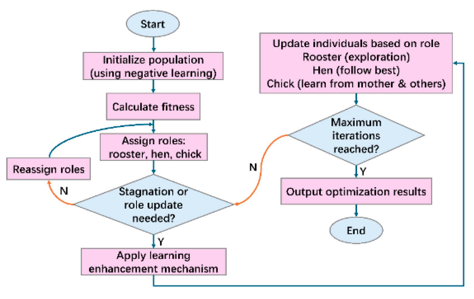
4.2.9. Chicken Swarm Optimization (CSO)
The Chicken Swarm Optimization (CSO) algorithm is a population-based metaheuristic inspired by the social hierarchy and interaction behaviors of chickens. Individuals are categorized into three roles: roosters, hens, and chicks[101,102]. Roosters exhibit independent behavior with stronger exploration, hens follow roosters or better individuals, and chicks follow their mother hens. Although CSO exhibits a good balance between global exploration and local exploitation, it often falls into premature convergence and lacks robustness in complex scenarios like PEMFC parameter estimation. To address these limitations, researchers proposed an Improved Chicken Swarm Optimization (ICSO) algorithm that introduces two enhancement strategies: reverse learning and Levy flight-based disturbance[58]. Due to ICSO’s enhanced diversity and disturbance-based exploitation, it has been employed in the parameter estimation of the PEMFC model, while the results are gathered in Table 6,8Table and Table 9.
Figure 4.
Flowchart of the proposed ICSO.
4.2.10. Bonobo Optimizer (BO)
BO was originally structured around three behavioral phases—positive (PS), negative (NS), and diffusion—mimicking bonobos' decision-making in favorable or hostile environments. However, the original BO lacked adaptivity in parameter tuning and suffered from performance degradation in dynamic search spaces[58]. To overcome these limitations, SABO incorporates a self-adaptive mechanism that dynamically adjusts the control parameter , which governs the influence between social learning and stochastic behavior during the solution update phase. Moreover,The Chaotically based Bonobo Optimizer (CBO) is a refined version of the original Bonobo Optimizer (BO), specifically developed to enhance global exploration capabilities and avoid premature convergence[103]. CBO introduces chaotic dynamics into BO by replacing fixed parameters with values generated from chaos maps such as the logistic or Henon map. The normalized chaotic value is used to dynamically control the individual update behavior. The position update rule is given by equation
where is a chaotic value generated by a map. This adaptive mechanism introduces more diversity into the search process and improves convergence speed and robustness. Due to CBO’s chaotic dynamics and robust convergence, it has been employed in the parameter estimation of the PEMFC model, while the results are gathered in Table 7, Table 8, Table 9 and Table 10.
4.2.11. Whale Optimization Approach (WOA)
The Whale Optimization Algorithm (WOA) is a swarm intelligence algorithm inspired by the bubble-net hunting strategy of humpback whales[104]. It simulates three main behaviors: encircling the prey, spiral updating toward the prey, and searching for prey globally[104,105],. Despite its success in various engineering fields, classical WOA often suffers from slow convergence and insufficient adaptability in high-dimensional problems. To address these limitations, researchers proposed the Enhanced Dimension Learning Whale Optimization Algorithm (EDWOA) by modifying the original WOA position update formula and incorporating two new mechanisms: event-triggered control and dimension learning[104]. In classical WOA, the position update depends on the global best and a fixed update pattern. In EDWOA, this is replaced by a more dynamic form triggered by stagnation events and focused on dimension-wise updates. Its enhanced position update formula is as follows:
where is the position of individual at dimension and iteration ; , are two randomly selected individuals. The dimension learning mechanism ensures that updates are applied selectively to informative dimensions, thus reducing redundancy and accelerating convergence. Due to EDWOA’s dimension-wise control and event-triggered updating, it has been employed in the parameter estimation of the PEMFC model, while the results are gathered in Table .
Table 9.
PEMFC parameter estimation using EDWOA using 250W PEMFC dataset.
| EDWOA | ×10-3 | ×10-5 | ×10-4 | ×10-4 | |||
| Range Set | (-0.952,-0.944) | (0.001, 0.005) | (7.4e-5, 7.8e-5) | (-1.98e-4, -1.88e-4) |
(14,23) | (1.0e-4,8.0e-4) | (0.016,0.05) |
| Extracted Parameters | -0.9440 | 3.0770 | 7.8000 | -1.880 | 23.000 | 1.0000 | 0.0327 |
| SSE | 15.6669 |
4.2.12. GOOSE Optimization Algorithm(GOA)
The GOOSE optimization algorithm is a metaheuristic method inspired by the collective behaviors of geese during foraging and resting periods[106]. In its basic version, the algorithm initializes a population matrix , where each row represents an agent’s position. Out-of-bound solutions are immediately corrected. In each iteration, the algorithm evaluates the fitness of each individual and identifies the best one as and . Despite this balance strategy, the standard GOOSE may still face premature convergence in high-dimensional spaces. To address this, researchers proposed an enhanced variant, called the Orthogonal Learning GOOSE Optimization Algorithm (OL-GOOSE). This variant incorporates an orthogonal learning strategy that systematically generates informative search directions by constructing orthogonal arrays[84]. These arrays allow the algorithm to explore combinations of decision variable values with reduced redundancy and increased efficiency. Instead of purely random updates, the algorithm leverages orthogonally learned solutions to refine its position update process. This enhancement is formulated as equation :
where is the direction learned via orthogonal array experiments, and ∈ [0,1] is a learning rate. By introducing this structure-aware direction into the update mechanism, OL-GOOSE achieves improved convergence speed and robustness in complex optimization tasks such as PEMFC parameter identification. By incorporating structure-aware guidance, OL-GOOSE improves convergence speed and robustness in complex tasks like PEMFC parameter identification. Due to OL-GOOSE’s structure-aware learning and convergence efficiency, it has been employed in the parameter estimation of the PEMFC model, while the results are gathered in Table 7,8,9.
Table 10.
PEMFC parameter estimation using NedStack PS 6KW PEMFC dataset.
| Years | Methods | Parameters | SSE | ||||||
| ×10-3 | ×10-5 | ×10-4 | ×10-4 | ||||||
| 2025 | IAGDE[64] | -1.1846 | 3.6500 | 5.9700 | -0.0007 | 15.7311 | 3.9402 | 0.0136 | 1.2173 |
| 2025 | IBKA[59] | -0.8225 | 2.3000 | 3.9500 | -0.8000 | 13.1539 | 2.1500 | 0.0100 | 0.0715 |
| 2025 | PO[65] | -0.8532 | 2.3988 | 3.6022 | -0.9540 | 13.0947 | 1.0000 | 0.0136 | 2.0862 |
| 2025 | PO[66] | -0.8549 | 2.4380 | 3.8500 | -0.9500 | 14.0000 | 1.2000 | 0.0168 | 0.2752 |
| 2024 | OL-GOOSE[84] | -1.0363 | 2.9300 | 3.6000 | -0.9540 | 13.0223 | 1.0000 | 0.0136 | 2.1042 |
| 2024 | ADSOOA[107] | -1.1710 | 4.4040 | 9.6120 | -0.9540 | 13.3460 | 1.0000 | 0.0136 | - |
| 2024 | HMO[85] | -1.1997 | 3.7318 | 5.9205 | -0.9540 | 13.4650 | 1.0000 | 0.0136 | 2.1457 |
| 2024 | SHO[70] | -0.8532 | 2.4170 | 3.6000 | -0.9540 | 15.7764 | 7.5400 | 0.0323 | 0.1308 |
| 2024 | RIME[108] | -0.8819 | 2.4385 | 3.4000 | -0.9540 | 13.0000 | - | 0.0019 | 1.9459 |
| 2024 | INFO[108] | -1.1976 | 4.0142 | 7.9847 | -0.9540 | 10.0000 | 3.1111 | 0.1611 | 2.2881 |
| 2023 | DO[109] | -1.1082 | 3.4849 | 5.2333 | -0.9530 | 23.0714 | 1.2753 | 0.0836 | 2.0776 |
| 2023 | IABC[83] | -0.9892 | 3.5544 | 8.3970 | -0.9540 | 11.8775 | 1.0000 | 0.0136 | 2.9848 |
| 2023 | CBO[88] | -1.0945 | 2.8818 | 5.6600 | -1.1620 | 16.2870 | 1.0125 | 0.1148 | 1.5734 |
| 2023 | CBO[89] | -1.1706 | 4.4040 | 9.6121 | -0.9540 | 13.3460 | 1.0000 | 0.0136 | - |
| 2023 | IAHA[71] | -0.8831 | 2.6000 | 3.6000 | -0.9500 | 13.4650 | 1.0000 | 0.0136 | 2.1457 |
| 2023 | ICSO[72] | -0.8500 | - | 9.7800 | -0.9560 | 13.3300 | 1.0000 | 0.0130 | 2.1390 |
| 2023 | ARO[73] | -1.0085 | 3.0434 | 4.9796 | -0.9540 | 13.4457 | 1.0000 | 0.0136 | 2.1113 |
| 2022 | ICSO[72] | -0.8760 | 2.6500 | 4.1900 | -0.1028 | 13.0000 | 1.0000 | 0.0530 | 1.8600 |
| 2021 | MAEFA[91] | -1.1490 | 3.3490 | 3.6000 | -0.9500 | 13.0975 | 1.0000 | 0.0136 | 2.0794 |
| 2021 | ASSA[74] | -0.7800 | 3.4400 | 8.2400 | -0.9590 | 13.1300 | 0.1100 | 0.0600 | 2.0300 |
| 2020 | VSDE[94] | -1.1212 | 3.3487 | 4.6787 | -0.9540 | 13.0000 | 1.0000 | 0.0494 | 2.0885 |
| 2019 | FPA[75] | -1.1605 | 4.0000 | 8.4565 | -1.0123 | 15.1264 | 1.2863 | 0.0153 | 0.0983 |
| 2019 | SFLA[55] | -1.0231 | 3.4760 | 7.7883 | -9.5400 | 15.0323 | 1.6200 | 0.0136 | 2.1671 |
4.3. Bio-Inspired Metaheuristic Algorithm
4.3.1. Puma Optimization Algorithm (PO)
The Puma Optimization Algorithm (PO) is a novel bio-inspired metaheuristic algorithm that mimics the predatory behavior of pumas in the wild. PUMAs are solitary hunters that exhibit strategic stalking and pouncing behavior to capture prey[110]. This ecological behavior is abstracted into an optimization framework where each solution is modeled as a puma, and the optimization process emulates hunting through two primary mechanisms: tracking and attacking. In the tracking phase, pumas move in the solution space toward prey positions, using information from better solutions to guide their movement. In the attacking phase, once a target is identified, the puma performs a rapid exploitation maneuver to refine its current position[66]. The position update rule during the attacking phase is given by equation :
where is the position of puma iii at iteration , is the target (best solution), and , are random numbers in [0,1] to maintain exploration diversity. This formula allows a balance between convergence and exploration by dynamically adjusting the puma’s approach toward promising regions in the search space. The algorithm was applied to the parameter identification of PEM fuel cells, and the corresponding results are summarized in Table 6, Table 7, Table 8, Table 9 and Table 10.
4.3.2. Dandelion Optimization Algorithm (DOA)
The Dandelion Optimization Algorithm (DOA) is inspired by the natural dispersal behavior of dandelion seeds. It simulates the life cycle of seeds drifting in air currents through three consecutive stages[111] : fluctuation, rotational drift, and directional motion. In the fluctuation phase, seeds spread randomly under the influence of environmental wind, which encourages global exploration by introducing high randomness, individuals move outward from their current position following a logarithmic spiral flight influenced by wind velocity and humidity. The second phase, rotational drift, guides seeds to rotate around promising regions and transitions the algorithm from exploration to exploitation. This behavior is modeled by a cosine-based update strategy defined as equation :
where is a step size coefficient, and is a randomly selected angle. This equation guides individuals to rotate toward the optimal region, intensifying the exploitation phase. Finally, in the landing phase, individuals perform a Lévy flight around the elite solution to locally refine the search space. To dynamically control the step size during updates, a factor is introduced [109], which applied DOA to the parameter estimation of PEMFCs, where its balance between search phases helped achieve lower sum-of-squares error compared to other metaheuristics, the results are gathered in Table and Table 9. Experimental results demonstrated that this enhancement improves convergence speed and parameter estimation accuracy of the PEMFC model.
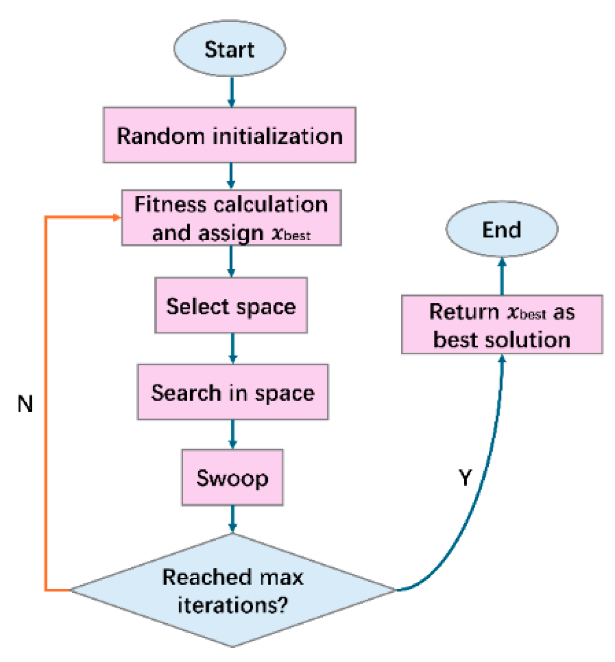
4.3.3. Bald Eagle Search (BES)
The Bald Eagle Search (BES) algorithm is a nature-inspired metaheuristic that mimics the hunting behavior of bald eagles through three sequential phases: selecting space, searching within that space, and swooping. In the first phase, the eagle chooses a promising region based on statistical information about the population. The second phase focuses on exploration around the center of the selected space to ensure diversity. The third phase, swooping, guides the individual toward the best-known solution to intensify exploitation. As presented by [90], during the swooping phase, the position update of an individual is governed by the following equation :
where is the global best solution found so far, is a randomly selected individual from the population, is the current position of the individual, and is a scaling factor. The overall procedure of BES is illustrated in the Figure 5. BES has been employed in the parameter estimation of the PEMFC model, while the results are gathered in Table 7.
Figure 5.
Flowchart of the proposed BES.
4.3.4. Parrot Optimizer (PO)
The Parrot Optimizer (PO) is a recently proposed swarm intelligence algorithm that mimics the intelligent behavior and vocal learning dynamics of parrots[65]. Individuals in PO interact via a social communication model where each parrot can imitate successful calls or behaviors from other members of the population. The algorithm operates in a loop of exploration and exploitation phases, where parrots adjust their position based on personal experience, global knowledge, and a vocal learning mechanism. The main position update formula is given as equation [65]:
where is a randomly selected parrot’s position, ∈ [0,1] is a uniformly distributed random number used to introduce stochastic variability, and ∈ [0,1] is a weighting parameter that controls the influence between social learning and random imitation. This formulation allows PO to dynamically balance exploration and exploitation. PO achieved superior robustness and scalability when applied to PEMFC parameter estimation, outperforming traditional methods in convergence speed and prediction accuracy, the results are gathered in Table 6, Table 7, Table 8 and Table 9.
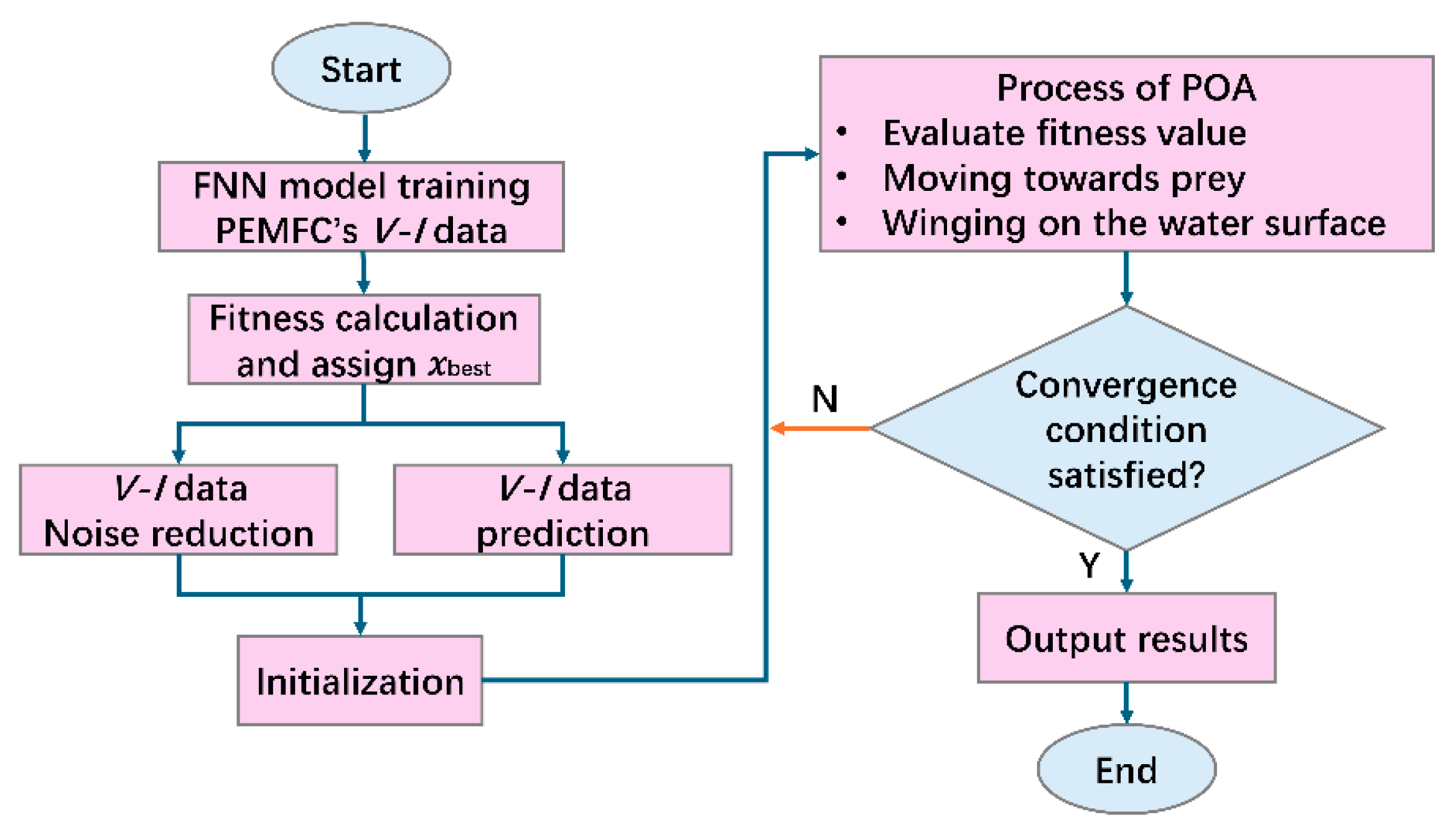
4.3.5. Pelican Optimization Algorithm(POA)
The Pelican Optimization Algorithm (POA) is a nature-inspired metaheuristic algorithm that mimics the cooperative hunting behavior of pelicans. It consists of two main phases: “moving toward the prey,” where individuals explore the search space by approaching promising regions, and “gliding over the water surface,” where fine adjustments are made to exploit the local neighborhood around the best solutions[112]. Moreover, in the literature[67], the feedforward neural network (FNN) is trained to approximate the ideal polarization curve of the PEMFC system using limited and noise-corrupted voltage–current (V–I) data. The key innovation lies in using the FNN as a data preprocessor, which filters out Gaussian and Rayleigh noise from the experimental V–I measurements, providing a denoised target curve. This refined data is then used as the input to POA, which searches for the optimal set of PEMFC parameters by minimizing the RMSE between the FNN-reconstructed curve and the modeled output. Through this two-stage hybrid strategy, the FNN enhances data quality, while POA ensures efficient global parameter optimization. The overall procedure of FNN-POA is illustrated in the Figure 6. Due to FNN-POA’s hybrid strategy with FNN and strong noise immunity, it stands out among various optimization methods for PEMFC parameter identification, with its results presented in Table 6.
Figure 6.
The flow chart of the FNN-POA.
4.4. Physics-based Metaheuristic Algorithms
4.4.1. Archimedes Optimization Algorithm (AOA)
The Archimedes Optimization Algorithm (AOA) is a recently introduced metaheuristic based on the physical principles of buoyant force and fluid dynamics, where candidate solutions are modeled as objects submerged in a fluid medium[113,114]. The algorithm iteratively updates the volume, density, and acceleration of these objects to simulate their motion toward optimal regions in the search space[113,114]. In the study , an improved AOA is applied to estimate the unknown parameters of a PEMFC system. To enhance its convergence and robustness, an improved strategy is embedded during the acceleration update phase, described by the equation [114]:
where is the updated acceleration of the -th object, is its volume, is its density, is the global best solution, is the current position of the object, and is a control parameter. This equation directs individuals toward the best-known solution by leveraging adaptive control over physical properties. As demonstrated in the paper, the improved AOA outperformed other algorithms in terms of precision and convergence when applied to the PEMFC parameter identification task. With its fluid dynamics-inspired convergence behavior, AOA has distinguished itself among multiple approaches in PEMFC modeling tasks, and the relevant performance is reported in Table 8.
4.4.2. Artificial Electric Field Algorithm (AEFA)
The Artificial Electric Field Algorithm (AEFA) is a physics-based metaheuristic that simulates the interaction of charged particles within an electric field, where candidate solutions are treated as charged bodies influencing each other’s motion. AEFA updates the positions and velocities of these particles by computing the resultant electric force and acceleration based on Coulomb's law[115]. To enhance convergence accuracy and speed, researchers proposed a modified version called MAEFA, which integrates an improved velocity update strategy incorporating global and personal best guidance. The modified velocity equation is given as equation [91]:
where is the velocity of the -th particle at iteration , is its acceleration, denotes the global best solution, represents the individual’s personal best, , , are uniformly distributed random numbers in [0,1], and is the inertia weight. This updated strategy enhances the exploitation of the best-found regions while maintaining diversity in the search space. The authors validated the effectiveness of MAEFA through its superior performance in parameter estimation of PEMFC models. Its force-based velocity update mechanism enables it to outperform many conventional algorithms in PEMFC parameter estimation, as evidenced by the results shown in Table 7,8.
Table 8.
PEMFC parameter estimation using BCS 500W PEMFC dataset.
| Years | Methods | Parameters | SSE | ||||||
| ×10-3 | ×10-5 | ×10-4 | ×10-4 | ||||||
| 2025 | IAGDE[64] | -0.6306 | 1.5400 | 3.8100 | -1.9300 | 17.8000 | 16.100 | 0.1991 | 0.0116 |
| 2025 | IBKA[59] | -1.0222 | 3.0000 | 5.8800 | -1.9300 | 20.8637 | 1.0600 | 0.0163 | 0.0119 |
| 2025 | PO[65] | -0.8532 | 2.1800 | 3.6000 | -1.9000 | 20.8772 | 1.0000 | 0.0161 | 0.0255 |
| 2025 | PO[66] | -0.8532 | 2.1793 | 3.6000 | -1.9289 | 20.8145 | 1.0000 | 0.0161 | 0.0126 |
| 2024 | OL-GOOSE[84] | - 1.099 | 3.1900 | 6.0000 | -1.9000 | 23.9986 | 4.0000 | 0.0163 | 0.0117 |
| 2024 | MSMA[116] | -1.1996 | 3.1413 | 3.6003 | -1.9265 | 22.0849 | 2.1398 | 0.0163 | 0.0117 |
| 2024 | HMO[85] | -1.0573 | 3.3155 | 6.9733 | -1.9302 | 20.8769 | 1.0001 | 0.0161 | 0.0117 |
| 2024 | AGPSO[117] | -1.0283 | 3.4000 | 8.2000 | -1.9300 | 20.7300 | 1.1000 | 0.0162 | 0.0107 |
| 2024 | ESSA[118] | -0.8532 | 2.2577 | 3.6000 | -1.9275 | 20.7722 | 1.0007 | 0.0162 | 0.0117 |
| 2024 | MMRFO[86] | -1.1421 | 3.1442 | 4.8535 | -1.9298 | 21.0712 | 1.1625 | 0.0162 | 0.0116 |
| 2024 | AOA[114] | -0.9712 | 2.7704 | 4.3020 | -1.9520 | 19.9760 | 1.7720 | 0.0154 | 0.0123 |
| 2024 | SHO[70] | -1.1995 | 3.2690 | 3.6100 | -2.1000 | 10.1424 | 1.7300 | 0.0309 | 0.0021 |
| 2024 | INFO[119] | -1.1548 | 3.3586 | 5.3564 | -1.9176 | 10.0000 | 1.9130 | 0.0168 | 0.0128 |
| 2024 | SL-PSO[120] | -0.8963 | 4.8000 | 8.6424 | -1.4400 | 17.6400 | 36.300 | 0.1018 | 0.0380 |
| 2023 | IABC[83] | -0.9467 | 3.3973 | 7.5589 | -1.9275 | 20.8709 | 1.1000 | 0.0163 | 0.0117 |
| 2023 | CBO[88] | -1.0922 | 2.8264 | 6.9700 | -1.2120 | 23.1540 | 1.4445 | 0.0141 | 0.0116 |
| 2023 | CBO[89] | -1.1997 | 3.2414 | 3.6000 | -1.9302 | 20.8772 | 1.0000 | 0.0161 | - |
| 2023 | IAHA[71] | -0.8774 | 3.5000 | 9.5600 | -1.9300 | 20.8772 | 1.0001 | 0.0161 | 0.0117 |
| 2023 | ARO[73] | -1.1762 | 3.7344 | 7.3729 | -1.9302 | 20.8772 | 1.0000 | 0.0161 | 0.0117 |
| 2022 | ICSO[72] | -0.8420 | 5.1500 | 9.5400 | -2.7000 | 23.0000 | 3120.0 | 0.0190 | 0.0100 |
| 2021 | HHO[92] | -1.0931 | 3.2804 | 5.6740 | -1.8967 | 20.0436 | 2.2579 | 0.0151 | 0.0149 |
| 2020 | ISSA[93] | -1.0979 | 3.3352 | 5.9034 | -1.9275 | 21.2495 | 1.4823 | 0.0161 | 0.0116 |
| 2020 | VSDE[94] | -1.1970 | 4.2330 | 9.7990 | -0.1920 | 20.1940 | 1.1080 | 0.0157 | 0.0121 |
| 2019 | SSO[21] | -1.0180 | 2.3151 | 5.2400 | -1.2815 | 18.8547 | 7.5036 | 0.0136 | 7.1889 |
| 2019 | CS-EO[52] | -1.1365 | 2.9254 | 3.7688 | -1.3949 | 18.5446 | 8.0000 | 0.0136 | 5.5604 |
| 2019 | FPA[75] | -0.9851 | 2.8000 | 4.4600 | -2.3200 | 17.4598 | 1.6600 | 0.0697 | 0.0164 |
| 2019 | SFLA[55] | -0.9657 | 3.0800 | 7.2236 | -1.9300 | 20.8862 | 1.0000 | 0.0161 | 0.0117 |
4.4.3. Rime-Ice Algorithm (RIME)
The RIME (Rime-Ice) algorithm is a physics-based metaheuristic inspired by the natural phenomenon of rime ice formation in cold environments. It simulates the physical behaviors of nucleation, accumulation, and surface growth of ice particles[108]. In this algorithm, candidate solutions are treated as rime ice particles, and their positions evolve iteratively to simulate the growth and diffusion toward optimal regions. To balance global exploration and local exploitation, RIME introduces an adaptive inertia weight and an exponential fitness-based factor, enabling the algorithm to guide the search adaptively. Researchers applied RIME to the parameter identification of PEM fuel cells, achieving superior convergence precision[108]. The solution update mechanism is expressed as equation follows:
where is a time-decreasing inertia weight, is the fitness of the current solution, is the average fitness of the population. This update mechanism allows high-quality solutions to exert stronger attraction while maintaining population diversity. Thanks to its unique simulation of exponential frost growth and adaptive exploration strategy, RIME has emerged as a competitive algorithm for PEMFC modeling, with outcomes summarized in Table .
4.4.4. Weighted Mean of Vectors Optimizer (INFO)
The Weighted Mean of Vectors Optimizer (INFO) simulates the dynamic generation and combination of weighted vectors to perform global and local search. The algorithm operates in three main phases: updating rules, vector combination, and local search. In the first phase, INFO generates intermediate candidate solutions using a weighted mean of randomly selected vectors combined with a convergence adjustment term (CA)[119], which enhances global exploration. In the second phase, multiple vector-based search strategies are fused to maintain population diversity and improve convergence. The third phase introduces an intensified local search mechanism to fine-tune solutions around promising regions. One of the core update equations applied in PEMFC parameter identification is as equation follows:
where is the position of the -th solution at generation , is the global best solution, is a randomly selected individual, is a scaling factor, and is a normally distributed random value. The term represents the collaborative behavior encoded through the weighted mean of selected vectors. This formulation enhances convergence speed while preserving solution diversity. INFO was successfully applied to identify parameters for three different PEMFC systems and achieved lower standard deviations and sum of squared errors, demonstrating its robustness and accuracy in engineering-level parameter estimation tasks, and its performance in PEMFC parameter estimation is detailed in Table ,9.
4.5. Social-Based Metaheuristic Algorithms
4.5.1. Human Memory Optimizer (HMO)
The Human Memory Optimizer (HMO) is a novel metaheuristic algorithm inspired by human memory processes. It simulates human memory behavior, where individuals remember successful and unsuccessful experiences and adjust their actions accordingly[122]. The algorithm continuously updates its search direction by recalling both successes and failures, with the goal of achieving optimal solutions for optimization problems. The update mechanism of HMO is represented as equation follows[85]:
where denotes the mean position, is a random value between 0.1 and 1.3, and and represent the upper and lower bounds of the search space. The algorithm excels at balancing the exploration and exploitation phases, allowing it to avoid local minima and converge faster. Consequently, the study in employed HMO to estimate the unknown parameters of PEMFCs[85], and the corresponding results are summarized in Table 7,9 and Table 9.
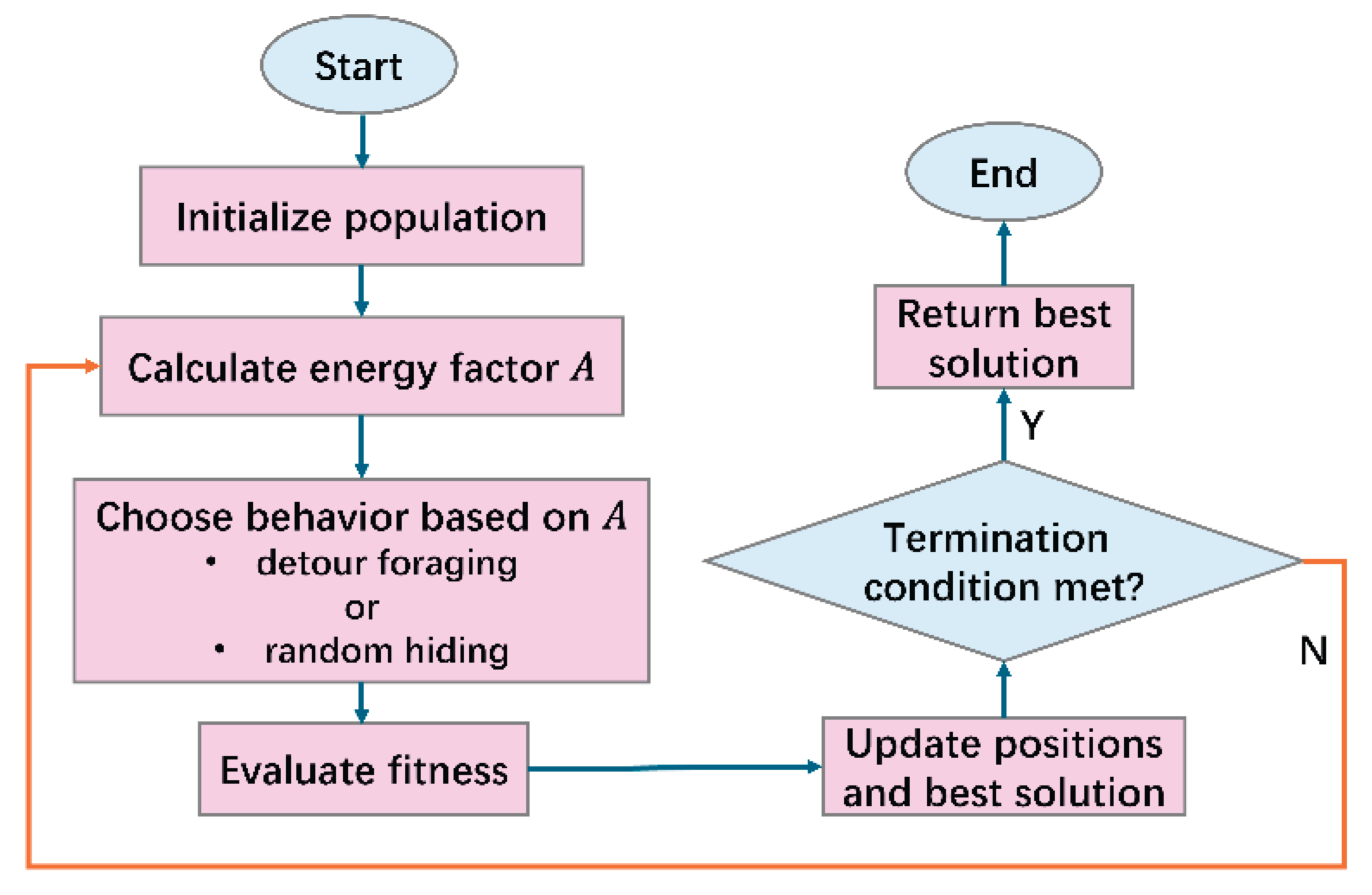
4.5.2. Artificial Rabbits Optimization (ARO)
Artificial Rabbits Optimization (ARO) is a social behavior-inspired metaheuristic algorithm, mimicking the dual behavior of rabbits in nature, namely “hiding” and “running,” which correspond to local exploitation and global exploration[123]. The transition between these behaviors is regulated by a dynamic energy factor ∈ [0,1]. When the energy level is high ( >0.5), the individual performs a local search near its current position, simulating hiding in burrows. When the energy decreases, the individual switches to a running mode, performing broad exploration. Researchers applied ARO to the parameter identification of PEM fuel cells, leveraging its adaptive behavior to improve convergence and accuracy[73]. The core improvement of the ARO algorithm lies in the hiding phase, and its overall procedure is illustrated in . By incorporating dual behavioral modes of hiding and escaping, ARO exhibits superior adaptability compared to many existing algorithms, as reflected in its performance results in Table 6,8,9.
Figure 11.
The flow chart of the ARO.
4.5.3. Social Learning-based Particle Swarm Optimization (SL-PSO)
Social Learning-based Particle Swarm Optimization (SL-PSO) is a socially inspired metaheuristic algorithm that builds upon the classical Particle Swarm Optimization (PSO) by introducing a novel learning mechanism based on social interactions. In the standard PSO, each particle adjusts its trajectory by considering its personal best position and the global best solution found by the entire population. However, this rigid learning framework often limits the diversity of the search process and may lead to premature convergence, especially in high-dimensional or multimodal problems such as PEMFC parameter identification[20].
To address these limitations, SL-PSO incorporates the principles of social learning theory, where particles learn not only from their own experience but also from the observed behaviors of others[120]. Specifically, each particle selects a subset of peers from the population and evaluates their fitness. Among them, the particle with the best performance is chosen as the "social exemplar," denoted as . The velocity and position update rules are then modified to include this exemplar, allowing particles to explore the solution space more intelligently based on socially guided behavior. The modified update rules are as equation and follows:
Here, and represent the position and velocity of particle iii at iteration , is its personal best solution, is the position of the selected social peer, and are random values uniformly distributed in [0,1], and , , are inertia and acceleration coefficients. This socially guided learning strategy enhances both the exploration and exploitation abilities of the swarm by maintaining solution diversity and adapting the search direction based on group-level knowledge. Researchers successfully applied SL-PSO to identify key parameters of proton exchange membrane fuel cells (PEMFCs), and experimental results demonstrated that SL-PSO outperformed conventional PSO in terms of convergence speed, solution accuracy, and robustness[120]. Its results are included in Table 8.
Table 9.
PEMFC parameter estimation using 250W PEMFC dataset.
| Years | Methods | Parameters | SSE | ||||||
| ×10-3 | ×10-5 | ×10-4 | ×10-4 | ||||||
| 2025 | MM-MFO[124] | -0.8000 | 2.3000 | 5.6837 | -1.3587 | 13.9909 | 8.3000 | 0.0100 | 1.0996 |
| 2025 | PO[65] | -0.8603 | 2.2782 | 3.6001 | -1.7382 | 14.4208 | 1.0000 | 0.0138 | 0.3314 |
| 2024 | ESSA[118] | -1.1763 | 3.1115 | 3.6000 | -1.3495 | 11.6174 | 1.0000 | 0.0139 | 0.6013 |
| 2024 | HMO[85] | -1.1041 | 2.9895 | 3.6021 | -1.7389 | 14.4394 | 1.0000 | 0.0138 | 0.3314 |
| 2024 | WNT-GWO[97] | -0.8532 | 2.8105 | 8.0883 | -1.2887 | 14.3197 | 1.6833 | 0.0339 | 7.9547 |
| 2024 | ADSOOA[107] | -0.8490 | 2.4230 | 5.2830 | 1.8800 | 23.0000 | 1.0070 | 0.0292 | - |
| 2024 | MSMA[116] | -1.0986 | 2.7246 | 3.6000 | -1.5603 | 23.0000 | 1.0000 | 0.0545 | 0.6420 |
| 2023 | IFMO[78] | -0.8010 | 2.9620 | 6.0890 | -1.5830 | 14.0000 | 2.6700 | 0.0270 | - |
| 2023 | GTO[125] | -0.9468 | 3.2000 | 7.5200 | -1.7000 | 15.4931 | 1.0000 | 0.0160 | 0.3378 |
| 2023 | DO[109] | -0.9616 | 2.5344 | 3.6000 | -1.3825 | 13.3372 | 4.2320 | 0.0150 | 0.1584 |
| 2023 | CBO[89] | -0.8490 | 2.4220 | 5.2826 | -1.8800 | 23.0000 | 1.0068 | 0.0291 | - |
| 2023 | QOBO[87] | -0.9493 | 2.2890 | 3.6000 | -1.5580 | 23.0000 | 1.0000 | 0.0545 | 0.6355 |
| 2023 | IAHA[71] | -1.0866 | 3.3000 | 5.1000 | -1.7000 | 19.9358 | 1.0000 | 0.0145 | 0.3359 |
| 2023 | ICSO[72] | -1.0700 | - | 7.9100 | -1.5000 | 23.0000 | 1.0000 | 0.0550 | 0.6070 |
| 2022 | BSOA[126] | -0.8560 | 2.6400 | 7.9800 | -1.2100 | 13.2000 | 1.0000 | 0.0333 | 0.7200 |
| 2022 | GBO[127] | -0.9909 | 3.0800 | 7.0000 | -2.1000 | 10.7636 | -4.3900 | 0.0185 | 0.0557 |
| 2021 | CEPSO[128] | -0.8556 | 2.4024 | 5.7420 | -1.5838 | 25.0000 | 1.0000 | 0.0555 | 0.6112 |
| 2021 | IAEO[129] | -0.9991 | 2.8250 | 4.4700 | -1.7000 | 19.9358 | 1.0000 | 0.0145 | 0.3360 |
| 2021 | HHO[92] | -1.1097 | 3.4586 | 8.3168 | -1.5168 | 22.9454 | 3.8308 | 0.0543 | 0.6458 |
| 2020 | ISSA[93] | -0.8616 | 3.1548 | 9.7857 | -1.5423 | 22.8812 | 1.0016 | 0.0547 | 0.6434 |
| 2020 | VSDE[94] | -1.1921 | 3.1990 | 3.7990 | -1.8700 | 22.8170 | 1.2020 | 0.0290 | 1.0526 |
| 2020 | TGA[130] | -1.1914 | 4.1120 | 6.0570 | -1.7090 | 18.6800 | 4.8520 | 0.0544 | 0.7496 |
| 2019 | JAYA-NM[49] | -1.1996 | 3.5500 | 6.0000 | -1.2000 | 13.2287 | 1.0000 | 0.0333 | 5.2513 |
| 2019 | CS-EO[52] | -0.8532 | 2.8121 | 8.1180 | -1.2623 | 14.4722 | 1.0000 | 0.0353 | 8.0665 |
| 2019 | FPA[75] | -0.8775 | 2.5000 | 6.4439 | -1.2531 | 12.0160 | 0.6369 | 0.0198 | 0.2872 |
| 2019 | WOA[76] | -0.9565 | 3.2221 | 8.2328 | -1.7541 | 20.4470 | 1.0820 | 0.0152 | 0.0493 |
| 2019 | SSO[21] | -1.0554 | 3.7953 | 9.8000 | -1.1755 | 24.0000 | 1.0884 | 0.0136 | 1.1508 |
5. Summary and discussion
To facilitate the reader's review of the previously discussed metaheuristic algorithms (MHAs), a comprehensive summary is provided in Table 6, Table 7, Table 8, Table 9 and Table 10. These tables also include several additional algorithms and their variants that have been extensively reviewed in the existing literature; therefore, detailed descriptions of these methods are omitted in this paper.
In recent years, a number of newly metaheuristic algorithms are proposed. Taking the Puma Optimization Algorithm (PO) and the Bald Eagle Search (BES) algorithm mentioned in this paper as examples, they have demonstrated remarkable effectiveness in PEMFC parameter identification. These algorithms offer improved global search capability and faster convergence due to their novel search strategies and hybridized exploration–exploitation mechanisms. For instance, PUMA mimics the cooperative hunting behavior of pumas, dynamically adjusting the movement of candidate solutions based on prey escape patterns, while BES combines migration, attacking, and swooping phases to efficiently cover the solution space. Their ability to adaptively escape local optima and maintain solution diversity throughout the optimization process makes them well-suited to the highly nonlinear and strongly coupled nature of PEMFC models.
In addition to newly developed algorithms, many classical metaheuristics have been enhanced through a variety of well-established improvement techniques tailored to the PEMFC parameter identification problem. These modifications aim to address challenges such as premature convergence, local optima trapping, and limited solution diversity. Commonly employed strategies include chaotic initialization to increase initial solution diversity, opposition-based learning (OBL) to accelerate convergence by evaluating both current and opposite solutions, and Lévy flight mechanisms to enable long-distance jumps in the search space. Other techniques such as adaptive weight adjustment, elitism retention, and Gaussian perturbation improve stability and convergence precision. Furthermore, hybrid strategies, which combine the strengths of multiple algorithms, and mechanisms like escape energy modeling, which is often used in predator-prey-inspired algorithms—further enhance global exploration. These enhancements collectively improve the robustness and search efficiency of classical algorithms, making them better suited for the high-dimensional, nonlinear, and strongly coupled nature of PEMFC models.
The parameter identification task in PEMFC modeling presents several intrinsic challenges, including highly nonlinear behavior, strong coupling between variables, and a complex, multi-modal solution space. These characteristics make it easy for conventional algorithms to fall into local optima or suffer from premature convergence. Moreover, PEMFC performance is highly sensitive to small parameter deviations, which demands robust and precise optimization strategies. Compared to earlier methods, both newly developed algorithms and improved variants offer stronger capabilities in global search, adaptability, and convergence stability. Specifically, effective algorithms for this domain must rapidly cover the search space, maintain solution diversity, and dynamically balance exploration and exploitation to escape local minima and identify globally optimal parameter sets.
6. Conclusions
This paper aims to summarize, classify and compare the metaheuristic methods for PEMFC parameter estimation in detail from the aspects of application year, application method, usage data, advantages and disadvantages and PEMFC cell type. And the following suggestions are made for the direction of in-depth research in related fields in the future:
In summary, the problem of PEMFC parameter identification fundamentally involves four key elements: the PEMFC model, the optimization algorithm, the dataset, and the objective function.
Among these, optimization algorithms have seen rapid advancements in recent years, with a growing number of novel and hybrid metaheuristic techniques being applied. Also, other approaches such as Artificial Neural Network (ANN)-based strategies have also demonstrated promising results in PEMFC parameter estimation, yet remain relatively underexplored. Greater attention to these alternative methods, especially when integrated with metaheuristic frameworks, may lead to more accurate and efficient parameter identification in the future.
However, PEMFC models themselves still have substantial room for improvement, particularly in terms of dynamic representation and real-time adaptability. For example, a novel methodology of polarization curve fitting for PEMFC, uses only two parameters to accurately fit the polarization curve by adopting a genetic algorithm. This approach simplifies the identification process while maintaining high fidelity, providing a promising path for efficient PEMFC modeling under practical conditions.
On the other hand, due to the high cost and complexity associated with PEMFC systems, the acquisition of new commercial datasets remains a significant challenge for future research. In this regard, methods such as data preprocessing and enhancement, as seen in the FNN-POA framework[67], offer a promising workaround. By applying techniques like noise filtering, normalization, and quality screening to existing datasets, it is possible to improve the reliability and representativeness of the training data. This not only alleviates the dependence on expensive physical experiments, but also enhances the generalizability and accuracy of parameter identification under limited data availability.
At last, the design of new objective functions that better reflect algorithm performance under varying operating conditions can further enhance accuracy and robustness.
Funding
This research was funded by the National Natural Science Foundation of China (NSFC), grant number 52575584.
Data Availability Statement
No new data were created or analyzed in this study. Data sharing is not applicable to this article.
Conflicts of Interest
The authors declare no conflicts of interest. The funders had no role in the design of the study; in the collection, analyses, or interpretation of data; in the writing of the manuscript; or in the decision to publish the results.
References
- Bodkhe, R. G.; Shrivastava, R. L.; Soni, V. K.; Chadge, R. B. A Review of Renewable Hydrogen Generation and Proton Exchange Membrane Fuel Cell Technology for Sustainable Energy Development. International Journal of Electrochemical Science 2023, 18(5), 100108. [Google Scholar] [CrossRef]
- Boroumandfar, G.; Khajehzadeh, A.; Eslami, M.; Syah, R. B. Information Gap Decision Theory with Risk Aversion Strategy for Robust Planning of Hybrid Photovoltaic/Wind/Battery Storage System in Distribution Networks Considering Uncertainty. Energy 2023, 278, 127778. [Google Scholar] [CrossRef]
- Arsalis, A. A Comprehensive Review of Fuel Cell-Based Micro-Combined-Heat-and-Power Systems. Renewable and Sustainable Energy Reviews 2019, 105, 391–414. [Google Scholar] [CrossRef]
- Kwon, L.; Kang, J.-G.; Baik, K. D.; Kim, K.; Ahn, C. Advancement and Applications of PEMFC Energy Systems for Large-Class Unmanned Underwater Vehicles: A Review. International Journal of Hydrogen Energy 2024, 79, 277–294. [Google Scholar] [CrossRef]
- Cai, F.; Cai, S.; Tu, Z. Proton Exchange Membrane Fuel Cell (PEMFC) Operation in High Current Density (HCD): Problem, Progress and Perspective. Energy Conversion and Management 2024, 307, 118348. [Google Scholar] [CrossRef]
- Giner-Sanz, J. J.; Ortega, E. M.; Pérez-Herranz, V. Mechanistic Equivalent Circuit Modelling of a Commercial Polymer Electrolyte Membrane Fuel Cell. Journal of Power Sources 2018, 379, 328–337. [Google Scholar] [CrossRef]
- M. R., F; A. J., C; H. M. A., I; others. Development and Application of a Generalised Steady-State Electrochemical Model for a PEM Fuel Cell. Journal of Power Sources 2000. [Google Scholar]
- M, Y.; L, Z.; L. T., Y; others. Optimal Model Identification of the PEMFCs Using Optimized Rotor Hopfield Neural Network. Energy Reports 2021, 7, 3655–3663. [Google Scholar] [CrossRef]
- K, E.; L, B.; M, B.; others. Online Identification of Semi-Empirical Model Parameters for PEMFCs. International Journal of Hydrogen Energy 2014, 39(36), 21165–21176. [Google Scholar] [CrossRef]
- B. D., M; V. M., W. Mathematical Model of a Gas Diffusion Electrode Bonded to a Polymer Electrolyte. AIChE journal 1991, 37(8), 1151–1163. [Google Scholar]
- Springer, T. E.; Zawodzinski, T. A.; Gottesfeld, S. Polymer Electrolyte Fuel Cell Model. Journal of the electrochemical society 1991, 138(8), 2334. [Google Scholar] [CrossRef]
- K, D.; P, E.; G, L. Mathematical Model of the PEMFC. Journal of Applied Electrochemistry 2000, 30(12), 1377–1387. [Google Scholar] [CrossRef]
- M, H.; A. H., H; others, A. H. Energy Analysis of a Proton Exchange Membrane Fuel Cell (PEMFC) with an Open-Ended Anode Using Agglomerate Model: A CFD Study. Energy 2019, 188. [Google Scholar]
- F. Y., M; A, S. A Three-Dimensional Full-Cell CFD Model Used to Investigate the Effects of Different Flow Channel Designs on PEMFC Performance. International Journal of Hydrogen Energy 2007, 32(17), 4466–4476. [Google Scholar]
- G, Z.; L, F.; J, S.; others. A 3D Model of PEMFC Considering Detailed Multiphase Flow and Anisotropic Transport Properties. International Journal of Heat and Mass Transfer 2017, 115, 714–724. [Google Scholar] [CrossRef]
- H, Y.; H, D.; X, W.; others. A Novel Model-Based Internal State Observer of a Fuel Cell System for Electric Vehicles Using Improved Kalman Filter Approach. Applied Energy 2020, 268. [Google Scholar]
- M, S.; C, K.; O.-M., C. Control-Oriented Model of a Membrane Humidifier for Fuel Cell Applications. Energy Conversion and Management 2017, 137, 121–129. [Google Scholar] [CrossRef]
- N, R.; B, J.; K, B.; others. Comparative Study of PEM Fuel Cell Parameter Extraction Using Genetic Algorithm. Ain Shams Engineering Journal 2015, 6(4), 1187–1194. [Google Scholar] [CrossRef]
- Cheng, J.; Zhang, G. Parameter Fitting of PEMFC Models Based on Adaptive Differential Evolution. International Journal of Electrical Power & Energy Systems 2014, 62, 189–198. [Google Scholar] [CrossRef]
- M, S.; A, R.; M, K.; others. Parameter Optimization for a PEMFC Model with Particle Swarm Opti-Mization. International Journal of Engineering and Applied Sciences 2011, 3(1), 102–108. [Google Scholar]
- El-Fergany, A. A. Extracting Optimal Parameters of PEM Fuel Cells Using Salp Swarm Optimizer. Renewable Energy 2018, 119, 641–648. [Google Scholar] [CrossRef]
- Ali, M.; El-Hameed, M. A.; Farahat, M. A. Effective Parameters’ Identification for Polymer Electrolyte Membrane Fuel Cell Models Using Grey Wolf Optimizer. Renewable Energy 2017, 111, 455–462. [Google Scholar] [CrossRef]
- B, Y.; J, W.; X, Z.; others. Comprehensive Overview of Meta-Heuristic Algorithm Applications on PV Cell Parameter Identification. Energy Conversion and Management 2020, 208. [Google Scholar]
- Ashraf, H.; Abdellatif, S. O.; Elkholy, M. M.; El-Fergany, A. A. Computational Techniques Based on Artificial Intelligence for Extracting Optimal Parameters of PEMFCs: Survey and Insights. Arch Computat Methods Eng 2022, 29(6), 3943–3972. [Google Scholar] [CrossRef]
- V. D. L., F; E, P.; S, M.; others. A Review on the Proton-Exchange Membrane Fuel Cell Break-in Physical Principles, Activation Procedures, and Characterization Methods. Journal of Power Sources 2023, 575. [Google Scholar]
- M, K.; Y, Z.; Z. R., Q. Proton Exchange Membrane Fuel Cells: Recent Developments and Future Perspectives. Chemical Communications 2025. [Google Scholar]
- K. S. B., A. A Comprehensive Review of Alkaline Fuel Cells. Future Sustainability 2025, 3(2), 35–46. [Google Scholar] [CrossRef]
- H. A., T; O. M., F; K. A., M. Alkaline Fuel Cells: Status and Prospects. Energy Reports 2023, 9, 6396–6418. [Google Scholar] [CrossRef]
- S, C.; G, Z.; M, G.; others. A New Hybrid Solar Photovoltaic/Phosphoric Acid Fuel Cell and Energy Storage System; Energy and Exergy Performance. International Journal of Hydrogen Energy 2021, 46(11), 8048–8066. [Google Scholar]
- M, B.; J, R.; H, H. Investigation of the Technical Potential of a Hydrogen Powered Phosphoric Acid Fuel Cell (PAFC) for CHP//Journal of Physics: Conference Series; IOP Publishing, 2024; Vol. 2689. [Google Scholar]
- C. R., R; J, A.; L, R. Molten Carbonate Fuel Cells: A Technological Perspective and Review. Energy Sources, Part A: Recovery, Utilization, and Environmental Effects; 2021. [Google Scholar]
- C, C.; S, L.; J, G.; others. Review of Molten Carbonate-Based Direct Carbon Fuel Cells. Materials for Renewable and Sustainable Energy 2021, 10, 1–24. [Google Scholar] [CrossRef]
- S. M., K; S. M., A; R, K.; others. Direct Methanol Fuel Cells Parameter Identification with Enhanced Algorithmic Tech-Nique. Energy Conversion and Management: X; 2025. [Google Scholar]
- D. M. A., U; M, I.; S, J.; others. Advances and Challenges of Methanol-Tolerant Oxygen Reduction Reaction Electrocatalysts for the Direct Methanol Fuel Cell. Journal of Energy Chemistry 2023, 77, 499–513. [Google Scholar]
- M, S.; D, Z.; E, C. Solid Oxide Fuel Cell: Decade of Progress, Future Perspectives and Challenges. International Journal of Hydrogen Energy 2021, 46(54), 27643–27674. [Google Scholar] [CrossRef]
- O, C.; F, J.; K. M., Z; others. Advances in Low-Temperature Solid Oxide Fuel Cells: An Explanatory Review. Journal of Power Sources 2024, 610. [Google Scholar]
- R.-P. C., A; G, S.; G, P.; others. Fuel Cell MPPT for Fuel Consumption Optimization. Proceedings of 2010 IEEE International Symposium on Circuits and Systems, 2010; IEEE. [Google Scholar]
- R.-P. C., A; R, G.; M.-S., L; others. A PEM Fuel-Cell Model Featuring Oxygen-Excess-Ratio Estimation and Power-Electronics Interaction. IEEE Transactions on Industrial Electronics 2009, 57(6), 1914–1924. [Google Scholar]
- Weber, A. Z.; Borup, R. L.; Darling, R. M.; Das, P. K.; Dursch, T. J.; Gu, W.; Harvey, D.; Kusoglu, A.; Litster, S.; Mench, M. M.; Mukundan, R.; Owejan, J. P.; Pharoah, J. G.; Secanell, M.; Zenyuk, I. V. A Critical Review of Modeling Transport Phenomena in Polymer-Electrolyte Fuel Cells. J. Electrochem. Soc. 2014, 161(12), F1254–F1299. [Google Scholar] [CrossRef]
- D, Z.; M, D.; D, Z.; others. Study of the Modeling Parameter Effects on the Polarization Characteristics of the PEM Fuel Cell. International Journal of Hydrogen Energy 2016, 41(47), 22316–22327. [Google Scholar] [CrossRef]
- L. J., H; L. T., R; A. A., J. Modeling Electrochemical Performance in Large Scale Proton Exchange Membrane Fuel Cell Stacks. Journal of Power Sources 1998, 70(2), 258–268. [Google Scholar] [CrossRef]
- H, N.; C, W.; S. S., R. Fuel Cells: Promising Devices for Distributed Generation. IEEE Power and Energy Magazine 2006, 4(1), 47–53. [Google Scholar] [CrossRef]
- A, F.; A. A. S. H., E; H, R. A Novel Approach for PEM Fuel Cell Parameter Estimation Using LSHADE-EpSin Op-Timization Algorithm. International Journal of Energy Research 2021, 45(5), 6922–6942. [Google Scholar]
- J, L.; A, D.; M. M., S. Fuel Cell Systems Explained. In J; Wiley: Chichester, UK, 2003. [Google Scholar]
- Gao, H.; Fu, Z.; Pun, C.-M.; Hu, H.; Lan, R. A Multi-Level Thresholding Image Segmentation Based on an Improved Artificial Bee Colony Algorithm. Computers & Electrical Engineering 2018, 70, 931–938. [Google Scholar] [CrossRef]
- Shen, J.; Du, C.; Yan, F.; Chen, B.; Tu, Z. Two Parameters Identification for Polarization Curve Fitting ofPEMFC Based on Genetic Algorithm. Intl J of Energy Research 2022, 46(7), 9621–9633. [Google Scholar] [CrossRef]
- K, P.; K, S.; N, R. A Comprehensive Review on Parameter Estimation Techniques for Proton Exchange Membrane Fuel Cell Modelling. Renewable and Sustainable Energy Reviews 2018, 93, 121–144. [Google Scholar] [CrossRef]
- A. H., J; C. E. A., A; C. J., R; others. PEM Fuel Cell Dynamic Model for Electronic Circuit Simulator//2009 IEEE Electrical Power & Energy Conference (EPEC); IEEE, 2009. [Google Scholar]
- C, D.; W, C.; Z, C.; others. Seeker Optimization Algorithm for Global Optimization: A Case Study on Optimal Modelling of Proton Exchange Membrane Fuel Cell (PEMFC). International Journal of Electrical Power & Energy Systems 2011, 33(3), 369–376. [Google Scholar] [CrossRef]
- S, H.; M, B.; B, H.; others. Parameters Optimization of PEMFC Model Based on Gazelle Optimization Algo-Rithm. International Journal of Hydrogen Energy 2024, 87, 214–226. [Google Scholar]
- M. Z., J; Z. X., J; W. L., Y; others. Parameter Optimization for a PEMFC Model with a Hybrid Genetic Algorithm. International Journal of Energy Research 2006, 30(8), 585–597. [Google Scholar] [CrossRef]
- Chen, Y.; Wang, N. Cuckoo Search Algorithm with Explosion Operator for Modeling Proton Exchange Membrane Fuel Cells. International Journal of Hydrogen Energy 2019, 44(5), 3075–3087. [Google Scholar] [CrossRef]
- M, K.; A, M.; A. A., A; others. Overview and Benchmark Analysis of Fuel Cell Parameters Estimation for Energy Management Purposes. Journal of Power Sources 2018, 380, 92–104. [Google Scholar] [CrossRef]
- Abdel-Basset, M.; Mohamed, R.; Abouhawwash, M. On the Facile and Accurate Determination of the Highly Accurate Recent Methods to Optimize the Parameters of Different Fuel Cells: Simulations and Analysis. Energy 2023, 272, 127083. [Google Scholar] [CrossRef]
- Kandidayeni, M.; Macias, A.; Khalatbarisoltani, A.; Boulon, L.; Kelouwani, S. Benchmark of Proton Exchange Membrane Fuel Cell Parameters Extraction with Metaheuristic Optimization Algorithms. Energy 2019, 183, 912–925. [Google Scholar] [CrossRef]
- Abdel-Basset, M.; Mohamed, R.; Chang, V. An Efficient Parameter Estimation Algorithm for Proton Exchange Membrane Fuel Cells. Energies 2021, 14(21), 7115. [Google Scholar] [CrossRef]
- A. M., A; M. M., E; L. M., E. Adaptive Estimation of Quasi-Empirical Proton Exchange Membrane Fuel Cell Models Based on Coot Bird Optimizer and Data Accumulation. Sustainability 2023, 15(11). [Google Scholar] [CrossRef]
- Abdel-Basset, M.; Mohamed, R.; Elhoseny, M.; Chakrabortty, R. K.; Ryan, M. J. An Efficient Heap-Based Optimization Algorithm for Parameters Identification of Proton Exchange Membrane Fuel Cells Model: Analysis and Case Studies. International Journal of Hydrogen Energy 2021, 46(21), 11908–11925. [Google Scholar] [CrossRef]
- Huang, S.; Cao, J.; Zhang, X.; Wang, Y. Identification of Optimal Parameters of PEMFC Steady-State Model Using Improved Black Kite Algorithm. International Journal of Hydrogen Energy 2025, 106, 1302–1321. [Google Scholar] [CrossRef]
- W. D., H; M. W., G. Self-Dissimilarity: An Empirical Measure of Complexity; Sante Fe Institute Working Paper, 1997. [Google Scholar]
- R, S.; K, P. Differential Evolution–a Simple and Efficient Heuristic for Global Optimization over Continuous Spaces. Journal of global optimization 1997, 11, 341–359. [Google Scholar]
- C. U., K; A. T., E; D. S., K. PEM Fuel Cell Modeling Using Differential Evolution. Energy 2012, 40(1), 387–399. [Google Scholar] [CrossRef]
- H. E., H; H, R.; A, F.; others. A Modified Adaptive Guided Differential Evolution Algorithm Applied to Engineering Applications. Engineering Applications of Artificial Intelligence 2022, 113. [Google Scholar]
- Ge, Y.; Zhang, C.; Liu, Q.; Zhang, X.; Chen, J.; Nazir, M. S.; Peng, T. A Novel Metaheuristic Optimizer Based on Improved Adaptive Guided Differential Evolution Algorithm for Parameter Identification of a PEMFC Model. Fuel 2025, 383, 133869. [Google Scholar] [CrossRef]
- Aljaidi, M.; Jangir, P.; Arpita; Agrawal, S. P.; Pandya, S. B.; Parmar, A.; G., G.; Alkoradees, A. F.; Khishe, M.; Jangid, R. A Novel Parrot Optimizer for Robust and Scalable PEMFC Parameter Optimization. Sci Rep 2025, 15(1), 11625. [Google Scholar] [CrossRef] [PubMed]
- L. E., J; C. J., C. Parameter Identification and Sensitivity Analysis of PEM Fuel Cell Systems via Puma Optimizer. Energy Reports 2025, 13, 6328–6348. [Google Scholar] [CrossRef]
- B, Y.; B, L.; Y, Q.; others. Parameter Identification of PEMFC via Feedforward Neural Network-Pelican Optimization Algorithm. Applied Energy 2024, 361. [Google Scholar]
- E.-F. A., A; A. A., M. Red-Billed Blue Magpie Optimizer for Electrical Characterization of Fuel Cells with Prioritizing Estimated Parameters. Technologies 2024, 12(9). [Google Scholar] [CrossRef]
- Ghosh, S.; Routh, A.; Hembrem, P.; Rahaman, M.; Ghosh, A. Dynamic Ant Colony Optimization Algorithm for Parameter Estimation of PEM Fuel Cell. Eng. Res. Express 2024, 6(2), 025014. [Google Scholar] [CrossRef]
- K, P.; V, S.; N, R.; others. Modelling of PEM Fuel Cell for Parameter Estimation Utilizing Clan Co-Operative Based Spotted Hyena Optimizer. Energy Conversion and Management 2024, 309. [Google Scholar]
- S. A., M; A, A.; I, A.; others. Advancements in Model Parameter Estimation for Proton Exchange Membrane Fuel Cells via Enhanced Artificial Hummingbird Algorithm. International Journal of Energy Research 2024, 2024(1). [Google Scholar] [CrossRef]
- T, W.; H, H.; X, L.; others. Optimal Estimation of Proton Exchange Membrane Fuel Cell Model Parameters Based on an Improved Chicken Swarm Optimization Algorithm. International Journal of Green Energy 2023, 20(9), 946–965. [Google Scholar]
- R. A., J; H. H., M; T. R., A; others. Identifying the PEM Fuel Cell Parameters Using Artificial Rabbits Optimization Al-Gorithm. Sustainability 2023, 15(5). [Google Scholar]
- Y, Z.; N, Y. Optimal Parameter Identification of PEMFC Stacks Using Adaptive Sparrow Search Algorithm. Interna-tional journal of hydrogen energy 2021, 46(14), 9541–9552. [Google Scholar]
- K, P.; N, R. Application of Flower Pollination Algorithm for Enhanced Proton Exchange Membrane Fuel Cell Model-Ling. International Journal of Hydrogen Energy 2019, 44(33), 18438–18449. [Google Scholar]
- E.-F. A., A; H. H., M; A. A., M. Semi-Empirical PEM Fuel Cells Model Using Whale Optimization Algorithm. Energy Conversion and Management 2019, 201. [Google Scholar]
- P. J., S; T. P., W; L. Y., B. Fish Migration Optimization Based on the Fishy Biology//2010 Fourth International Conference on Genetic and Evolutionary Computing; IEEE, 2010. [Google Scholar]
- J, Z.; A. M., A; K, S.; others. Improved Fish Migration Optimization Method to Identify PEMFC Parameters. Interna-tional Journal of Hydrogen Energy 2023, 48(52), 20028–20040. [Google Scholar]
- J, W.; W, W.; X, H.; others. Black-Winged Kite Algorithm: A Nature-Inspired Meta-Heuristic for Solving Benchmark Functions and Engineering Problems. Artificial Intelligence Review 2024, 57(4). [Google Scholar]
- W, Z.; Z, Z.; L, W. Manta Ray Foraging Optimization: An Effective Bio-Inspired Optimizer for Engineering Applica-Tions. Engineering Applications of Artificial Intelligence 2020, 87. [Google Scholar]
- W, Z.; N, W.; S, Y. Hybrid Artificial Bee Colony Algorithm for Parameter Estimation of Proton Exchange Membrane Fuel Cell. International Journal of Hydrogen Energy 2013, 38(14), 5796–5806. [Google Scholar] [CrossRef]
- B, Y.; T, Y.; X, Z.; others. Dynamic Leader Based Collective Intelligence for Maximum Power Point Tracking of PV Systems Affected by Partial Shading Condition. Energy Conversion and Management 2019, 179, 286–303. [Google Scholar] [CrossRef]
- Zhang, B.; Wang, R.; Jiang, D.; Wang, Y.; Lin, A.; Wang, J.; Ruan, B. Parameter Identification of Proton Exchange Membrane Fuel Cell Based on Swarm Intelligence Algorithm. Energy 2023, 283, 128935. [Google Scholar] [CrossRef]
- Manoharan, P.; Ravichandran, S.; Kavitha, S.; Tengku Hashim, T. J.; Alsoud, A. R.; Sin, T. C. Parameter Characterization of PEM Fuel Cell Mathematical Models Using an Orthogonal Learning-Based GOOSE Algorithm. Sci Rep 2024, 14(1), 20979. [Google Scholar] [CrossRef] [PubMed]
- S. A., M; A, A.; I, A.; others. Enhancing Model Characterization of PEM Fuel Cells with Human Memory Optimizer Including Sensitivity and Uncertainty Analysis. Ain Shams Engineering Journal 2024, 15(11). [Google Scholar] [CrossRef]
- S. H., M; M. A., S; A, K.; others. Enhancing Parameter Identification for Proton Exchange Membrane Fuel Cell Using Modified Manta Ray Foraging Optimization. Energy Reports 2024, 12, 1987–2013. [Google Scholar] [CrossRef]
- S. H., M; M. A., S; H. M., S; others. Standard and Quasi Oppositional Bonobo Optimizers for Parameter Extraction of PEM Fuel Cell Stacks. Fuel 2023, 340. [Google Scholar]
- I, N.; F, K. A New Optimization Method Based on COOT Bird Natural Life Model. Expert Systems with Applications 2021, 183. [Google Scholar]
- A, F.; H, R.; A. A., G; others. Proton Exchange Membrane Fuel Cell Model Parameters Identification Using Chaotically Based-Bonobo Optimizer. Energy 2023, 268. [Google Scholar]
- H, R.; T, W.; O. A., G; others. Optimal Parameter Identification of a Pem Fuel Cell Using Recent Optimization Algo-Rithms. Energies 2023, 16(14). [Google Scholar]
- H. E., H; H. F., A; S, F.; others. An Efficient Modified Artificial Electric Field Algorithm for Solving Optimization Problems and Parameter Estimation of Fuel Cell. International Journal of Energy Research 2021, 45(14), 20199–20218. [Google Scholar] [CrossRef]
- M. M., A; K. O., M; S. H., M; others. Parameter Estimation of PEMFC Model Based on Harris Hawks’ Optimization and Atom Search Optimization Algorithms. Neural Computing and Applications 2021, 33, 5555–5570. [Google Scholar]
- El-Fergany, A. A. Electrical Characterisation of Proton Exchange Membrane Fuel Cells Stack Using Grasshopper Optimiser. IET Renewable Power Gen 2018, 12(1), 9–17. [Google Scholar] [CrossRef]
- A, F.; A. E., M; A. A., G. A Novel Approach Based on Hybrid Vortex Search Algorithm and Differential Evolution for Identifying the Optimal Parameters of PEM Fuel Cell. Renewable Energy 2020, 146, 1833–1845. [Google Scholar] [CrossRef]
- Z, Z.; Z, S.; X, X.; others. Improved Grey Wolf Optimizer Based on Neighborhood Trust Model for Parameter Identification of PEMFC. International Journal of Hydrogen Energy 2024, 60, 769–779. [Google Scholar] [CrossRef]
- Ebrahimi, S. M.; Hasanzadeh, S.; Khatibi, S. Parameter Identification of Fuel Cell Using Repairable Grey Wolf Optimization Algorithm. Applied Soft Computing 2023, 147, 110791. [Google Scholar] [CrossRef]
- H, Z.; X, W.; Y, L.; others. Model Optimization of a High-Power Commercial PEMFC System via an Improved Grey Wolf Op-Timization Method. Fuel 2024, 357. [Google Scholar]
- L. B., E; D, S. Extreme Offspring Ornamentation in American Coots Is Favored by Selection within Families, Not Benefits to Conspecific Brood Parasites. Proceedings of the National Academy of Sciences 2020, 117(4), 2056–2064. [Google Scholar]
- G. E., A; K. M., F; G. S. S., M; others. Performance Assessment of Solar Generating Units Based on Coot Bird Me-Taheuristic Optimizer. IEEE Access 2021, 9, 111616–111632. [Google Scholar]
- W, Z.; L, W.; S, M. Artificial Hummingbird Algorithm: A New Bio-Inspired Optimizer with Its Engineering Applica-Tions. Computer Methods in Applied Mechanics and Engineering 2022, 388. [Google Scholar]
- D. A., K; P. D., K. Bonobo Optimizer (BO): An Intelligent Heuristic with Self-Adjusting Parameters over Continuous Spaces and Its Applications to Engineering Problems. Applied Intelligence 2022, 52(3), 2942–2974. [Google Scholar]
- Kouache, A. Z.; Djafour, A.; Danoune, M. B.; Benzaoui, K. M. S.; Gougui, A. Accurate Key Parameters Estimation of PEM Fuel Cells Using Self-Adaptive Bonobo Optimizer. Computers & Chemical Engineering 2025, 192, 108894. [Google Scholar] [CrossRef]
- H, Z.; Z, G.; Y, P.; others. A Synergy of the Adaptive Whale Optimization Algorithm and Differential Evolution for Abrupt Motion Tracking. Applied Soft Computing 2023, 144. [Google Scholar]
- Sun, Z.; Wang, Y.; Xie, X.; Yang, Q.; Bi, Y.; Sun, Z. An Event-Triggered and Dimension Learning Scheme WOA for PEMFC Modeling and Parameter Identification. Energy 2024, 305, 132352. [Google Scholar] [CrossRef]
- B, D.; M, S.; R, S. Interconnected Multi-Machine Power System Stabilizer Design Using Whale Optimiza-Tion Algorithm. Protection and Control of Modern Power Systems 2019, 4(1), 1–11. [Google Scholar]
- H. R., K; R. T., A. GOOSE Algorithm: A Powerful Optimization Tool for Real-World Engineering Challenges and Be-Yond. Evolving Systems 2024, 15(4), 1249–1274. [Google Scholar]
- Y, Y.; Q, Y.; J, R.; others. Attack-Defense Strategy Assisted Osprey Optimization Algorithm for PEMFC Parameters Identi-Fication. Renewable Energy 2024, 225. [Google Scholar]
- Ismaeel, A. A. K.; Houssein, E. H.; Khafaga, D. S.; Aldakheel, E. A.; Said, M. Performance of Rime-Ice Algorithm for Estimating the PEM Fuel Cell Parameters. Energy Reports 2024, 11, 3641–3652. [Google Scholar] [CrossRef]
- Abbassi, R.; Saidi, S.; Abbassi, A.; Jerbi, H.; Kchaou, M.; Alhasnawi, B. N. Accurate Key Parameters Estimation of PEMFCs’ Models Based on Dandelion Optimization Algorithm. Mathematics 2023, 11(6), 1298. [Google Scholar] [CrossRef]
- B, A.; N, K.; S, B.; others. Puma Optimizer (PO): A Novel Metaheuristic Optimization Algorithm and Its Application in Machine Learning. Cluster Computing 2024, 27(4), 5235–5283. [Google Scholar] [CrossRef]
- S, Z.; T, Z.; S, M.; others. Dandelion Optimizer: A Nature-Inspired Metaheuristic Algorithm for Engineering Applications. Engineering Applications of Artificial Intelligence 2022, 114. [Google Scholar]
- N, A.; S, K.; M. T., F; others. Developing Hybrid Demand Response Technique for Energy Management in Microgrid Based on Pelican Optimization Algorithm. Electric Power Systems Research 2023, 214. [Google Scholar]
- H. F., A; K, H.; H. E., H; others. Archimedes Optimization Algorithm: A New Metaheuristic Algorithm for Solving Optimization Problems. Applied intelligence 2021, 51, 1531–1551. [Google Scholar]
- A, C.; P. H., B. The Effective Parameter Identification for a PEMFC Based on Archimedes Optimization Algorithm. International Journal of Hydrogen Energy 2024. [Google Scholar]
- A, Y. AEFA: Artificial Electric Field Algorithm for Global Optimization. Swarm and Evolutionary Computation 2019, 48, 93–108. [Google Scholar] [CrossRef]
- M. A., S; S. H., M; Z. M., E; others. A Modified Slime Mold Algorithm for Parameter Identification of Hydro-Gen-Powered Proton Exchange Membrane Fuel Cells. International Journal of Hydrogen Energy 2024, 86, 853–874. [Google Scholar]
- Elfar, M. H.; Fawzi, M.; Serry, A. S.; Elsakka, M.; Elgamal, M.; Refaat, A. Optimal Parameters Identification for PEMFC Using Autonomous Groups Particle Swarm Optimization Algorithm. International Journal of Hydrogen Energy 2024, 69, 1113–1128. [Google Scholar] [CrossRef]
- S, S.; S, M.; A. B., N; others. Precise Parameter Identification of a PEMFC Model Using a Robust Enhanced Salp Swarm Algorithm. International Journal of Hydrogen Energy 2024, 71, 937–951. [Google Scholar] [CrossRef]
- B, L.; K. M., A; A, B. Precise Parameter Estimation of PEM Fuel Cell via Weighted Mean of Vectors Op-Timizer. Journal of Computational Electronics 2024, 23(5), 1039–1048. [Google Scholar]
- C. S., A. Estimation of PEMFC Design Parameters with Social Learning-Based Optimization. Electrical Engineering 2024, 106(4), 4457–4468. [Google Scholar] [CrossRef]
- I, A.; H. A., A; S, N.; others. INFO: An Efficient Optimization Algorithm Based on Weighted Mean of Vectors. Expert Systems with Applications 2022, 195. [Google Scholar]
- D, Z.; S, W.; C, Z.; others. Human Memory Optimization Algorithm: A Memory-Inspired Optimizer for Global Optimization Problems. Expert Systems with Applications 2024, 237. [Google Scholar]
- L, W.; Q, C.; Z, Z.; others. Artificial Rabbits Optimization: A New Bio-Inspired Meta-Heuristic Algorithm for Solving En-Gineering Optimization Problems. Engineering Applications of Artificial Intelligence 2022, 114. [Google Scholar]
- Sun, Z.; Sun, J.; Xie, X.; An, Z.; Hong, Y.; Sun, Z. Multi-Population Mutative Moth-Flame Optimization Algorithm for Modeling and the Identification of PEMFC Parameters. Renewable Energy 2025, 240, 122238. [Google Scholar] [CrossRef]
- Abd Elaziz, M.; Abualigah, L.; Issa, M.; Abd El-Latif, A. A. Optimal Parameters Extracting of Fuel Cell Based on Gorilla Troops Optimizer. Fuel 2023, 332, 126162. [Google Scholar] [CrossRef]
- Chen, Y.; Pi, D.; Wang, B.; Chen, J.; Xu, Y. Bi-Subgroup Optimization Algorithm for Parameter Estimation of a PEMFC Model. Expert Systems with Applications 2022, 196, 116646. [Google Scholar] [CrossRef]
- Abdel-Basset, M.; Mohamed, R.; Abdel-Fatah, L.; Sharawi, M.; Sallam, K. M. Improved Metaheuristic Algorithms for Optimal Parameters Selection of Proton Exchange Membrane Fuel Cells: A Comparative Study. IEEE Access 2023, 11, 7369–7397. [Google Scholar] [CrossRef]
- Özdemir, M. T. Optimal Parameter Estimation of Polymer Electrolyte Membrane Fuel Cells Model with Chaos Embedded Particle Swarm Optimization. International Journal of Hydrogen Energy 2021, 46(30), 16465–16480. [Google Scholar] [CrossRef]
- Rizk-Allah, R. M.; El-Fergany, A. A. Artificial Ecosystem Optimizer for Parameters Identification of Proton Exchange Membrane Fuel Cells Model. International Journal of Hydrogen Energy 2021, 46(75), 37612–37627. [Google Scholar] [CrossRef]
- Kamel, S.; Jurado, F.; Sultan, H.; Menesy, A. Tree Growth Algorithm for Parameter Identification of Proton Exchange Membrane Fuel Cell Models. IJIMAI 2020, 6(2), 11. [Google Scholar] [CrossRef]
- S, X.; Y, W.; Z, W. Parameter Estimation of Proton Exchange Membrane Fuel Cells Using Eagle Strategy Based on JAYA Algorithm and Nelder-Mead Simplex Method. Energy 2019, 173, 457–467. [Google Scholar] [CrossRef]
Figure 1.
Basic description of fuel cell operation.
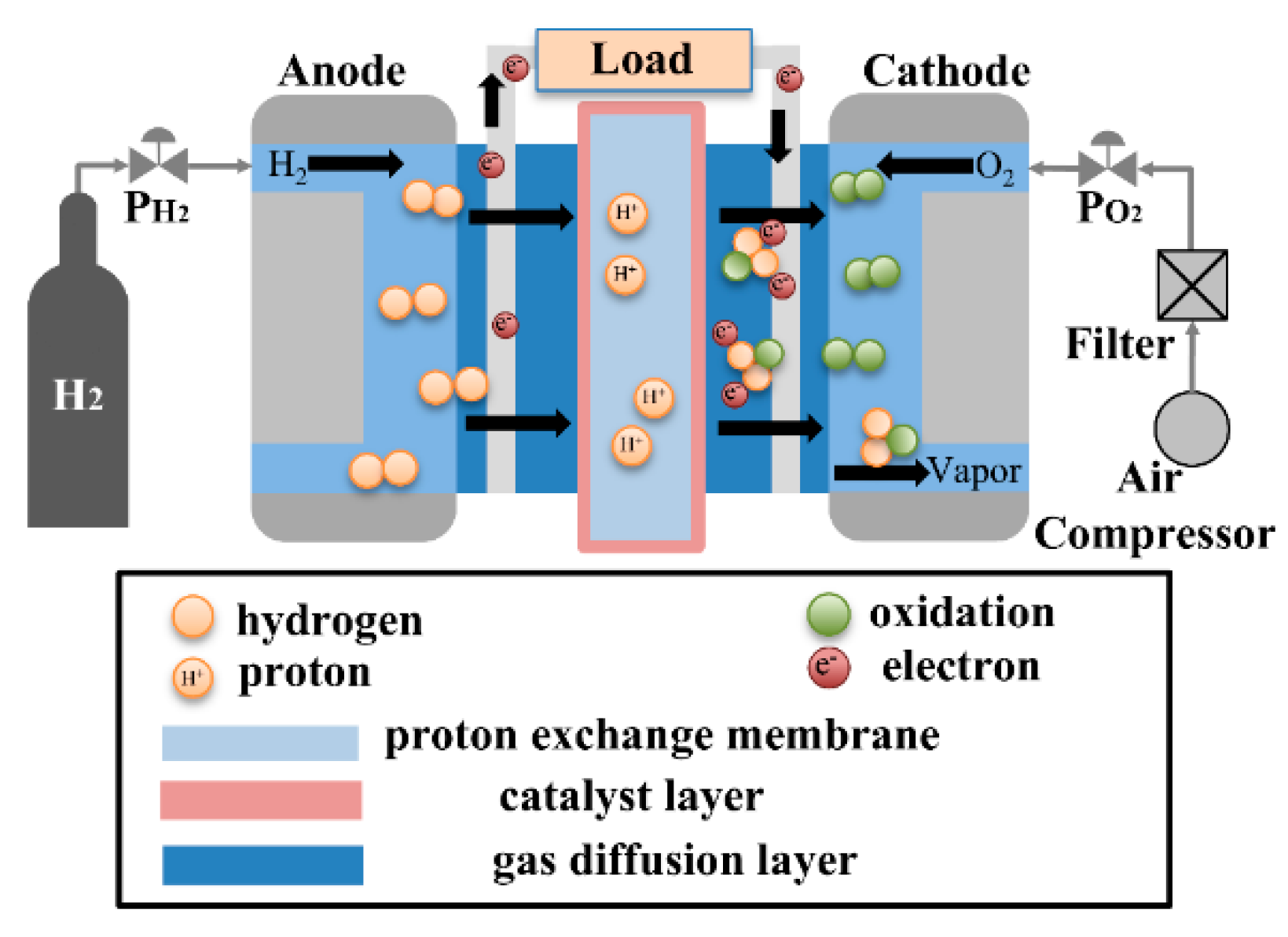
Figure 2.
(a)Diagram of spatial domains and their corresponding modeling[39]; (b)Typical polarization curve.
Figure 2.
(a)Diagram of spatial domains and their corresponding modeling[39]; (b)Typical polarization curve.
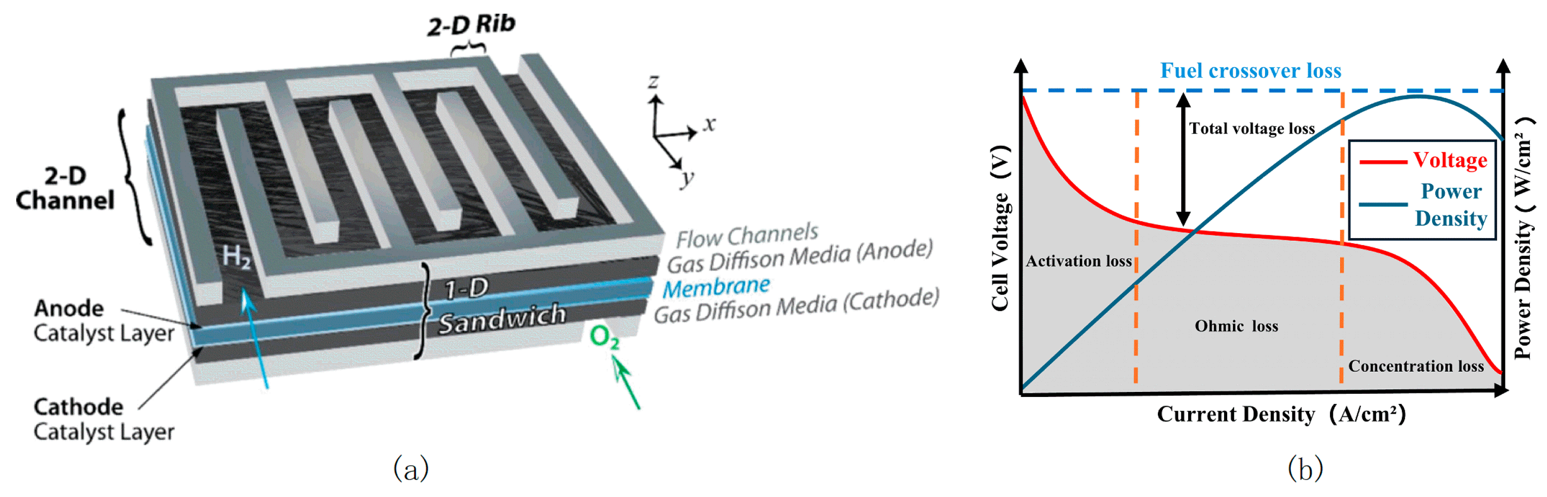
Figure 3.
The sequence of PEMFC modelling.
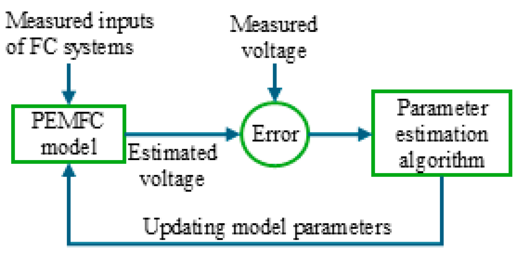
Table 3.
Overview of Commonly Used Objective Functions.
| Fitness function | Fundamental equations | Optimization Objective | |
| Sum of Squared Errors (SSE)[51] | Minimizing the sum of squared errors between predicted and observed values. | ||
| Mean square error (MSE)[52] | Minimize the average squared difference between predicted and observed values. | ||
| Root mean square error (RMSE)[46] | Minimize the square root of the mean squared error, reducing large prediction errors. | ||
| Normalized root mean square error (NRMSE)[53] | Measures error relative to the range or mean of observed values. | ||
| Absolute error (AE) [54] | Measures the absolute difference between predicted and observed values. | ||
| Mean absolute error (MAE)[48] | Evaluates the average of absolute differences between predicted and observed values. |
Table 4.
Fundamental features of different PEMFC types.
| PEMFCs’ type | Power (W) | N | A(cm2) | l (um) | Jmax (mA/cm2) | T(K) | (bar) | (bar) |
|---|---|---|---|---|---|---|---|---|
| Ballard Mark V [53] | 5000 | 35 | 50.6 | 178 | 1500 | 343 | 1 | 1 |
| SR-12 Modular[55] | 500 | 48 | 62.5 | 25 | 672 | 323 | 1.47628 | 0.2095 |
| NedStack PS 6KW[51] | 6000 | 65 | 240 | 178 | 937 | 343 | 0.5–5 | 0.5–5 |
| BCS 500W[47] | 500 | 32 | 64 | 178 | 469 | 333 | 1 | 0.2095 |
| 250W Stack[56] | 250 | 24 | 27 | 178 | 680 | 343 | 1 | 1 |
| Temasek 1 kW[57] | 1000 | 20 | 150 | 51 | 1500 | 323 | 0.5 | 0.5 |
| Horizon H-12[58] | 12 | 13 | 8.1 | 25 | 246.9 | 302.15 | 0.4935 | 1 |
| 30kw stack[59] | 30000 | 30 | 250 | 32 | 2.424 | 338.15 | 1.577 | 1.678 |
Table 5.
Typical limits of the unknown parameters.
| Parameter | Low | High |
|---|---|---|
| -1.1997 | -0.8532 | |
| ×10-3 | 1.00 | 5.00 |
| ×10-5 | 3.60 | 9.80 |
| ×10-5 | -26.00 | -9.54 |
| ×10-5 | 13.00 | 23.00 |
| 0.10 | 0.80 | |
| 0.0136 | 0.5000 |
Table 6.
PEMFC parameter estimation using Ballard-Mark-V dataset.
| Years | Methods | Parameters | SSE | ||||||
|---|---|---|---|---|---|---|---|---|---|
| ×10-3 | ×10-5 | ×10-4 | |||||||
| 2025 | IAGDE[64] | -0.8946 | 2.5300 | 3.6100 | -0.0009 | 3.56382 | 15200 | 0.0920 | 0.00104 |
| 2025 | PO[65] | -1.1997 | 3.5758 | 3.6000 | -1.6729 | 24.0000 | 1.0000 | 0.0159 | 0.81280 |
| 2025 | PO[66] | -0.9382 | 3.1690 | 8.3200 | -1.7000 | 14.4391 | 1.0000 | 0.0138 | 0.14860 |
| 2024 | FNN-POA[67] | -0.8851 | 2.7882 | 6.3684 | -1.7105 | 15.6807 | 5.1874 | 0.0168 | - |
| 2024 | RBMO[68] | -1.0006 | 3.8364 | 9.7953 | -1.6283 | 22.9999 | 1.0000 | 0.0136 | 0.85360 |
| 2024 | DACO[69] | -1.0950 | 3.4120 | 7.9310 | -0.9540 | 14.0800 | 0.8000 | 0.0182 | 0.00001 |
| 2024 | SHO[70] | -1.1993 | 3.6200 | 3.6704 | -1.7840 | 19.6862 | 3.0390 | 0.0665 | 0.00001 |
| 2023 | CBO[57] | -1.1788 | 2.8743 | 3.6400 | -1.1950 | 12.0800 | 8.0000 | 0.0136 | 0.00060 |
| 2023 | IAHA[71] | -1.0130 | 4.0000 | 8.9800 | -1.6300 | 23.0000 | 1.0000 | 0.0136 | 0.85360 |
| 2023 | ICSO[72] | -0.9600 | - | 4.2500 | -1.7000 | 23.0000 | 1.0000 | 0.0140 | 0.85300 |
| 2023 | ARO[73] | -1.1589 | 3.5208 | 4.0526 | -1.6725 | 23.9900 | 1.0000 | 0.0159 | 0.81391 |
| 2021 | ASSA[74] | -1.1100 | 3.1900 | 7.1700 | -1.5970 | 22.0000 | 1.0000 | 0.0110 | 0.82000 |
| 2019 | SSO[21] | -1.1827 | 3.7080 | 9.3600 | -1.1925 | 11.7603 | 7.8773 | 0.0136 | 0.00210 |
| 2019 | CS-EO[52] | -0.9728 | 3.4480 | 8.3832 | -1.1328 | 21.6995 | 8.0000 | 0.0136 | 0.00240 |
| 2019 | FPA[75] | -1.0257 | 3.4000 | 6.7952 | -1.2850 | 15.6446 | 5.2906 | 0.0614 | 0.00060 |
| 2019 | WOA[76] | -1.1978 | 4.4183 | 9.7214 | -1.6273 | 23.0000 | 1.0020 | 0.0136 | 0.02390 |
Disclaimer/Publisher’s Note: The statements, opinions and data contained in all publications are solely those of the individual author(s) and contributor(s) and not of MDPI and/or the editor(s). MDPI and/or the editor(s) disclaim responsibility for any injury to people or property resulting from any ideas, methods, instructions or products referred to in the content. |
© 2026 by the authors. Licensee MDPI, Basel, Switzerland. This article is an open access article distributed under the terms and conditions of the Creative Commons Attribution (CC BY) license (http://creativecommons.org/licenses/by/4.0/).
Copyright: This open access article is published under a Creative Commons CC BY 4.0 license, which permit the free download, distribution, and reuse, provided that the author and preprint are cited in any reuse.


