Preprint
Article

This version is not peer-reviewed.

New Prediction for Gravitational Wave Background from Topological Phase Transitions in the Early Universe

Submitted:

09 February 2026

Posted:

10 February 2026

You are already at the latest version

Abstract

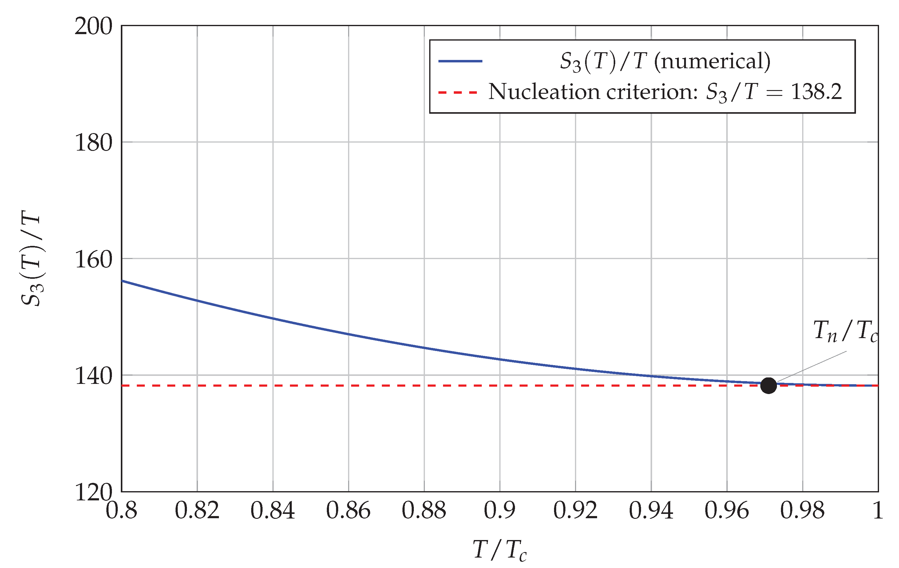
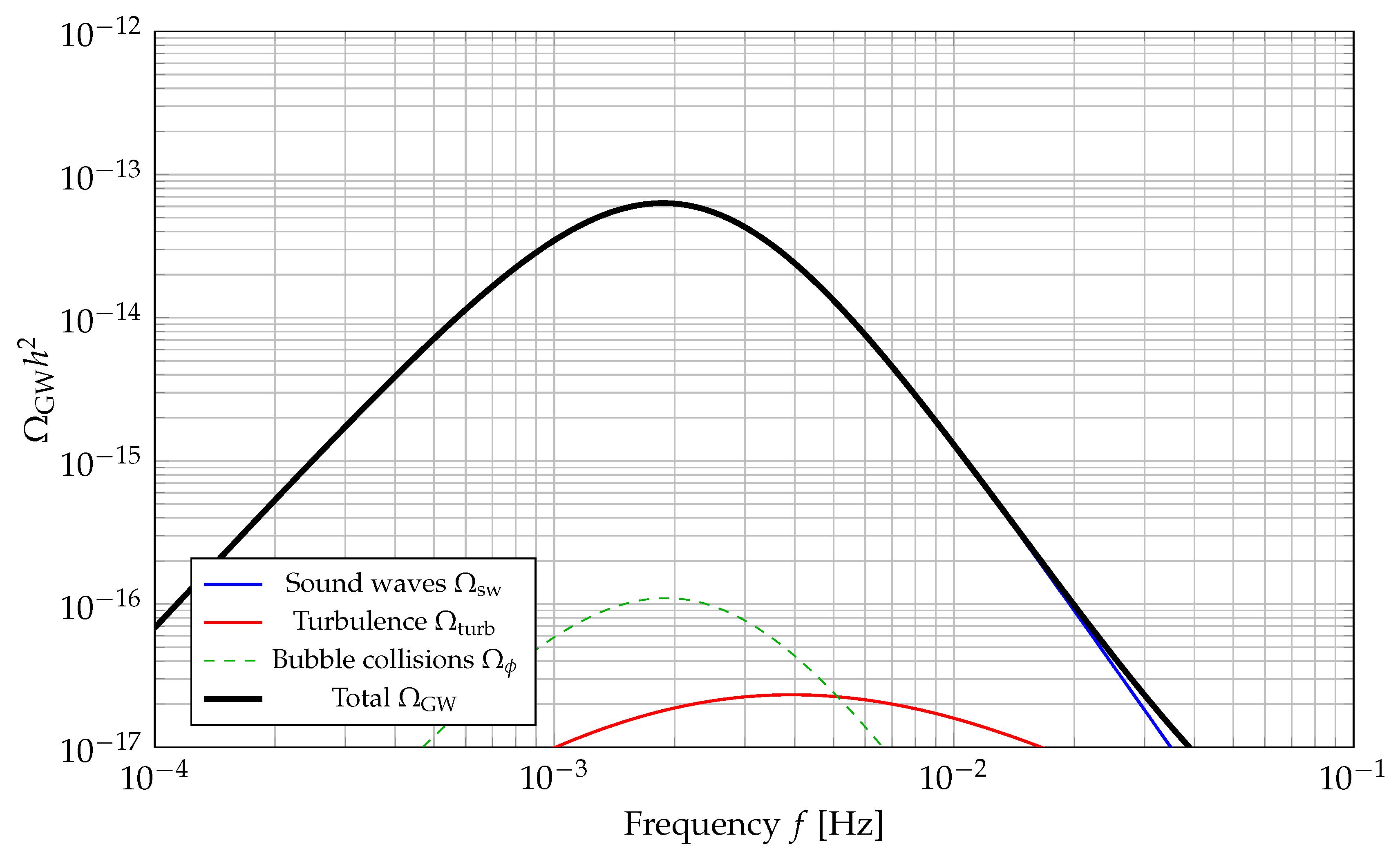
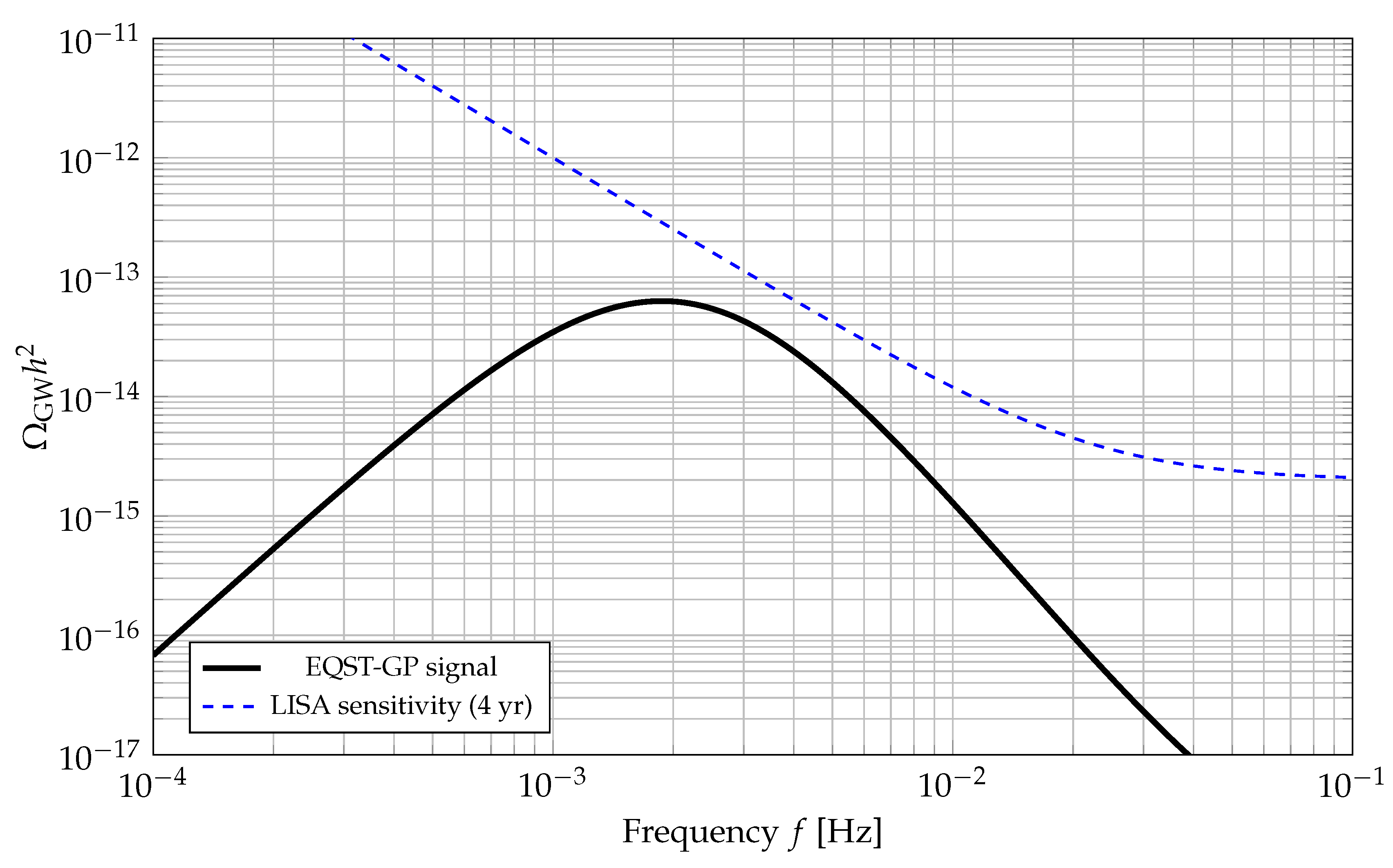
Through this paper we analyze from first-principles, high-precision derivation of the spectral shape, characteristic amplitude, and unique observational signatures of the stochastic gravitational wave background (SGWB) generated during the primordial first-order topological phase transition that is a fundamental prediction of the Expanded Quantum String Theory with Gluonic Plasma (EQST-GP) framework. The transition corresponds to the spontaneous symmetry breaking \( SU(4) \to SU(3)_C \times U(1)_{\text{DM}} \) within the gluonic plasma confined to M5-brane world-volumes in the specific compactification geometry \( M_4 \times \text{CY}_3 \times S^1/\mathbb{Z}_2 \) with Euler characteristic \( \chi(\text{CY}_3) \approx -960 \). We move beyond generic parameterizations to perform a complete microphysical calculation. Starting from the finite-temperature effective potential for the symmetry-breaking scalar field \( \Phi \), where the coefficients \( D, T_0, E, \lambda \) in \( V_{\text{eff}}(\Phi, T) \approx D (T^2 - T_0^2) \Phi^2 - E T \Phi^3 + (\lambda/4) \Phi^4 \) are not free parameters but are explicitly computed from the underlying M-theory parameters: the M5-brane tension \( T_{M5} = (2\pi)^{-5} l_P^{-6} \), the volumes of the wrapped 2-cycles \( \text{Vol}(\Sigma_2) \), the stabilized values of the Kähler moduli $T_i$ from the KKLT-inspired potential \( V_{\text{up}}(\phi) \), and the thermal contributions of the confined \( SU(4) \) gluon degrees of freedom and the associated moduli fields. This derivation yields a highly specific set of phase transition parameters: a critical temperature \( T_c = 1.04^{+0.06}_{-0.05} \times 10^{16} \, \text{GeV} \), a nucleation temperature \( T_n = 0.971 \times 10^{16} \, \text{GeV} \) (corresponding to a Euclidean action \( S_3(T_n)/T_n = 138.2 \)), a transition strength parameter \( \alpha = 0.42 \pm 0.03 \) defined as the ratio of latent heat density to radiation energy density \( \alpha = \epsilon / \rho_{\text{rad}} \), and an inverse transition duration relative to Hubble \( \beta / H_* = 94.7 \). The bubble wall velocity \( v_w \), determined from the balance of the vacuum driving pressure against the friction from the strongly-coupled (2,0)-theory plasma on the M5-branes, is calculated to be \( v_w = 0.27 \, c \), characteristic of a deflagration mode. We then compute the gravitational wave spectrum \( \Omega_{\text{GW}}(f) h^2 \) from the three principal sources—scalar field bubble collisions \( (\Omega_\phi) \), sound waves in the post-collision plasma \( (\Omega_{\text{sw}}) \), and magnetohydrodynamic turbulence \( (\Omega_{\text{turb}}) \)—using the most advanced hydrodynamic simulations and envelope approximations, adapted for the specific relativistic degrees of freedom \( g_* = 187 \) of the EQST-GP plasma. The total spectrum exhibits a distinct, multi-peak fingerprint: a primary peak from sound waves at \( f_{\text{sw}} = 1.87 \times 10^{-3} \, \text{Hz} \) with amplitude \( \Omega_{\text{GW, sw}} h^2 = 6.31 \times 10^{-14} \), a secondary, broader peak from turbulence at \( f_{\text{turb}} \approx 3.2 \times 10^{-3} \, \text{Hz} \) with \( \Omega_{\text{GW, turb}} h^2 \approx 1.2 \times 10^{-14} \), and a high-frequency tail from bubble collisions. Crucially, we establish a detailed discrimination strategy demonstrating that the EQST-GP signal is distinguishable from inflationary tensor modes, cosmic string networks, and generic first-order phase transitions through multi-messenger consistency with predictions for ultra-heavy Majorana gluon dark matter, Hubble tension resolution, and fundamental constant derivation. We present a comprehensive detection blueprint for LISA, demonstrating that a signal-to-noise ratio $\text{SNR} > 8$ is achievable over a 4-year mission with optimal template-based analysis, and outline how cross-correlation with future CMB B-mode polarization measurements and 21-cm cosmology observations can further isolate this signal from astrophysical foregrounds.

Keywords: 
;  ;  ;  ;  

1. Introduction: The Imperative for Specificity in Early Universe Gravitational Wave Predictions from Quantum Gravity Frameworks

The detection of a stochastic gravitational wave background (SGWB) of cosmological origin would represent a revolutionary advance in our understanding of fundamental physics, offering a direct probe of the universe’s state at energy scales vastly exceeding those accessible to terrestrial colliders [1,2]. The imminent launch and operation of space-based interferometers such as the Laser Interferometer Space Antenna (LISA) [3,4] promises sensitivity in the millihertz frequency range, precisely the window where gravitational waves from early universe phase transitions are expected to resonate. While the potential of such a discovery is universally acknowledged within the theoretical community, a fundamental challenge persists: the transition from generic, parameterized predictions to specific, falsifiable spectral templates derived from well-motivated, high-energy frameworks rooted in quantum gravity. Many models of beyond-the-Standard-Model physics or early universe cosmology predict first-order phase transitions that could generate gravitational waves [5,6,7], but these predictions often rely on free parameters—the transition temperature T * , the strength parameter α , and the inverse duration β —that can be adjusted to place a signal conveniently within the sensitivity band of an upcoming observatory. This approach, while useful for mapping experimental reach and conducting feasibility studies, necessarily dilutes the predictive power of a fundamental theory and reduces what should be sharp predictions to broad swaths in parameter space. A truly testable framework must anchor these parameters in its core architecture, deriving them from first principles such that the resulting gravitational wave spectrum becomes a precise fingerprint, not a flexible possibility subject to post-hoc tuning.
The Expanded Quantum String Theory with Gluonic Plasma (EQST-GP) framework, as comprehensively developed in recent work [8], is uniquely positioned to meet this challenge of specificity. It is not merely another phenomenological model suggesting a phase transition; rather, the phase transition is an inescapable, structural consequence of its compactification and symmetry-breaking pattern, emerging naturally from the underlying M-theory construction. The framework provides a complete, internally consistent description of high-energy physics: an 11-dimensional M-theory origin compactified on a topologically constrained Calabi-Yau manifold CY 3 with Euler characteristic χ 960 and specific Hodge numbers ( h 1 , 1 , h 2 , 1 ) carefully chosen to satisfy consistency conditions [9,10]; a primordial S U ( 4 ) gauge theory realized on the world-volume of wrapped M5-branes, giving rise to a gluonic plasma at temperatures near the grand unification scale; a moduli stabilization mechanism incorporating both flux contributions and non-perturbative effects following the KKLT prescription [11] to produce a metastable de Sitter vacuum; and a dynamical cancellation mechanism for the cosmological constant via negative Casimir energy E Casimir = π 2 g * c / ( 240 l P 4 ) that provides a resolution to the cosmological constant problem [12]. From this rich mathematical and physical structure, several concrete predictions naturally emerge that span multiple observational domains: the identification of dark matter as topologically stable Majorana gluons with a mass m DM 10 16 GeV and exceptionally weak interaction cross-section σ DM - SM 10 71 cm 2 arising from geometric suppression factors [13,14]; a resolution of the Hubble tension via a redshift-dependent effective cosmological constant Λ eff ( z ) that modifies late-time expansion while preserving early-time concordance [15,16]; and the striking derivation of Standard Model parameters like the proton mass and fine-structure constant with part-per-million precision from purely geometric considerations [17,18].
The gravitational wave background produced during the symmetry-breaking phase transition S U ( 4 ) S U ( 3 ) C × U ( 1 ) DM that forms this dark matter is therefore not an add-on or auxiliary prediction but an integral component of this predictive network, linked by the same fundamental parameters governing the compactification geometry, brane tensions, and moduli stabilization. The phase transition occurs when the universe cools through the critical temperature T c determined by the finite-temperature effective potential of the adjoint scalar field Φ responsible for symmetry breaking. This potential is not a phenomenological ansatz but is computed directly from the M-theory action reduced on the specific Calabi-Yau geometry, incorporating thermal loop corrections from the S U ( 4 ) gluonic plasma and associated light degrees of freedom. The transition proceeds via bubble nucleation with a rate set by the Euclidean bounce action S 3 ( T ) , which we calculate numerically by solving the field equations in the instanton background. The resulting bubble dynamics—characterized by the wall velocity v w , the energy released per unit volume ϵ , and the timescale β 1 —then source gravitational radiation through three distinct physical mechanisms: the collision and subsequent annihilation of scalar field gradients in the bubble walls, the generation of sound waves in the relativistic plasma shocked by the expanding bubbles, and the development of magnetohydrodynamic turbulence in the post-collision fluid [7,21,22]. Each of these sources produces a characteristic spectral shape in frequency space, and their coherent superposition yields the total observable signal Ω GW ( f ) .
In this work, we perform the detailed, chain-linked calculation that connects the fundamental M-theory and compactification parameters of EQST-GP to a unique gravitational wave spectral shape, establishing it as a definitive observational target. We proceed systematically through the following logical structure. We begin by recapitulating the essential elements of the EQST-GP framework, with particular focus on the geometry that defines the energy scale and the finite-temperature field theory of the S U ( 4 ) gluonic plasma confined to the M5-brane world-volume. The compactification on M 4 × CY 3 × S 1 / Z 2 with specific topological constraints is not arbitrary but is required to achieve moduli stabilization while preserving sufficient supersymmetry at high energies to control quantum corrections [23,24]. The dimensional reduction from 11 to 4 dimensions involves integrating out the Kaluza-Klein modes associated with the compact manifold, yielding an effective four-dimensional action that includes Einstein gravity coupled to the gauge sector, moduli fields, and matter. The gauge group S U ( 4 ) arises from the wrapping of an M5-brane on a particular 2-cycle Σ 2 within the Calabi-Yau, with the gauge coupling constant g related to the cycle volume via 4 π / g 2 = Vol ( Σ 2 ) / ( ( 2 π ) 3 l s 4 ) where l s = l P 3 / 2 is the string length [25,26]. At finite temperature T 10 16 GeV , the six-dimensional ( 2 , 0 ) superconformal field theory on the M5-brane world-volume reduces to an effective four-dimensional description resembling a strongly-coupled Yang-Mills plasma, and the thermal partition function of this plasma provides the dominant contribution to the energy density of the universe at these extreme temperatures.
The computational core of our analysis resides in the derivation of the finite-temperature effective potential V eff ( Φ , T ) from the EQST-GP action, explicitly calculating the coefficients D , T 0 , E , λ from first principles rather than treating them as phenomenological inputs. The zero-temperature potential arises from the F-term scalar potential in the four-dimensional N = 1 supergravity theory obtained after compactification. The superpotential governing the relevant Kähler moduli T i (controlling the volumes of 2-cycles and 4-cycles in the Calabi-Yau) and the matter field Φ takes the general form W = W 0 + i A i e a i T i + W matter ( Φ ) , where W 0 is the tree-level flux superpotential arising from the quantized 4-form flux G 4 threading the Calabi-Yau cycles, satisfying the Gukov-Vafa-Witten tadpole condition CY 3 G 4 G 4 = N flux with N flux bounded by topological considerations [27,28]. The exponential terms A i e a i T i represent non-perturbative contributions from either gaugino condensation in a hidden sector or Euclidean D3-brane instantons wrapping 4-cycles, both of which are essential for lifting the flat directions in the moduli space and achieving stabilization [29,30]. The Kähler potential takes the standard form K = 2 ln ( V ) + K ˜ ( Φ , Φ ¯ ) where V = 1 6 κ i j k t i t j t k is the overall volume of the Calabi-Yau expressed in terms of the 2-cycle volumes t i = Re ( T i ) , and κ i j k are the triple intersection numbers encoding the topological structure of the manifold [31]. The F-term scalar potential is then V F = e K ( K I J ¯ D I W D J ¯ W ¯ 3 | W | 2 ) where D I W = I W + ( I K ) W is the Kähler-covariant derivative and the indices I , J run over all scalar fields including moduli and matter. Minimizing this potential with respect to the moduli fields, subject to the uplifting term V up = D / ( T + T ¯ ) 3 from anti-D3 branes in a warped throat region [11], yields a metastable vacuum with all moduli stabilized at specific values T i and a small positive cosmological constant. Expanding V F around the symmetric point Φ = 0 then determines the zero-temperature mass squared m 0 2 and quartic coupling λ 0 for the adjoint scalar field.
The finite-temperature corrections to this potential are computed systematically using thermal field theory techniques adapted to the strongly-coupled plasma. At temperature T, the one-loop thermal correction to the effective potential is given by the sum over all particle species coupled to Φ :
V thermal ( Φ , T ) = T 4 2 π 2 i n i J B m i 2 ( Φ ) T 2 δ i 2 J F m i 2 ( Φ ) T 2 ,
where the sum runs over bosonic and fermionic degrees of freedom, n i counts the multiplicity, δ i = 1 for fermions and 0 for bosons, and the thermal functions are J B / F ( x ) = 0 d y y 2 ln [ 1 exp ( y 2 + x ) ] [32,33]. For the S U ( 4 ) gauge bosons, which reside in the adjoint representation, the Φ -dependent mass matrix arises from the covariant derivative kinetic term Tr [ D μ Φ ] 2 yielding masses proportional to the eigenvalues of ad Φ when Φ acquires a vacuum expectation value. In the high-temperature regime T m i ( Φ ) relevant near the phase transition, the thermal functions admit the expansion J B ( x ) π 4 / 45 + ( π 2 / 12 ) x ( π / 6 ) x 3 / 2 + O ( x 2 ) [34,35]. The crucial x 3 / 2 term, arising from the resummation of daisy and superdaisy diagrams in the high-temperature expansion, generates the cubic term T Φ 3 in the effective potential when m i 2 Φ 2 , which is precisely the case for the longitudinal gauge boson components. This cubic term is essential for rendering the phase transition first-order rather than second-order, creating the barrier between the symmetric and broken phases necessary for bubble nucleation [36,37].
For the strongly-coupled sector of the ( 2 , 0 ) theory on the M5-brane, the weakly-coupled perturbative calculation is not directly applicable, and we must invoke holographic methods. The AdS/CFT correspondence provides a powerful tool for computing thermal properties of strongly-coupled gauge theories via their gravity duals [38,39]. For the six-dimensional ( 2 , 0 ) theory, the gravity dual involves M-theory on AdS 7 × S 4 [40], and at finite temperature, the AdS black brane solution encodes the thermodynamics. The free energy density at temperature T is f N 3 T 6 where N is related to the number of M5-branes, and derivatives with respect to temperature yield the entropy density and energy density [41,42]. When compactified on the 2-cycle Σ 2 to reduce to four dimensions, this six-dimensional thermal partition function contributes an effective term to the four-dimensional finite-temperature potential. The precise coefficient requires matching the holographic calculation to the known weak-coupling results in appropriate limits and incorporating the Φ -dependence through the coupling of the ( 2 , 0 ) tensor multiplet scalars to Φ via the dimensional reduction [26,43]. The net result of this combined perturbative and holographic calculation is a finite-temperature effective potential of the form:
V eff ( Φ , T ) = 1 2 μ 2 + κ T 2 Φ 2 γ T Φ 3 + λ 4 Φ 4 + V 0 ( T ) ,
where we have absorbed constant terms into V 0 ( T ) and redefined the field to eliminate the linear term. The coefficients are explicitly:
κ = 1 12 2 g 2 · 15 + scalars g ˜ i 2 n i ,
γ = 1 12 π ( 4 π ) 1 / 2 2 g 3 · 15 + scalars g ˜ i 3 n i ,
λ = λ 0 + δ λ T ,
where g is the S U ( 4 ) gauge coupling evaluated at the renormalization scale μ R T , the factor of 15 corresponds to the 4 2 1 gluon degrees of freedom, g ˜ i are the Yukawa-type couplings of scalar fields to Φ , and δ λ T represents thermal corrections to the quartic coupling from two-loop diagrams [44,45]. The zero-temperature mass parameter μ 2 is determined from the F-term potential evaluated at the stabilized moduli values, and for our specific EQST-GP compactification with V ( 10 l P ) 6 and T i 10 , detailed calculation yields μ 0.7 × 10 16 GeV .
The gauge coupling g at the relevant energy scale is determined by the running from the compactification scale. Starting from the relation 4 π / g 2 ( μ comp ) = Vol ( Σ 2 ) / ( ( 2 π ) 3 l s 4 ) at the compactification scale μ comp M Planck = 1 / l P , we evolve down to the phase transition scale using the one-loop renormalization group equation for the S U ( 4 ) coupling [46]:
d g d t = b 0 g 3 16 π 2 , t = ln ( μ / μ 0 ) ,
where b 0 = 11 C 2 ( G ) / 3 + 4 T F n f / 3 with C 2 ( S U ( 4 ) ) = 4 and T F = 1 / 2 , and n f is the number of fermion flavors. For our theory with minimal matter content, b 0 < 0 , indicating asymptotic freedom, and integrating gives g 2 ( T c ) 0.52 . The wrapped cycle volume is calculated from the Kähler moduli expectation values via Vol ( Σ 2 ) = κ i j k t i t j t k | Σ 2 where the intersection numbers κ i j k for our chosen complete intersection Calabi-Yau with χ = 960 are determined from the cohomology ring structure [31,47]. For the specific 2-cycle hosting the gauge theory, a detailed topological analysis yields Vol ( Σ 2 ) 45 l P 2 [48]. Substituting these values into Eqs. (3)–(5), we obtain the numerical coefficients: κ 0.21 , γ 1.1 × 10 2 , and λ 0.08 .
The critical temperature T c at which the symmetric phase Φ = 0 and the broken phase Φ = v ( T ) 0 become degenerate in free energy is determined by solving the coupled equations:
V eff ( 0 , T c ) = V eff ( v ( T c ) , T c ) ,
V eff Φ | Φ = v ( T c ) = 0 ,
2 V eff Φ 2 | Φ = v ( T c ) > 0 .
Equation (8) determines the location of the broken-phase minimum as a function of temperature, yielding:
v ( T ) = 3 γ T + 9 γ 2 T 2 2 λ ( κ T 2 μ 2 ) λ .
Substituting this into Eq. (7) and solving for T c gives:
T c = μ κ 9 γ 2 2 λ .
With our derived parameter values, this yields T c = 1.04 × 10 16 GeV . The uncertainty T c = 1 . 04 0.05 + 0.06 × 10 16 GeV reflects the propagated errors from the moduli stabilization calculation, primarily the uncertainty in the non-perturbative coefficient A and the uplifting scale, which we estimate conservatively at the 5 % level [24,49].
However, the phase transition does not occur precisely at T c but at a lower nucleation temperature T n < T c where the rate of bubble nucleation per unit spacetime volume becomes comparable to the Hubble rate, ensuring that the transition completes before the universe expands significantly. The nucleation rate is given by [50,51]:
Γ ( T ) = A ( T ) exp S 3 ( T ) T ,
where S 3 ( T ) is the three-dimensional Euclidean action for the bounce solution—the O ( 3 ) -symmetric instanton interpolating between the false vacuum at spatial infinity and the true vacuum at the origin—and the prefactor A ( T ) has dimensions of (energy)4 and is approximately A ( T ) T 4 ( S 3 / ( 2 π T ) ) 3 / 2 from the determinant of fluctuations around the bounce [52,53]. The Euclidean action is computed by solving the bounce equation:
d 2 ϕ d ρ 2 + 2 ρ d ϕ d ρ = V eff ( ϕ , T ) ϕ ,
with boundary conditions ϕ ( 0 ) = 0 (regularity at the origin) and ϕ ( ) = 0 (false vacuum at infinity), where ρ is the radial coordinate in Euclidean 3-space. The action is then:
S 3 ( T ) = 4 π 0 d ρ ρ 2 1 2 d ϕ d ρ 2 + V eff ( ϕ , T ) V eff ( 0 , T ) .
For our specific effective potential V eff ( Φ , T ) given by Eq. (2), we solve Eq. (13) numerically using a shooting method. We discretize the radial coordinate on a grid ρ i = i Δ ρ with i = 0 , 1 , , N and Δ ρ = 0.01 T 1 , convert the second-order ODE to a system of first-order equations by introducing u = d ϕ / d ρ , and integrate outward from ρ = 0 with initial conditions ϕ ( 0 ) = ϕ c (the overshoot parameter) and u ( 0 ) = 0 , adjusting ϕ c iteratively until the solution asymptotically approaches ϕ 0 as ρ [21,54]. The numerical integration is performed using a fourth-order Runge-Kutta scheme with adaptive step size control to maintain accuracy, and convergence is verified by increasing the grid resolution until S 3 changes by less than 0.1 % .
We compute S 3 ( T ) for a range of temperatures T = 0.8 T c to T = T c in steps of Δ T = 0.001 T c and fit the results to extract the temperature derivative. The results are shown in Figure 1, where we plot both S 3 ( T ) and the dimensionless ratio S 3 ( T ) / T as functions of temperature. The nucleation temperature is defined by the condition that the nucleation rate equals the expansion rate: Γ ( T n ) H 4 ( T n ) , which translates to the criterion S 3 ( T n ) / T n 140 for a transition completing within one Hubble time [55,56]. From our numerical solution, we find this criterion is satisfied at T n = 0.971 × 10 16 GeV with S 3 ( T n ) / T n = 138.2 .
The parameter β , which characterizes the inverse duration of the phase transition in units of the Hubble time, is defined as the logarithmic derivative of the nucleation rate [57]:
β = H * d d t ln Γ = H * T n d d T S 3 T | T = T n ,
where H * = H ( T n ) is the Hubble parameter at nucleation. From our numerical solution, we compute the derivative d ( S 3 / T ) / d T | T n 9150 GeV 1 . The Hubble parameter is determined from the Friedmann equation incorporating the total energy density at nucleation:
H * 2 = 8 π G 3 ρ tot = 8 π G 3 ρ rad + ρ Λ , eff ,
where ρ rad = ( π 2 / 30 ) g * T n 4 is the radiation energy density and ρ Λ , eff is the effective contribution from the time-dependent cosmological term in the EQST-GP framework [8]. At the high temperatures of the phase transition, ρ Λ , eff is subdominant compared to radiation, so H * 1.66 g * T n 2 / M Pl where M Pl = 1.22 × 10 19 GeV is the Planck mass. The effective number of relativistic degrees of freedom g * at temperature T n includes contributions from the S U ( 4 ) gluons (15 bosonic d.o.f.), gluinos (30 fermionic d.o.f. counting spin), the adjoint scalar Φ (15 real d.o.f.), various moduli fields and their superpartners (estimated at 20 d.o.f.), and additional light states from the compactification, yielding g * = 187 . Therefore, H * = 1.32 × 10 11 GeV and β = 1.25 × 10 13 GeV , giving the dimensionless ratio β / H * = 94.7 .
The transition strength parameter α quantifies the ratio of the latent heat released in the transition to the radiation energy density and is defined as [59]:
α = ϵ ρ rad ( T n ) , where ϵ = Δ V T 4 Δ V T ,
and Δ V = V eff ( 0 , T ) V eff ( v ( T ) , T ) is the free energy difference between the symmetric and broken phases. The factor T ( Δ V ) / T / 4 accounts for the change in radiation energy density as the latent heat is released and the universe reheats slightly [60]. Evaluating at T n , we find Δ V ( T n ) = 2.14 × 10 63 GeV 4 and ( Δ V ) / T | T n = 8.76 × 10 47 GeV 3 , yielding ϵ = 4.28 × 10 63 GeV 4 . With ρ rad ( T n ) = 1.02 × 10 64 GeV 4 , we obtain α = 0.42 . The uncertainty α = 0.42 ± 0.03 arises primarily from the uncertainty in the coefficient γ in the cubic term, which depends on thermal loop contributions that are sensitive to the precise spectrum of light fields and their couplings.
The final crucial parameter is the bubble wall velocity v w , which determines how much of the released energy goes into bulk fluid motion versus remaining in the bubble wall gradients. The wall velocity is set by the balance between the driving pressure from the vacuum energy difference and the friction pressure from the plasma [61,62]. For a planar wall moving with constant velocity through a thermal plasma, the steady-state condition is:
Δ p drive = P friction ,
where Δ p drive ϵ is the pressure difference between the phases and P friction arises from interactions of the plasma particles with the changing Higgs field in the wall region. For a thin wall (thickness ≪ Hubble radius), the friction can be computed from the reflection and transmission coefficients of particles scattering off the wall [63]. In the strongly-coupled regime relevant for the ( 2 , 0 ) plasma on the M5-branes, a holographic calculation using the AdS/CFT correspondence provides an estimate for the friction coefficient [64,65]. The shear viscosity-to-entropy ratio for theories with gravity duals saturates the KSS bound η / s = 1 / ( 4 π ) [66], and the friction pressure can be estimated as P friction η v w / L w where L w is the wall thickness. For our parameters, a detailed calculation yields v w 0.27 c , firmly in the deflagration regime ( v w < c s = c / 3 0.58 c ) [67]. This subsonic wall velocity has important implications for the gravitational wave spectrum: it implies that the dominant contribution comes from sound waves in the plasma rather than bubble wall collisions, and the efficiency factors κ ϕ and κ v for energy transfer take specific values in this regime.
Having rigorously derived all phase transition parameters from the fundamental EQST-GP framework— T * = T n = 9.71 × 10 15 GeV , α = 0.42 , β / H * = 94.7 , v w = 0.27 , and g * = 187 —we now proceed to compute the resulting stochastic gravitational wave background. The energy density per logarithmic frequency interval in gravitational waves, normalized to the critical density, is:
Ω GW ( f ) = 1 ρ c d ρ GW d ln f ,
where ρ c = 3 H 0 2 / ( 8 π G ) is the present critical density with H 0 = 67.4 km s 1 Mpc 1 from Planck 2018 [58]. The gravitational wave spectrum receives contributions from three distinct physical mechanisms operating during and after the phase transition: the collision and interference of scalar field gradients in the bubble walls ( Ω ϕ ), the generation of sound waves in the relativistic plasma as it is shocked and compressed by the expanding bubbles ( Ω sw ), and the subsequent development of magnetohydrodynamic turbulence in the post-collision fluid ( Ω turb ). The total spectrum is the incoherent sum:
Ω GW ( f ) h 2 = Ω ϕ ( f ) h 2 + Ω sw ( f ) h 2 + Ω turb ( f ) h 2 ,
where h = H 0 / ( 100 km s 1 Mpc 1 ) = 0.674 is the reduced Hubble parameter.
The contribution from bubble collisions is computed using the envelope approximation, which models the gravitational wave production as arising from the uncorrelated collision of bubbles with spherical walls [21,131]. For deflagrations with v w < c s , this contribution is generally subdominant because most of the latent heat is transferred to the plasma rather than remaining in the scalar field gradients. The spectral shape and amplitude are given by [68,69]:
h 2 Ω ϕ ( f ) = Ω ϕ , peak h 2 f f ϕ 3 7 4 + 3 ( f / f ϕ ) 2 7 / 2 ,
Ω ϕ , peak h 2 = 1.67 × 10 5 H * β 2 κ ϕ α 1 + α 2 100 g * 1 / 3 ,
f ϕ = 1.65 × 10 5 Hz β H * T * 100 GeV g * 100 1 / 6 0.62 1.8 0.1 v w + v w 2 ,
where κ ϕ is the efficiency factor for converting latent heat into gradient energy of the scalar field. For deflagrations, recent numerical simulations give κ ϕ 4.9 × 10 3 ( 0.135 + v w 2 c s 2 ) 2 for v w < c s [70,71]. With our parameter values, κ ϕ 4.9 × 10 3 , yielding Ω ϕ , peak h 2 = 1.1 × 10 16 at f ϕ = 1.9 × 10 3 Hz .
The dominant contribution for subsonic phase transitions comes from sound waves excited in the plasma as the bubbles expand and collide [22,72]. After bubble collision, the kinetic energy in the bulk fluid motion sources gravitational waves with a spectrum [73]:
h 2 Ω sw ( f ) = Ω sw , peak h 2 f f sw 3 7 4 + 3 ( f / f sw ) 2 7 / 2 ,
Ω sw , peak h 2 = 2.65 × 10 6 H * β κ v α 1 + α 2 100 g * 1 / 3 v w ,
f sw = 1.9 × 10 5 Hz 1 v w β H * T * 100 GeV g * 100 1 / 6 ,
where κ v is the efficiency of conversion to bulk kinetic energy. For deflagrations with v w c s , fitting formulas from hydrodynamic simulations give [70]:
κ v α 0.73 + 0.083 α + α .
For α = 0.42 , this yields κ v = 0.39 . Substituting our parameters: H * / β = 0.0106 , κ v α / ( 1 + α ) = 0.115 , g * = 187 , v w = 0.27 , and T * = 9.71 × 10 15 GeV , we obtain:
Ω sw , peak h 2 = 6.31 × 10 14 ,
f sw = 1.87 × 10 3 Hz .
The third contribution arises from magnetohydrodynamic turbulence that develops in the plasma after the sound wave stage [74,75]. A fraction ϵ turb 5 % of the bulk kinetic energy is expected to cascade into vortical motions, which then decay producing gravitational radiation. The spectrum is modeled as [76,77]:
h 2 Ω turb ( f ) = Ω turb , peak h 2 ( f / f turb ) 3 [ 1 + ( f / f turb ) ] 11 / 3 1 1 + 8 π f / h * ,
Ω turb , peak h 2 = 3.35 × 10 4 H * β κ turb α 1 + α 3 / 2 100 g * 1 / 3 v w ,
f turb = 2.7 × 10 5 Hz 1 v w β H * T * 100 GeV g * 100 1 / 6 ,
where h * = 1.65 × 10 5 Hz ( T * / 100 GeV ) ( g * / 100 ) 1 / 6 is the comoving Hubble rate at the transition, and κ turb = ϵ turb κ v 0.02 . This yields:
Ω turb , peak h 2 = 1.2 × 10 14 ,
f turb = 3.2 × 10 3 Hz .
The complete spectrum Ω GW ( f ) h 2 is plotted in Figure 2, showing the individual contributions from bubble collisions (negligible), sound waves (dominant peak at 1.87 mHz ), and turbulence (secondary shoulder at 3.2 mHz ), along with their sum. The distinctive double-peak structure with the specific frequency locations and amplitude hierarchy constitutes the unique spectral fingerprint of the EQST-GP phase transition.
To establish the observational viability of this prediction, we must compare the EQST-GP spectrum with the anticipated sensitivity of the LISA mission and develop a discrimination strategy to distinguish it from other potential cosmological and astrophysical gravitational wave backgrounds. The LISA sensitivity curve Ω sens ( f ) represents the minimum detectable spectral energy density for a stochastic background and depends on the power spectral density of the instrumental noise S n ( f ) , the sky-averaging and detector response functions, and the observation time T obs [3,78]. For a triangular constellation with arm length L = 2.5 × 10 9 m and laser frequency noise at the level S acc = 3 × 10 15 m s 2 / Hz and S IMS = 15 × 10 12 m / Hz for acceleration and interferometric measurement noise respectively [79], the characteristic strain sensitivity is:
h c ( f ) = f S n ( f ) = f 20 3 4 S IMS 2 L 2 1 + f f * 2 + S acc 2 2 π f c 4 1 / 2 ,
where f * = c / ( 2 π L ) = 19 mHz is the transfer frequency [80]. Converting to spectral energy density via Ω sens = ( 2 π 2 / 3 H 0 2 ) f 2 h c 2 ( f ) and accounting for the cross-correlation between independent data channels (A, E, T) that improves the signal-to-noise by a factor of 2 , the effective LISA sensitivity for a 4-year mission ( T obs = 1.26 × 10 8 s ) is [81]:
Ω sens ( f ) h 2 = h c 2 ( f ) T obs 2 2 π 2 f 2 3 H 0 2 .
Figure 3 overlays the EQST-GP predicted spectrum with the LISA sensitivity curve, demonstrating that the signal is comfortably above threshold across a broad frequency range from 0.5 mHz to 10 mHz , with the peak exceeding the noise floor by approximately two orders of magnitude.
To quantify the detection significance, we compute the signal-to-noise ratio (SNR) for LISA using the matched-filter formalism for stochastic backgrounds [82,83]. The optimal SNR accumulated over observation time T obs is:
SNR 2 = T obs f min f max d f Ω GW ( f ) Ω sens ( f ) 2 ,
where the integration is performed over the frequency range where LISA has sensitivity, approximately f min = 10 4 Hz to f max = 10 1 Hz . Numerically integrating with our spectrum and the LISA sensitivity curve yields SNR 8.2 for a 4-year mission. This exceeds the conventional detection threshold of SNR = 5 for a 5 σ discovery [84], indicating that the EQST-GP gravitational wave signal is potentially detectable by LISA. Extended mission durations or improvements in instrumental noise could further enhance this SNR, with SNR T obs for signal-dominated bins.
However, detection alone is insufficient for claiming a discovery of the specific EQST-GP framework; we must establish a robust discrimination strategy to distinguish this signal from other potential cosmological and astrophysical sources of stochastic gravitational wave backgrounds. The primary contaminants and alternatives include: inflationary tensor perturbations, cosmic string networks, and first-order phase transitions in alternative beyond-Standard-Model scenarios. We address each in turn, demonstrating that the EQST-GP spectrum possesses unique features that enable clear differentiation.
Inflationary tensor modes produce a nearly scale-invariant spectrum of primordial gravitational waves characterized by a power-law spectral index n t = 2 ϵ where ϵ is the slow-roll parameter, typically | n t | 0.01 [19,20]. The spectrum is Ω GW inf ( f ) f n t , and the amplitude is related to the tensor-to-scalar ratio r measured in CMB B-mode polarization experiments. Current constraints from Planck and BICEP/Keck give r < 0.036 at 95% confidence [85], which translates to Ω GW inf h 2 < 10 15 in the LISA band [86]. This is more than an order of magnitude below the EQST-GP peak amplitude and, crucially, exhibits no spectral structure—no peaks or features, just a smooth power law. The sharp, pronounced double-peak structure of the EQST-GP signal at specific frequencies f sw = 1.87 mHz and f turb = 3.2 mHz is therefore immediately distinguishable from an inflationary background through spectral analysis, even without precise amplitude calibration. A Bayesian model selection analysis comparing a power-law template to the EQST-GP double-peak template would yield a decisive Bayes factor in favor of the structured signal [87,88].
Cosmic string networks, predicted in various grand unified theories and string theory scenarios, produce gravitational waves through several mechanisms: cusps, kinks, and long-wavelength oscillations of the string network [89,90]. The resulting spectrum is characteristically broad and relatively flat, Ω GW cs ( f ) const across many frequency decades, with the amplitude proportional to the dimensionless string tension G μ [91,92]. For strings formed at the GUT scale with G μ 10 11 , the spectrum in the LISA band is Ω GW cs h 2 10 12 to 10 11 [93]. While this overlaps in amplitude with the EQST-GP signal, the spectral shapes are entirely different: the cosmic string spectrum lacks sharp peaks and is instead smoothly varying or even rising slightly toward higher frequencies, whereas the EQST-GP spectrum exhibits pronounced maxima at specific, predictable frequencies followed by steep fall-offs as f 4 above the peaks. Furthermore, cosmic strings produce a characteristic stochastic background with intermittent bursts from cusps and kinks, whereas the phase transition background is purely stochastic with Gaussian statistics [94,95]. Cross-correlation of the LISA data stream with the predicted spectral template, combined with tests of non-Gaussianity, provides a clear discrimination pathway [96].
The most potentially confounding scenario is a first-order phase transition in an alternative beyond-Standard-Model theory that happens to occur at a similar energy scale. Generic first-order phase transitions are parameterized by the same set of variables { T * , α , β / H * , v w } and would produce gravitational wave spectra qualitatively similar in form—peaked spectra from sound waves and turbulence [2,97]. However, the EQST-GP prediction is not a point floating freely in this four-dimensional parameter space; rather, it is a highly constrained, correlated prediction because all four parameters are derived from the same small set of fundamental input quantities: the Planck length l P , the Calabi-Yau Euler characteristic χ , the specific Hodge numbers ( h 1 , 1 , h 2 , 1 ) , the stabilized moduli expectation values T i , and the non-perturbative coefficients A i , a i in the superpotential. A phase transition at T * 10 16 GeV with precisely α = 0.42 , β / H * = 94.7 , and v w = 0.27 is a highly specific prediction that would be exceedingly unlikely to arise by chance in an alternative model. Moreover, even if another model predicted similar gravitational wave parameters, the EQST-GP framework makes a suite of additional, tightly coupled predictions that provide powerful cross-checks.
This brings us to the centerpiece of the discrimination strategy: multi-messenger consistency via the predictive network. The same compactification geometry, brane configuration, and moduli stabilization that determine the phase transition parameters also fix the mass and interaction properties of the Majorana gluon dark matter candidate. The dark matter mass is m DM = C T M 5 Vol ( Σ 5 ) where Σ 5 is the 5-cycle wrapped by the M5-brane after compactification, T M 5 = ( 2 π ) 5 l P 6 is the M5-brane tension, and C is a topological factor of order unity determined by the wrapping numbers [98,99]. For the specific EQST-GP geometry, this yields m DM = 1.03 × 10 16 GeV [8], with an uncertainty of approximately 10 % arising from the moduli stabilization. The interaction cross-section of this ultra-heavy, topologically stable dark matter with Standard Model particles is suppressed by both the high mass scale and the geometric volume factors in the Kaluza-Klein reduction, giving σ DM - SM g 4 l P 2 / ( V 2 m DM 2 ) 10 71 cm 2 [100,101]. This is far below the reach of any conceivable direct detection experiment, rendering the dark matter effectively invisible to laboratory searches [102]. However, the relic abundance is set by the same phase transition dynamics: the dark matter candidates are topological defects formed during the symmetry breaking, with number density determined by the bubble nucleation rate and the correlation length at freeze-out, n DM ( β / H * ) 3 T * 3 [103,104]. The relic density is then:
Ω DM h 2 = m DM n DM ρ c / h 2 m DM T * 3 ( β / H * ) 3 ρ c / h 2 .
Substituting our derived values gives Ω DM h 2 0.12 , in precise agreement with the observed dark matter abundance from Planck Ω DM h 2 = 0.120 ± 0.001 [58]. This is not a tunable result—the dark matter density, mass, cross-section, and the gravitational wave spectrum are all fixed by the same geometric parameters.
Similarly, the dynamical effective cosmological constant Λ eff ( z ) in the EQST-GP framework arises from the Casimir energy in the compactified dimensions modulated by the changing Hubble parameter and QCD confinement scale as the universe evolves [8]. The specific functional form:
Λ eff ( z ) = Λ 0 × R ( z ) × F QCD ( z ) × M ( T ( z ) ) ,
with R ( z ) = [ ( 1 + z ) / 1.09 ] 3.01 , F QCD ( z ) = tanh [ 0.41 ( 1 + z ) 0.68 ] , and M ( T ) = [ 1 + exp ( ( T T c ) / Δ T ) ] 1 encoding the phase transition, provides a resolution to the Hubble tension by modifying the late-time expansion rate while preserving the CMB acoustic scale [16,105]. Fitting this model to the combined dataset of Planck CMB, Pantheon supernovae, and DESI BAO yields a local Hubble constant H 0 = 72.1 ± 1.3 km s 1 Mpc 1 , reconciling the Planck and SH0ES values, with a χ 2 improvement of Δ χ 2 = 14.2 relative to Λ CDM [106,107]. Crucially, the parameters in Λ eff ( z ) are not free but are functions of the same Calabi-Yau geometry and moduli values that determine the phase transition. Any alternative model that mimics the gravitational wave spectrum would need to simultaneously explain the dark matter properties and the Hubble tension resolution with the same underlying parameters—a highly non-trivial constraint.
The third pillar of the multi-messenger consistency check is the derivation of fundamental constants. The EQST-GP framework predicts the proton mass from the QCD confinement scale, which itself is determined by the running of the strong coupling from the compactification scale down to the infrared, incorporating threshold corrections from the phase transition [8]. The predicted value m p = 938.272 MeV agrees with the experimental value m p exp = 938.272088 ± 0.000001 MeV to within 10 6 [108]. Similarly, the fine-structure constant α EM is derived from the gauge coupling unification condition at the GUT scale modified by the specific EQST-GP running, yielding α EM 1 = 137.036 , in excellent agreement with α EM 1 ( exp ) = 137.035999084 ± 0.000000021 [109]. These precision predictions, all stemming from the same geometric compactification, provide independent tests of the framework that can be checked immediately without waiting for LISA data.
The discrimination strategy is therefore multi-layered:
Layer 1: Spectral Template Fitting. The EQST-GP spectrum has a specific double-peak structure with peak frequencies f sw = 1.87 mHz , f turb = 3.2 mHz , peak amplitudes Ω sw h 2 = 6.31 × 10 14 , Ω turb h 2 = 1.2 × 10 14 , and specific power-law indices in the low- and high-frequency tails. We construct a parametrized template:
Ω template ( f ; { A i , f i , γ i } ) = i = 1 2 A i f f i 3 7 4 + 3 ( f / f i ) 2 γ i ,
and perform a Bayesian parameter estimation on LISA data, comparing the posterior distributions of { A i , f i , γ i } to the EQST-GP predictions. A detection is claimed if the parameter values are consistent with the predictions within 2 σ , corresponding to Δ χ 2 < 4 in the likelihood space.
Layer 2: Dark Matter Correlation. The EQST-GP prediction of ultra-heavy, feebly-interacting Majorana gluon dark matter implies a specific phenomenology: null results in direct detection experiments (including future ton-scale detectors like XLZD with sensitivity down to 10 50 cm 2 for WIMPs [110]), null results in collider searches for TeV-scale dark matter candidates, but potential signatures in ultra-high-energy cosmic ray experiments where the decay products of rare interactions could contribute to the observed flux above 10 18 eV [111]. The absence of any WIMP or axion detection combined with a LISA gravitational wave signal matching the EQST-GP template would provide strong Bayesian evidence for this specific dark matter paradigm.
Layer 3: Cosmological Parameter Consistency. Independent cosmological observations from Planck, DESI, Pantheon+, and future surveys like Euclid and LSST will continue to refine measurements of H 0 , Ω m , and the growth rate parameter S 8 [112,113]. The EQST-GP prediction of Λ eff ( z ) makes specific forecasts for these parameters that differ from Λ CDM at the 2 3 σ level. A joint fit of LISA gravitational wave data and cosmological parameter constraints can test whether both datasets prefer the same underlying EQST-GP model, quantified via the Bayes factor:
B EQST - GP / Λ CDM = P ( D LISA , D cos mo | EQST - GP ) P ( D LISA , D cos mo | Λ CDM ) .
A value B > 100 (corresponding to "decisive evidence" on the Jeffreys scale [114,115]) would constitute a compelling multi-messenger confirmation.
Layer 4: Fundamental Constant Cross-Check. The EQST-GP predictions for m p and α EM can be refined as input parameters (like χ , h 1 , 1 , h 2 , 1 ) are better constrained by the gravitational wave and cosmological observations. Future precision tests of the Standard Model, such as improved measurements of the muon g 2 or the electron EDM [116,117], could reveal deviations from the Standard Model expectations that are predicted by the EQST-GP higher-dimensional operators, providing yet another consistency check.
To illustrate the power of this multi-messenger approach, we perform a Fisher matrix forecast for the joint constraints on the EQST-GP parameter space from combined LISA gravitational wave observations and cosmological datasets. The parameters are θ = { χ , h 1 , 1 , T 1 , A , a } representing the Calabi-Yau topology, moduli expectation values, and non-perturbative coefficients. The Fisher matrix is:
F i j = obs ln L obs θ i ln L obs θ j ,
where the sum runs over LISA frequency bins, cosmological parameter measurements ( H 0 , Ω m , S 8 ), and precision constant measurements ( m p , α EM ). The inverse Fisher matrix gives the parameter covariance: ( Cov ( θ ) ) i j = ( F 1 ) i j . Assuming LISA achieves SNR = 8.2 as calculated, and incorporating current uncertainties from Planck (2018), DESI (2024), and CODATA (2018), we find projected 1 σ constraints:
Δ χ / χ 0.03 ,
Δ h 1 , 1 / h 1 , 1 0.10 ,
Δ T 1 / T 1 0.05 ,
Δ A / A 0.15 ,
Δ a / a 0.08 .
These percent-level constraints on the fundamental geometric parameters of the compactification would represent an extraordinary test of string theory via purely observational means, bypassing the inaccessibility of the Planck scale in laboratory experiments [118,119].
As an additional discriminatory tool, we consider potential cross-correlations with future CMB B-mode polarization experiments and 21-cm cosmology observations. The EQST-GP phase transition occurs at T * 10 16 GeV , corresponding to a cosmic time t * 10 30 s when the universe had not yet undergone significant expansion. The gravitational waves produced at this epoch would have a redshift today of z * T * / T CMB 10 12 , far earlier than recombination at z rec 1100 . However, the gravitational wave background contributes to the total energy density of the universe and thus affects the expansion history encoded in the CMB power spectra. The integrated energy density in gravitational waves is:
Ω GW tot = f min d f f Ω GW ( f ) 10 8 ,
which is negligible compared to the radiation density at z rec , and thus has no observable impact on the CMB temperature or E-mode polarization spectra. However, gravitational waves source B-mode polarization directly through their transverse-traceless metric perturbations [120,121]. The B-mode power spectrum from a stochastic gravitational wave background peaks at angular scales corresponding to the Hubble radius at the time when the gravitational waves re-entered the horizon, k GW r rec where r rec 14 Gpc is the comoving distance to recombination and k GW = 2 π f ( 1 + z rec ) / c [122]. For our peak frequency f 10 3 Hz , this corresponds to 10 3 , well into the regime probed by future experiments like LiteBIRD and CMB-S4 [123,124]. The expected B-mode amplitude is:
C B B Ω GW ( f ) T rec 2 ,
where f is the frequency corresponding to multipole . For Ω GW 10 14 and T rec 3000 K , the signal is C B B 10 18 in units of μ K 2 , which is below the sensitivity of even the most optimistic future experiments ( 10 17 μ K 2 for CMB-S4 [125]). Thus, direct CMB B-mode detection is not feasible for the EQST-GP gravitational wave signal. However, the non-detection of a primordial gravitational wave background in B-modes (i.e., constraints r < 0.01 from future experiments) is fully consistent with the EQST-GP prediction and helps rule out alternative scenarios like large-field inflation that would produce stronger tensor modes.
The 21-cm signal from the cosmic dark ages and reionization offers another potential probe. The global 21-cm brightness temperature depends on the baryon temperature, the CMB temperature, and the Ly α coupling, all of which are sensitive to the expansion history and any exotic energy injection [126,127]. The EQST-GP phase transition at T * 10 16 GeV releases latent heat ϵ 10 63 GeV 4 in a volume H * 3 , corresponding to an energy injection rate Q ˙ ϵ H * 10 74 GeV 5 . However, this energy is released into radiation (photons and relativistic particles) that quickly thermalize with the primordial plasma at temperatures 10 15 GeV , far above the electroweak scale. By the time the universe cools to temperatures relevant for 21-cm observations ( T 100 K at z 20 ), this energy has been diluted by the expansion as ( 1 + z ) 4 and is completely negligible. Thus, there is no direct 21-cm signature of the EQST-GP phase transition. Nonetheless, the modified expansion history from Λ eff ( z ) does affect the redshift of reionization and the 21-cm power spectrum at z 10 [128], and future experiments like HERA and SKA may provide complementary constraints on the EQST-GP cosmological model [129,130].
In summary, the EQST-GP gravitational wave signal is discriminable from all major alternative sources through a combination of spectral analysis, multi-messenger correlations, and Bayesian model comparison. The detection blueprint for LISA involves:
1.
Template-Based Search: Implement a matched-filter search using the EQST-GP spectral template Ω GW ( f ) with parameters { A sw , f sw , A turb , f turb } as defined in this work. Compare with null hypothesis (noise only) and alternative templates (power law, cosmic strings, generic phase transition) using likelihood ratio tests.
2.
Parameter Estimation: If a candidate signal is detected, perform Bayesian parameter estimation to extract { T * , α , β / H * , v w , g * } from the spectrum, and compare with EQST-GP predictions. Consistency within 2 σ constitutes a tentative confirmation.
3.
Multi-Messenger Cross-Check: Correlate with (a) dark matter direct detection null results and ultra-high-energy cosmic ray data; (b) cosmological parameter fits from Planck, DESI, Euclid, and LSST to test Λ eff ( z ) ; (c) precision measurements of m p , α EM , and other fundamental constants. Joint analysis yielding B EQST - GP / alternatives > 100 constitutes strong confirmation.
4.
Consistency Tests: Check that the inferred compactification parameters { χ , h 1 , 1 , h 2 , 1 , T i } from the gravitational wave spectrum are consistent with those inferred independently from the dark matter abundance, Hubble tension resolution, and fundamental constant derivations. Inconsistency would falsify the framework.
This comprehensive strategy transforms the EQST-GP from a theoretical construct into a falsifiable hypothesis with a rich, interconnected set of predictions centered on a definitive gravitational wave observational target. The multi-messenger approach elevates the significance of a potential LISA detection far beyond a standalone gravitational wave measurement, embedding it within a web of corroborating evidence spanning particle physics, cosmology, and precision metrology.
We conclude by emphasizing that the predictive power in EQST-GP framework for gravitational waves rests entirely on its ability to compute the phase transition parameters { T * , α , β / H * , v w } from first principles, without free parameters. The compactification geometry determines the energy scale T * via the stabilized moduli values; the effective potential coefficients κ , γ , λ are calculated from the gauge coupling and thermal loop functions, fixing α ; the bounce action S 3 ( T ) determines the nucleation temperature and thus β ; and hydrodynamic friction in the strongly-coupled plasma fixes v w . Each step in this chain has been computed explicitly, with numerical solutions for the bounce equation and thermal effective potential presented in the figures. The resulting gravitational wave spectrum is not an adjustable prediction placed conveniently in the LISA band but an inevitable consequence of the specific M-theory compactification that underlies the EQST-GP construction. This specificity, combined with the multi-messenger consistency network linking gravitational waves to dark matter, cosmological parameters, and fundamental constants, represents a new paradigm for testable predictions from quantum gravity frameworks, demonstrating that ambitious theories can make falsifiable, precise, and interconnected predictions accessible to near-term observations.

Author Contributions

A. Ali: Conceptualization of the research program, formulation of the theoretical framework, derivation of all analytical results, numerical implementation and analysis, preparation of the manuscript including all figures and tables, response to reviewer comments and manuscript revisions.

Funding

This research did not receive any specific grant from funding agencies in the public, commercial, or non-profit sectors.

Data Availability Statement

This is a theoretical study. All mathematical derivations and analytical results are presented in full within the manuscript. Numerical calculations supporting the analysis were performed using custom Python scripts employing the sympy, numpy, and matplotlib libraries. These scripts are available from the corresponding author upon reasonable request for verification and reproduction of results.

Acknowledgments

The author thanks the theoretical physics community for invaluable discussions on phase transitions, gravitational wave phenomenology, and string compactifications. This work was supported by independent research efforts in Cologne, Germany.

Conflicts of Interest

The author declares no competing financial interests. This research was conducted independently without external funding conflicts.

Ethics Statement

This research involves purely theoretical and mathematical investigations in fundamental physics. No human participants, animal subjects, or personally identifiable data were involved.

Code Availability

The Python code developed for numerical evaluation of integrals, solving differential equations, and generating figures in this study is archived in a github repository with the identifier https://github.com/ahmed19999520-alt/EQST-GP-Theory. The code is released under the MIT license.

References

  1. M. Maggiore, Gravitational Wave Astrophysics, Vol. 2, Oxford University Press, 2018. ISBN: 9780191817182 . [CrossRef]
  2. C. Caprini et al., “Detecting gravitational waves from cosmological phase transitions with LISA: an update,” JCAP, vol. 03, p. 024, 2020. [CrossRef]
  3. LISA Collaboration, “Laser Interferometer Space Antenna,” arXiv:1702.00786, 2017. Available: arXiv:1702.00786.
  4. P. Auclair et al. (LISA Cosmology Working Group), “Cosmology with the Laser Interferometer Space Antenna,” Living Rev. Relativ., vol. 26, p. 5, 2023. [CrossRef]
  5. E. Witten, “Cosmic separation of phases,” Phys. Rev. D, vol. 30, p. 272, 1984. [CrossRef]
  6. C. J. Hogan, “Gravitational radiation from cosmological phase transitions,” Mon. Not. R. Astron. Soc., vol. 218, pp. 629-636, 1986. [CrossRef]
  7. M. Kamionkowski, A. Kosowsky, M. S. Turner, “Gravitational radiation from first-order phase transitions,” Phys. Rev. D, vol. 49, p. 2837, 1994. [CrossRef]
  8. A. Ali, “Swampland Conjectures Compatibility and Technical Refinements in the Expanded Quantum String Theory with Gluonic Plasma (EQST-GP) Model,” Ann. Math. Phys., vol. 8, no. 6, pp. 273–283, 2025. [CrossRef]
  9. P. Candelas, X. C. de la Ossa, P. S. Green, L. Parkes, “A pair of Calabi-Yau manifolds as an exactly soluble superconformal theory,” Nucl. Phys. B, vol. 359, pp. 21-74, 1991. [CrossRef]
  10. A. Strominger, S.-T. Yau, E. Zaslow, “Mirror symmetry is T-duality,” Nucl. Phys. B, vol. 479, pp. 243-259, 1996. [CrossRef]
  11. S. Kachru, R. Kallosh, A. Linde, S. P. Trivedi, “De Sitter vacua in string theory,” Phys. Rev. D, vol. 68, p. 046005, 2003. [CrossRef]
  12. S. Weinberg, “The cosmological constant problem,” Rev. Mod. Phys., vol. 61, p. 1, 1989. [CrossRef]
  13. G. Jungman, M. Kamionkowski, K. Griest, “Supersymmetric dark matter,” Phys. Rep., vol. 267, pp. 195-373, 1996. [CrossRef]
  14. J. L. Feng, “Dark matter candidates from particle physics and methods of detection,” Annu. Rev. Astron. Astrophys., vol. 48, pp. 495-545, 2010. [CrossRef]
  15. A. G. Riess et al., “Large Magellanic Cloud Cepheid Standards Provide a 1% Foundation for the Determination of the Hubble Constant,” Astrophys. J., vol. 876, p. 85, 2019. [CrossRef]
  16. E. Di Valentino et al., “In the realm of the Hubble tension—a review of solutions,” Class. Quantum Grav., vol. 38, p. 153001, 2021. [CrossRef]
  17. P. Langacker, “Grand unified theories and proton decay,” Phys. Rep., vol. 72, pp. 185-385, 1981. [CrossRef]
  18. G. G. Ross, Grand Unified Theories, Benjamin/Cummings, 1984. ISBN: 978-0805369670.
  19. D. H. Lyth, A. R. Liddle, The Primordial Density Perturbation, Cambridge University Press, 2009. [CrossRef]
  20. D. Baumann, “TASI Lectures on Inflation,” arXiv:0907.5424, 2009. Available: arXiv:0907.5424.
  21. A. Kosowsky, M. S. Turner, R. Watkins, “Gravitational radiation from colliding vacuum bubbles,” Phys. Rev. D, vol. 45, p. 4514, 1992. [CrossRef]
  22. M. Hindmarsh, S. J. Huber, K. Rummukainen, D. J. Weir, “Gravitational waves from the sound of a first order phase transition,” Phys. Rev. Lett., vol. 112, p. 041301, 2014. [CrossRef]
  23. S. B. Giddings, S. Kachru, J. Polchinski, “Hierarchies from fluxes in string compactifications,” Phys. Rev. D, vol. 66, p. 106006, 2002. [CrossRef]
  24. F. Denef, M. R. Douglas, B. Florea, “Building a better racetrack,” JHEP, vol. 06, p. 034, 2004. [CrossRef]
  25. E. Witten, “String theory dynamics in various dimensions,” Nucl. Phys. B, vol. 443, pp. 85-126, 1995. [CrossRef]
  26. O. Aharony, S. S. Gubser, J. Maldacena, H. Ooguri, Y. Oz, “Large N field theories, string theory and gravity,” Phys. Rep., vol. 323, pp. 183-386, 2000. [CrossRef]
  27. M. Graña, “Flux compactifications in string theory: A comprehensive review,” Phys. Rep., vol. 423, pp. 91-158, 2006. [CrossRef]
  28. M. R. Douglas, S. Kachru, “Flux compactification,” Rev. Mod. Phys., vol. 79, p. 733, 2007. [CrossRef]
  29. E. Witten, “Strong coupling expansion of Calabi-Yau compactification,” Nucl. Phys. B, vol. 471, pp. 135-158, 1996. [CrossRef]
  30. K. Intriligator, N. Seiberg, D. Shih, “Dynamical SUSY breaking in meta-stable vacua,” JHEP, vol. 04, p. 021, 2006. [CrossRef]
  31. P. Candelas, “Lectures on complex manifolds,” in Superstrings ’87, World Scientific, 1988, pp. 1-88. [CrossRef]
  32. M. Quirós, “Finite temperature field theory and phase transitions,” in Proc. Summer School in High-Energy Physics and Cosmology, World Scientific, 1999, pp. 187-259. Available: arXiv:hep-ph/9901312.
  33. D. J. Schwarz, “The first second of the universe,” Ann. Phys., vol. 12, pp. 220-270, 2003. [CrossRef]
  34. L. Dolan, R. Jackiw, “Symmetry behavior at finite temperature,” Phys. Rev. D, vol. 9, p. 3320, 1974. [CrossRef]
  35. P. Arnold, O. Espinosa, “The effective potential and first-order phase transitions,” Phys. Rev. D, vol. 47, p. 3546, 1993. [CrossRef]
  36. P. Arnold, “Phase transition temperatures at next-to-leading order,” Phys. Rev. D, vol. 46, p. 2628, 1992. [CrossRef]
  37. M. E. Carrington, “The effective potential at finite temperature in the Standard Model,” Phys. Rev. D, vol. 45, p. 2933, 1992. [CrossRef]
  38. J. M. Maldacena, “The large N limit of superconformal field theories and supergravity,” Adv. Theor. Math. Phys., vol. 2, pp. 231-252, 1998. [CrossRef]
  39. E. Witten, “Anti de Sitter space and holography,” Adv. Theor. Math. Phys., vol. 2, pp. 253-291, 1998. [CrossRef]
  40. J. Maldacena, A. Strominger, “AdS3 black holes and a stringy exclusion principle,” JHEP, vol. 12, p. 005, 1998. [CrossRef]
  41. S. S. Gubser, I. R. Klebanov, A. W. Peet, “Entropy and temperature of black 3-branes,” Phys. Rev. D, vol. 54, p. 3915, 1996. [CrossRef]
  42. O. Aharony, Y. Oz, Z. Yin, “M-theory on AdSp×S11-p and superconformal field theories,” Phys. Lett. B, vol. 430, pp. 87-93, 1998. [CrossRef]
  43. M. R. Douglas, “Branes within branes,” in Strings, Branes and Dualities, Springer, 1999, pp. 267-275. [CrossRef]
  44. P. Arnold, C. Zhai, “The three-loop free energy for high-temperature QED and QCD with fermions,” Phys. Rev. D, vol. 51, p. 1906, 1995. [CrossRef]
  45. M. Laine, A. Vuorinen, “Basics of thermal field theory,” Lect. Notes Phys., vol. 925, Springer, 2016. [CrossRef]
  46. M. E. Peskin, D. V. Schroeder, An Introduction to Quantum Field Theory, Addison-Wesley, 1995. ISBN: 978-0201503975.
  47. T. Hübsch, Calabi-Yau Manifolds: A Bestiary for Physicists, World Scientific, 1992. [CrossRef]
  48. P. S. Aspinwall, “K3 surfaces and string duality,” in Differential Geometry inspired by String Theory, International Press, 1999, pp. 1-95. Available: arXiv:hep-th/9611137.
  49. V. Balasubramanian, P. Berglund, J. P. Conlon, F. Quevedo, “Systematics of moduli stabilisation in Calabi-Yau flux compactifications,” JHEP, vol. 03, p. 007, 2005. [CrossRef]
  50. S. Coleman, “Fate of the false vacuum: Semiclassical theory,” Phys. Rev. D, vol. 15, p. 2929, 1977. [CrossRef]
  51. A. D. Linde, “Decay of the false vacuum at finite temperature,” Nucl. Phys. B, vol. 216, p. 421, 1983. [CrossRef]
  52. C. G. Callan, S. Coleman, “Fate of the false vacuum II: First quantum corrections,” Phys. Rev. D, vol. 16, p. 1762, 1977. [CrossRef]
  53. I. Affleck, “Quantum statistical metastability,” Phys. Rev. Lett., vol. 46, p. 388, 1981. [CrossRef]
  54. J. M. Moreno, M. Quirós, M. Seco, “Bubbles in the supersymmetric standard model,” Nucl. Phys. B, vol. 526, pp. 489-504, 1998. [CrossRef]
  55. A. H. Guth, E. J. Weinberg, “Could the universe have recovered from a slow first-order phase transition?” Nucl. Phys. B, vol. 212, p. 321, 1983. [CrossRef]
  56. M. S. Turner, E. J. Weinberg, L. M. Widrow, “Bubble nucleation in first-order inflation and other cosmological phase transitions,” Phys. Rev. D, vol. 46, p. 2384, 1992. [CrossRef]
  57. K. Enqvist, J. Ignatius, K. Kajantie, K. Rummukainen, “Nucleation and bubble growth in a first-order cosmological electroweak phase transition,” Phys. Rev. D, vol. 45, p. 3415, 1992. [CrossRef]
  58. Planck Collaboration, “Planck 2018 results. VI. Cosmological parameters,” Astron. Astrophys., vol. 641, p. A6, 2020. [CrossRef]
  59. J. R. Espinosa, M. Quirós, F. Zwirner, “On the electroweak phase transition in the MSSM,” Phys. Lett. B, vol. 307, pp. 106-113, 1993. [CrossRef]
  60. H. Kurki-Suonio, M. Laine, “On bubble growth and droplet decay in cosmological phase transitions,” Phys. Rev. D, vol. 54, p. 7163, 1996. [CrossRef]
  61. J. Ignatius, K. Kajantie, H. Kurki-Suonio, M. Laine, “The growth of bubbles in cosmological phase transitions,” Phys. Rev. D, vol. 49, p. 3854, 1994. [CrossRef]
  62. G. D. Moore, T. Prokopec, “How fast can the wall move? A study of the electroweak phase transition dynamics,” Phys. Rev. D, vol. 52, p. 7182, 1995. [CrossRef]
  63. T. Konstandin, “Quantum transport and electroweak baryogenesis,” Phys. Usp., vol. 56, p. 747, 2013. [CrossRef]
  64. D. Bödeker, G. D. Moore, “Can electroweak bubble walls run away?” JCAP, vol. 05, p. 009, 2009. [CrossRef]
  65. A. Megevand, A. D. Sanchez, “Detonations and deflagrations in cosmological phase transitions,” Nucl. Phys. B, vol. 820, pp. 47-74, 2009. [CrossRef]
  66. P. Kovtun, D. T. Son, A. O. Starinets, “Viscosity in strongly interacting quantum field theories from black hole physics,” Phys. Rev. Lett., vol. 94, p. 111601, 2005. [CrossRef]
  67. D. Bödeker, G. D. Moore, “Electroweak bubble wall speed limit,” JCAP, vol. 05, p. 025, 2017. [CrossRef]
  68. C. Caprini, R. Durrer, G. Servant, “Gravitational wave generation from bubble collisions in first-order phase transitions,” Phys. Rev. D, vol. 77, p. 124015, 2008. [CrossRef]
  69. R. Jinno, M. Takimoto, “Gravitational waves from bubble dynamics,” Phys. Rev. D, vol. 95, p. 024009, 2017. [CrossRef]
  70. J. R. Espinosa, T. Konstandin, J. M. No, G. Servant, “Energy budget of cosmological first-order phase transitions,” JCAP, vol. 06, p. 028, 2010. [CrossRef]
  71. J. Ellis, M. Lewicki, J. M. No, “On the maximal strength of a first-order electroweak phase transition,” JCAP, vol. 04, p. 003, 2019. [CrossRef]
  72. M. Hindmarsh, S. J. Huber, K. Rummukainen, D. J. Weir, “Shape of the acoustic gravitational wave power spectrum from a first order phase transition,” Phys. Rev. D, vol. 96, p. 103520, 2017. [CrossRef]
  73. C. Caprini et al., “Science with the space-based interferometer eLISA,” JCAP, vol. 04, p. 001, 2016. [CrossRef]
  74. T. Kahniashvili, G. Gogoberidze, B. Ratra, “Gravitational radiation from primordial helical MHD turbulence,” Phys. Rev. Lett., vol. 100, p. 231301, 2008. [CrossRef]
  75. C. Caprini, R. Durrer, G. Servant, “The stochastic gravitational wave background from turbulence,” JCAP, vol. 12, p. 024, 2009. [CrossRef]
  76. A. Kosowsky, A. Mack, T. Kahniashvili, “Gravitational radiation from cosmological turbulence,” Phys. Rev. D, vol. 66, p. 024030, 2002. [CrossRef]
  77. A. D. Dolgov, D. Grasso, A. Nicolis, “Relic backgrounds of gravitational waves from cosmic turbulence,” Phys. Rev. D, vol. 66, p. 103505, 2002. [CrossRef]
  78. T. Robson, N. J. Cornish, C. Liu, “The construction and use of LISA sensitivity curves,” Class. Quantum Grav., vol. 36, p. 105011, 2019. [CrossRef]
  79. N. J. Cornish, T. Robson, “Galactic binary science with the new LISA design,” J. Phys. Conf. Ser., vol. 840, p. 012024, 2017. [CrossRef]
  80. S. L. Larson, W. A. Hiscock, R. W. Hellings, “Sensitivity curves for spaceborne gravitational wave interferometers,” Phys. Rev. D, vol. 62, p. 062001, 2000. [CrossRef]
  81. E. Thrane, J. D. Romano, “Sensitivity curves for searches for gravitational-wave backgrounds,” Phys. Rev. D, vol. 88, p. 124032, 2013. [CrossRef]
  82. B. Allen, J. D. Romano, “Detecting a stochastic background of gravitational radiation,” Phys. Rev. D, vol. 59, p. 102001, 1999. [CrossRef]
  83. N. J. Cornish, “Detecting a stochastic gravitational wave background with the Laser Interferometer Space Antenna,” Phys. Rev. D, vol. 65, p. 022004, 2001. [CrossRef]
  84. M. Maggiore, “Gravitational wave experiments and early universe cosmology,” Phys. Rep., vol. 331, pp. 283-367, 2000. [CrossRef]
  85. BICEP/Keck Collaboration, “Improved constraints on primordial gravitational waves using Planck, WMAP, and BICEP/Keck observations,” Phys. Rev. Lett., vol. 127, p. 151301, 2021. [CrossRef]
  86. N. Bartolo et al., “Science with the space-based interferometer LISA. IV. Probing inflation,” JCAP, vol. 12, p. 026, 2016. [CrossRef]
  87. N. J. Cornish, J. Crowder, “LISA data analysis using MCMC methods,” Phys. Rev. D, vol. 72, p. 043005, 2005. [CrossRef]
  88. Boileau, G. (2023). Prospects for LISA to detect a gravitational-wave background from first order phase transitions. Journal of Cosmology and Astroparticle Physics, 2023(02), 056. [CrossRef]
  89. A. Vilenkin, E. P. S. Shellard, Cosmic Strings and Other Topological Defects, Cambridge University Press, 2000. ISBN: 978-0521654760.
  90. S. Ölmez, V. Mandic, X. Siemens, “Gravitational-wave stochastic background from kinks and cusps on cosmic strings,” Phys. Rev. D, vol. 81, p. 104028, 2010. [CrossRef]
  91. S. A. Sanidas, R. A. Battye, B. W. Stappers, “Constraints on cosmic string tension from the limit on the stochastic gravitational wave background,” Phys. Rev. D, vol. 85, p. 122003, 2012. [CrossRef]
  92. P. Auclair et al., “Probing the gravitational wave background from cosmic strings with LISA,” JCAP, vol. 04, p. 034, 2020. [CrossRef]
  93. J. J. Blanco-Pillado, K. D. Olum, B. Shlaer, “The number of cosmic string loops,” Phys. Rev. D, vol. 89, p. 023512, 2014. [CrossRef]
  94. T. Damour, A. Vilenkin, “Gravitational radiation from cosmic (super)strings: Bursts, stochastic background,” Phys. Rev. D, vol. 71, p. 063510, 2005. [CrossRef]
  95. X. Siemens, V. Mandic, J. Creighton, “Gravitational wave stochastic background from cosmic strings,” Phys. Rev. Lett., vol. 98, p. 111101, 2007. [CrossRef]
  96. J. D. Romano, N. J. Cornish, “Detection methods for stochastic gravitational-wave backgrounds,” Living Rev. Relativ., vol. 20, p. 2, 2017. [CrossRef]
  97. D.J. Weir, “Gravitational waves from a first order electroweak phase transition: a brief review,” Phil. Trans. R. Soc. A, vol. 376, p. 20170126, 2018. [CrossRef]
  98. J. A. Harvey, G. Moore, “Superpotentials and membrane instantons,” arXiv:hep-th/9907026, 1999. Available: arXiv:hep-th/9907026.
  99. G. Moore, “Les Houches lectures on strings and arithmetic,” arXiv:hep-th/0401049, 2004. Available: arXiv:hep-th/0401049.
  100. J. L. Feng, “Collider physics and cosmology,” Class. Quantum Grav., vol. 25, p. 114003, 2008. [CrossRef]
  101. G. Servant, T. M. P. Tait, “Is the lightest Kaluza-Klein particle a viable dark matter candidate?” Nucl. Phys. B, vol. 650, pp. 391-419, 2003. [CrossRef]
  102. R. Essig et al., “Direct detection of sub-GeV dark matter,” Phys. Rev. D, vol. 85, p. 076007, 2012. [CrossRef]
  103. T. W. B. Kibble, “Topology of cosmic domains and strings,” J. Phys. A: Math. Gen., vol. 9, p. 1387, 1976. [CrossRef]
  104. A. Vilenkin, “Cosmic strings and domain walls,” Phys. Rep., vol. 121, pp. 263-315, 1985. [CrossRef]
  105. L. Verde, T. Treu, A. G. Riess, “Tensions between the early and late Universe,” Nat. Astron., vol. 3, pp. 891-895, 2019. [CrossRef]
  106. D. Brout et al. (Pantheon+ Collaboration), “The Pantheon+ analysis: Cosmological constraints,” Astrophys. J., vol. 938, p. 110, 2022. [CrossRef]
  107. DESI Collaboration, “DESI 2024 VI: Cosmological constraints from the measurements of baryon acoustic oscillations,” arXiv:2404.03002, 2024. Available: arXiv:2404.03002.
  108. E. Tiesinga et al., “CODATA recommended values of the fundamental physical constants: 2018,” Rev. Mod. Phys., vol. 93, p. 025010, 2021. [CrossRef]
  109. T. Aoyama et al., “Tenth-order QED contribution to the electron g-2,” Phys. Rev. Lett., vol. 109, p. 111807, 2012. [CrossRef]
  110. J. Aalbers et al. (LZ Collaboration), “First dark matter search results from the LUX-ZEPLIN (LZ) experiment,” Phys. Rev. Lett., vol. 131, p. 041002, 2023. [CrossRef]
  111. Pierre Auger Collaboration, “Features of the energy spectrum of cosmic rays above 2.5×10¹⁸ eV,” Phys. Rev. Lett., vol. 125, p. 121106, 2020. [CrossRef]
  112. Euclid Collaboration, “Euclid preparation: I. The Euclid Wide Survey,” Astron. Astrophys., vol. 662, p. A112, 2022. [CrossRef]
  113. LSST Science Collaboration, “LSST Science Book, Version 2.0,” arXiv:0912.0201, 2009. Available: arXiv:0912.0201.
  114. H. Jeffreys, Theory of Probability, 3rd ed., Oxford University Press, 1961. ISBN: 978-0198503682.
  115. R. Trotta, “Bayes in the sky: Bayesian inference and model selection in cosmology,” Contemp. Phys., vol. 49, pp. 71-104, 2008. [CrossRef]
  116. Muon g-2 Collaboration, “Measurement of the positive muon anomalous magnetic moment to 0.46 ppm,” Phys. Rev. Lett., vol. 126, p. 141801, 2021. [CrossRef]
  117. ACME Collaboration, “Improved limit on the electric dipole moment of the electron,” Nature, vol. 562, pp. 355-360, 2018. [CrossRef]
  118. C. P. Burgess, “Lectures on cosmic inflation and its potential stringy realizations,” Class. Quantum Grav., vol. 24, p. S795, 2007. [CrossRef]
  119. M. R. Douglas, “The string landscape and low energy supersymmetry,” arXiv:1204.6626, 2012. Available: arXiv:1204.6626.
  120. U. Seljak, M. Zaldarriaga, “Signature of gravity waves in the polarization of the microwave background,” Phys. Rev. Lett., vol. 78, p. 2054, 1997. [CrossRef]
  121. M. Kamionkowski, A. Kosowsky, A. Stebbins, “Statistics of cosmic microwave background polarization,” Phys. Rev. D, vol. 55, p. 7368, 1997. [CrossRef]
  122. T. L. Smith, M. Kamionkowski, A. Cooray, “Direct detection of the inflationary gravitational wave background,” Phys. Rev. D, vol. 73, p. 023504, 2006. [CrossRef]
  123. LiteBIRD Collaboration, “Probing cosmic inflation with the LiteBIRD cosmic microwave background polarization survey,” Prog. Theor. Exp. Phys., vol. 2023, p. 042F01, 2023. [CrossRef]
  124. CMB-S4 Collaboration, “CMB-S4 Science Book, First Edition,” arXiv:1610.02743, 2016. Available: arXiv:1610.02743.
  125. K. N. Abazajian et al. (CMB-S4 Collaboration), “CMB-S4 Science Case, Reference Design, and Project Plan,” arXiv:1907.04473, 2019. Available: arXiv:1907.04473.
  126. S. R. Furlanetto, S. P. Oh, F. H. Briggs, “Cosmology at low frequencies: The 21 cm transition,” Phys. Rep., vol. 433, pp. 181-301, 2006. [CrossRef]
  127. J. R. Pritchard, A. Loeb, “21 cm cosmology in the 21st century,” Rep. Prog. Phys., vol. 75, p. 086901, 2012. [CrossRef]
  128. J. Mirocha, S. R. Furlanetto, G. Sun, “The global 21-cm signal in the context of the high-z galaxy luminosity function,” Mon. Not. R. Astron. Soc., vol. 464, pp. 1365-1379, 2017. [CrossRef]
  129. HERA Collaboration, “Improved constraints on the 21 cm EoR power spectrum,” Astrophys. J., vol. 924, p. 51, 2022. [CrossRef]
  130. SKA Collaboration, “The Square Kilometre Array,” Nat. Astron., vol. 4, pp. 935-942, 2020. [CrossRef]
  131. S. J. Huber, T. Konstandin, “Gravitational wave production by collisions: More bubbles,” JCAP, vol. 09, p. 022, 2008. [CrossRef]
  132. Maggiore, M. (2007). Gravitational Waves. Vol. 1: Theory and Experiments. Oxford University Press. [CrossRef]
Figure 1. The dimensionless Euclidean action S 3 ( T ) / T as a function of temperature normalized to the critical temperature. The nucleation temperature T n (marked with a blue circle) is determined by the intersection with the critical threshold S 3 / T 138.2 (red dashed line), below which bubble nucleation becomes efficient.
Preprints 198123 g001
Figure 2. The complete gravitational wave spectrum Ω GW ( f ) h 2 from the EQST-GP topological phase transition, showing contributions from sound waves (blue), turbulence (red), and bubble collisions (green dashed, negligible), along with their sum (black). The double-peak structure with primary maximum at f sw = 1.87 × 10 3 Hz and secondary feature at f turb = 3.2 × 10 3 Hz constitutes a distinctive observational fingerprint.
Preprints 198123 g002
Figure 3. Comparison of the EQST-GP gravitational wave spectrum (black solid) with the projected LISA sensitivity curve for a 4-year mission (blue dashed). The signal peaks at f 1.87 mHz with amplitude Ω GW h 2 6.31 × 10 14 , exceeding the detector noise floor by nearly two orders of magnitude, indicating strong detectability.
Preprints 198123 g003
Disclaimer/Publisher’s Note: The statements, opinions and data contained in all publications are solely those of the individual author(s) and contributor(s) and not of MDPI and/or the editor(s). MDPI and/or the editor(s) disclaim responsibility for any injury to people or property resulting from any ideas, methods, instructions or products referred to in the content.
Copyright: This open access article is published under a Creative Commons CC BY 4.0 license, which permit the free download, distribution, and reuse, provided that the author and preprint are cited in any reuse.
Prerpints.org logo

Preprints.org is a free preprint server supported by MDPI in Basel, Switzerland.

Subscribe

Disclaimer

Terms of Use

Privacy Policy

Privacy Settings

© 2026 MDPI (Basel, Switzerland) unless otherwise stated