
Submitted:
09 February 2026
Posted:
12 February 2026
You are already at the latest version
Abstract
Urban air quality assessment increasingly relies on spatial interpolation to complement fixed monitoring networks; however, the reliability of geostatistical methods depends strongly on temporal conditions and pollutant characteristics. Despite extensive appli-cation, limited attention has been given to how kriging performance varies across dif-ferent hours of the day and months of the year, particularly when contrasting primary pollutants driven by local emissions and secondary pollutants formed through atmos-pheric chemistry. This study evaluates the temporal sensitivity of Ordinary Kriging (OK) for urban air pollutant mapping in the Mexico City Metropolitan Area.
Using hourly observations from the official air quality monitoring network (2021), we analyze ozone (O₃), a secondary pollutant, and sulfur dioxide (SO₂), a primary pollutant, under representative diurnal and monthly scenarios. Variogram model selection and predictive performance are assessed through leave-one-out cross-validation and external holdout validation across multiple temporal blocks and months.
Results indicate that kriging performance is highly sensitive to both hour of day and month. For O₃, smoother Gaussian variogram structures perform best during peak photochemical conditions, producing coherent regional concentration fields with gradual spatial gradients. In contrast, SO₂ exhibits stronger local variability and sharper spatial gradients, favoring exponential variogram models, particularly under stable morning atmospheric conditions associated with primary emission accumulation. Sensitivity analyses further reveal that no single variogram model is universally optimal and that interpolation accuracy depends more on temporal stratification and pollutant behavior than on variogram form alone.
These findings demonstrate that geostatistical interpolation is a valuable tool for urban air quality assessment only when temporal sensitivity and pollutant-specific dynamics are explicitly incorporated. The proposed framework provides practical guidance for the responsible use of interpolated air quality maps, supports sustainable urban monitoring strategies, and contributes to more reliable exposure assessment in megacities with limited sensor coverage.
Keywords:
ordinary kriging
; temporal sensitivity
; variogram selection
; air quality mapping
; urban monitoring
1. Introduction
1.1. Urban Air Quality Monitoring and Sustainability Challenges
Air pollution is one of the most significant environmental health risks worldwide [1]. According to the World Health Organization (WHO), 99% of the global population lives in areas where air pollution levels exceed recommended guideline limits, and only 17% of cities worldwide complied with these guidelines [2]. This situation poses a major challenge for urban sustainability, particularly in megacities characterized by high population density, complex topography, and limited atmospheric ventilation.
In Mexico, air quality remains a critical concern driven by high emission levels, adverse topographic conditions, and restricted atmospheric dispersion [3]. Mexico City, in particular, exhibits pronounced spatial heterogeneity in pollutant concentrations, with several zones presenting moderate to high risk levels for sensitive populations. This variability underscores the need for continuous and spatially resolved air quality monitoring. Despite more than three decades of sustained regulatory and environmental management efforts, and although improvements have been achieved in some indicators, pollutants such as ozone and particulate matter continue to exceed air quality standards during several periods of the year [4].
Air quality monitoring in megacities plays a fundamental role in protecting public health, mitigating climate change impacts, and supporting evidence-based urban planning and policy-making [5]. Moreover, although difficult to quantify, previous studies suggest that effective air quality management can generate substantial long term economic benefits by reducing health related costs and productivity losses [6].
However, conventional air quality monitoring networks face important limitations related to cost, spatial coverage, and their ability to capture fine scale spatial temporal variability. Factors such as traffic intensity, industrial activity, and population density can lead to significant concentration differences over very short distances (0.5 km) [4,7]. While complementary approaches such as satellite-based observations and atmospheric models are increasingly used, they require complex processing and integration procedures to provide reliable information at the urban scale [6]. Similarly, low-cost sensor deployments have demonstrated potential in short term urban studies [1,8,9], but their application is often constrained by limited deployment periods and challenges related to long-term data stability and sensor maintenance.
In this context, spatial interpolation emerges as a complementary and cost-effective approach to estimate pollutant concentrations in areas without fixed monitoring stations by exploiting short- to medium-range spatial dependence inherent in urban environmental data. Geostatistical methods such as Ordinary Kriging (OK) are particularly attractive because they generate continuous spatial estimates while explicitly quantifying prediction uncertainty, a feature that is essential for supporting decision-making in complex urban environments characterized by heterogeneous emission sources and variable atmospheric mixing [10].
1.2. Spatial Interpolation in Air Quality Studies
The application of geostatistical methods, particularly kriging, in air quality research can be broadly grouped into three main strands: (1) spatial analysis and classification of polluted areas, (2) methodological developments and comparisons of interpolation techniques, and (3) health risk assessment associated with air pollutant exposure. Together, these studies highlight the versatility of kriging as a spatial analysis tool, while also revealing important limitations regarding its temporal sensitivity and pollutant-specific behavior.
The first group of studies focuses on the spatial characterization and classification of air pollution across urban or regional scales. For example, [11] applied geospatial techniques to air quality data collected in India between 2018 and 2023. In this study the concentrations of PM₂.₅ (Particulate matter< 2.5um), PM₁₀( particulate matter <10um), NO₂, and SO₂ decreased during the COVID-19 lockdown period, and special emphasis was made on classifying zones according to dominant pollutants. Similarly, [12] investigated the spatial distribution of O3 in China using hourly monitoring data from 2020 and kriging interpolation, identifying peak and low concentration periods and showing relationships between O3 levels, rainfall, and co-pollutants such as SO₂ and NO₂. Long-term spatial analyses have also been conducted in major Chinese cities, Li et al. [13] analyzed air quality trends in Beijing from 2013 to 2019, reporting lower levels in SO₂, CO, PM₂.₅, PM₁₀, and NO₂, while ozone exhibited a more variable behavior. [14] focused on PM₂.₅ in Beijing, finding a decreasing trend over time influenced by humidity and wind speed, whereas [15] examined multiple pollutants in Hangzhou and identified strong relationships between air pollution, land-use patterns, seasonal variability, and spatial distribution. At a broader scale, [16] mapped spatial trends in air quality across Europe using kriging combined with multiple linear regression. In the Mexican context, [17] described the spatial and temporal distribution of CO, NO₂, SO₂, PM₁₀, and O₃ in the city of Guadalajara from 2000 to 2005 using ordinary kriging, while [18] evaluated whether monitoring networks were adequately representative and sufficient in the Rhön region of Germany through data analysis and geostatistical methods.
A second body of literature focuses on methodological developments and comparative evaluations of air pollution interpolation techniques. [19] proposed a hybrid modeling framework that integrates vector autoregression (VAR), ordinary kriging, and XGBoost to predict ozone (O₃) concentrations across multiple seasons in China, demonstrating superior performance relative to traditional machine learning approaches such as decision trees. [20] conducted a comprehensive comparison of nine prediction methods applied to eight air pollutants, including Site Average, Inverse Distance Weighting, Kriging, and Random Forest. Their findings indicate that predictive efficiency varies substantially depending on pollutant type, highlighting the importance of pollutant-specific methodological selection.
Earlier comparative work by [21] evaluated different air quality prediction models used by the U.S. Environmental Protection Agency and showed that model performance varies substantially depending on the pollutant considered. [22] compared ordinary kriging, universal kriging, and regression-based approaches for developing air pollution maps, concluding that the relative efficiency of these methods depends not only on pollutant type but also on key characteristics of the study area, such as urban density, topography, emission source distribution, meteorological conditions, and monitoring network coverage. While these studies contribute to methodological advancement, they generally emphasize predictive accuracy rather than systematically assessing how kriging performance changes across different temporal conditions (e.g., hourly and month variability).
The third group of studies employs kriging as a supporting tool in health risk. [23] predicted the occurrence of fibrotic interstitial lung diseases using pollutants such as CO, O₃, SO₂, and NO₂, applying different methods including nearest-neighbor weighting and kriging, and finding that SO₂ and NO₂ were better estimated using kriging. [24] analyzed cancer risk in newborns associated with prenatal exposure to SO₂, PM₁₀, NOx, and O₃ using GIS (Geographic Information System) and kriging, concluding that no direct relationship was detected. [25] examined the association between exposure to gaseous pollutants (NOx, NO₂, SO₂, O₃) and particulate matter (PM₂.₅ and PM₁₀) with neurodegenerative disorders in menopausal women, finding that long-term risks were mainly associated with particulate matter. Additional studies have reported increased risks of chronic inflammatory airway diseases linked to NO₂ and SO₂ exposure [26], potential associations between O₃ and SO₂ exposure and type 2 diabetes [27], and mixed or inconclusive results for tuberculosis [28]. Other research has highlighted negative impacts of PM₁₀ on children’s lung function [29], associations between multiple pollutants and chronic obstructive pulmonary disease [30], and increased risks of hypertension, hypercholesterolemia, and diabetes under long-term exposure conditions [31], it can also be associated with kidney failure [32], Cohort studies have further linked increased PM₁₀ and NOx concentrations during pregnancy with congenital malformations [24].
Although these studies demonstrate the widespread use of kriging as a spatial interpolation tool, it is typically employed as part of a broader analytical framework to characterize polluted areas or estimate exposure for health assessments. Across the three strands of literature, there is limited evaluation of the temporal sensitivity of kriging performance itself, particularly with respect to hourly and seasonal variability. Moreover, explicit comparisons between primary pollutants, which are directly emitted from local sources such as vehicles and industrial activities (e.g., SO₂), and secondary pollutants, which are formed through atmospheric chemical reactions and tend to exhibit broader regional patterns (e.g., O₃), remain scarce under a unified geostatistical validation framework. This gap is especially evident in the Mexican context, where relatively few studies have applied kriging for urban air pollution interpolation, underscoring the need for systematic analyses that account for both temporal dynamics and pollutant-specific spatial behavior.
1.3. Research Gap and Contributions
The introduction should briefly place the study in a broad context and highlight why it is important. It should define the purpose of the work and its significance.
Although geostatistical interpolation has been widely applied in urban air quality studies, most existing research relies on fixed temporal snapshots or temporally aggregated data, with limited attention to how predictive performance varies across different hours of the day and months of the year. Moreover, many studies focus on a single pollutant or analyze multiple pollutants without explicitly accounting for their distinct physical behavior, particularly the contrast between primary pollutants dominated by local emissions and secondary pollutants formed through atmospheric chemical processes. As a result, the temporal sensitivity of kriging performance and its dependence on pollutant type remain insufficiently explored, especially in the context of megacities in Latin America. To address these gaps, this study evaluates the temporal sensitivity of Ordinary Kriging (OK) for urban air quality mapping in the Mexico City Metropolitan Area. Kriging performance is assessed across representative hourly blocks (09:00, 15:00, and 21:00) and seasonal periods (February, April, May, and August), explicitly comparing a secondary pollutant (, O₃) and a primary pollutant (SO₂) under a unified geostatistical validation framework. The analysis combines leave-one-out cross-validation and external holdout validation to quantify prediction accuracy, bias, and uncertainty.
Accordingly, this study addresses the following research question: How do hourly and monthly temporal scales influence the performance and reliability of Ordinary Kriging for primary and secondary air pollutants in a megacity? By systematically identifying when and for which pollutants kriging provides more robust spatial estimates, this work offers practical insights for the sustainable and physically consistent use of spatial interpolation as a complement to urban air quality monitoring networks.
2. Study Area and Data
2.1. Mexico City Metropolitan Area
Mexico City is located within a high-altitude basin at approximately 2240 m above sea level, surrounded by mountain ranges on three sides, with limited openings to the north and south, southwest. The surrounding terrain reaches average elevations of about 3200 m, with peaks exceeding 5000 m, including major volcanic structures [33]. This semi-closed, horseshoe-shaped basin functions as a natural barrier to atmospheric dispersion, restricting self-purification processes and favoring pollutant accumulation [34]. Additional topographic features, such as the Chalco passage, Cuautla Valley, Ajusco Mountain, and the Tres Marías pass, further modulate airflow and contribute to spatial heterogeneity in pollutant concentrations [35].
The basin’s complex terrain strongly influences local and regional wind patterns. Thermal forcing generates daytime upslope flows that draw air into the basin, while nocturnal drainage flows and topographic blocking restrict ventilation, particularly around volcanic barriers [33]. Density currents transporting cooler air from the Gulf of Mexico and pressure gradients between the warm basin and surrounding highlands induce gap winds, especially near Chalco, producing strong but highly localized circulation patterns [36].
Meteorological processes further exacerbate dispersion challenges. Temperature inversions occur frequently, up to 25 days per month during winter, trapping pollutants near the surface and limiting vertical mixing [37]. Under weak synoptic forcing, winds are generally light and variable, leading to complex circulation regimes with strong diurnal and seasonal variability. The dry hot season is characterized by atmospheric blocking, low humidity, and minimal wind, conditions that promote pollutant accumulation and ozone episodes, whereas spring typically exhibits deeper mixing depths and more effective ventilation [38].
As a result of these interacting topographic and meteorological controls, pollutant transport and dispersion in the basin are highly heterogeneous in space and time. Studies have documented both rapid daily venting under favorable synoptic conditions and multi-day pollutant accumulation during stagnant episodes, with residence times occasionally exceeding several days [35,39]. This context underscores the importance of accounting for strong temporal variability and spatial complexity when analyzing and interpolating air pollutant concentrations in the Mexico City Metropolitan Area.
2.2. Air Quality Monitoring Data
The Mexico City Atmospheric Monitoring Directorate (SIMAT) [40] is managed by the Secretariat of the Environment of Mexico City (SEDEMA) and operates under the General Directorate of Air Quality. The monitoring network consists of fixed stations distributed across the Mexico City Metropolitan Area and is operated by the local environmental authority.
Of the total registered stations, data from 21 monitoring stations were consistently available for the period 2021 to 2024. In total, the network comprises 34 air quality monitoring stations; however, the remaining stations did not report valid measurements during the study period and were therefore considered temporarily out of service.
Figure 1 shows the geographic distribution of the monitoring stations across the metropolitan area. Station names and geographic coordinates are provided in Appendix A.
This study focuses on the monitoring of O₃ and SO₂, which represent two pollutants with contrasting atmospheric behavior and relevance for urban air quality assessment. O₃ is a secondary pollutant formed through photochemical reactions and exhibits strong diurnal and seasonal variability, with concentration peaks typically occurring during afternoon hours. In contrast, SO₂, is a predominantly primary pollutant, closely associated with combustion and industrial emissions, and is strongly influenced by local emission patterns and atmospheric dispersion conditions.
The selection of O₃ and SO₂ enables a comparative evaluation of the temporal sensitivity of spatial interpolation methods for pollutants governed by different physical and chemical processes. Descriptive statistics by month and hour for 2024 were used to characterize peak periods and temporal variability prior to geostatistical modeling. For O₃, May was identified as the average peak month across all monitoring stations, with peak concentrations occurring between 14:00 and 16:00. In the case of SO₂, February was the predominant peak month, with peak hours typically observed between 09:00 and 11:00, although some station-specific deviations were observed. Figure 2 illustrates an example of the temporal behavior of SO₂ at the UAM Iztapalapa (UIZ) station. The complete analysis codes are provided in the Supplementary Material.
Other criteria pollutants available in the monitoring network, including PM₁₀, PM₂.₅, NO₂, NOx, and CO, are not included in the present analysis and are considered as potential extensions for future research.
3. Data Preprocessing
3.1. Data Cleaning and Quality Control
Hourly air quality data for ozone (O₃) and sulfur dioxide (SO₂) from 2024 were obtained from SIMAT [40]. The dataset includes station identifiers, geographic coordinates (latitude and longitude), hourly averaged pollutant concentrations, date, and time.
A systematic data cleaning and quality control process was applied prior to geostatistical modeling. First, station coordinates were reviewed and converted to numeric format, correcting textual inconsistencies and decimal separators. Records with missing, inconsistent, or physically implausible concentration values were removed. All variables were homogenized to ensure a consistent format across stations and time periods. Stations with insufficient data coverage during the selected periods were excluded from the analysis.
Given the relatively compact spatial extent of the monitoring network (maximum inter-station separation ≈ 56 km), geographic coordinates were transformed into local Cartesian coordinates (x, y) expressed in kilometers to allow the use of Euclidean distances in variogram modeling. The conversion was performed using local approximations of 1° latitude ≈ 110.6 km and 1° longitude ≈ 111.3 km × cos(mean latitude). To ensure temporal stationarity for geostatistical analysis, representative months and hours were selected based on descriptive statistics of pollutant concentrations. For O₃, May and 15:00 were identified as the peak month and hour, corresponding to conditions of maximum photochemical activity. For SO₂, February and morning hours were identified as representative peak periods. The same preprocessing procedure was applied to both pollutants.
3.2. Geostatistical Modeling Using Ordinary Kriging
Spatial interpolation was performed using OK, a geostatistical method widely applied in environmental and air quality studies to estimate pollutant concentrations at unsampled locations based on spatial autocorrelation among observations [10,22]. Kriging has a long-standing theoretical foundation and has been extensively developed and applied over the past five decades, becoming a cornerstone of spatial statistics in geosciences Chilès & Desassis [41]. OK assumes an unknown but locally constant mean within the neighborhood of estimation, making it appropriate for environmental variables when no explicit deterministic spatial trend is specified.
Under this framework, the pollutant concentration at an unsampled location is estimated as a weighted linear combination of observed values at surrounding monitoring stations:
where denotes the observed concentration at location , are the kriging weights [41], and is the number of neighboring observations used in the estimation. The kriging weights are obtained by solving a system of linear equations derived using Lagrange multipliers, ensuring that predictions remain unbiased while minimizing the estimation variance, subject to the spatial autocorrelation structure described by the fitted variogram model.
Spatial dependence among observations was characterized using the experimental semi variogram, which describes how variance between observation pairs changes as a function of separation distance. The experimental semi variogram was computed as [42]:
where represents the semivariance at lag distance , and is the number of data pairs separated by that distance. To obtain a continuous representation of spatial dependence suitable for kriging interpolation, the experimental semi variogram was fitted using three commonly adopted theoretical models in air quality applications: spherical, exponential, and Gaussian. Although recent methodological advances have proposed regularized and hybrid kriging formulations to improve estimation under complex conditions [43] , this study adopts classical variogram models to maintain interpretability and comparability with previous air pollution studies.
In addition to point estimates, OK provides a quantitative measure of prediction uncertainty through the kriging variance, which reflects the reliability of spatial estimates given the spatial configuration of monitoring stations:
where denotes the kriging variance at location , is the modeled semivariance between observation and prediction locations, and is the Lagrange multiplier enforcing the unbiasedness constraint.. The kriging weights are obtained by solving a system of linear equations derived using Lagrange multipliers, ensuring that predictions remain unbiased while minimizing the estimation variance, subject to the spatial autocorrelation structure described by the fitted variogram model.
To ensure temporal stationarity in the geostatistical modeling, kriging was applied to datasets corresponding to specific combinations of month and hour, as defined in Section 3.1. For O₃, spatial interpolation focused on May at 15:00, representing conditions of maximum photochemical activity and peak concentrations. For SO₂, representative peak conditions were selected during February and morning hours. This temporal stratification enables a consistent comparison of spatial patterns under different atmospheric regimes while avoiding the mixing of heterogeneous temporal processes. The same geostatistical framework was applied to both pollutants, allowing a direct comparison of kriging performance for a secondary pollutant dominated by photochemical processes (O₃) and a primary pollutant primarily driven by local emissions and dispersion conditions (SO₂).
3.3. Model Validation and Performance Assessment
The performance of the geostatistical models was evaluated using a combination of internal and external validation strategies [44], allowing a robust assessment of prediction accuracy and uncertainty under different temporal conditions. Two complementary approaches were adopted: leave-one-out cross-validation (LOOCV) and hold-out validation using independent monitoring
LOOCV was employed as an internal validation method to assess model robustness using the full dataset. In this procedure, each monitoring station was sequentially removed from the dataset, and its pollutant concentration was estimated using OK based on the remaining stations [44,45].The predicted values were then compared with the observed concentrations at the omitted locations. This approach allows evaluation of model sensitivity to individual observations while preserving the spatial configuration of the monitoring network. For each variogram model (spherical, exponential, and Gaussian), prediction errors were quantified using three standard performance metrics: root mean square error (RMSE), mean absolute error (MAE), and mean bias error (bias). RMSE was used to emphasize larger deviations, MAE to provide a robust measure of average error magnitude, and bias to identify systematic over- or underestimation by the model.
To complement LOOCV and evaluate the predictive capability of the models at truly unobserved locations, an external hold-out validation was conducted. A subset of monitoring stations was randomly selected and excluded from the model calibration process, while the remaining stations were used to fit the variogram and perform kriging interpolation [42,44]. Pollutant concentrations at the hold-out stations were then predicted and compared against observed values. This validation strategy is particularly relevant for assessing the applicability of spatial interpolation in areas with limited monitoring coverage, as it simulates the practical scenario of estimating pollutant concentrations at locations where no measurements are available. The same performance metrics (RMSE, MAE, and bias) were computed to ensure consistency with the LOOCV evaluation.
Model performance was systematically compared across the three theoretical variogram models considered in this study. The selection of the most appropriate variogram model for each pollutant and temporal scenario was based on a combined evaluation of predictive accuracy (RMSE and MAE), bias minimization, and the spatial plausibility of the resulting interpolated surfaces. Rather than relying on a single metric, this multi-criteria evaluation allowed identification of models that balance accuracy and stability across different validation approaches.
In addition to accuracy metrics, kriging variance was analyzed to assess spatial patterns of prediction uncertainty. Areas with higher kriging variance were interpreted as locations where estimates are less reliable due to sparse monitoring coverage or increased spatial variability. This uncertainty information complements point predictions and provides valuable insights for identifying regions where additional monitoring could improve air quality assessments.
The validation framework was applied consistently across different temporal scenarios, including selected hours and months representative of peak and non-peak conditions for O₃ and SO₂. This approach enables a direct comparison of model performance across temporal regimes and supports the evaluation of how spatial interpolation accuracy varies with atmospheric conditions and pollutant type.
4. Data Preprocessing
4.1. Descriptive Temporal Patterns of O₃ and SO₂
Table 1 summarizes monthly statistics, indicating that May exhibits the highest mean O₃ concentrations, while February shows the largest variability, as reflected by the standard deviation. Regarding diurnal behavior, Table 2 shows that ozone O3 concentrations increase during the late morning and reach their highest levels during the afternoon, with peak mean values typically occurring between 14:00 and 18:00. At the station level, May is the most frequently identified peak month across the monitoring network. Figure 3 illustrates the hourly variation of ozone concentrations at the UIZ station as a representative example.
For SO₂, February exhibits the highest mean concentrations across the monitoring network, with greater variability observed during the winter months (January to March). As shown in Table 4, morning hours between 09:00 and 11:00 consistently present the highest SO₂ levels, reflecting the combined influence of primary emissions and reduced atmospheric mixing under stable boundary layer conditions. Across all stations in the network, February emerges as the most recurrent peak month for SO₂ (Table 3), although localized deviations in peak timing and magnitude were observed. To illustrate the typical diurnal pattern, Figure 4 presents the hourly variation of SO₂ concentrations at the CUA station as a representative example; however, the reported temporal trends are derived from the full set of monitoring stations.

Table 3.
Monthly descriptive statistics at the CUA station, SO2, 2024.
| month | mean | median | std | min | max | n | p25 | p75 |
|---|---|---|---|---|---|---|---|---|
| 1 | 3.479474 | 2.741338 | 2.426745 | 0.142857 | 13.28571 | 598 | 1.730769 | 4.41916 |
| 2 | 4.085112 | 3.285714 | 2.833703 | 0.26087 | 17.89286 | 621 | 2.125 | 5.285714 |
| 3 | 3.041043 | 2.101724 | 2.546145 | 0.413793 | 15.6 | 598 | 1.286866 | 3.967742 |
| 4 | 2.606915 | 2 | 1.847152 | 0.033333 | 10.68966 | 575 | 1.327381 | 3.25 |
| 5 | 1.716499 | 1.6 | 0.959801 | 0 | 7.166667 | 621 | 1.096774 | 2.24 |
| 6 | 1.46151 | 1.333333 | 0.797613 | 0 | 5.166667 | 598 | 1 | 1.857143 |
| 7 | 1.549131 | 1.381963 | 0.889087 | 0 | 6.1 | 598 | 1.034483 | 1.831897 |
| 8 | 1.610458 | 1.4 | 0.946928 | 0.068966 | 7.166667 | 529 | 1.086957 | 1.84 |
Table 4.
Descriptive statistics by hour is this at CUA station during February, SO2, 2024.
| Hour | mean | median | std | min | max | n | p25 | p75 |
|---|---|---|---|---|---|---|---|---|
| 1 | 2.353397 | 1.375 | 2.410001 | 0 | 16.33333 | 206 | 1 | 2.899209 |
| 2 | 2.498405 | 1.384615 | 2.580064 | 0.04 | 15.70833 | 206 | 1.01 | 2.990385 |
| 3 | 2.471999 | 1.583333 | 2.380296 | 0 | 16 | 206 | 1.069231 | 2.875 |
| 4 | 2.598325 | 1.833333 | 2.393519 | 0 | 17.89286 | 206 | 1.161667 | 3.089822 |
| 5 | 2.663304 | 1.833333 | 2.366554 | 0 | 15.67857 | 206 | 1.202083 | 3.283251 |
| 6 | 2.79861 | 1.945906 | 2.479411 | 0.033333 | 16.71429 | 206 | 1.29 | 3.498208 |
| 7 | 3.002298 | 2.080645 | 2.511083 | 0 | 15.71429 | 206 | 1.403448 | 3.849624 |
| 8 | 3.462918 | 2.706897 | 2.455624 | 0 | 14.2 | 206 | 1.780357 | 4.729167 |
| 9 | 4.026582 | 3.196296 | 2.772314 | 0.166667 | 15.6 | 206 | 1.925066 | 5.446154 |
| 10 | 4.109744 | 3.058574 | 2.807956 | 0.307692 | 12.7619 | 206 | 2.046667 | 5.607184 |
| 11 | 3.78053 | 2.766667 | 2.613158 | 0.142857 | 11.88 | 206 | 1.882222 | 5.104809 |
| 12 | 2.996753 | 2.305172 | 1.835829 | 0.214286 | 9.5 | 206 | 1.666667 | 3.915 |
| 13 | 2.453683 | 2.135632 | 1.236239 | 0.5 | 7.25 | 206 | 1.6 | 3.145594 |
| 14 | 2.160181 | 1.983871 | 0.979425 | 0.3 | 7.2 | 206 | 1.460417 | 2.66129 |
| 15 | 2.017341 | 1.850389 | 0.920984 | 0.45 | 7 | 206 | 1.368881 | 2.478736 |
| 16 | 1.944375 | 1.75431 | 1.086287 | 0.44 | 10.57143 | 206 | 1.235345 | 2.4 |
| 17 | 1.852506 | 1.650167 | 0.934229 | 0.3 | 6.285714 | 206 | 1.252717 | 2.26859 |
| 18 | 1.757772 | 1.529825 | 1.022032 | 0.08 | 6.586207 | 206 | 1.168103 | 2.057745 |
| 19 | 1.580284 | 1.368519 | 0.959157 | 0 | 6 | 206 | 1.008065 | 1.75 |
| 20 | 1.442248 | 1.22957 | 0.890044 | 0.041667 | 5.666667 | 206 | 0.965517 | 1.621976 |
| 21 | 1.40945 | 1.196774 | 0.925054 | 0.033333 | 5.222222 | 206 | 0.929187 | 1.62069 |
| 22 | 1.499034 | 1.22381 | 1.011435 | 0 | 5.966667 | 206 | 0.896552 | 1.783333 |
| 23 | 1.689879 | 1.303321 | 1.30947 | 0.066667 | 6.75 | 206 | 0.931034 | 1.919167 |
Descriptive analysis revealed clear and contrasting temporal patterns for both pollutants. O3 concentrations exhibited strong diurnal variability, with consistent afternoon peaks driven by photochemical activity, whereas SO2 showed morning maxima associated with primary emissions and limited atmospheric mixing. Across the monitoring network, May was identified as the peak month for O3, with maximum concentrations occurring between 14:00 and 18:00, while February and morning hours (09:00–11:00) were predominant for SO₂. Although peak periods were generally consistent across stations, some local deviations were observed, reflecting site specific emission and dispersion conditions. Interquartile ranges (p75-p25) further confirm higher temporal variability for O3 during the warm season and for SO₂ during morning hours. These temporal patterns were used to define representative scenarios for subsequent geostatistical modeling.
4.2. Variogram Analysis and Model Selection
Variogram-based model selection was conducted using OK for the representative temporal scenarios identified in the descriptive analysis. Three theoretical variogram models, spherical, exponential, and gaussian, were evaluated to characterize spatial dependence and assess predictive performance. Model evaluation was performed using leave-one-out cross-validation (LOOCV) and an external holdout validation, with the root mean square error (RMSE), mean absolute error (MAE), and bias used as performance metrics.
Table 5 presents the LOOCV and holdout results for the representative O3 scenario (May, 15:00 h). Under LOOCV, the Gaussian model achieved the lowest prediction errors (RMSE = 14.55 ppb; MAE = 8.82 ppb), outperforming the spherical and exponential models. Although the Gaussian variogram exhibited a moderately negative bias (−2.63 ppb), indicating a slight tendency to underestimate O3 concentrations, its overall predictive accuracy was superior. Consequently, the Gaussian model was selected as the most appropriate variogram for O3 spatial interpolation and uncertainty assessment.
To further assess model robustness, an external validation was conducted using three randomly selected monitoring stations (CAM, CUT, and CHO) as a holdout set (Table 5). While the spherical model yielded marginally lower RMSE and MAE values in the holdout evaluation, differences among models were small, and all exhibited consistent negative bias. These results indicate moderate sensitivity to the validation approach but confirm the stability of the Gaussian model for representing O3 spatial patterns under peak photochemical conditions.
For comparative purposes, the same validation framework was applied to SO₂. For each pollutant, representative scenarios were defined based on descriptive peak conditions to capture the dominant physical and chemical regimes: May at 15:00 h for O3 (photochemical peak) and February at 10:00 h for SO₂ (primary emissions under stable morning conditions). The corresponding LOOCV and holdout results for SO₂ are shown in Table 6.
In contrast to O3, SO₂ exhibited higher sensitivity to variogram model selection. The exponential model yielded the lowest RMSE and MAE values for both LOOCV and holdout validation, indicating superior predictive performance. The spherical model showed comparable accuracy, while the Gaussian model performed poorly, with substantially higher errors and instability. These results are consistent with the predominantly primary nature of SO₂ emissions, which generate sharper spatial gradients and shorter correlation ranges that are better captured by exponential-type variogram structures. Although a small bias was observed for the exponential and spherical models, its magnitude was negligible, indicating stable and reliable performance.
Overall, the results demonstrate that optimal variogram selection depends on both temporal conditions and pollutant characteristics. O3, as a secondary pollutant, is better represented by smoother spatial structures, whereas sulfur SO2 (primary pollutant) exhibits stronger local variability requiring models with shorter-range spatial dependence. These findings highlight the importance of pollutant specific variogram selection when applying kriging-based interpolation in urban air quality studies.
4.3. Spatial Interpolation and Uncertainty Assessment
Spatial interpolation was performed using OK to estimate pollutant concentrations across the Mexico City Metropolitan Area for the representative temporal scenarios identified in the descriptive analysis. Interpolations were conducted separately for O₃ and SO₂, allowing for a comparative assessment of spatial patterns associated with secondary and primary pollutants under a unified methodological framework.
For O₃, the interpolated concentration fields exhibited relatively smooth spatial gradients across the basin, with higher concentrations generally observed during the afternoon peak period. This spatial structure is consistent with the regional formation of O₃ through photochemical processes and its subsequent transport under prevailing wind conditions. The resulting kriging maps reveal coherent spatial patterns that extend beyond individual monitoring stations, highlighting areas of elevated O3 exposure that are not directly captured by the fixed monitoring network. Figure 5a presents the spatial interpolation of ozone concentrations using OK with a Gaussian variogram for the representative peak scenario (May, 15:00 h). Higher concentrations are observed predominantly in the southern sector of the basin, while lower values appear toward northern areas. The absence of abrupt local gradients reflects the secondary nature of O₃, and supports the suitability of smooth variogram structures for this pollutant.
Figure 5b displays the corresponding kriging variance map, which quantifies spatial prediction uncertainty. Lower uncertainty is observed in areas with higher station density, while uncertainty increases toward peripheral regions of the basin. Notably, regions of elevated O₃ concentration do not necessarily coincide with areas of highest uncertainty, underscoring the importance of jointly analyzing concentration and uncertainty fields when interpreting interpolated air quality surfaces.
In contrast, SO₂ exhibited more localized spatial patterns characterized by sharper gradients and higher spatial variability. Elevated SO₂ concentrations were primarily confined to specific regions of the basin, reflecting the influence of local combustion sources and industrial emissions combined with limited atmospheric dispersion during morning hours. Figure 6a presents the SO₂ interpolation for the representative scenario (February, 10:00 h), showing spatial patterns dominated by localized hotspots rather than smooth regional gradients. This behavior is consistent with the predominantly primary nature of SO₂ emissions and their stronger dependence on proximity to sources and local meteorological conditions.
The corresponding uncertainty map for SO₂ (Figure 6b) indicates higher spatial variability in prediction confidence, particularly in areas distant from monitoring stations. Compared to O3, SO₂ uncertainty patterns are more heterogeneous, reflecting both the sharper spatial gradients and the greater sensitivity of primary pollutants to local emission and dispersion processes.
To further illustrate the applicability of the proposed framework, point-based predictions were generated at locations without monitoring stations. As an illustrative example, O₃ concentration was estimated at the Torre Latinoamericana, a central urban landmark. The predicted O₃ concentration was 54.79 ppb, with an associated kriging variance of 47.36, corresponding to an approximate standard deviation of 6.88 ppb. For SO₂, the predicted concentration at the same location was 1.99 ppb with an estimated standard deviation of 0.46 ppb. These results demonstrate the ability of the method to provide both concentration estimates, and uncertainty bounds at unmonitored locations, supporting its potential use in exposure assessment and urban air quality analysis.
Overall, the spatial interpolation results highlight clear differences in the spatial behavior of O₃ and SO2, reflecting their distinct physical and chemical characteristics. While O₃ exhibits broader regional patterns with smoother spatial transitions, SO2 is dominated by localized hotspots and higher spatial heterogeneity. These contrasting behaviors reinforce the importance of pollutant-specific considerations and uncertainty assessment when applying geostatistical methods to urban air quality monitoring.
4.4. Sensivity Analysis
To evaluate the robustness and temporal sensitivity of the proposed geostatistical framework, a sensitivity analysis was conducted by varying both the hour of day and the month for each pollutant. This analysis aims to assess how changes in atmospheric conditions affect the spatial dependence structure and the predictive performance of OK, beyond the choice of variogram model itself.
For O3, sensitivity analysis focused on representative stages of the diurnal photochemical cycle during May, the month with the highest average concentrations. Three characteristic time blocks were selected:
Morning (09:00 h): Relatively low ozone levels, influenced by residual nocturnal conditions and limited photochemical activity.
Afternoon peak (15:00 h): Maximum photochemical production under strong solar radiation.
Evening (21:00 h): Ozone decay phase, with reduced radiation and changing ventilation conditions.
Table 7 presents the leave-one-out cross-validation (LOOCV) results for these three hours. A clear increase in interpolation error from morning to evening was observed across all variogram models. RMSE values increased from approximately 8.4 ppb at 09:00 h, to 14.5 ppb at 15:00 h, and 18.2 ppb at 21:00 h, indicating increasing spatial heterogeneity during the evening decay period.
Notably, the Gaussian variogram exhibited unstable behavior during the morning period (09:00 h), with unrealistically high RMSE and MAE values. This result reflects the incompatibility of highly smooth spatial assumptions with weakly structured O3 fields dominated by local variability and low concentrations. In contrast, spherical and exponential models showed more stable performance during morning hours, suggesting that smoother variogram structures are more appropriate under peak photochemical conditions than during low concentration regimes.
Seasonal sensitivity for O3 was evaluated by fixing the hour at 15:00 h and comparing February (winter), April (transition), May (photochemical maximum), and August (rainy season). Results shown in Table 8 indicate substantial seasonal variability in spatial dependence. February and May exhibited comparatively lower RMSE values (≈13.5–14.5 ppb), suggesting more coherent spatial fields under winter stagnation and peak photochemical production. In contrast, April and August presented higher interpolation errors (≈16–18 ppb), reflecting increased atmospheric variability associated with transitional conditions and convective mixing. Across all months, differences among variogram models were moderate, indicating that hour of day and seasonal effects exert a stronger influence on ozone spatial structure than the specific variogram form.
For SO2, a predominantly primary pollutant, sensitivity analysis was designed to capture conditions of emission accumulation and dispersion. Hourly sensitivity was evaluated during February, the month with the highest SO₂ levels, by selecting four representative periods: 6:00 h (stable morning conditions), 10:00 h (peak emissions), 15:00 h (enhanced mixing), and 21:00 h (evening stabilization).
Table 9 summarizes the LOOCV results for these hours. The highest prediction errors were consistently observed during early morning conditions (06:00 h), when stable atmospheric layers favor local accumulation of emissions and sharp spatial gradients. The lowest errors occurred at 15:00 h, coinciding with stronger atmospheric mixing and a more homogeneous spatial field. Evening hours (21:00 h) exhibited intermediate error levels, reflecting partial re-stabilization of the boundary layer.
Across all hours, spherical and exponential variogram models showed comparable and stable performance. In contrast, the Gaussian variogram consistently produced unrealistically high RMSE and MAE values, indicating numerical instability and physical inconsistency for SO₂ spatial fields. This behavior confirms that highly smooth variogram structures are unsuitable for modeling pollutants with short spatial correlation ranges and strong local emission control.
Seasonal sensitivity for SO₂ was evaluated by fixing the hour at 10:00 h and comparing February, April, and August (Table 10). A progressive decrease in prediction error from winter to the rainy season was observed, reflecting enhanced dispersion and wet deposition processes during summer months. As with the hourly analysis, model performance was more strongly governed by atmospheric conditions than by variogram choice.
Overall, the sensitivity analysis demonstrates that temporal factors (hour and month) dominate the spatial dependence structure for both pollutants, while the choice of variogram model plays a secondary role. However, the nature of this sensitivity differs substantially between pollutants. O3 exhibits strong hour and season dependent variability associated with photochemical production and regional transport, requiring hour and month specific spatial models. In contrast, SO2 displays greater sensitivity to atmospheric stability and mixing conditions, with simpler variogram models providing more robust performance. These findings highlight the importance of pollutant-specific temporal stratification when applying geostatistical interpolation to urban air quality data, and caution against the use of static spatial models across heterogeneous atmospheric regimes. In Figure 7, is shown Leave-one-out cross-validation (LOOCV) RMSE for O₃ on May and SO₂ in February at representative hours of the day. Results highlight strong temporal sensitivity of spatial interpolation accuracy. For O₃, the Gaussian variogram performs best during peak photochemical conditions (15:00 h) but fails under weakly structured morning fields. For SO₂, primary emission dominance leads to higher errors during stable morning conditions, with improved performance under enhanced atmospheric mixing. These results confirm that hour specific variogram selection is essential for physically consistent geostatistical modeling.
5. Data Preprocessing
For O₃, the Gaussian variogram model achieved the lowest prediction errors under the leave-one-out cross-validation (LOOCV) scheme, indicating superior overall predictive performance for the representative peak photochemical scenario. However, this model exhibited a consistent negative bias, reflecting a slight tendency to underestimate O₃ concentrations. Under the holdout validation scheme, differences in RMSE and MAE across variogram models were relatively small, and all models showed negative bias. These results indicate that, although the Gaussian model provides the best overall fit, uncertainty and bias remain non negligible and should be explicitly acknowledged when interpreting interpolated O₃ fields.
The O₃ interpolation maps generated using the Gaussian model displayed smooth spatial patterns without abrupt gradients, consistent with the secondary nature of O₃, formation and its regional scale behavior. Sensitivity analysis further revealed that kriging performance for O₃ is strongly dependent on both hour of day and season. Smoother variogram structures performed better under conditions of intense photochemical activity (e.g., afternoon peak hours), whereas during periods of lower concentrations and weaker spatial structure (morning and evening), prediction errors increased. This confirms that O₃ spatial dependence is highly dynamic and temporally sensitive, reinforcing the need for hour specific and season specific modeling strategies.
In contrast, SO₂ exhibited markedly different behavior. As a predominantly primary pollutant, SO₂ showed higher spatial heterogeneity and sharper local gradients, resulting in greater sensitivity to variogram model selection. Across both LOOCV and holdout validation schemes, the exponential variogram consistently yielded lower RMSE and MAE values, while the Gaussian model displayed instability and unrealistically high errors, particularly during morning hours. This behavior reflects the incompatibility of overly smooth variogram structures with pollutants characterized by short correlation ranges and strong local emission influences.
Spatial interpolation maps for SO₂ further support these findings, revealing localized concentration patterns and increased variability, especially in areas distant from monitoring stations. Sensitivity analysis showed that the largest errors occurred during early morning hours, when stable atmospheric conditions favor pollutant accumulation and limit dispersion. Performance improved during midday and afternoon periods, when enhanced atmospheric mixing produces more homogeneous spatial fields. Seasonal analysis also highlighted the role of meteorological conditions, with lower errors during the rainy season, likely due to increased dispersion and wet deposition.
Taken together, these results indicate that temporal context (hour of day and month) exerts a stronger influence on kriging performance than the choice of variogram model alone. While Gaussian structures are more appropriate for secondary pollutants such as O₃ under strong photochemical regimes, exponential models better capture the spatial behavior of primary pollutants such as SO₂. Importantly, no single variogram model can be considered universally optimal across pollutants and temporal conditions.
Limitations and Implications
Several limitations of this study should be acknowledged. First, data availability was restricted to a subset of monitoring stations in the Mexico City network, which may limit spatial representativeness in some areas of the metropolitan region. Second, the interpolation framework relied exclusively on concentration measurements and did not explicitly incorporate emission inventories or meteorological variables (e.g., wind speed and direction, humidity, temperature), which are known to influence pollutant dispersion, particularly for primary pollutants.
From a methodological perspective, only three theoretical variogram structures (spherical, exponential, and Gaussian) were evaluated. Although widely used, more flexible covariance formulations (e.g., Matérn models, anisotropic structures, or non-stationary kernels) could better capture complex spatial processes in heterogeneous urban environments. Additionally, the temporal component was handled through discrete hourly and monthly stratification rather than a fully spatio-temporal model, which does not explicitly represent temporal autocorrelation.
The analysis focused exclusively on O₃ and SO₂, leaving other relevant pollutants such as NOₓ, PM₂.₅, PM₁₀, and CO for future research. Furthermore, the study was limited to a single megacity; extending the framework to a multi-city context would improve the generalizability of the findings. Future work could also evaluate whether similar temporal sensitivity patterns emerge for other secondary pollutants relative to O₃ and for other primary pollutants relative to SO₂.
Despite these limitations, the results demonstrate that Ordinary Kriging, when applied with explicit consideration of pollutant type and temporal context, can serve as a valuable complement to fixed air quality monitoring networks. From a sustainability perspective, this approach supports more informed use of interpolated maps for urban planning and exposure assessment, while emphasizing the importance of responsible interpretation of spatial predictions and associated uncertainty. Moreover, integrating geostatistical methods with emerging low-cost sensors and IoT-based monitoring systems offers promising opportunities to enhance spatial coverage in cities with limited monitoring infrastructure.
6. Conclusions
This study evaluated the temporal sensitivity of Ordinary Kriging (OK) for urban air quality mapping in the Mexico City Metropolitan Area, explicitly comparing a secondary pollutant (O₃) and a primary pollutant (SO₂) under a unified geostatistical validation framework. By integrating descriptive analysis, leave-one-out cross-validation, external holdout validation, and sensitivity analysis across hours of the day and months of the year, this work provides a comprehensive assessment of when and for which pollutants spatial interpolation yields reliable results.
The findings demonstrate that interpolation performance is strongly conditioned by both temporal context and pollutant characteristics. For O₃, a secondary pollutant governed by photochemical processes, smoother variogram structures, particularly the Gaussian model, provided superior predictive performance during peak photochemical conditions, generating spatial fields with gradual gradients and coherent regional patterns. In contrast, SO₂, as a predominantly primary pollutant, exhibited sharper spatial gradients, stronger local variability, and shorter correlation ranges. For this pollutant, the exponential variogram consistently produced more stable and accurate predictions, whereas overly smooth models resulted in instability and unrealistic estimates, especially during morning hours.
Sensitivity analyses revealed that interpolation accuracy varies substantially across both hourly and monthly scales. For O₃, prediction errors increased during evening decay periods, reflecting greater spatial heterogeneity, while for SO₂ the largest errors were associated with early morning stable atmospheric conditions. These results confirm that no single variogram model is universally optimal and that geostatistical predictions at unmonitored locations should be performed using hour-specific and month-specific configurations to ensure physical consistency and predictive reliability.
From a sustainability perspective, this study highlights that spatial interpolation can effectively complement fixed air quality monitoring networks only when temporal sensitivity and pollutant-specific behavior are explicitly accounted for. When appropriately applied, geostatistical mapping can support urban planning, exposure assessment, and environmental decision-making by extending information beyond existing monitoring coverage, while requiring responsible interpretation and explicit communication of associated uncertainty.
Finally, the integration of geostatistical methods with emerging low-cost sensors and IoT-based air quality monitoring systems represents a promising pathway to expand spatial coverage in cities with limited monitoring infrastructure. Combined with monthly temporal stratification and pollutant-aware modeling, such approaches can contribute to more resilient, equitable, and sustainable urban air quality management.
Author Contributions
Conceptualization, E.S.H.-G.; methodology, E.S.H.-G.; software,E.S.H.-G.; validation, D.C.G.; formal analysis, E.S.H.-G.; investigation, E.S.H.-G.; data curation, E.S.H.-G.; writing—original draft preparation, E.S.H.-G.; writing—review and editing methodology, D.C.G.; visualization, E.S.H.-G.; supervision, D.C.G. All authors have read and agreed to the published version of the manuscript.
Funding
This research was supported by the Secretaría de Educación, Ciencia, Tecnología e Innovacion (SECTEI) of Mexico City through the Innovation Project “Mapping and quantification of CH₄, CO, CO₂, NOx, and SO2 in soi and air in Mexico City as a mitigation strategy for reducing climate change effects SECTEI/083/2024.”.
Data Availability Statement
The data can be requested from the corresponding author when necessary, the clean files and software is shared as supplementary materil.
Acknowledgments
The Mexico City Atmospheric Monitoring Directorate (SIMAT), administered by the Secretariat of the Environment of Mexico City (SEDEMA) under the General Directorate of Air Quality, is gratefully acknowledged for providing the data used in this study.
Conflicts of Interest
The authors declare no conflicts of interest.
Appendix A
Table A1.
Nomenclatura asociada a las estaciones de monitoreo.
| Clave | Nombre | Alcaldía o municipio | Entidad | Latitud | Longitud |
| AJU | Ajusco | Tlalpan | CDMX | 19.1542 | -99.1626 |
| AJM | Ajusco Medio | Tlalpan | CDMX | 19.2721 | -99.2077 |
| ATI | Atizapán | Atizapán de Zaragoza | Estado de México | 19.5769 | -99.2541 |
| BJU | Benito Juarez | Benito Juárez | CDMX | 19.3716 | -99.1590 |
| CAM | Camarones | Azcapotzalco | CDMX | 19.4684 | -99.1697 |
| CHO | Chalco | Chalco | Estado de México | 9.487227 | -99.1142 |
| CUA | Cuajimalpa | Cuajimalpa de Morelos | CDMX | 19.365 | -99.2917 |
| CUT | Cuautitlán | Cuautitlán Izcalli | Estado de México | 19.6467 | 99.2102 |
| FAC | FES Acatlán | Naucalpan de Juárez | Estado de México | 19.4824 | -99.2435 |
| GAM | Gustavo A. Madero | Gustavo A. Madero | CDMX | 19.4827 | -99.0946 |
| HGM | Hospital General de México | Cuauhtémoc | CDMX | 19.41161 | -99.1522 |
| INN | Investigaciones Nucleares | Ocoyoacac | Estado de México | 19.2919 | -99.3805 |
| IZT | Iztacalco | Iztacalco | CDMX | 19.3844 | -99.1176 |
| MGH | Miguel Hidalgo | Miguel Hidalgo | CDMX | 19.4246 | -99.1195 |
| MPA | Milpa Alta | Milpa Alta | CDMX | 19.2007 | 99.0113 |
| PED | Pedregal | Álvaro Obregón | CDMX | 19.3251 | -99.2041 |
| SAG | San Agustín | Ecatepec de Morelos | Estado de México | 19.5329 | -99.0303 |
| TLA | Tlalnepantla | Tlalnepantla de Baz | Estado de México | 19.5290 | -99.2045 |
| TLI | Tultitlán | Tultitlán | Estado de México | 19.6025 | -99.1771 |
| UIZ | UAM Iztapalapa | Iztapalapa | CDMX | 19.3607 | -99.0738 |
| VIF | Villa de las Flores | Coacalco de Berriozábal | Estado de México | 19.6582 | -99.0965 |
References
- Brzozowski, K.; Ryguła, A.; Maczyński, A. The use of low-cost sensors for air quality analysis in road intersections. Transp. Res. Part D 2019, 77, 198–211. [Google Scholar] [CrossRef]
- World Health Organization. WHO Global Air Quality Guidelines: Particulate Matter (PM2.5 and PM10), Ozone, Nitrogen Dioxide, Sulfur Dioxide and Carbon Monoxide; WHO: Geneva, Switzerland, 2021; Available online: https://www.who.int/publications/i/item/9789240034228 (accessed on 15 January 2025).
- Jiménez, A.L.; Perez-DeLaMora, D.A.; Santos-Moreno, M.; Parra, A.V.; Pose, J.R.G.; González-Ordiano, J.Á. Air quality monitoring at Universidad Iberoamericana, Mexico City: Ozone and meteorological data during the rainy and ozone seasons. Data Brief 2025, 112238. [Google Scholar] [CrossRef]
- Molina, L.T.; Zhu, T.; Wan, W.; Gurjar, B.R. Impacts of megacities on air quality: Challenges and opportunities. Oxford Research Encyclopedia of Environmental Science 2020. [Google Scholar] [CrossRef]
- Mao, Q.; Liu, S. Spatiotemporal patterns of aerosol optical depth and PM2.5 concentrations derived from multi-source remote sensing. J. Atmos. Sol.-Terr. Phys. 2025, 106689. [Google Scholar] [CrossRef]
- Marlier, M.E.; Jina, A.S.; Kinney, P.L.; DeFries, R.S. Extreme air pollution inglobal megacities. Curr. Clim. Change Rep. 2016, 2, 15–27. [Google Scholar] [CrossRef]
- Pérez-Martínez, P.J.; Moreira, A.; Teixeira, F.R.; Miranda, R.M.; Andrade, M.F.; Espezua, S.; Kumar, P. Spatial and temporal mapping of transport emissions and application of air quality models using low cost sensor data. Case Stud. Transp. Policy 2025, 101622. [Google Scholar] [CrossRef]
- Bigi, A.; Mueller, M.; Grange, S.K.; Ghermandi, G.; Hueglin, C. Performance of NO and NO₂ low cost sensors and three calibration approaches within a real world application. Atmos. Meas. Tech. 2018, 11, 3717–3735. [Google Scholar] [CrossRef]
- Johnson, K.K.; Bergin, M.H.; Russell, A.G.; Hagler, G.S. Field test of several low-cost particulate matter sensors in high and low concentration urban environments. Aerosol Air Qual. Res. 2018, 18, 565–578. [Google Scholar] [CrossRef] [PubMed]
- Hopkins, L.P.; Ensor, K.B.; Rifai, H.S. Empirical evaluation of ambient ozone interpolation procedures to support exposure models. J. Air Waste Manag. Assoc. 1999, 49, 839–846. [Google Scholar] [CrossRef]
- Thakur, S.; Tangri, A.; Singh, K.; Sharma, S. Assessing Delhi region’s air quality using geospatial technologies. Environ. Monit. Assess. 2025, 197, 722. [Google Scholar] [CrossRef]
- Chen, B.; Yang, X.; Xu, J. Spatio-temporal variation and influencing factors of ozone pollution in Beijing. Atmosphere 2022, 13, 359. [Google Scholar] [CrossRef]
- Li, W.; Shao, L.; Wang, W.; Li, H.; Wang, X.; Li, Y.; Zhang, D. Air quality improvement in response to intensified control strategies in Beijing during 2013–2019. Sci. Total Environ. 2020, 744, 140776. [Google Scholar] [CrossRef]
- Zhang, L.; An, J.; Liu, M.; Li, Z.; Liu, Y.; Tao, L.; Luo, Y. Spatiotemporal variations and influencing factors of PM2.5 concentrations in Beijing. Environ. Pollut. 2020, 262, 114276. [Google Scholar] [CrossRef]
- Zheng, S.; Zhou, X.; Singh, R.P.; Wu, Y.; Ye, Y.; Wu, C. Spatiotemporal distribution of air pollutants and their relationship with land-use patterns. Atmosphere 2017, 8, 110. [Google Scholar] [CrossRef]
- Denby, B.; Sundvor, I.; Cassiani, M.; de Smet, P.; de Leeuw, F.; Horálek, J. Spatial mapping of ozone and SO₂ trends in Europe. Sci. Total Environ. 2010, 408, 4795–4806. [Google Scholar] [CrossRef] [PubMed]
- Ramírez, H.; Andrade, G.; Bejaran, R.; Guadalupe, M.; Wallo, A.; Pompa, A.; de la Torre Villaseñor, O. The spatial–temporal distribution of atmospheric polluting agents in Guadalajara. J. Hazard. Mater. 2009, 165, 1128–1141. [Google Scholar] [CrossRef]
- Schröder, W.; Pesch, R.; Schmidt, G. Identifying and closing gaps in environmental monitoring using geostatistics. Environ. Monit. Assess. 2006, 114, 461–488. [Google Scholar] [CrossRef]
- Dai, H.; Huang, G.; Wang, J.; Zeng, H. VAR-tree model based spatio-temporal characterization and prediction of O₃ concentration in China. Ecotoxicol. Environ. Saf. 2023, 257, 114960. [Google Scholar] [CrossRef]
- Dharmalingam, S.; Senthilkumar, N.; D'Souza, R.R.; Hu, Y.; Chang, H.H.; Ebelt, S.; Rohr, A. Developing air pollution concentration fields for health studies using multiple methods: Cross-comparison and evaluation. Environ. Res. 2022, 207, 112207. [Google Scholar] [CrossRef]
- Foley, K.M.; Napelenok, S.L.; Jang, C.; Phillips, S.; Hubbell, B.J.; Fulcher, C.M. Two reduced form air quality modeling techniques for rapidly calculating pollutant mitigation potential across many sources, locations and precursor emission types. Atmos. Environ. 2014, 98, 283–289. [Google Scholar] [CrossRef]
- Beelen, R.; Hoek, G.; Pebesma, E.; Vienneau, D.; De Hoogh, K.; Briggs, D.J. Mapping of background air pollution at a fine spatial scale across the European Union. Sci. Total Environ. 2009, 407, 1852–1867. [Google Scholar] [CrossRef] [PubMed]
- Xue, S.; Broerman, M.J.; Goobie, G.C.; Kass, D.J.; Fabisiak, J.P.; Wenzel, S.E.; Nouraie, S.M. Gaseous air pollutants and lung function in fibrotic interstitial lung disease. Environ. Sci. Technol. 2025, 59, 5936–5945. Available online: https://pubs.acs.org/doi/10.1021/acs.est.4c11275. [CrossRef]
- Farhi, A.; Hirsh-Yechezkel, G.; Zaslavsky-Paltiel, I.; Yaniv, R.; Tzur, S.F.E.; Boyko, V.; Lerner-Geva, L. The possible association between prenatal exposure to air pollution and childhood cancer: A historical cohort study. Air Qual. Atmos. Health 2025, 18, 1–9. https://link.springer.com/article/10.1007/s11869-025-01812-6. [CrossRef]
- Malek, A.M.; Arena, V.C.; Song, R.; Whitsel, E.A.; Rager, J.R.; Stewart, J.; Talbott, E.O. Long-term air pollution and risk of amyotrophic lateral sclerosis mortality in the Women’s Health Initiative cohort. Environ. Res. 2023, 216, 114510. [Google Scholar] [CrossRef]
- Chang, C.K.; Lin, Y.K.; Lin, C.W.; Su, M.W.; Chu, H.W.; Wu, C.D.; Chang, B.L. Effects of long-term exposure to major outdoor air pollutants for the risk of chronic inflammatory airway diseases in adults with potential interaction detection in Taiwan Biobank. Atmos. Environ. 2022, 288, 119296. [Google Scholar] [CrossRef]
- Li, Y.L.; Chuang, T.W.; Chang, P.Y.; Lin, L.Y.; Su, C.T.; Chien, L.N.; Chiou, H.Y. Long-term exposure to ozone and sulfur dioxide increases the incidence of type 2 diabetes mellitus among aged 30 to 50 adult population. Environ. Res. 2021, 194, 110624. [Google Scholar] [CrossRef] [PubMed]
- Huang, S.; Xiang, H.; Yang, W.; Zhu, Z.; Tian, L.; Deng, S.; Liu, S. Short-term effect of air pollution on tuberculosis based on kriged data: A time-series analysis. Int. J. Environ. Res. Public Health 2020, 17, 1522. [Google Scholar] [CrossRef] [PubMed]
- Tsui, H.C.; Chen, C.H.; Wu, Y.H.; Chiang, H.C.; Chen, B.Y.; Guo, Y.L. Lifetime exposure to particulate air pollutants and lung function in children. Environ. Pollut. 2018, 236, 953–961. [Google Scholar] [CrossRef]
- Du, W.; Zhang, W.; Hu, H.; Zhang, M.; He, Y.; Li, Z. Associations between ambient air pollution and hospitalizations for acute exacerbation of chronic obstructive pulmonary disease in Jinhua, 2019. Chemosphere 2021, 267, 128905. [Google Scholar] [CrossRef] [PubMed]
- Paoin, K.; Ueda, K.; Ingviya, T.; Buya, S.; Phosri, A.; Seposo, X.T.; Zhao, J. Long-term air pollution exposure and self-reported morbidity: A longitudinal analysis from the Thai cohort study. Environ. Res. 2021, 192, 110330. [Google Scholar] [CrossRef]
- Paoin, K.; Ueda, K.; Vathesatogkit, P.; Ingviya, T.; Buya, S.; Dejchanchaiwong, R.; Tekasakul, P. Long-term air pollution exposure and decreased kidney function. Chemosphere 2022, 287, 132117. [Google Scholar] [CrossRef]
- De Foy, B.; Clappier, A.; Molina, L.T.; Molina, M.J. Distinct wind convergence patterns in the Mexico City basin due to the interaction of the gap winds with the synoptic flow. Atmos. Chem. Phys. 2006, 6, 1249–1265. [Google Scholar] [CrossRef]
- Bossert et al., 1998 Bossert, J. E., Stalker, J. R., & Langley, D. L. (1998). Midtropospheric influences on boundary layer evolution in the Mexico City basin (No. LA-UR-98-2442; CONF-980854-). Los Alamos National Lab.(LANL), Los Alamos, NM (United States). Available online: https://www.osti.gov/servlets/purl/296870 (accessed on January 15, 2026).
- De Foy, B.; Varela, J.R.; Molina, L.T.; Molina, M.J. Rapid ventilation of the Mexico City basin and regional fate of the urban plume. Atmos. Chem. Phys. 2006, 6, 2321–2335. [Google Scholar] [CrossRef]
- Fast, J.D.; Doran, J.C.; Barnard, J.C.; Alexander, M.L.; Kleinman, L.I.; Springston, S.R. Evolution of particulates and direct radiative forcing downwind of Mexico City during the 2006 MILAGRO field campaign. WRF Users Workshop, 2006. Available online: https://www2.mmm.ucar.edu/wrf/users/workshops/WS2006/abstracts/PSession06/P6_03_Fast.pdf (accessed on January 15, 2026).
- Bravo-Alvarez, H.; Torres-Jardón, R. Air pollution levels and trends in the Mexico City metropolitan area. In Urban Air Pollution and Forests: Resources at Risk in the Mexico City Air Basin; Springer: New York, NY, USA, 2002; pp. 121–159. [Google Scholar] [CrossRef]
- Silva-Quiroz, R.; Rivera, A.L.; Ordoñez, P.; Gay-Garcia, C.; Frank, A. Atmospheric blockages as trigger of environmental contingencies in Mexico City. Heliyon 2019, 5, e02059. [Google Scholar] [CrossRef] [PubMed]
- Baumgardner, D.; Varela, S.; Escobedo, F.J.; Chacalo, A.; Ochoa, C. The role of a peri-urban forest on air quality improvement in the Mexico City megalopolis. Environ. Pollut. 2012, 163, 174–183. [Google Scholar] [CrossRef] [PubMed]
- Secretariat of the Environment of Mexico City (SEDEMA). Mexico City Atmospheric Monitoring System (SIMAT). 2024. Available online: https://www.aire.cdmx.gob.mx.
- Chilès & Desassis, 2018 Chilès, J. P., & Desassis, N. (2018). Fifty years of kriging. In Handbook of mathematical geosciences: Fifty years of IAMG (pp. 589-612). Cham: Springer International Publishing.
- Tziachris, P.; Metaxa, E.; Papadopoulos, F.; Papadopoulou, M. Spatial modelling and prediction assessment of soil iron using kriging interpolation. ISPRS Int. J.Geo-Inf. 2017, 6, 283. [Google Scholar] [CrossRef]
- Xie, X.; Lu, X. Theta-regularized kriging: Modeling and algorithms. Appl. Math. Model. 2024, 136, 115627. [Google Scholar] [CrossRef]
- Pang, Y.; Wang, Y.; Lai, X.; Zhang, S.; Liang, P.; Song, X. Enhanced kriging leave-one-out cross-validation in improving model estimation and optimization. Comput. Methods Appl. Mech. Eng. 2023, 414, 116194. [Google Scholar] [CrossRef]
- Sahbeni, G.; Székely, B. Spatial modeling of soil salinity using kriging interpolation techniques. Eurasian J. Soil Sci. 2022, 11, 102–112. [Google Scholar] [CrossRef]
Figure 1.
Geographic distribution of the 21 monitoring stations included in this study, each providing consistent data in 2024.
Figure 1.
Geographic distribution of the 21 monitoring stations included in this study, each providing consistent data in 2024.
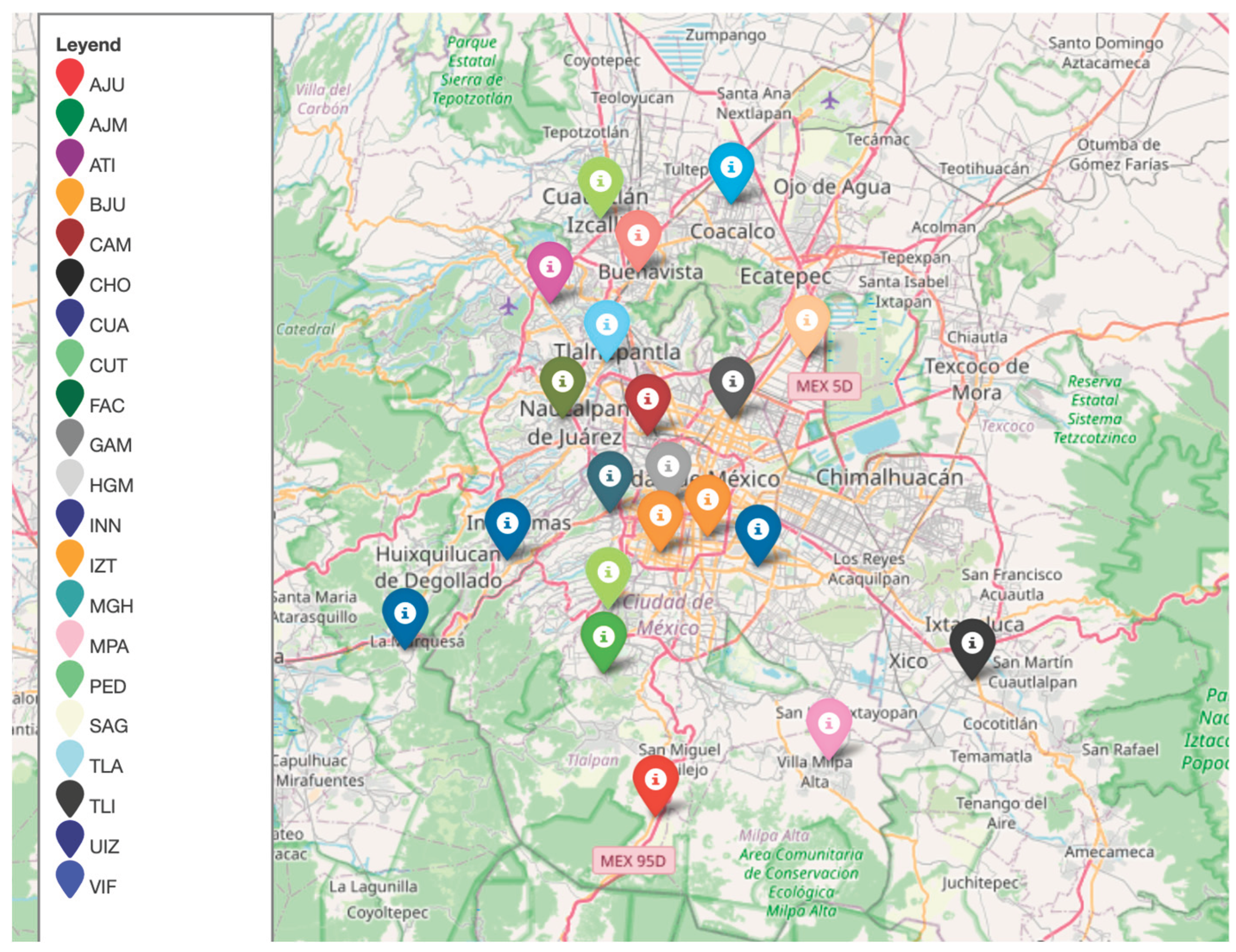
Figure 2.
Hourly variation of SO₂ concentrations at the UIZ monitoring station during 2024.
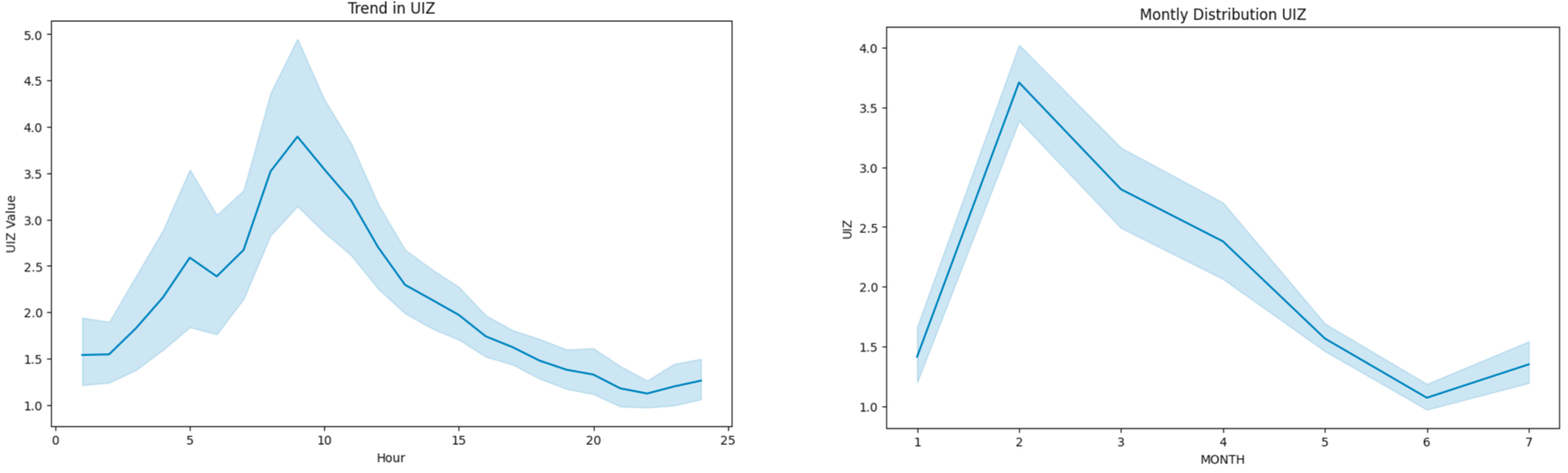
Figure 3.
Hourly mean ozone (O₃) concentrations in ppb (parts per billion) during 2024 at the UIZ monitoring station.
Figure 3.
Hourly mean ozone (O₃) concentrations in ppb (parts per billion) during 2024 at the UIZ monitoring station.
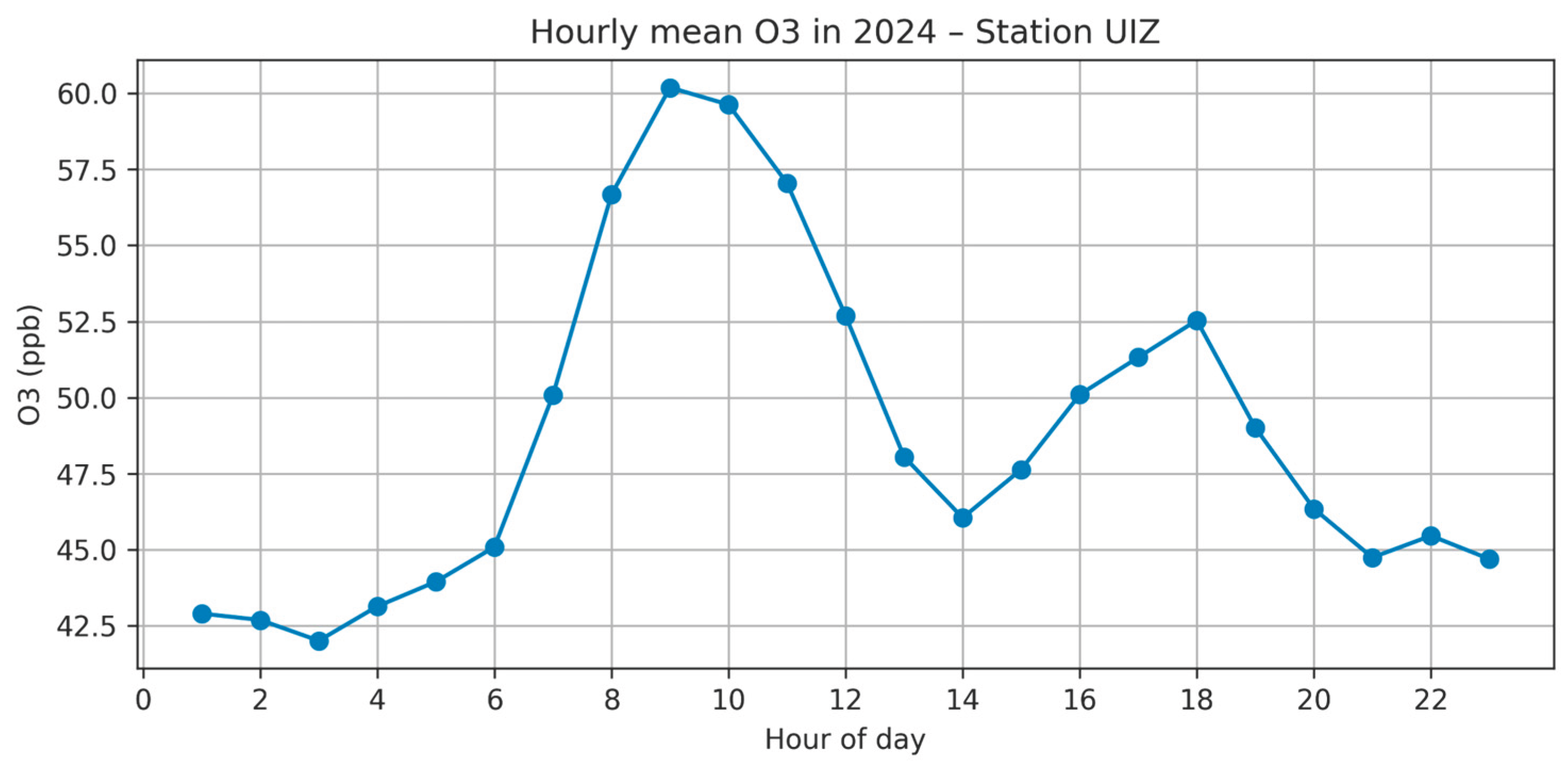
Figure 4.
Hourly mean SO₂ concentrations in 2024 at the CUA monitoring station.
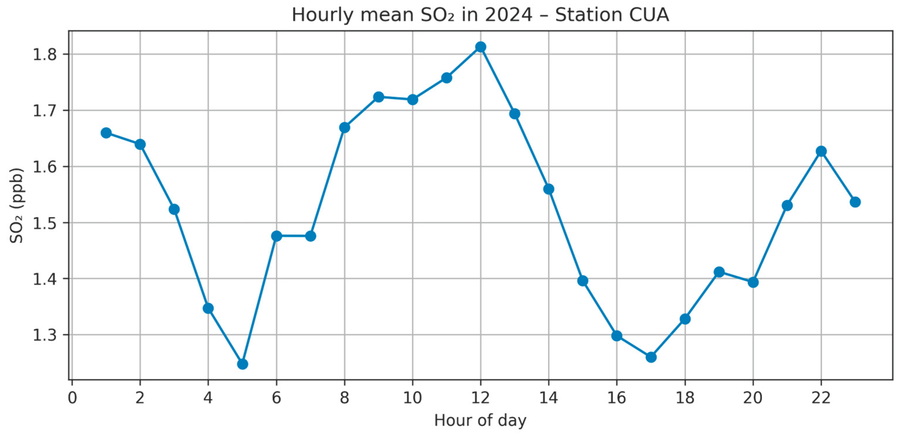
Figure 5.
a) Kriging interpolation map, b) Uncertainty map, O₃, Hour 15:00, Month May 5.
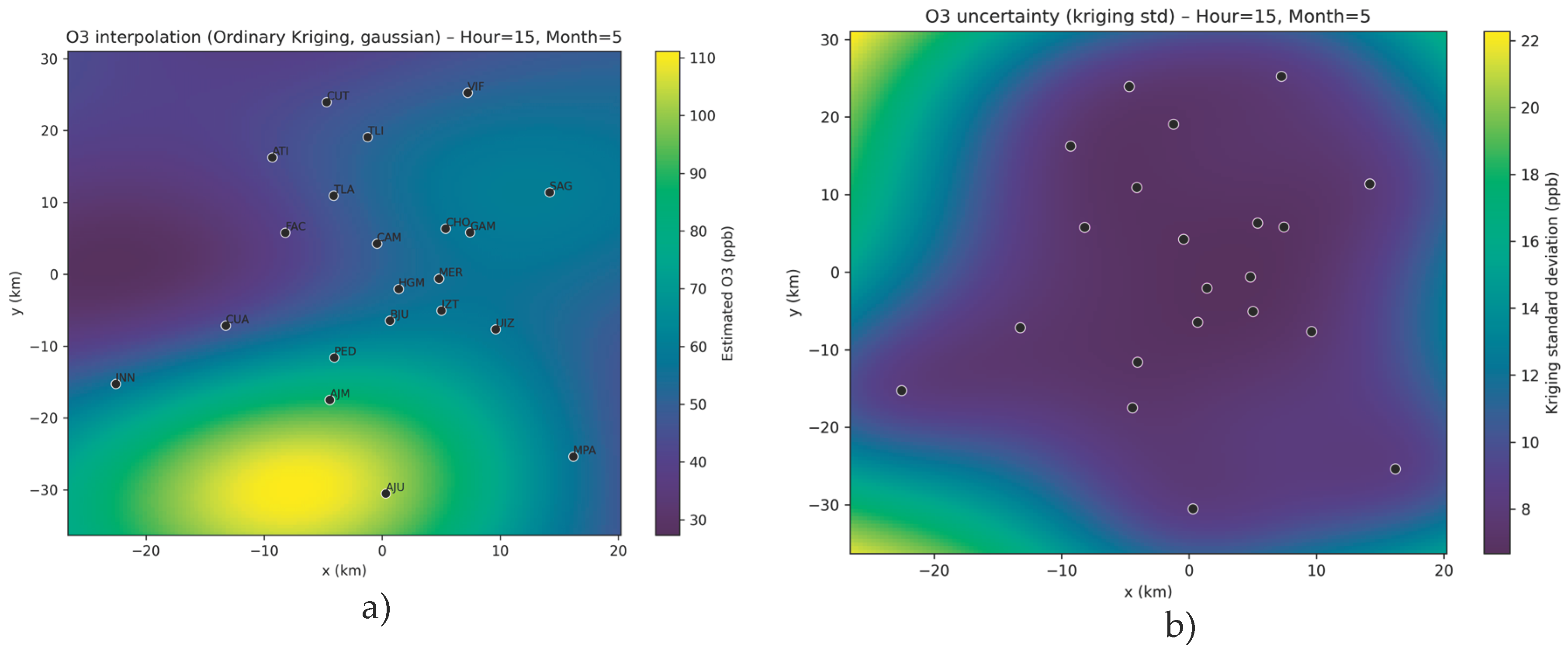
Figure 6.
a) Kriging interpolation map, b) Uncertainty map, SO2, Hour 10, Month 2.
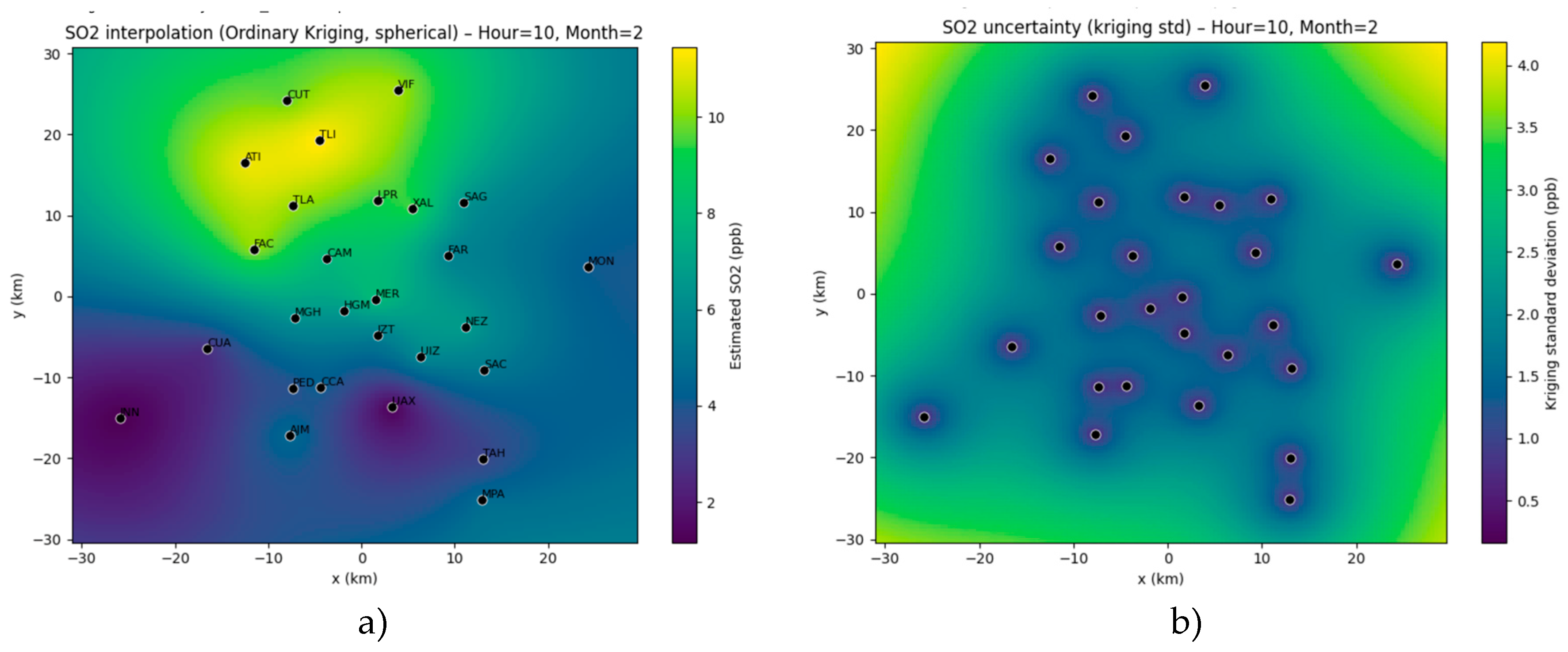
Figure 7.
Sensitivity of OK performance to temporal conditions. On the left, the sensitivity analysis shows that the smooth guassian model works the best, whereas on the right exponential and spherical models have a better fit.
Figure 7.
Sensitivity of OK performance to temporal conditions. On the left, the sensitivity analysis shows that the smooth guassian model works the best, whereas on the right exponential and spherical models have a better fit.
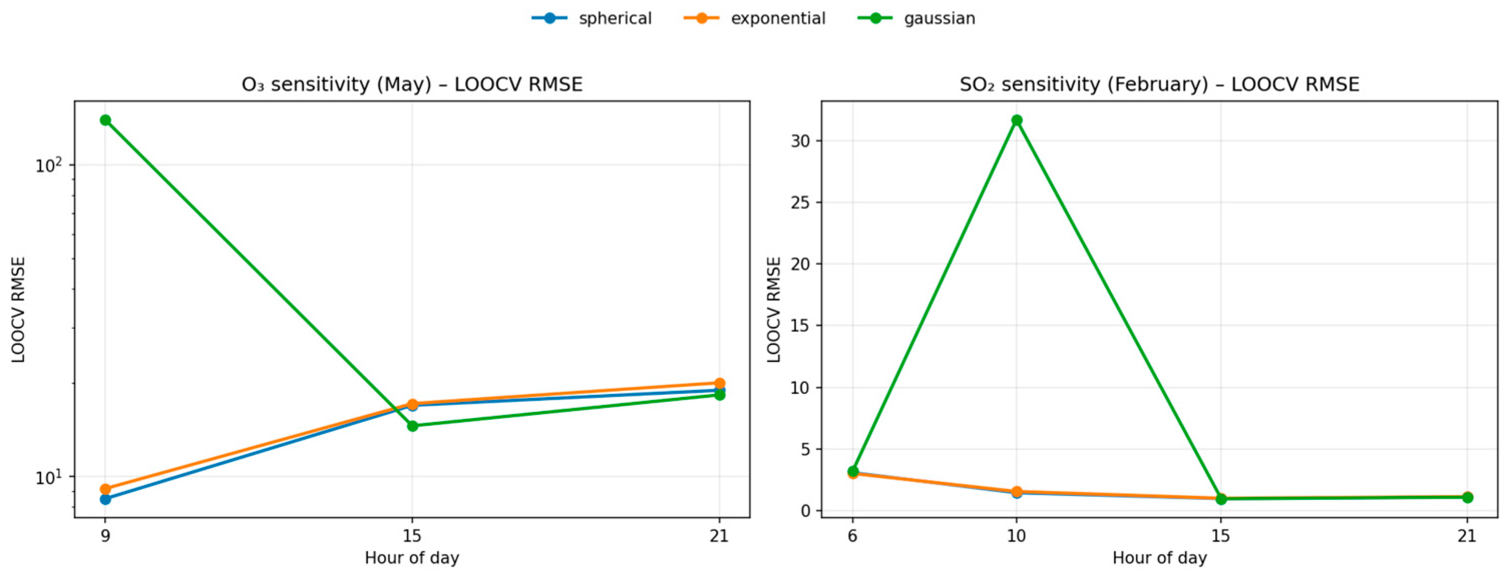
Table 1.
Monthly descriptive statistics at UIZ station, O₃, 2024.
| month | mean | median | std | min | max | n | p25 | p75 |
|---|---|---|---|---|---|---|---|---|
| 1 | 46.64188 | 42.52162 | 19.99761 | 10.51613 | 135.1667 | 460 | 33.59821 | 57.14259 |
| 2 | 51.96884 | 47 | 22.83287 | 16.24138 | 171.0769 | 483 | 37.20761 | 63.97222 |
| 3 | 55.55699 | 51.72727 | 20.98059 | 15.03226 | 166.3333 | 483 | 42.01613 | 64.73656 |
| 4 | 54.50459 | 52.92 | 17.30289 | 15.03704 | 112.1429 | 483 | 42.52013 | 63.89286 |
| 5 | 58.03709 | 55.03571 | 17.71254 | 19.53846 | 128.3333 | 483 | 46.73157 | 65.48746 |
| 6 | 37.87682 | 35 | 12.60866 | 14 | 90.2069 | 483 | 29.70417 | 42.94 |
| 7 | 30.3972 | 29.03704 | 9.253548 | 14.19048 | 70.78571 | 437 | 24.23077 | 35.86364 |
| 8 | 27.1636 | 24.90476 | 11.89331 | 8.157895 | 90.32258 | 435 | 19.425 | 33.69587 |
Table 2.
Descriptive statistics by hour at UIZ station during May, O₃, 2024.
| Hour | mean | median | Std | min | max | n | p25 | p75 |
|---|---|---|---|---|---|---|---|---|
| 1 | 38.2619 | 35.04348 | 16.57394 | 10.5 | 103 | 163 | 26.42955 | 46.21667 |
| 2 | 36.01109 | 33.375 | 15.10307 | 9.411765 | 88.5 | 163 | 24.875 | 44.82923 |
| 3 | 34.54254 | 33.28571 | 14.65417 | 9.176471 | 83.5 | 163 | 23.24815 | 42.76157 |
| 4 | 34.3171 | 32.22222 | 13.91843 | 8.157895 | 72.84615 | 163 | 22.80645 | 43.53784 |
| 5 | 34.39122 | 32.96 | 14.73063 | 8.730769 | 82 | 163 | 22.38889 | 43.86 |
| 6 | 37.21212 | 34.84 | 16.71861 | 9.423077 | 89.83871 | 163 | 24.79755 | 47.75714 |
| 7 | 43.56984 | 39.5 | 21.13661 | 8.962963 | 116 | 163 | 27.26154 | 55.69355 |
| 8 | 52.07109 | 45.55556 | 27.9995 | 10.38462 | 153.25 | 163 | 29.72989 | 68.98103 |
| 9 | 55.46481 | 48 | 28.98378 | 11.5 | 171.0769 | 163 | 33.85809 | 72.21667 |
| 10 | 54.58491 | 53.20833 | 24.2602 | 12.37037 | 135.1923 | 163 | 35.7577 | 68.81167 |
| 11 | 51.65196 | 51.83871 | 17.88423 | 13.40741 | 103.6 | 163 | 37.54839 | 62.25403 |
| 12 | 48.17588 | 47.44 | 14.11244 | 16.11538 | 96.93333 | 163 | 38.04849 | 57.81731 |
| 13 | 46.07734 | 45.43333 | 15.03253 | 19.5 | 110.3667 | 163 | 35.27381 | 51.98 |
| 14 | 46.85535 | 43.37931 | 17.8491 | 20.85714 | 116.1333 | 163 | 34.1523 | 53.17324 |
| 15 | 47.69461 | 45.98601 | 18.34663 | 14.25 | 114.0968 | 162 | 33.57955 | 56.18407 |
| 16 | 49.91696 | 48.20172 | 18.34619 | 21.3913 | 115.7895 | 162 | 36.09596 | 58.99107 |
| 17 | 52.03073 | 51.75 | 19.25995 | 17.64 | 111.2105 | 163 | 37.24702 | 60.63333 |
| 18 | 54.46105 | 52.55556 | 23.43304 | 17.11111 | 166.3333 | 163 | 37.03448 | 66.50862 |
| 19 | 53.42305 | 51.3 | 23.03444 | 16.33333 | 128.3333 | 163 | 38.18122 | 66.2963 |
| 20 | 49.52446 | 47.43478 | 20.56966 | 13.07407 | 109 | 163 | 35.39091 | 61.58796 |
| 21 | 46.4017 | 44.47368 | 19.08623 | 13.10714 | 105.9091 | 163 | 32.97222 | 55.16071 |
| 22 | 42.76662 | 40.72414 | 16.94158 | 13.82143 | 112.6 | 163 | 30.50278 | 50.79048 |
| 23 | 41.14418 | 39.30769 | 17.08175 | 12.36 | 120.2 | 163 | 29.43111 | 48.96552 |
Table 5.
LOOCVy Holdout Results, O3, Hour 15h, May.
| Model | LOOCV_RMSE | LOOCV_MAE | LOOCV_Bias | Holdout_RMSE | Holdout_MAE | Holdout_Bias |
|---|---|---|---|---|---|---|
| spherical | 16.9307 | 10.8707 | -0.1935 | 9.3855 | 7.8362 | -3.0027 |
| exponential | 17.1476 | 10.8138 | -0.2868 | 9.5189 | 7.9918 | -2.8750 |
| gaussian | 14.5492 | 8.81597 | -2.6317 | 10.3491 | 8.9841 | -3.1821 |
Table 6.
LOOCVy Holdout Results, SO2, Hour 10h, February.
| Model | LOOCV_RMSE | LOOCV_MAE | LOOCV_Sesgo | Holdout_RMSE | Holdout_MAE | Holdout_Sesgo |
|---|---|---|---|---|---|---|
| spherical | 1.451685 | 1.248203 | 0.102410 | 2.334734 | 2.175746 | 2.175746 |
| exponential | 1.552509 | 1.293633 | 0.123260 | 2.253626 | 1.956587 | 1.956587 |
| gaussian | 31.701103 | 11.507313 | -6.369781 | 9.378000 | 8.416435 | -0.454333 |
Table 7.
LOOCV cross validation; 9,15 and 21 hours, O3.
| Model | RMSE 9h | RMSE 15 h | RMSE 21 h | MAE 9h | MAE 15 h | MAE 21 h |
|---|---|---|---|---|---|---|
| spherical | 8.492602 | 16.9307 | 18.917307 | 6.429629 | 10.8707 | 15.973494 |
| exponential | 9.147813 | 17.1476 | 19.991709 | 6.685627 | 10.8138 | 17.044828 |
| gaussian | 139.533149 | 14.5492 | 18.285069 | 68.107795 | 8.81597 | 15.263694 |
Table 8.
LOOCV cross validation; February, May and August, O3.,.
| Model | RMSE February | RMSE April |
RMSE May |
RMSE August |
MAE February |
MAE April |
MAE May |
MAE August |
|---|---|---|---|---|---|---|---|---|
| spherical | 13.9780 | 17.3940 | 16.9307 | 16.094464 | 11.2406 | 11.8240 | 10.8707 | 9.906506 |
| exponential | 13.5090 | 17.4597 | 17.1476 | 16.391183 | 10.8734 | 12.3449 | 10.8138 | 10.640398 |
| gaussian | 14.4782 | 17.9417 | 14.5492 | 26.260674 | 11.2225 | 11.9900 | 8.8159 | 16.300298 |
Table 9.
LOOCV cross validation; 6,10, 15 and 21 hours, SO2.
| Model | RMSE 6 h |
RMSE 10 h |
RMSE 15 h |
RMSE 21 h |
MAE 6h |
MAE 10 h |
MAE 15 h |
MAE 21 h |
|---|---|---|---|---|---|---|---|---|
| spherical | 3.0721 | 1.4516 | 0.9739 | 1.1092 | 2.1219 | 1.2482 | 0.7323 | 0.9020 |
| exponential | 3.0080 | 1.5525 | 1.0012 | 1.1321 | 2.0817 | 1.2936 | 0.7616 | 0.9104 |
| gaussian | 3.1889 | 31.7011 | 0.9603 | 1.0880 | 2.4605 | 11.5073 | 0.7342 | 0.8950 |
Table 10.
LOOCV cross validation; February, April and August hours, SO2.
| Model | RMSE February | RMSE April |
RMSE August | MAE February | MAE April |
MAE August |
|---|---|---|---|---|---|---|
| spherical | 1.4516 | 1.524637 | 1.093720 | 1.2482 | 1.146517 | 0.792070 |
| exponential | 1.5525 | 1.556291 | 1.042159 | 1.2936 | 1.180675 | 0.756114 |
| gaussian | 31.7011 | 54.040358 | 41.609238 | 11.5073 | 25.105067 | 9.331594 |
Disclaimer/Publisher’s Note: The statements, opinions and data contained in all publications are solely those of the individual author(s) and contributor(s) and not of MDPI and/or the editor(s). MDPI and/or the editor(s) disclaim responsibility for any injury to people or property resulting from any ideas, methods, instructions or products referred to in the content. |
© 2026 by the authors. Licensee MDPI, Basel, Switzerland. This article is an open access article distributed under the terms and conditions of the Creative Commons Attribution (CC BY) license (http://creativecommons.org/licenses/by/4.0/).
Copyright: This open access article is published under a Creative Commons CC BY 4.0 license, which permit the free download, distribution, and reuse, provided that the author and preprint are cited in any reuse.


