Submitted:
07 February 2026
Posted:
09 February 2026
You are already at the latest version
Abstract
The smart agriculture system requires high efficiency to automatically maximize crop yields and minimize losses. Wireless sensor networks (WSNs) are essential for maintaining system sustainability through sensing and connectivity. However, they encounter challenges related to cost, interoperability, and reliability. Efforts have been made to expand sensing capabilities while managing costs and addressing variability in sensor communication and power consumption. Despite these efforts, a comprehensive solution—especially for orchard fields—remains undeveloped. This study introduces a coordinated WSN design to optimize sensing and connectivity in agricultural fields. We employ an integrated sensing and connectivity (ISAC) strategy to create a complete solution. Our hybrid approach combines graphical computation with distance-vector algorithms for reliable, cost-effective deployment. Additionally, resilient connectivity is achieved through effective channel modeling and adaptive beamforming. The proposed method, combined with quantitative heterogeneous network selection using MLR-AHP, addresses interoperability issues and improves network resilience. Results indicate improved sensor placement and wireless ranking, even with only 5 nodes. The solution extends sensor battery life, maintains 99% coverage, and empirical tests validate its effectiveness for designing and deploying WSNs in orchard fields.
Keywords:
smart agriculture system
; WSN
; sustainability
; heterogeneous wireless
; MLR-AHP
; RDT
; coverage
; lifetime
; optimization
; area sampling
1. Introduction
The global population growth is causing a significant food shortage, affecting about 40% of the world's population [1]. Key factors include inadequate food storage and low production rates. Initiatives to incorporate e-commerce and digital technologies into storage and logistics are ongoing [2]. While these methods are beneficial, they still lag behind the rising food demand. Increasing agricultural productivity and minimizing losses are generally considered more effective strategies [3]. However, challenges such as shrinking farmland, labor shortages, declining water supplies, and climate change hinder productivity growth. Researchers are keenly exploring new agricultural techniques to tackle these issues. Among them, smart agricultural systems hold great potential to boost output, reduce labor requirements, and reduce waste [4]. These systems utilize IoT technology, which provides advanced features and relies mainly on three key processes: data collection, analysis, and management [5]. These processes are essential to agricultural advances in Industry 4.0, as illustrated in Figure 1.
The data acquisition phase involves collecting soil, water, climate, and plant trait data using stationary, mobile, or satellite-based sensors. Fixed sensors are most common due to their reliable performance. These sensors transmit data to the control unit for analysis and decision-making, and to the central system for further processing. Maintaining sustainable sensing and reliable connectivity is essential, as poor connections can disrupt data flow and threaten system sustainability [6]. The wireless sensor network (WSN) provides the primary infrastructure for data collection and exchange, requiring an efficient, distributed farm network.
Allocating fixed sensor nodes is crucial yet challenging due to uncertainty. The main challenge is how to distribute these nodes efficiently to cover the area with the fewest sensors. There is a trade-off between minimizing the number of sensors and ensuring effective data collection [7]. Field sensing is essential for the operation and management of smart agriculture systems. Reducing the number of sensing elements may lead to insufficient data, resulting in incorrect decisions and potential losses. Over the last decade, sensor technology has advanced significantly, offering greater capabilities but at higher per-node costs. The latest development is integrated sensing and communication (ISAC), which turns sensing units into fully capable nodes that can sense, process, and communicate [8]. This innovation has led many manufacturers and developers to produce such nodes. However, the lack of standards across manufacturers has caused interoperability issues, complicating sensor node deployment [9].
Field sensing uses various sensors to measure infrequently changing physical parameters, thereby reducing the need for widespread deployment. Weather parameters vary over large regions, so extensive sensor coverage isn’t necessary. However, modern systems recommend a balanced distribution of sensors across different functions. Temperature sensors can detect anomalies, such as fires, early. Humidity sensors monitor issues like water stress or infections [10]. Soil parameters such as temperature, humidity, pH, and salinity are assessed using targeted samples. Soil sensors should be evenly spaced to detect heat stress, root infections, flooding, or leaks. Salinity sensors are useful in dense weed areas [11]. Proprietary sensing offers benefits but doesn’t eliminate the need for broad coverage. Reliable autonomous systems depend on continuous monitoring; inaccurate data can impair decisions, underscoring the importance of proper sensor placement. The shift toward regenerative agriculture and climate adaptation emphasizes dense field sensing [12]. This dense sensing, in turn, requires improved connectivity, especially in orchard fields [13].
Enhanced wireless coverage for sensor nodes reduces power consumption and prolongs device lifespan [14]. Improved coverage decreases the power needed for reliable communication. Wireless connectivity is vital for sustainable smart agriculture, supporting both in-field and backhaul links. Although both are crucial, the growth of edge processing shifts attention toward in-field connectivity. Factors such as terrain, foliage, and obstacles, as well as poor coverage, affect sensing and connectivity, with foliage and leaves posing major obstacles [15]. Network interoperability issues and dead zones disrupt connectivity and data flow. An unreliable backhaul risks system management and cloud-edge architecture. Power and energy constraints threaten sustainability, especially for rapid response, high-bandwidth agricultural monitoring [16]. These challenges must be considered during the design process. The type of agricultural field influences design, as land and plant parameters can weaken signals, especially in orchards with dense foliage and tall trees. Beyond their economic value, orchards are particularly significant.
Numerous studies aim to improve wireless communication, sensor placement, and system reliability [17]. The diverse range of wireless options in WSN equipment also presents challenges [18]. At the same time, cost-effective sensor deployment in agriculture is highly sought after [19]. While creating efficient WSNs guarantees reliable sensing and connectivity, this remains an active research area. To our knowledge, no existing work combines sensor deployment and wireless coverage into a single solution. This paper introduces a novel WSN design that enhances sensing coverage and wireless connectivity [20]. Its primary goal is to enable dependable, real-time data collection with minimal cost and power consumption. A secondary aim is to support heterogeneous wireless communication to address interoperability issues. Additionally, the paper aims to improve capacity planning and data management through a comprehensive fixed-sensing strategy. The structure includes sections on related work, methods, simulations, analysis, results, discussion, and conclusions.
The proposed method employs optimized sensor placement, signal modeling, and decision-making processes to select the most suitable wireless technology. The main contributions are summarized below:
- This study proposes a hybrid method combining geometric principles and random sampling to identify optimal field zones. It ensures thorough coverage, efficient processing, and balances accuracy with adaptability, improving environmental data collection.
- The wireless node distribution model employs a distance-vector algorithm combined with signal-range constraints to optimize sensor placement within the sampling area. It addresses orchard-specific wireless issues, such as signal attenuation and interference, to ensure reliable communication, reduce coverage overlap, and save energy.
- A hybrid regression–Analytic Hierarchy Process (MLR-AHP) model ranks wireless communication technologies by combining regression analysis with the AHP comparison matrix. This provides an objective ranking that supports informed decisions, considering agricultural conditions, range, and power limitations.
- Progress in precision agriculture and smart farming is propelled by ISAC-based WSN design, which improves data gathering, connectivity, and sustainability. This facilitates real-time monitoring, better decision-making, and more efficient resource utilization, leading to increased sustainable productivity.
2. Related Work
The design of WSNs in smart agricultural systems is characterized by considerable uncertainty. Since ISAC is the primary driver of the design, it is more effective to treat coverage as a key sensing goal. The primary challenge is to balance reducing deployment expenses while ensuring reliable field-parameter sensing.
Extensive research has explored how to locate sensor nodes in agricultural regions. Satellite remote sensing provides a potentially affordable backhaul option, as mentioned in [21]. Yet, this approach faces limitations in accuracy and visibility caused by cloud cover and tends to become more costly over time. Drones, as discussed in [22], present an economical alternative to satellite systems. Nevertheless, satellite imagery generally offers greater potential than drone-based analysis. Despite this, using drones to monitor plant health is extremely useful for evaluating growth rates and nutritional status [23] and for predicting yields [24]. Still, significant challenges persist, including complex path planning, reliable communication, and effective charging management.
On the other hand, stationary sensing enhances the analysis of soil characteristics, provides more accurate weather monitoring, and facilitates improved water sensing, as outlined in [25]. There are three primary approaches to addressing uncertainty in sensor node allocation: probabilistic, stochastic, and deterministic [26]. Probabilistic allocation involves distributing sensor nodes based on their relevance to agricultural objects. In contrast, stochastic methods enable better allocation with fewer sensors and a broader sensing range, thereby reducing overlap, as shown in [27]. Deterministic allocation yields the optimal sensor placement relative to the sensing target, as described in [28]. Better solutions can be achieved by adding clustering techniques, as noted in [29]. In addition, the most effective optimization arises from a systematic distribution tailored to the specific area, as mentioned in [30]. Deterministic distributions include various systematic arrangements, such as the systematic grid [31], the hexagonal pattern [32], and the triangular layout [33]. Several methods are employed to optimize sensor allocation, including particle swarm optimization (PSO) [34], annealing [35], and the Gaussian distribution of sensor nodes [36].
Additionally, alternative methods such as mathematical sensor allocation [37], graphical computation-based allocation [38], and a hybrid approach have been explored. Many hypotheses regarding sensing range and wireless coverage lack robust support, particularly regarding coverage within the area of interest. That still doesn’t align with the ISAC approach in the agricultural field.
An often-overlooked aspect of sensor deployment is providing simultaneous, relevant wireless coverage, which also encompasses sensor connectivity diversity. Most research emphasizes sensor placement rather than wireless technologies. Satellite technology offers a backhaul solution for cloud WSNs, as shown in [39], but it is costly to implement, making satellite-capable sensors rarely used. Nb-IoT is viewed as a more affordable option for cloud-edge systems, yet its effectiveness depends on service availability, as in [40]. LoRaWAN provides a more economical alternative compared to satellite and NB-IoT; however, its low bit rate and bandwidth restrict its use to low-data-rate sensing, excluding photo or video applications, as in [41]. Bluetooth presents a promising low-cost, low-rate deployment option for clustering, as in [42]. Wi-Fi offers high data rates and low deployment costs, making it suitable for clustering, as in [43].
Several practical studies have explored WSN design by identifying the optimal clustering strategy with respect to the top approach, which offers a more scalable solution, as discussed in [44]. It also helps reduce complexity and traffic latency, particularly in full-mesh WSNs, as shown in [45]. Additionally, it enhances processing and management at the edge devices, as indicated in [46]. However, the study in [47] identified the optimal clustering strategy with respect to deployment costs. Considering the impact of planting on the WSN, especially on infield connectivity among sensor nodes, is also very desirable. A practical study of deploying a WSN with adaptive beamforming to maintain connectivity is presented in [48]. Figure 2 summarizes the WSN design approaches.
This paper investigates graphical computation for clustering the entire area into samples through deterministic and probabilistic allocation. Furthermore, it aims to present a mathematical solution within a square deterministic grid framework. The study will empirically examine Voronoi clustering as an effective method for assessing sensing and connectivity. The goal is to develop an algorithm that improves sensing range, cuts costs, extends lifespan, and boosts connectivity.
3. Methodology
The methodology of the proposed hybrid solution is split into two main sections.
- Wireless coverage to address the sensors’ interoperability issues.
- Fixed sensor localization, which reduces the uncertainty of the sensor distribution.
The research methodology makes the following assumptions for conducting the study:
- 1)
- The orchard field is flat and stable, facilitating strategic placement of sensors in two dimensions. Nonetheless, the study also examines how vegetation impacts wireless communication in three dimensions. The research study incorporated adaptive beamforming for the orchard field wireless channel.
- 2)
- Sensor nodes are categorized into two types: Type 1 and Type 2. Type 1 nodes, fully equipped with sensors, act as the central anchor, while Type 2 nodes, partially equipped, surround it.
- 3)
- Besides built-in sensors, sensing nodes connect to external sensing elements. Wireless communication metrics are numerous. The study used a quantitative approach to select a pair of heterogeneous wireless networks.
- 4)
- The research employed a mixed-methods approach across three stages: initially, clustering the area using graphical computation; second, deploying sensor nodes through a grid, distance vector, and mathematical methods; and third, validating sensor nodes with Voronoi tessellation, adaptive beamforming, and RSSI enhancement.
The methodology enhances wireless coverage and sensor placement by fixing power and connectivity issues for reliable links. It employs various wireless technologies for broad coverage and minimal power use by connecting only to relevant nodes. A quantitative approach ranks wireless sensor options. Sensor localization uses a hybrid algorithm with graphical computation and distance vectors, as shown in Figure 3.
The methodology streamlines sensor deployment by employing clustering to pinpoint areas of interest, optimize placement, and minimize the number of sensor nodes. It accounts for wireless constraints and distance vector routing, ensuring high-density coverage and reliable connectivity. Furthermore, it evaluates and ranks appropriate wireless technologies for integration, reducing delay and power consumption.
4. Methods
4.1. An Algorithm for Ranking Wireless Technologies:
This section covers solutions for dependable wireless connectivity in industrial sensors. The algorithm shown in Figure 3 creates a heterogeneous wireless infrastructure. Achieving system reliability requires leveraging multiple wireless technologies to meet the connectivity demands of the agricultural system, illustrated in Figure 1. While interest in heterogeneous networks is increasing, decision-making methods based on multiple criteria (MCDM) remain common [49]. The most widely used MCDM method is the Analytical Hierarchy Process (AHP) by Saaty [50], valued for its straightforwardness and for its ability to structure complex decisions into a hierarchy, as explained below.
goals → criteria → sub-criteria → alternatives.
This clarity aids in solving multidisciplinary problems by evaluating technologies based on bandwidth, lifetime, delay, and plant health. The Pairwise Comparison Matrix assesses two items at a time, such as "Is coverage more important than bandwidth?" Properly constructing the matrix reduces cognitive load, particularly for experts who may find quantitative methods difficult. Accuracy in this process is essential.
The Analytic Hierarchy Process (AHP) translates qualitative judgments into quantitative weights by integrating technical data and expert opinions. It employs a consistency ratio (CR) to ensure judgment reliability. The pairwise comparison matrix impacts ranking results and varies, highlighting differences between qualitative and quantitative evaluations. Generating multiple matrices from a qualitative scale can lead to inconsistencies. To mitigate this, approaches like Fuzzy-AHP (FAHP) have been introduced. While matrix construction refines weights, FAHP's advanced techniques do not fully address the underlying problem. A hybrid method leverages machine learning, particularly multiple linear regression (MLR), which is simpler and more transparent than fuzzy methods. MLR models the relationships among wireless network options, attributes, and goals through an equation that computes a usability score based on delay (D), bandwidth (B), power (P), range (R), environmental impact (H), and capacity (C), as:
where:
Y= β0 + β1D + β2B + β3P + β4R + β5H + β6C + ε
- β₀ represents the baseline value, unaffected by the parameters.
- ε is an error term used to adjust the equation's sides.
- Y denotes the Usability Score
- βi corresponds to the coefficients, with i ranging from one to six.
Equation 1 describes traffic across wireless technologies such as Wi-Fi, Bluetooth, Zigbee, LoRa, NB-IoT, and 5G [51], which serve as the basis for the comparison matrix. During a two-week period, six sensing nodes communicated with a controller, while a Python-based simulator generated a synthetic dataset that mimicked realistic behavior [52]. The total traffic for each node was calculated as a weighted sum with added noise to account for environmental variability. Data were then aggregated by protocol for AHP analysis, and the regression coefficients are presented in Table 1.
The pairwise comparison matrix employs the average total traffic scores for each protocol. Each element aij indicates the significance of protocol i relative to j, as described as:
aij = scorei/scorej
The matrix is reciprocal, indicating that for each element aij, the corresponding element aji is its reciprocal, 1/aij. This matrix is used as input in the AHP ranking process.
Figure 4.
Process flowchart for heterogeneous wireless network coverage.
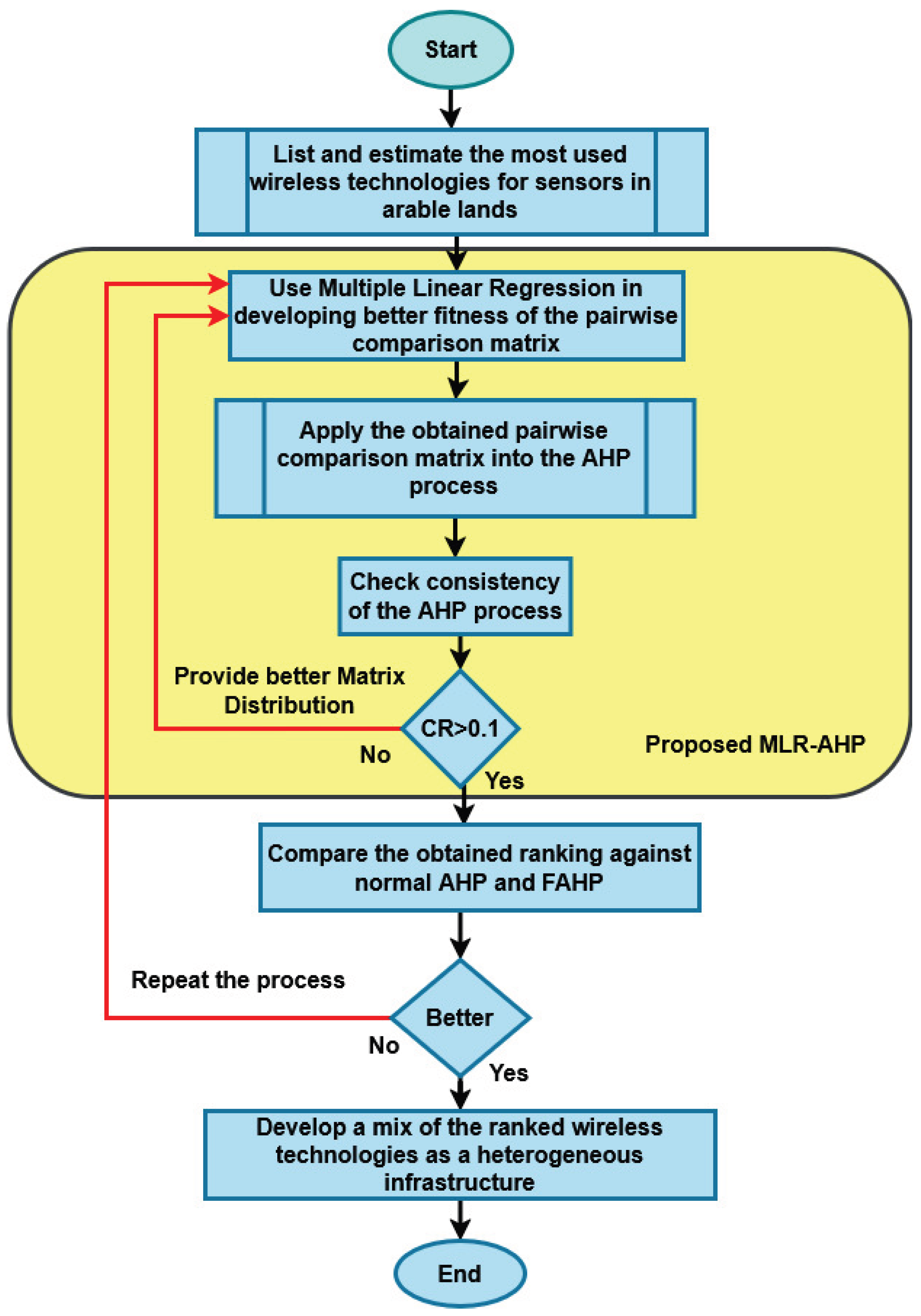
The methodology employs the AHP to establish a weight vector that ranks wireless networks. The AHP process comprises these steps:
Create a composite score for each technology using MLR following equation (1). Then, compute the scores for each technology based on normalized inputs. Calculated the normalized weights for each protocol as follows:
- Column normalization: Divide each element by the total sum of its column.
- Row averaging: The mean of each row in the normalized matrix defines the weight of the protocol.
These weights indicate the relative significance of each protocol based on the combined metrics.
- 1.
- Apply AHP: AHP simplifies complex decisions into pairwise comparisons, synthesizing results to derive weights and rankings based on specific criteria:
- •
- Coverage: Influenced by Range & Capacity
- •
- Lifetime: Influenced by Power Consumption
- •
- Plant Health Impact: Influenced by Delay & Impact score
- •
- Bandwidth: Directly influenced by Bandwidth
The dataset included 6 nodes over 14 days, yielding 504 measurements (6 protocols × 6 nodes × 14 days) [52]. This sample size was enough to reduce variability in protocol scoring and maintain consistency in the AHP pairwise comparisons. The goodness of fit was implicitly confirmed through:
- Consistency Ratio (CR): Ensures reliability of pairwise judgments.
The Consistency Ratio (CR), computed using equation 3, is used to verify the logical consistency of the pairwise comparisons.
where:
CR= CI/RI
- CI is the consistency index, calculated through:
CI = [(λmax–n)/(n-1)]
- λmax is the maximum eigenvalue of the pairwise matrix
- n is the number of protocols
- is the Random Index for alternative
- The RI value in the AHP process is 1.24 for six alternatives.
The pairwise comparison matrix is consistent if CR ≤ 0.1. It maps attributes to criteria and develops priority matrices. Table 2 shows the wireless ranking results based on coverage distance.
The coverage distance extends the wireless network, ensuring sensor connectivity. Wireless coverage is vital to system sustainability, as it relies on a stable wireless infrastructure. Sensors are hardware-constrained, and their lifetime affects system trustworthiness. Wireless networks are ranked by power consumption, as shown in Table 3.
Power consumption is key when choosing wireless networks. Less power-hungry connections are better, extending sensor life and supporting sustainability. Wireless signals also impact plant health, especially growth rates. Longer connection times have greater effects, as shown in Table 4.
Delay rates evaluate wireless connectivity quality by ranking connections from least to most impact, as described in [53]. Data-acquisition nodes typically need high data rates, particularly for plant images. Bandwidth, an essential metric, orders networks from highest to lowest, as shown in Table 5.
Wireless connection bitrates show that higher speeds generally provide more reliable plant image transmission. Once these four rankings are determined, the AHP process uses them to identify the most appropriate wireless connection ranking. This helps determine the optimal data offloading strategy in a dense, mixed wireless network.
4.2. Deploying Sensors in a Way That Minimizes Costs While Maximizing Sensing Coverage
The approach uses a deterministic sensor placement strategy. It positions the anchor node (Type 1) at the field's center, with other sensor nodes (Type 2) surrounding it. The Type 1 node has all sensing components for normal and abnormal detection, while the Type 2 node has only the essential sensing elements. Both node types share the same shape, as shown in Figure 5.
The Figure illustrates a sensing node that includes a tripod, an antenna, a weather station, a soil sensor, and a junction box. The tripod provides ground support and stability for the sensor system. The antenna, mounted at the top of the tripod, transmits wireless signals by converting electromagnetic waves into electrical signals and connecting to the gateway via a cable in the junction box. Above the antenna, the weather station contains sensors to measure various weather parameters. The soil sensor, installed in an underground tube, monitors soil conditions and is connected to the gateway via a cable in the junction box. The junction box attached to the tripod safeguards the components and houses the power supply, photovoltaic unit, controller, gateway, UV-index sensor, ultrasonic sensor, infrared sensor, and camera.
The anchor node (Type 1) is a fully equipped sensor node that includes:
- A high-capability embedded system board enabling communication and data analysis for sensor nodes, installed within the junction box.
- The weather station sensors measure temperature, humidity, dew point, UV index, rainfall, and wind. This unit connects to the controller with a cable and communicates wirelessly with the junction box.
- Soil-sensing sensors measure temperature, humidity, pH, and salinity. The sensing element is housed inside a tube extending into the soil. This unit connects to the controller via cable and wireless links through the junction box.
- Sensors for plant health, such as distance, motion detection, and infrared, are installed inside the junction box.
- The photovoltaic unit supplies energy to the controller, while the charging unit, with various components, is installed inside the junction box and the PV unit on its back cover.
Other sensor nodes are classified as minimally equipped (Type 2), able to detect and measure various agricultural physical parameters such as:
- A compact system board connects sensors and communicates with a controller.
- Weather sensors detect temperature, humidity, smoke, and UV index, connected via cable and wirelessly through the junction box.
- Soil sensors for temperature and humidity are mounted in a tube in the soil, linking to the controller both wired and wirelessly.
- Plant health sensors measuring height, distance, motion, and infrared are installed inside the junction box.
- Power is supplied by the photovoltaic (PV) unit and power consumption components inside the junction box, with the PV unit on the junction's back cover.
The methodology involved enhanced assessment of weather, soil conditions, plant health, growth rates, and pest detection. Table 6 lists the sensor types used in the study, along with their connection types.
Wired sensors are mounted on the sensor node board, while wireless sensors offer more mounting flexibility within the grid. All sensors can measure physical parameters in various conditions. These considerations optimize placement and improve autonomous field monitoring. The study presents a method to allocate sensor nodes to maximize coverage with fewer nodes.
The flowchart in Figure 6 shows the WSN allocation algorithm. It begins with defining sensors' normal distribution over a square area, A(x, y), with x = y, as in Figure 5.
The agricultural zone is an orchard with trees, represented by T(x, y) and illustrated by green dots in Figure 7. The system's coverage, C(x, y), is the minimum number of sensor nodes needed to monitor area A(x, y) while optimizing sensing of T(x, y). The area size impacts sensor requirements and connectivity constraints. For Wi-Fi, the max range is about 150 meters, as in Figure 8 [61].
Best practice [62] recommends limiting Wi-Fi repeaters to three devices with at least 30% coverage overlap. Figure 8 shows three devices at distances greater than 150 m, and Figure 9 depicts a 300 m area around an anchor node. Uniform sensor distribution in this area results in excess sensors, so a distance-vector algorithm optimizes placement via graph analysis [63], maintaining device positions and neighbor relations [64], and clarifying communication dependencies through graph theory [65]. While aiding placement, it affects capacity and causes delays. To minimize sampling distance, the area is analyzed for optimal placement, often within mobile sensing solutions to reduce travel. Techniques like RRT are used for area sampling [66,67], though they may pick suboptimal sites. The proposed approach uses random exploration from fixed points, introducing a deterministic Rapidly Exploring Deterministic Tree (RDT), which selects multiple points to ensure effective, uniform sampling, as shown in Figure 9.
The proposed RDT algorithm is assessed by examining the distribution of blue and yellow points across the specified area, as illustrated in Figure 9. Blue points represent the primary probability distribution, while yellow points highlight deviations from this distribution by sensor nodes. These points assist in guiding the potential placement of sensor nodes within agricultural area A (x, y). The main area is divided into 36 sub-squares, each measuring 50 meters on a side. Blue points are scattered within these sub-squares with a 5-meter offset along the edges, and a yellow point is positioned 5 meters from the center, avoiding overlap and ignoring the edges and the bottom border. The RDT then uses these nodes to generate a closed-loop path, helping to identify areas of interest. The approach checks whether the new area of interest is smaller than 0.8 times the size of the central regions. Additionally, sensor nodes are allocated based on distance vectors to mitigate wireless limitations [57]. The system assumes a sensing range of 40 meters, as shown in Figure 10, with a maximum range of 50 meters.
The sensor node's wireless coverage radius, R2, is 50 meters, and its sensing range, R1, is 40 meters. These constraints guide proper node placement within the area. The algorithm maintains overlaps within the sensing range to improve communication and reduce redundancy. It iterates until stable communication and neighbor relationships are achieved. The performance is then compared to previous methods.
4.3. Wireless Communication Within the Orchard Field
Deploying a WSN in an orchard is more challenging than in an open field due to the "vegetative barrier" formed by trees. Ensuring reliable connectivity and precise data collection requires examining the field's physical and environmental conditions. This study details an orchard investigation, including analysis of orchard features, modeling of the wireless channel, and validation through Voronoi diagrams.
4.3.1. Orchard Field Characteristics
The placement of trees influences network topology, such as star, mesh, or cluster-tree configurations. Tree spacing and alignment are typically set in predictable rows, as shown in Figure 11. Sensor nodes placement is maintained efficiently through these rows to preserve a clear Line-of-Sight (LoS).
- Tree height determines antenna placement, ideally just above the canopy (2.5–3.0m) for maximum range, enabling signals to diffract over trees.
- Vegetation density affects signal attenuation; dense canopies, like mature citrus or mango orchards, need higher node density than sparser, younger apple trees.
4.3.2. Wireless Channel Modeling
The orchard's impact on wireless signals involves mechanisms like attenuation, scattering, shadowing, and seasonal changes [69]. Water in leaves absorbs RF energy, especially at 2.4 GHz. Small leaves scatter signals, trunks cause diffraction and multipath interference, creating fading. Large trunks form shadow zones with lost connectivity behind them. Seasonal changes affect signal quality, with wetter summer foliage reducing performance compared to winter. The model uses equations from a channel model, including Weissberger's Model, which estimates additional attenuation caused by dense vegetation beyond a 14 m threshold, approximated as:
Where:
- d = path length (m) through foliage
- The coefficient 0.45 dB/m is a typical attenuation slope for moderate vegetation at 2.4 GHz.
- COST 235 provides empirical estimates of attenuation for various foliage densities and frequencies. The model's general form relates attenuation to frequency and leaf depth. Equation 6 provides an empirical approximation at 2.4 GHz.
PLCOST235 (d) = 0.2 x (f 0.3) x (L 0.6) x (d/100).
Where:
- f = frequency in MHz
- L = one-sided foliage depth in meters
- d = path distance in meters
When integrated, each link's instantaneous (SNR) is expressed as:
SNR(d) = Pt − PLmodel(d) − N0.
Where: Pt is the transmitted power (dBm) and N0 is the noise floor (dBm).
4.3.3. RSSI Adaptive Beamforming Combined with Voronoi-Based Validation
To tackle these features, the following technical strategies are necessary:
- •
- Optimal node placement:
- ▪
- Near ground: Ideal for soil monitoring, but experiences high signal loss caused by the Fresnel zone obstruction from ground and weeds.
- ▪
- Mid-canopy: Subjected to significant attenuation due to dense foliage.
- ▪
- Above-canopy: Provides the longest range (up to 2-3 times farther than mid-canopy) but is more challenging to install and maintain.
- •
- Link quality metrics: Utilize RSSI (Received Signal Strength Indicator) to detect "blind spots" during the initial field survey. Combine this with Voronoi diagrams to create a realistic coverage pattern for each sensor node, accounting for the 3D effects of plants.
The adaptive beamforming is maintained through two steps [70]:
- (1)
- estimation technique for Direction of Arrival (DoA) estimation.
Consider M = eight antenna elements (at the controller) and K narrowband far-field signals (from sensor nodes); then, the array output vector can be modeled as:
x(t)=a(θ) x s(t) + n(t)
Where:
- x(t)∈CM×1 = received signal vector
- s(t)∈CK×1 = source signals
- Noise vector (AWGN) = n(t)∈CM×1
- a(θk) = steering vector for the kth source, K is a counter 1:8.
For a ULA with inter-element spacing d and wavelength λ the steering vector is expressed as:
Covariance Matrix Estimation: This method calculates the spatial covariance matrix using N snapshots, as:
Then perform eigen-decomposition, as:
Rx=EsAsEsH + EnAnEnH
Where:
- Es = signal subspace eigenvectors (largest K eigenvalues)
- En = noise subspace eigenvectors (smallest M−K eigenvalues)
Finally, MUSIC exploits the orthogonality between the steering vectors of the true sources and the noise subspace, which is expressed as:
PMUSIC (𝛉) = 1/ (aH (𝛉) En EnH a(𝛉))
The peaks of PMUSIC(θ) correspond to estimated DoAs. For M sensor nodes, MUSIC scans θ over [-90°, 90°] and detects M peaks.
- (2)
- Adaptive beamforming employs the least mean square (LMS) algorithm to optimize antenna weights, enhancing signal power in the DoA direction while reducing the error between the desired and received signals. The LMS algorithm is an iterative process that minimizes the mean squared error (MSE) between the beamformer's output and the reference signal. In the proposed approach, once MUSIC detects the DoAs of the eight sensor nodes, LMS adjusts the antenna weight vector to direct the main lobes of the radiation pattern toward those angles. This adjustment improves the reception of desired signals while minimizing interference. For an M-element ULA receiving the vector x(n) ∈ CM×1, the beamformer output is given as:
y(n)=wH(n)x(n)
Where: w(n)=[w1(n),w2(n),...,wM(n)]T represents the weight vector at time n. The goal of the adaptive beamforming method is to determine the optimal w(n) values that maximize RSSI.
- (3)
- Using Voronoi diagrams allows us to transition from qualitative field observations to quantitative verification of signal reliability (RSSI) [71].
Consider a set of sensor nodes S = {s1, s2, …., sn} deployed in an orchard, where each node Si is at a coordinate Pi that belongs to R2. A Voronoi Cell V(Si) is the set of all points q in the orchard that are closer to Si than to any other node Sj:
V(Si) = {q belongs to R2 ||q - pi|| less or equal ||q - pj||, for all j not equal i}
Where:
- ||q - pi|| is the Euclidean distance between a point and the sensor.
- The boundary between two cells V(si) and V(sj) is the perpendicular bisector of the line segment connecting si and sj.
To verify that RSSI is maintained despite foliage, we model the signal power Pr at any point q within the cell V(si) using the Log-Distance Path Loss Model:
Pr(q) = Ptx - L0 - 10n log10 ((||q - pi||)/d0) – PLmodel (d)
Where:
- n is the path loss exponent (n approx. 3 in dense orchards).
The Verification Condition
For the network to be considered "covered" and "connected," the RSSI at the farthest point of the Voronoi cell (the Voronoi vertices vmax) must exceed the receiver sensitivity threshold Pthreshold:
Ptx - L0 - 10n log10 ( ||vmax - p_i||/d0 ) – PLmodel (d) is greater than or equal Pthreshold
If this condition is not met, the Voronoi cell contains a Coverage Hole.
The solution provides a closed-loop validation:
• Sense: Measure RSSI at Voronoi boundaries.
• Adapt: Initiate beamforming to address localized path loss.
• Verify: Recalculate the Voronoi map to confirm the coverage hole is eliminated. This method effectively supports Precision Agriculture by keeping high throughput during summer's peak leaf area index (LAI) without redeploying hardware. The pseudocode of the Voronoi and RSSI adaptive beamforming assessment algorithm is shown in Figure 12.
5. Simulation and Results
The research was conducted using the MATLAB simulator on a workstation equipped with an Intel Core i7 vPro processor, 16 GB of RAM, and a 250 GB NVMe SSD, operating on Microsoft Windows 10. The proposed solution utilizes techniques for wireless coverage and sensor allocation.
5.1. Wireless Coverage Results
The simulation begins with wireless coverage, assessing the most widely adopted wireless technologies using the AHP method, as illustrated in Figure 13.
The AHP process evaluated wireless technologies based on criteria such as coverage, lifetime, bandwidth, and delay. These criteria are the most effective for deploying wireless coverage solutions in the sensing network. Among wireless networks, LoRa has the lowest delay, Wi-Fi offers the highest bandwidth, LoRa has the longest battery life, and NB-IoT provides the best wireless coverage. This ranking efficiently supports the design of the wireless coverage infrastructure. Greater emphasis is placed on how each criterion influences the selection among wireless options, as shown in Figure 14.
Ranking wireless technologies according to design goals is a practical approach for developing a heterogeneous Wireless Sensor Network (WSN). The design options expand depending on the priority assigned to each goal. When coverage is the focus, the Sigfox network clearly stands out as a strong choice. However, if longevity is the top priority, alternatives like LoRa, NB-IoT, and Sigfox also become viable options. In various contexts, particularly for disease- and fire-related object detection in agriculture, Wi-Fi has proven valuable. Ultimately, in terms of their impact on plant health, LoRa and NB-IoT showed the most promising results. While these evaluations offer helpful insights, it’s important to note that the rankings are based on qualitative expert judgment, which might introduce some inaccuracies in the weighting. To address this, the proposed hybrid algorithm, MLR-AHP, provides a quantitative assessment of wireless networks. The pairwise comparison matrix generated by this regression method is shown in Figure 15.
The pairwise comparison matrix is displayed as a heatmap, showing the relationships and their relative importance. By integrating these matrix values into the Analytic Hierarchy Process (AHP), the proposed MLR-AHP yields results. Figure 16 compares rankings from the proposed MLR-AHP, AHP, and FAHP methods.
Pure AHP serves as a basic method but is susceptible to subjective biases and inconsistencies. FAHP enhances this approach by incorporating expert uncertainty, yielding more reliable rankings that often favor the leading technologies. In contrast, MLR-AHP, which relies on objective data, provides the most transparent and reproducible prioritization, especially highlighting NB-IoT and LoRa as top performers. The MLR-AHP method offers a more accurate quantitative assessment of wireless technologies. Figure 17, a boxplot, further compares the proposed MLR-AHP ranking algorithm with AHP [72] and FAHP [73].
The bar chart shows how various MCDM techniques generate different priority scores for wireless technologies:
- Pure AHP depends solely on expert judgments, leading to moderate scores in LoRa, NB-IoT, and 5G.
- FAHP adjusts these scores upward slightly, especially boosting NB-IoT and LoRa, thanks to its tolerance for judgment uncertainty.
- MLR-AHP yields the highest scores for NB-IoT and LoRa. These scores represent their actual performance in real-world conditions. The key metrics include coverage, longevity, and the impact on plant health.
The ranking shows that NB, IoT, LoRa, and 5G consistently emerge as top options despite different approaches. The FAHP method tends to inflate scores, which blurs the differences between options. In contrast, the MLR-AHP method tends to favor technologies with clearly measurable benefits. This preference highlights distinctions more clearly within the rankings. All methods show similar interquartile ranges (IQRs), indicating low variability and stable rankings. The MLR-AHP method has a slightly wider range, reflecting its sensitivity to actual data and a broader performance spectrum. The medians across methods are closely aligned, confirming that the overall ranking priorities stay consistent.
5.1.2. Statistical Analysis: ANOVA
Furthermore, a one-way analysis of variance (ANOVA) was conducted in Python 3 using SciPy, based on the simulation parameters listed in Table 7.
ANOVA was conducted to determine if there are significant differences among AHP, FAHP, and MLR-AHP. That is for ranking heterogeneous wireless network pairs (Wi-Fi and Bluetooth Low Energy (BLE)). This heterogeneous pair was selected as the most feasible, given both economic and availability factors. The Wi-Fi test results are as follows: AHP (0.625), FAHP (0.6325), and Regression-AHP (0.645). The ANOVA results showed an F-statistic of 0.012 and a p-value greater than 0.9. Since this p-value is well above the 0.05 threshold, it indicates that there are no statistically significant differences in performance. On the other hand, the BLE test yields the following average performance values: AHP (0.3288), FAHP (0.1025), and MLR-AHP (0.3625). The ANOVA analysis produced an F-statistic of 0.69 and a p-value of 0.53, further confirming that differences in mean performance are not statistically significant. This test strengthened the feasibility of the proposed MLR-AHP in achieving resilient heterogeneous wireless coverage.
5.1.3. Verifying the Proposed MLR-AHP by Comparing it with a Prior Solution
The proposed MLR-AHP algorithm is validated by comparing it with another existing solution. This earlier approach used the LR-AHP technique to assess low-power wide-area networks (LPWANs) and 5G networks. In contrast, the proposed MLR-AHP provided more precise numerical values for the weight vector. These values facilitate weight-based traffic distribution, ensuring realistic data flow. Such a distribution is crucial for maintaining sustainable data collection and connectivity across different wireless sensor nodes. A comparison of the proposed MLR regression with the relevant literature method [60] is shown in Figure 18.
The investigation of the proposed solution, by comparing it with the latest advancements in literature, confirms its validity. The proposed method attains high coverage. These factors are essential in determining the placement and setup of the wireless infrastructure. Furthermore, it proves energy efficiency and cuts costs. These factors are crucial in shaping the placement and configuration of wireless infrastructure. Even the bandwidth metric favors the literature solution, but the ratio is notably low at 0.03. Notably, 0.03 doesn’t provide a problem in plant image transmission. Overall, the proposed solution received a higher weighted score for creating a heterogeneous wireless infrastructure.
5.2. Sensor Allocation Results
The simulation of systematic sensor allocation within the designated area A (x, y) identified 49 sensor nodes. This area has a specific sensor capacity, C(x, y), and a targeted sensing goal, T(x, y). The results of this simulation are shown in Figure 19, which illustrates the strategic placement and distribution of sensor nodes across the area.
The uniform sensor allocation resulted in 49 nodes. The uniform distribution of sensors doesn’t prevail in the communication mode. This model requires a revision to enhance communication through distance-vector routing. The distance-vector algorithm limits sensor-node reformation to 50 meters, as shown in Figure 20.
The distance vector created a hierarchical topology to facilitate more efficient communication. Although this hierarchical method did not reduce sensor node deployment costs, it increased overall capacity. There is still potential for further improvement by considering a 50-meter coverage range and limiting sensing nodes to a 40-meter radius. Implementing these constraints decreased the number of required sensor nodes, as shown in Figure 21.
The number of sensor nodes decreased from 49 in the standard distribution to 9 due to limitations in distance-vector routing and wireless communication. These nodes are reorganized into a partial-mesh topology, enhancing capacity management and coverage. Focusing solely on the area of interest, this proposed approach aims to minimize the overall area, thereby enabling a more efficient allocation of sensor nodes within the designated space. The area of interest that determines the final allocation points is graphically calculated using the proposed RDT algorithm. This algorithm uses the deterministic 49 allocation points to create a closed-loop path, as shown in Figure 22.
The proposed path-planning method effectively creates a new sampling area, improving the overall strategy. By reusing the distance vector, we can strategically assign sensor nodes while following the same constraints that guided the original layout. This careful approach ensures a distribution as shown in Figure 23, thereby maintaining consistency and reliability in our sensor network deployment.
The integration of the sampled area, as shown in Figure 22, along with the optimized number of sensor nodes, as depicted in Figure 23, yields a streamlined setup with only five carefully placed nodes. This is further illustrated in Figure 24, which shows the effective distribution and positioning of these nodes within the specified area to maximize coverage and performance.
The final allocation of sensor nodes reduced the total to just five optimized nodes while ensuring sufficient coverage of the area of interest. The simulation took 1.34 minutes to reach this final state with the reconfigured sensor nodes.
5.3. Comparing and Discussing
5.3.1. Comparing with Considering the WSN Coverage
The proposed method outperforms earlier approaches by significantly decreasing the number of sensor nodes. Additionally, the coverage offered by these sensor nodes is a key factor in assessing the effectiveness of this reduction. We need to compare the proposed approach with previous methods that encountered the same constraints and limitations. Figure 25 illustrates the performance of the Hexagonal Deterministic [74], Gaussian [75], Simulated Annealing [76], PSO [77], and Squared Deterministic [78] approaches.
The area coverage comparison demonstrated the superiority of the proposed solution. The proposed solution achieved 99% coverage across the entire area of interest, compared with 95% in the central region. The wireless coverage and number of sensor nodes may not provide a better solution. Figure 26 shows a heatmap comparing the proposed method with recent solutions in the literature.
The heatmap compares the proposed hybrid algorithm with several recent relevant solutions from the current literature. It involves running the proposed algorithm alongside Hexagonal-Deterministic [74], Gaussian [75], Simulated Annealing [76], and Particle Swarm Optimization (PSO) [77] within a scaled area. The process employs algorithms from the literature to ensure precise results through simulation. The heatmap visually demonstrates the effectiveness of the wireless coverage, highlighting minimal overlap in the number of sensor nodes and their respective sensing ranges.
5.3.2. Comparing with Considering Deployment Analysis
The deployment analysis comparing the proposed method with the latest techniques in the literature is shown in Figure 27. The comparison provides deeper insight into the deployment results and demonstrates that the proposed solution is more effective.
Figure 27 displays improved results for sensor node placement. These results account for latency, which depends on the number of nodes, and power consumption, which depends on the communication path. The proposed solution employs a partial-mesh WSN topology, which enhances fault tolerance, reduces delays, and improves energy efficiency. As shown in Figure 24, the method uses a star topology for sensor nodes, thereby reducing energy consumption. Each sensing node functions as an edge, communicating with less energy, while the anchor node acts as the central hub, consuming more energy. Additionally, the energy consumption rate of the proposed WSN deployment is compared to previous rates, as shown in Figure 28.
Energy consumption is closely linked to topology, as each node's energy use in the proposed solution operates independently of the routing choices made by other nodes. However, recent highly cited studies have shown that energy consumption increases as sensor nodes' routing depends on the paths taken by other nodes. This insight supports the proposed solution by enabling power savings, which ultimately helps extend the lifespan of the sensors.
5.4. Real Scenario Deployment Case Study
The research outcome is a design prototype that employs the proposed method for WSN design. The prototype has a GUI, developed using Python 3.0 on a Microsoft Windows environment, as shown in Figure 29. The software was applied to a real garden model at the Arab Academy for Science, Technology, and Maritime Transport, Cairo branch, as shown in Figure 30.
The 4. is employed to import the area with GIS coordinates and then convert it to (X, Y) coordinates. The software supports several input methods, including manual entry of GIS coordinates, a photo of the area, and a map or CAD drawing, as shown in Figure 29.
The software uses area splitting to divide the area into multiple subregions, each at least 300x300 or smaller. Then the algorithm partitions the area into 50x50 sub-areas, with vertices and deterministic center points. These deterministic points are then used by the proposed RDT to investigate a sample area. The sample area is then processed by applying the distance vector and mathematical rules to deploy the sensor nodes. The software successfully deployed three sensor nodes, one high-capability cable anchor node, and two low-capability edge sensor nodes. The software then registers the GIS coordinates and provides the results of node allocation as shown in Figure 31.
The Figure shows the output of the software processing the input GIS coordinates, each with its associated Longitude and Latitude. Moreover, the result contains planar coordinates for every sensor node, making deployment easier. The results show 3 nodes, with an average displacement of 77.05 meters and 100% coverage. The planner and GIS coordinates are well located within the garden area using a differential GPS-capable device, as shown in Figure 32. The Marked GIS-allocated points are used to deploy the 3 sensor nodes, as shown in Figure 33.
The anchor node (Type 1) is allocated first in the middle with coordinates (343225.37, 3330628.10) with GIS coordinates (30.09680N, 31.37304E). Then other sensor nodes (Type 2) are allocated as:
- 1st sensor node at the west bank of the garden with planar coordinates (343230.41, 3330580.15), which has an equivalent GIS coordinates of (30.09637N, 31.37310E).
- 3rd sensor node at the east bank of the garden with planar coordinates (343211.08, 33305020.30), which has an equivalent GIS coordinates of (30.09566N, 31.37291E).
The deployment strategy shown in Figure 29 employs three sensors and integrates the Rapidly Deterministic Topology (RDT) algorithm with geometric constraints from the garden.
Validation with Voronoi and RSSI-Adaptive Beamforming
Figure 34 verifies WSN node placement using Voronoi tessellation, a key method for assessing coverage in agricultural settings. The figure illustrates a garden split into three Voronoi cells. In WSN design, this setup ensures events are managed by the closest sensor, minimizing communication distance. This approach is especially important for the low-power Bluetooth (BLE) sensing layer. Figure 30 demonstrates the foundation of the ISAC approach. Since Voronoi boundaries are determined by node proximity, the network can utilize communication signals to sense the environment. Changes in Wi-Fi signals across these areas can be associated with the Leaf Area Index (LAI) or biomass density, effectively turning the network into an active spatial sensor. To enhance wireless connectivity in the orchard, wireless channel modeling is employed. This improvement among the three sensing nodes is achieved through adaptive beamforming, which boosts RSSI. The anchor node acts as a gateway, linking the east- and west-bank sensor nodes. The approach's effectiveness is evaluated by analyzing communication among sensor nodes using a 2-element dipole antenna array at the anchor node. The RSSI improvement after applying the adaptive beamforming is shown in Figure 35.
Figure 35 shows how orchard-field vegetation affects RSSI attenuation with distance, as indicated by the red line. The enhanced RSSI profile, shown in green, is generated using Voronoi and adaptive beamforming techniques, based on the COST 235 and Weineer wireless impairment models. This enhancement addresses the "Vegetative Barrier" effect from a deployment standpoint. In typical scenarios, seasonal plant growth demands a denser node placement to prevent coverage gaps. The dual-layered enhancement keeps the network robust to LAI fluctuations, maintaining high (Packet Data Rate) PDR without physical adjustments.
6. Conclusions
This research addressed key connectivity issues in smart agriculture, focusing on sensor placement and wireless coverage. It introduces an innovative farming system that employs advanced algorithms to optimize sensor deployment and coverage. The study presents a hybrid machine learning algorithm, MLR-AHP, that outperforms AHP and FAHP in numerical testing. MLR-AHP provides more precise rankings of wireless technologies, supporting the proposed heterogeneous wireless infrastructure. The sensor distribution method combines graphical computation, mathematical constraints, and distance-vector techniques, requiring fewer sensors while maintaining adequate coverage—outperforming previous methods. Overall, the suggested strategies offer a novel solution for creating a sophisticated agricultural system that enables sustainable, real-time monitoring and management of farming operations. The results are promising, suggesting potential boosts in productivity and reductions in crop losses and resource use.
It's important to note that the proposed solution is tailored to systematic agriculture, such as tree farms. It uses Wi-Fi and Bluetooth to cover a 300-square-meter area, suitable for flat terrain regardless of landscape variations. Future work should include empirical assessments during real-time deployment and the exploration of sensor element selection. Subsequent steps will involve deploying multiple sensor elements and allocating appropriate nodes. The system aims to establish a resilient wireless sensor network (WSN) infrastructure for orchard-based agriculture and test its effectiveness in rural settings. Future initiatives will also focus on integrating sensing components into a unified system that includes both mobile and remote sensing. While current efforts concentrate on stationary sensing solutions for their simplicity, plans are underway to incorporate mobile sensing technologies, such as drones, which will require a thorough evaluation of system complexity.
The deployment achieved high spatial efficiency by using RDT, moving away from trial-and-error sensor placement to a provably optimal topology. This ensures that a three-node configuration can cover the entire identified area effectively while meeting strict requirements for agricultural WSNs, including foliage-resilient connectivity and energy-efficient node spacing.
Author Contributions
The author contribution is provided within Conceptualization, M.N.; methodology, M.N., and M.A.D.; software, M.N.; validation, M.N., M.A.E., H.E., and M.A.D.; formal analysis, M.N.; investigation, M.N.; resources, M.N.; data curation, M.N.; writing—original draft preparation, M.N.; writing—review and editing, M.N., M.A.E., H.E., and M.A.D.; visualization, M.N., M.A.D.; supervision, H.E., M.A.D.; project administration, M.A.D.. All authors have read and agreed to the published version of the manuscript.
Funding
This research received no external funding.
Data Availability Statement
All data supporting the findings of this study are provided within the research context.
Acknowledgments
The authors have reviewed and edited the output and take full responsibility for the content of this publication.
Conflicts of Interest
The authors declare that they have no conflicts of interest.
References
- Kabato, Wogene; et al. Towards climate-smart agriculture: Strategies for sustainable agricul-tural production, food security, and greenhouse gas reduction. Agronomy 2025, 15, 565–588. [Google Scholar] [CrossRef]
- Qi, Tingting; Ji, Jun; et al. Research progress of cold chain transport technology for storing fruits and vegetables. Journal of Energy Storage 2022, 56, 105958–105975. [Google Scholar] [CrossRef]
- Zellner, Moira; et al. Exploring reciprocal interactions between groundwater and land cover decisions in flat agricultural areas and variable climate. Environmental Modelling & Software 2020, 126, 104641–104659. [Google Scholar] [CrossRef]
- Sharma, Abhinav; et al. Machine learning applications for precision agriculture: A compre-hensive review. IEEE Access 2020, 9, 4843–4873. [Google Scholar] [CrossRef]
- Boursianis, Achilles D.; et al. Internet of things (IoT) and agricultural unmanned aerial vehi-cles (UAVs) in smart farming: A comprehensive review. Internet of Things 2022, 18, 100187–100203. [Google Scholar] [CrossRef]
- Shaikh; Ayoub, Tawseef; et al. Towards leveraging the role of machine learning and artificial intelligence in precision agriculture and smart farming. Computers and Electronics in Agricul-ture 2022, 198, 107119–107147. [Google Scholar] [CrossRef]
- Srinivasan, D; Kiran, A; et al. Energy efficient hierarchical clustering based dynamic data fusion algorithm for wireless sensor networks in smart agriculture. Scientific Reports 2025, 15, 7207–7230. [Google Scholar] [CrossRef]
- Jabeen, Nida; et al. Localization in ISAC: A Review. IEEE Internet of Things Journal 2025, 12, 46526–46552. [Google Scholar] [CrossRef]
- Sousa, M; Alves, A; et al. Interoperable IoT/WSN Sensing Station with Edge AI-Enabled Multi-Sensor Integration for Precision Agriculture. Agriculture 2025, 16, 69–89. [Google Scholar] [CrossRef]
- Morchid, A; Et-taibi, B; et al. IoT-enabled smart agriculture for improving water management: A smart irrigation control using embedded systems and Server-Sent Events. Scientific African 2025, 02527–02554. [Google Scholar] [CrossRef]
- Gupta, Garima; et al. Applications of AI in precision agriculture. Discover Agriculture 2025, 3, 61–79. [Google Scholar] [CrossRef]
- Yu, L; Du, Z; et al. Enhancing global agricultural monitoring system for climate-smart agriculture. Climate Smart Agriculture 2025, 2, 100037–100046. [Google Scholar] [CrossRef]
- Rajendran, RK; Priya, TM. Smart Solutions for Climate Resilience Harnessing Machine Learning and Sustainable WSNs. In Machine Learning for Environmental Monitoring in Wireless Sensor Networks; Volume 2025, pp. 213–232. [CrossRef]
- Chen, Yi-Ping; Chen, Yu-Zhong. A novel energy-efficient routing algorithm for wireless sensor networks. International Conference on Machine Learning and Cybernetics (ICMLC 2010), Qingdao, China, July 11-14, 2010; vol. 2, pp. 1031–1036. [Google Scholar] [CrossRef]
- Papastergiou, G; Xenakis, A; et al. Enhancing IoT Connectivity in Suburban and Rural Terrains Through Optimized Propagation Models Using Convolutional Neural Networks. IoT 2025, 6, 41–60. [Google Scholar] [CrossRef]
- Yang, L; Mao, L; et al. Highly sensitive and fast response/recovery ammonia sensor based on PANI/LIG at room temperature. Sensors and Actuators B: Chemical 2025, 437, 137710–137717. [Google Scholar] [CrossRef]
- Abdollahi, Alireza; et al. Wireless sensor networks in agriculture: Insights from biblio-metric analysis. Sustainability 2021, 13, 12011–12032. [Google Scholar] [CrossRef]
- Pagano, Antonino; et al. A survey on massive IoT for water distribution systems: Challeng-es, simulation tools, and guidelines for large-scale deployment. Ad Hoc Networks 2025, 168, 103714–103736. [Google Scholar] [CrossRef]
- Jia, Runliang; Zhang, Haiyu. Wireless sensor network (WSN) model targeting energy efficient wireless sensor networks node coverage. IEEE Access 2024, 12, 27596–27610. [Google Scholar] [CrossRef]
- Bouzid, Salah Eddine; et al. MOONGA: multi-objective optimization of wireless network approach based on genetic algorithm. IEEE Access 2020, 8, 105793–105814. [Google Scholar] [CrossRef]
- Nguyen, Thu Thuy; et al. A low-cost approach for soil moisture prediction using multi-sensor data and machine learning algorithm. Science of the Total Environment 2022, 833, 155066–155077. [Google Scholar] [CrossRef]
- Ullo, Silvia Liberata; Sinha, Ganesh Ram. Advances in IoT and smart sensors for remote sensing and agriculture applications. Remote Sensing 2021, 13, 2585–2598. [Google Scholar] [CrossRef]
- Abbas, Aqleem; et al. Drones in plant disease assessment, efficient monitoring, and detec-tion: A way forward to smart agriculture. Agronomy 2023, 13, 1524–1549. [Google Scholar] [CrossRef]
- Herrmann, Ittai; et al. Assessment of maize yield and phenology by drone-mounted super-spectral camera. Precision Agriculture 2020, 21, 51–76. [Google Scholar] [CrossRef]
- Singh; Abhilash; Gaurav, Kumar; et al. Strategies to measure soil moisture using traditional methods, automated sensors, remote sensing, and machine learning techniques: review, biblio-metric analysis, applications, research findings, and future directions. IEEE Access 2023, 11, 13605–13635. [Google Scholar] [CrossRef]
- Boualem, Adda; et al. Partial paving strategy: application to optimize the area coverage problem in mobile wireless sensor networks. Journal of Wireless Mobile Networks, Ubiquitous Computing, and Dependable Applications 2022, 13, 1–22. [Google Scholar] [CrossRef]
- Abdulzahra; Kadhim, Ali Mohammed; et al. Optimizing energy consumption in WSN-based IoT using unequal clustering and sleep scheduling methods. Internet of Things 2023, 22, 100765–100801. [Google Scholar] [CrossRef]
- Nematzadeh, Sajjad; et al. Maximizing coverage and maintaining connectivity in WSN and decentralized IoT: an efficient metaheuristic-based method for environment-aware node de-ployment. Neural Computing and Applications 2023, 35, 611–641. [Google Scholar] [CrossRef]
- Shagari; Modi, Nura; et al. A hybridization strategy using equal and unequal clustering schemes to mitigate idle listening for lifetime maximization of wireless sensor network. Wire-less Networks 2021, 27, 2641–2670. [Google Scholar] [CrossRef]
- Warpe; Trimbak, Santosh; et al. A Lagrange Interpolation Application for Automating Fer-tilizer Distribution in Agriculture using Wireless Sensor Networks. Agricultural Science Digest 2024, 44, 618–624. [Google Scholar] [CrossRef]
- Musa, Purnawarman; et al. Wireless sensor networks for precision agriculture: A review of NPK sensor implementations. Sensors 2023, 24, 51. [Google Scholar] [CrossRef] [PubMed]
- Yinjun, Zhang. An adaptive hexagonal deployment model for resilient wireless sensor networks in precision agriculture. Scientific Reports 2024, 14, 24078–24100. [Google Scholar] [CrossRef]
- Dhaya, R.; Kanthavel, R. Energy efficient resource allocation algorithm for agriculture IoT. Wireless Personal Communications 2022, 125, 1361–1383. [Google Scholar] [CrossRef]
- Chen, Wei; Cao, Qike; Cao, Bingyu; Jin, Bo. An innovative coverage optimization meth-od for smart information monitoring in agricultural IoT using the multi-strategy Pelican opti-mization algorithm. Scientific Reports 2025, 15, 12634–12653. [Google Scholar] [CrossRef] [PubMed]
- Coelho, *!!! REPLACE !!!*; Gouvêa, Pedro Henrique; et al. Smart Placement of Routers in Agricultural Crop Areas. In Proceedings of the 25th International Conference on Enterprise Information Systems (ICEIS 2023), Prague, Czech Republic, April 24-26, 2023; SCITEPRESS (original proceedings) and Springer, 2023; pp. 99–106. [Google Scholar] [CrossRef]
- Singh, Abhilash; Nagar, Jaiprakash; et al. A Gaussian process regression approach to predict the k-barrier coverage probability for intrusion detection in wireless sensor networks. Expert Systems with Applications 2021, 172, 114603–114613. [Google Scholar] [CrossRef]
- Rahman; Gazi, ME; Wahid, Khan A. LDCA: Lightweight dynamic clustering algorithm for IoT-connected wide-area WSN and mobile data sink using LoRa. IEEE Internet of Things Journal 2021, 9, 1313–1325. [Google Scholar] [CrossRef]
- Sharafkhani, Fahimeh; Corns, Steven; Seo, Bong-Chul. Graph-based preprocessing and hierarchical clustering for optimal state-wide stream sensor placement in Missouri. Journal of Environmental Management 2025, 388, 125963–125977. [Google Scholar] [CrossRef]
- Jafari, SN; Silva, B. A Survey on Real-Time Data Transfer and Energy Consumption Strategies for Rural and Remote IoT Technologies. IEEE Open Journal of the Computer Society 2025, 1686–1702. [Google Scholar] [CrossRef]
- Ficili, I; Giacobbe, M; et al. From sensors to data intelligence: Leveraging IoT, cloud, and edge computing with AI. Sensors 2025, 25, 1763–1787. [Google Scholar] [CrossRef] [PubMed]
- Iman, UR; Shah, IA; et al. Integrated Sensing and Communication in Wireless Capsule Endoscopy: A Wi-Fi-Based Approach for Real-Time Video Transmission in IoMT. IEEE Journal on Selected Areas in Communications 2025, 1–1. [Google Scholar] [CrossRef]
- Khan, S; Mazhar, T; et al. Integrating IoT and WSN: Enhancing quality of service through energy efficiency, scalability, and secure communication in smart systems. Peer-to-Peer Networking and Applications 2025, 18, 249–252. [Google Scholar] [CrossRef]
- Ke, C; Wang, M; et al. Research on Network Handover Based on User Movement Prediction in Visible Light Communication and Wi-Fi Heterogeneous Networks. Applied Sciences 2025, 15, 2188–2201. [Google Scholar] [CrossRef]
- Akram, M; Bazai, SU; Ghafoor, MI; Akram, S; Ilyas, QM; Mehmood, A; Iqbal, S; Rafique, MA. EEMLCR: Energy-Efficient Machine Learning-based Clustering and Routing for Wireless Sensor Networks. IEEE Access 2025, 70849–70871. [Google Scholar] [CrossRef]
- Rehman, AU; Lu, S; et al. Internet of Things in Healthcare Research: Trends, Innovations, Security Considerations, Challenges and Future Strategy. International Journal of Intelligent Systems 2025, 2025, 8546245–8546297. [Google Scholar] [CrossRef]
- Takele, AK; Villányi, B. Resource-Efficient Clustered Federated Learning Framework for Industry 4.0 Edge Devices. Ai 2025, 6, 30–52. [Google Scholar] [CrossRef]
- Puppala, S; Sinha, K. Towards Secure and Efficient Farming Using Self-Regulating Heterogeneous Federated Learning in Dynamic Network Conditions. Agriculture 2025, 15, pp.934. [Google Scholar] [CrossRef]
- Zhao, Y; Fan, X. Robust DOA Estimation via a Deep Learning Framework with Joint Spatial–Temporal Information Fusion. Sensors 2025, 3142–3161. [Google Scholar] [CrossRef] [PubMed]
- Taherdoost, Hamed; Madanchian, Mitra. Multicriteria decision making (MCDM) meth-ods and concepts. Encyclopedia 2023, 3, 77–87. [Google Scholar] [CrossRef]
- Hasan, Md Mahmudul; et al. Assessing the performance of machine learning and analytical hierarchy process (AHP) models for rainwater harvesting potential zone identification in hilly region, Bangladesh. Journal of Asian Earth Sciences: X 2025, 13, 100189–100201. [Google Scholar] [CrossRef]
- Soussi, Abdellatif; et al. Smart sensors and smart data for precision agriculture: a review. Sensors 2024, 24, 2647–2678. [Google Scholar] [CrossRef]
- Naeem, Mohamed. "Heterogeneous-Wireless-Infrastructure-six-RAN."Version number 1.0. GitHub. 2025. Available online: https://github.com/mhnothman/Hetrogeneous-Wireless-Infrastructure-six-RAN.
- Khoramnejad, Fahime; et al. Energy and delay aware general task dependent offloading in UAV-aided smart farms. IEEE Transactions on Network and Service Management 2024, 21, 5033–5048. [Google Scholar] [CrossRef]
- Ioannou, K; Karampatzakis, D; et al. Low-cost automatic weather stations in the internet of things. Information 2021, 12, 146–166. [Google Scholar] [CrossRef]
- Glabeke, G; Gigon, A; et al. How accurate are ultrasonic anemometers, calibrated in a lami-nar wind tunnel, under turbulent conditions? InJournal of Physics: Conference Series 2024, 2767, 042023–042033. [Google Scholar]
- Li, Y. Remote Irrigation Control Based on LoRa Technology and Fuzzy PID Algorithm. IEEE Access 2025, 122613–122628. [Google Scholar] [CrossRef]
- Dong, Y; Hansen, H. Design of an Internet of Things (IoT)-based photosynthetically active radiation (PAR) monitoring system. AgriEngineering 2024, 6, 773–785. [Google Scholar] [CrossRef]
- Singh, A; Verdi, A. Estimating the soil water retention curve by the HYPROP-WP4C system, HYPROP-based PCNN-PTF and inverse modeling using HYDRUS-1D. Journal of Hydrology 2024, 639, 131657–131667. [Google Scholar] [CrossRef]
- Chavanne, X; Frangi, JP. A sensor to monitor soil moisture, salinity, and temperature pro-files for wireless networks. Journal of Sensor and Actuator Networks 2024, 13, 32–56. [Google Scholar] [CrossRef]
- Tornese, I; Matera, A; et al. Use of probes and sensors in agriculture—current trends and fu-ture prospects on intelligent monitoring of soil moisture and nutrients. Agri Engineering 2024, 6, 4154–4181. [Google Scholar]
- Rezaei, Shahram; et al. Tracking the position of neighboring vehicles using wireless com-munications. Transportation Research Part C: Emerging Technologies 2010, 18, 335–350. [Google Scholar] [CrossRef]
- Pierleoni, Paola; et al. Performance improvement on reception confirmation messages in Bluetooth mesh networks. IEEE Internet of Things Journal 2021, 9, 2056–2070. [Google Scholar] [CrossRef]
- Majeed, Abdul; Rauf, Ibtisam. Graph theory: A comprehensive survey about graph the-ory applications in computer science and social networks. Inventions 2020, 5, 10–48. [Google Scholar] [CrossRef]
- Boopathi, Mythili; et al. OntoDSO: an ontological-based dolphin swarm optimization (DSO) approach to perform energy efficient routing in Wireless Sensor Networks (WSNs). In-ternational Journal of Information Technology 2024, 16, 1551–1557. [Google Scholar] [CrossRef]
- Sivasankar, S.; Devasenapathy, Deepa; et al. Design and modeling of graph theory ap-proach-based routing algorithm. International Journal on Interactive Design and Manufacturing (IJIDeM) 2024, 18, 6013–6021. [Google Scholar] [CrossRef]
- Das, Basant Kumar; et al. Concept of sampling methodologies and their applications. In Concept building in fisheries data analysis; Springer Nature Singapore: Singapore, 2022; pp. 17–40. [Google Scholar] [CrossRef]
- Sarker, Moniruzzaman; et al. Sampling techniques for quantitative research. In Principles of social research methodology; Springer Nature Singapore: Singapore, 2022; pp. 221–234. [Google Scholar] [CrossRef]
- Li; Yang; Wu, Dan; et al. DiverSense: Maximizing WiFi sensing range leveraging signal di-versity. Proceedings of the ACM on Interactive, Mobile, Wearable and Ubiquitous Technologies 2022, 6, 1–28. [Google Scholar] [CrossRef]
- Tahcfulloh, S; Wahyuni, E; et al. Modified COST-235 Empirical Pathloss Model for Agricultural WSN Using Particle Swarm Optimization. IIUM Engineering Journal 2025, 26, 336–352. [Google Scholar] [CrossRef]
- Mayyahi, M; Batalla, JM; et al. Enhancing adaptive beamforming by enhanced MUSIC algorithm for urban environments in O-RAN architecture. EURASIP Journal on Wireless Communications and Networking 2025, 2025, 41–65. [Google Scholar] [CrossRef]
- Amer, AA; Ahmed, R; et al. Energy optimization and trajectory planning for constrained multi-UAV data collection in WSNs. IEEE Access 2024, 9047–9061. [Google Scholar] [CrossRef]
- Azhar, Nayli Adriana; et al. Selecting communication technologies for an electrical substa-tion based on the AHP. IEEE Access 2023, 11, 110724–110735. [Google Scholar] [CrossRef]
- Badeel; Rozin; et al. A multicriteria decision-making framework for access point selection in hybrid LiFi/WiFi networks using integrated AHP–VIKOR technique. Sensors 2023, 23, 1312–1356. [Google Scholar] [CrossRef] [PubMed]
- Ali, QS; Abdiwi, FG; et al. A Systematic Examination of Adaptive Protocols in Hybrid 5G and LoRaWAN IoT Environments. 2024 36th Conference of Open Innovations Association (FRUCT) IEEE Explore, Lappeenranta, Finland, 2024 Oct 30; pp. 768–777. [Google Scholar] [CrossRef]
- Darabkh, Khalid A.; et al. "Towards Optimized IoT Sensor Networks for Smart Cities: Cen-trality-Aware Position-Based Occlusion-Driven and Role Dynamics Solutions for Clustering and Routing. IEEE Internet of Things Journal 2025, 12, 30282–30301. [Google Scholar] [CrossRef]
- Schatke, Mona; et al. "Estimation of weed distribution for site-specific weed management—can Gaussian copula reduce the smoothing effect? Precision Agriculture 2025, 26, 37–61. [Google Scholar] [CrossRef]
- Guo, Jianing; et al. An Optimization Coverage Strategy for Wireless Sensor Network Nodes Based on Path Loss and False Alarm Probability. Sensors 2025, 25, 396–416. [Google Scholar] [CrossRef] [PubMed]
- Zhao, Qiang; et al. Coverage optimization of wireless sensor networks using combinations of PSO and chaos optimization. Electronics 2022, 11, 853–868. [Google Scholar] [CrossRef]
Figure 1.
Components of an Industry 4.0 smart agriculture system.
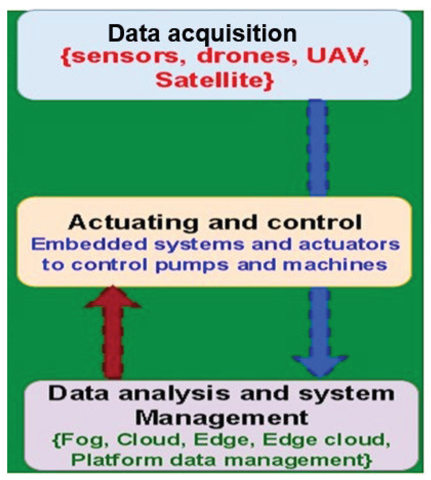
Figure 2.
WSN design approaches.
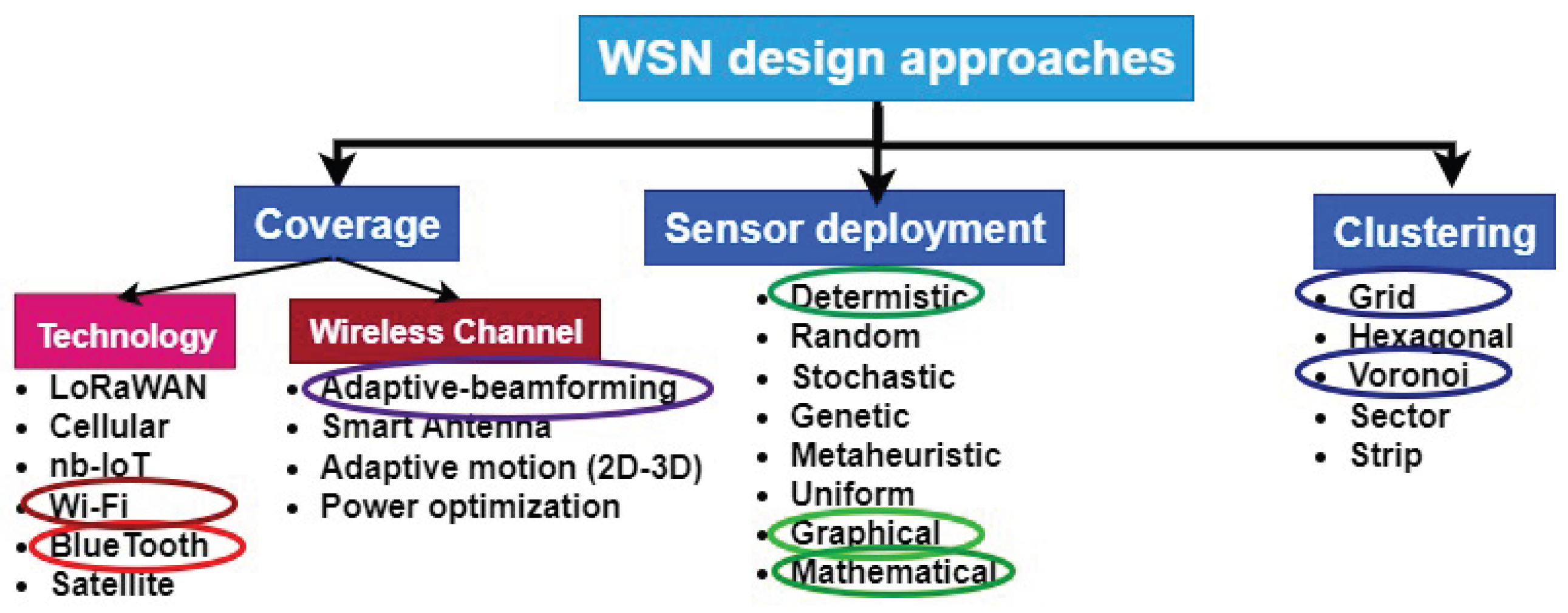
Figure 3.
Methodology.
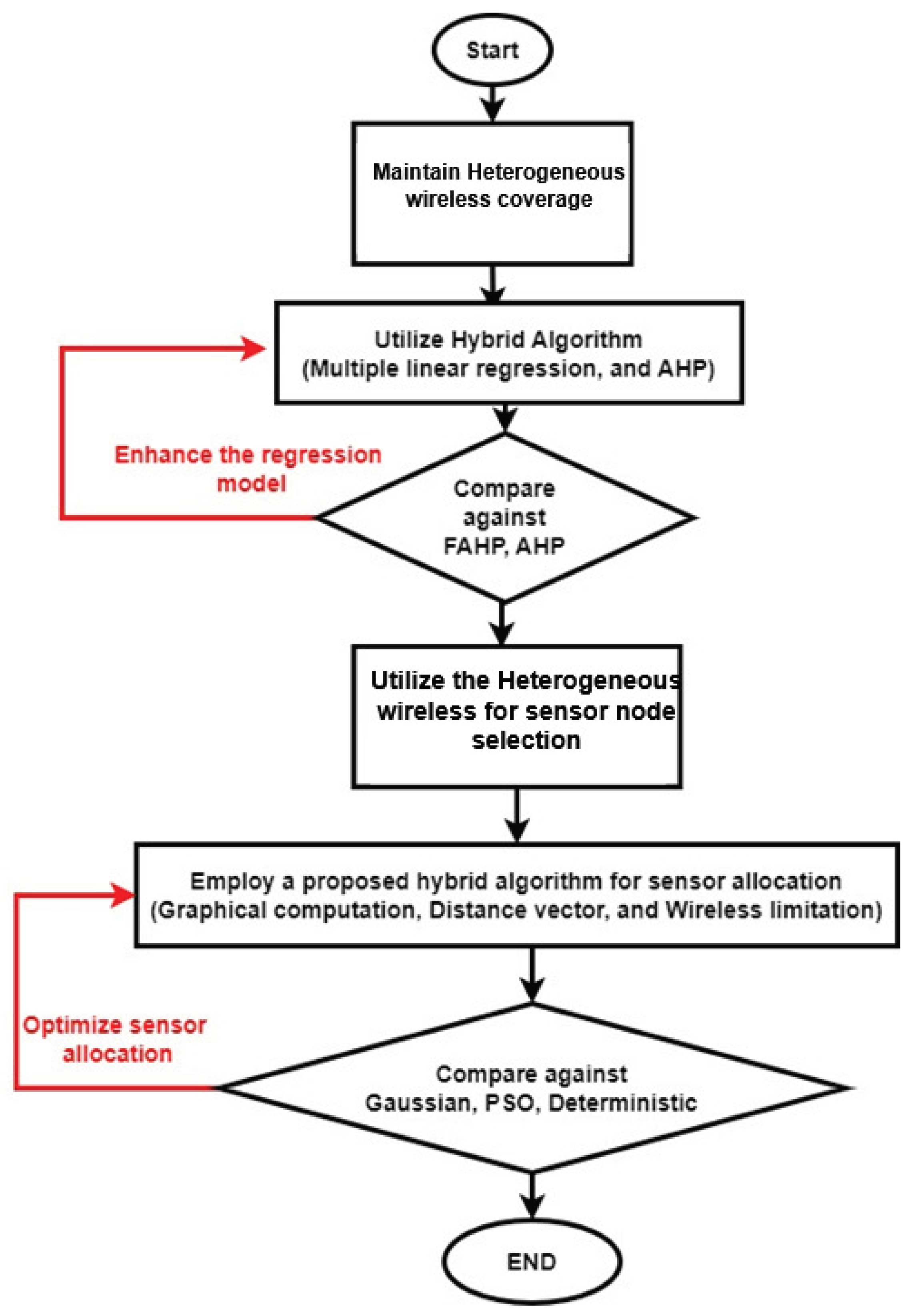
Figure 5.
Sensing Node schematic diagram.
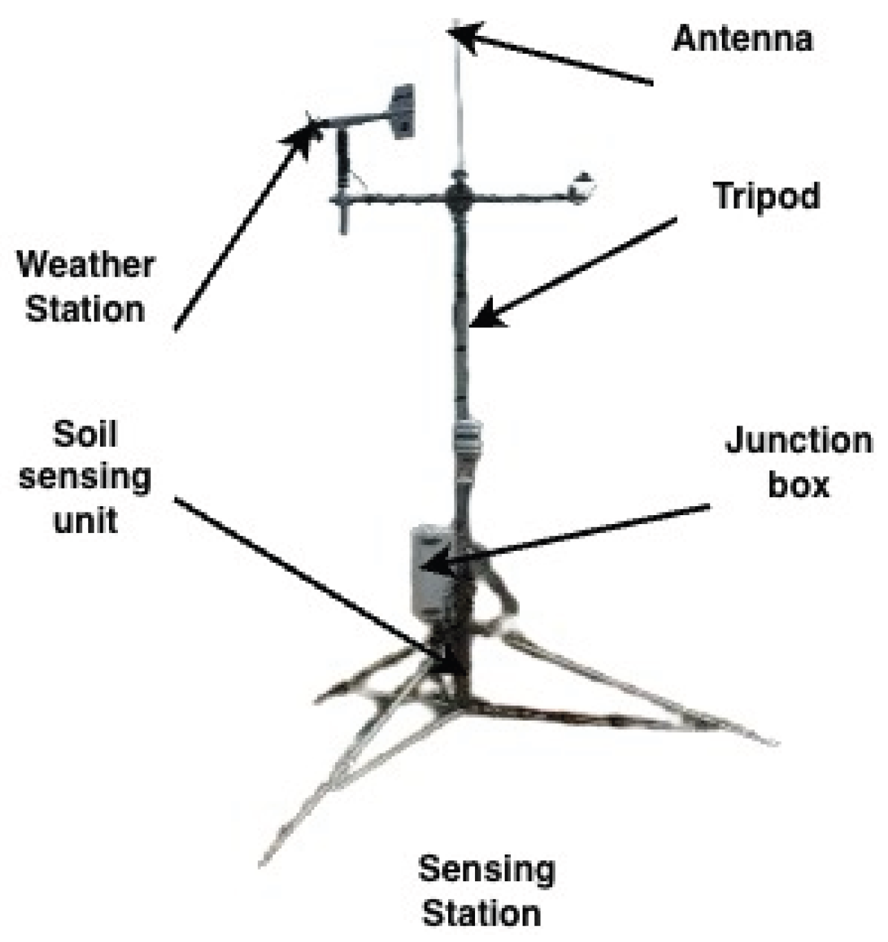
Figure 6.
Sensor allocation process flow chart.
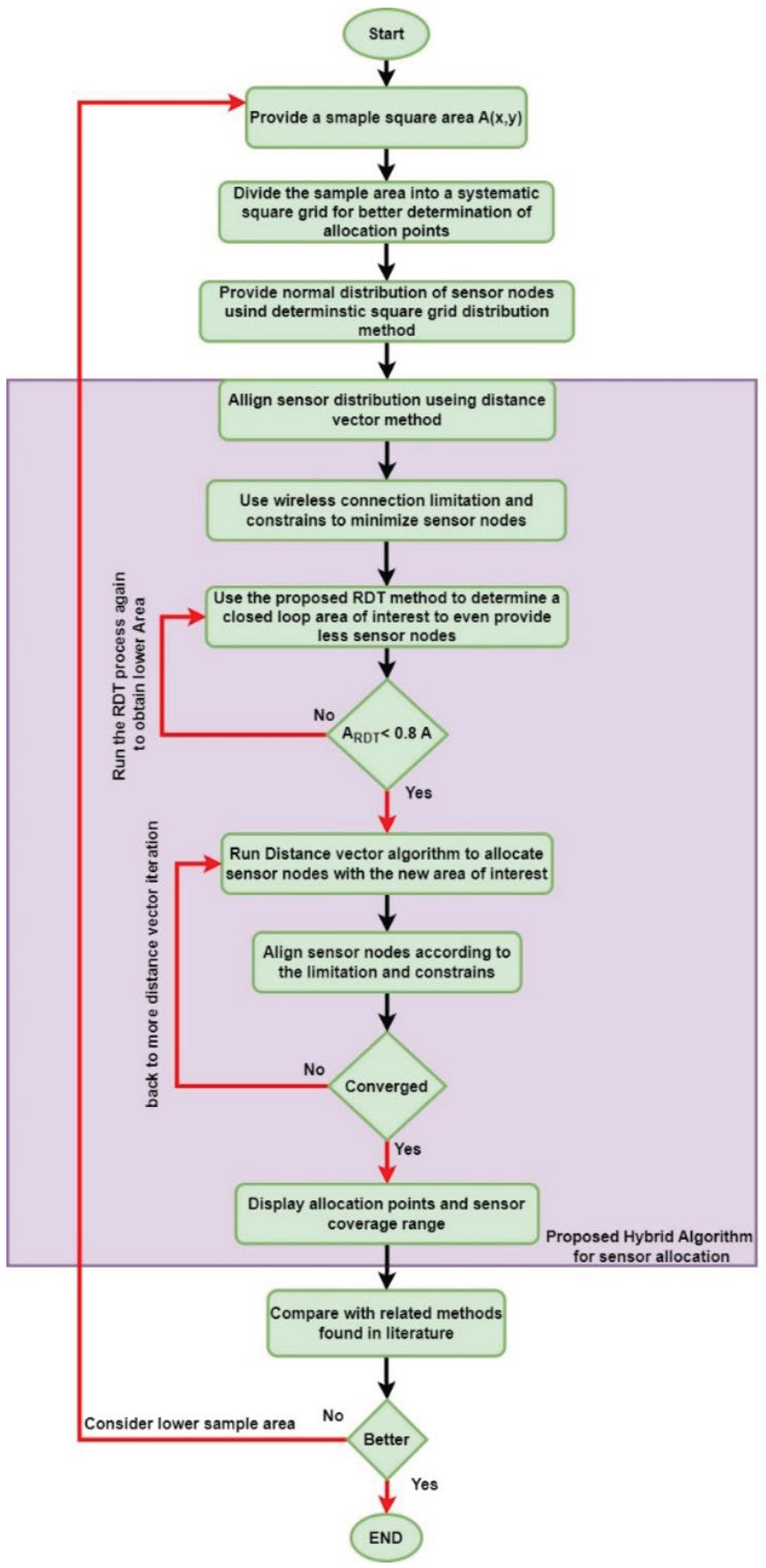
Figure 7.
Orchard sample area of systematic tree planting in a square grid scheme.
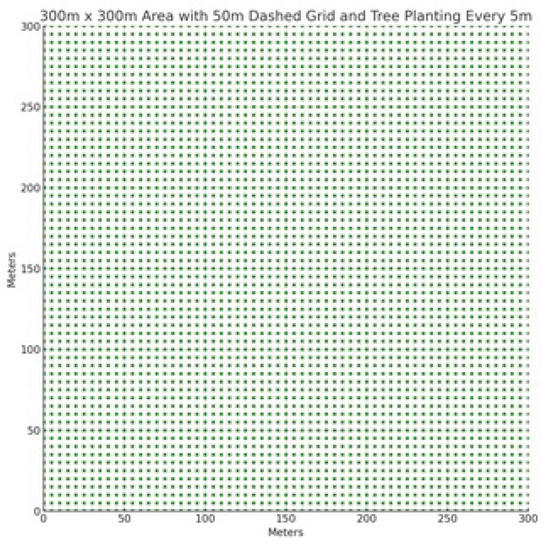
Figure 8.
Determining Maximum Distance for Wi-Fi Signal Extension: Key Practices.
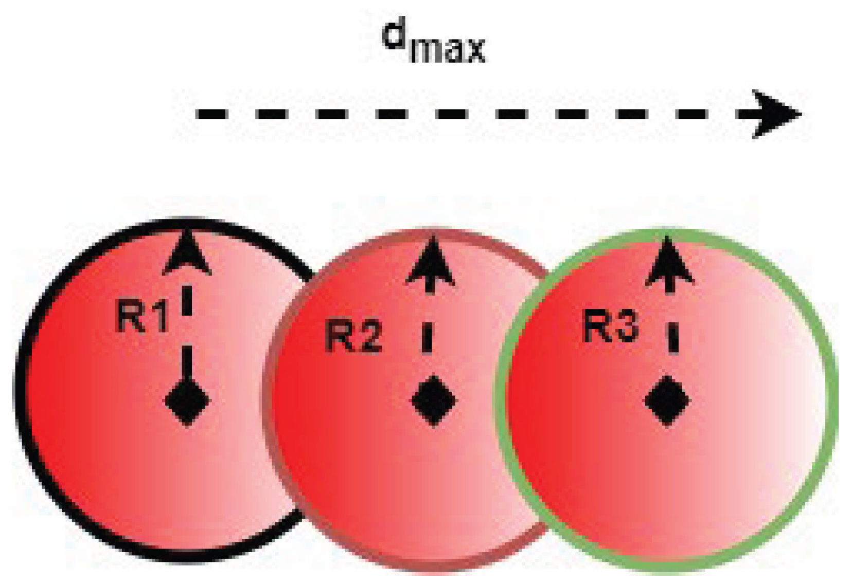
Figure 9.
Possible sensor allocation points.
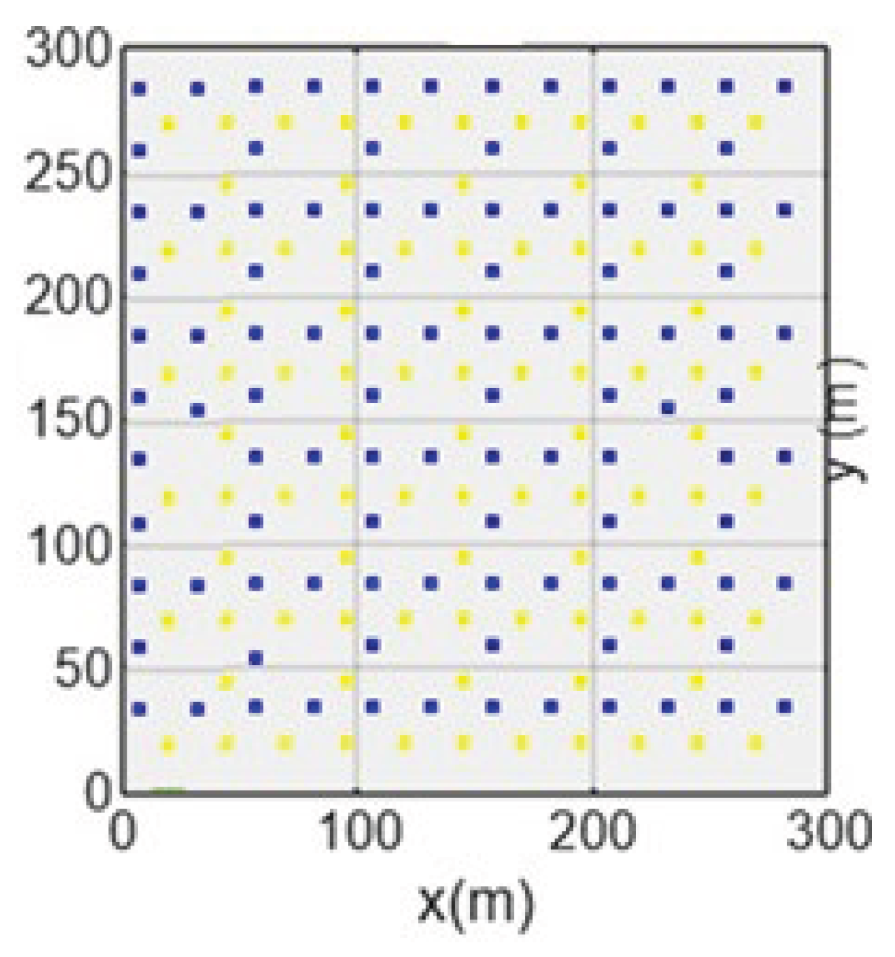
Figure 10.
Sensor node sensing and coverage limits.
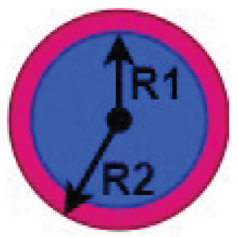
Figure 11.
Orchard field.
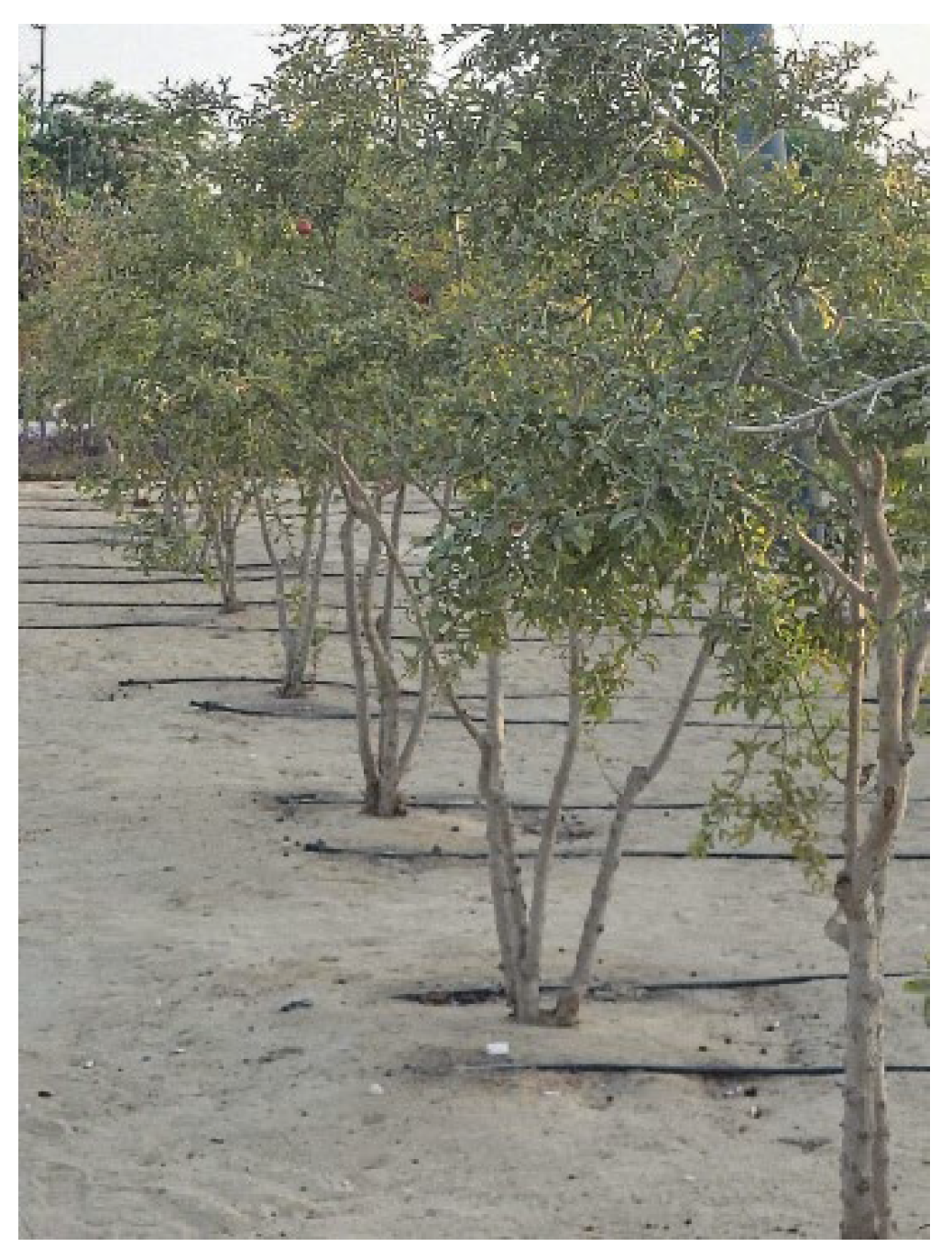
Figure 12.
Voronoi and adaptive beamforming pseudocode.
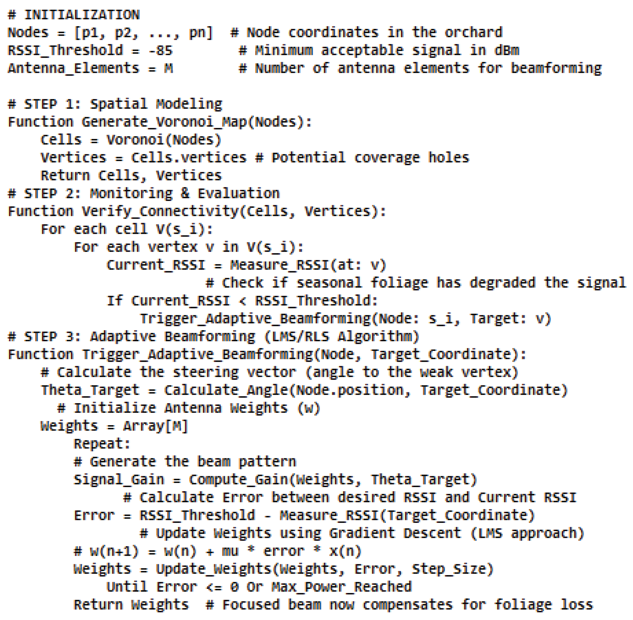
Figure 13.
Wireless networks evaluation with AHP.
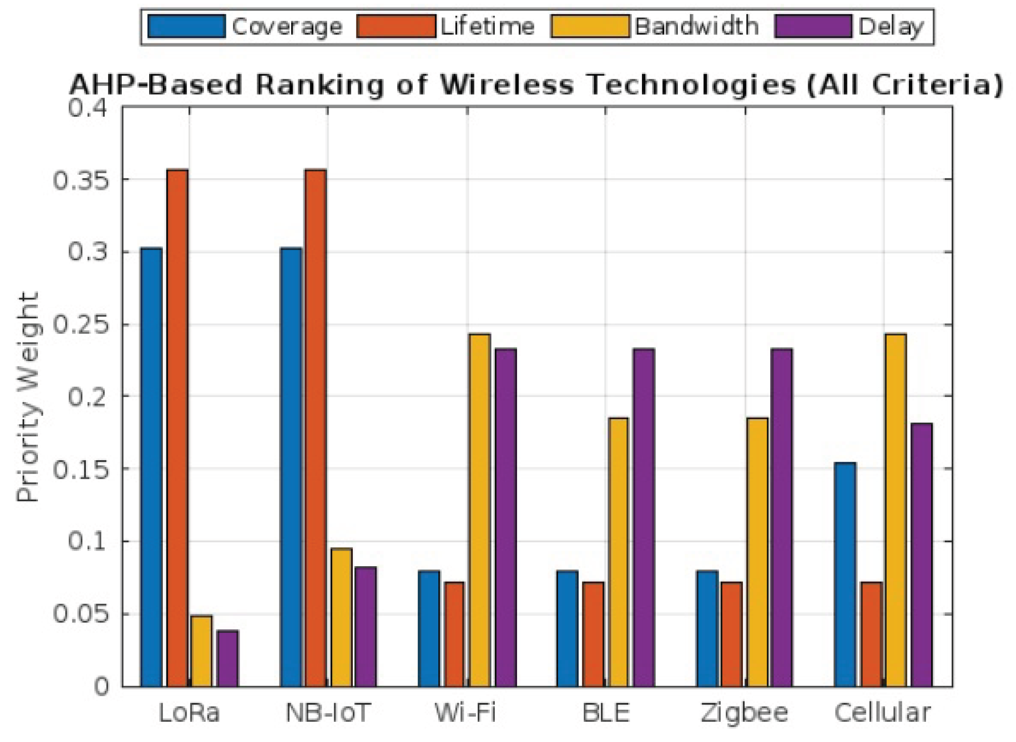
Figure 14.
Wireless evaluation related to the connectivity metric.
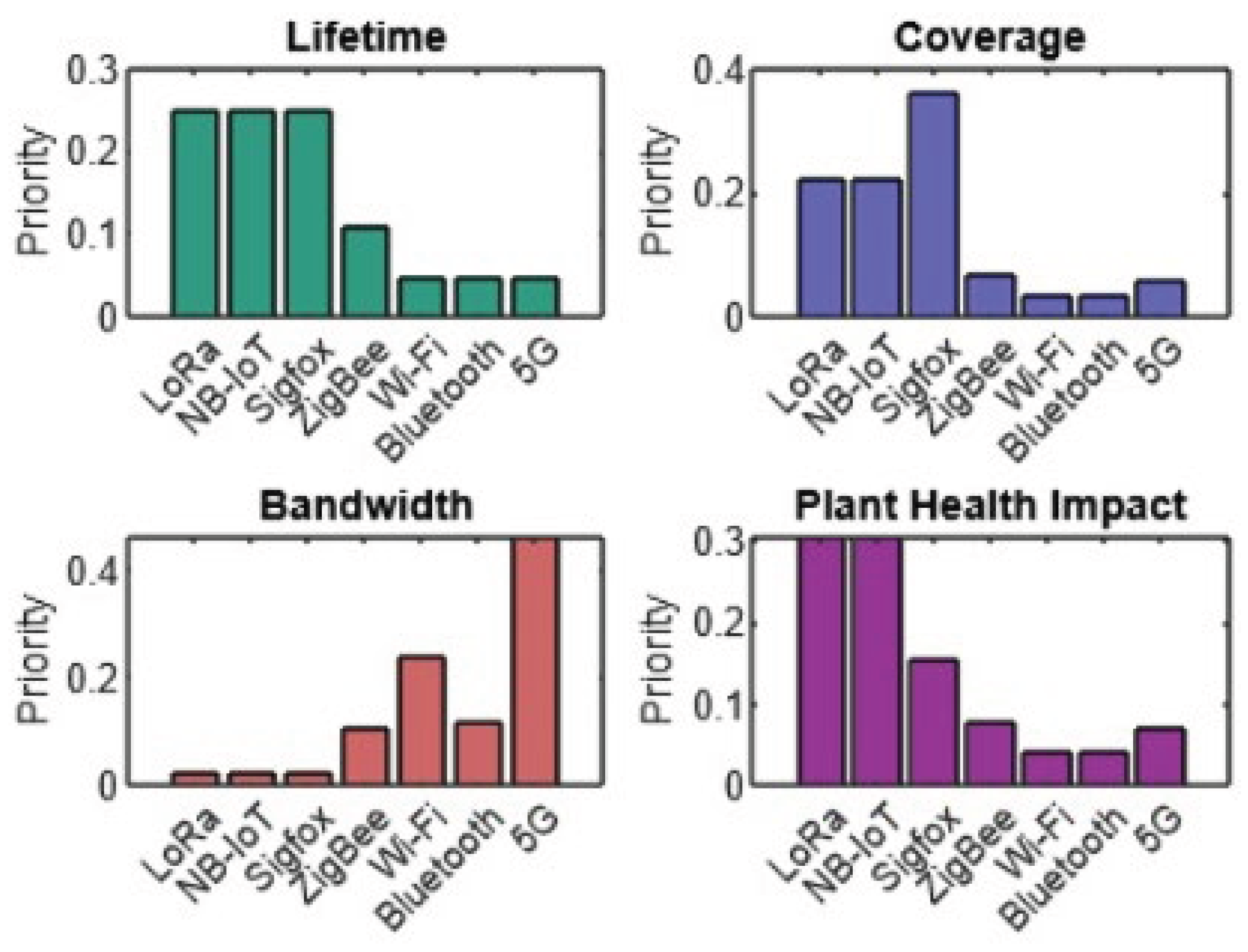
Figure 15.
Pairwise comparison matrix.
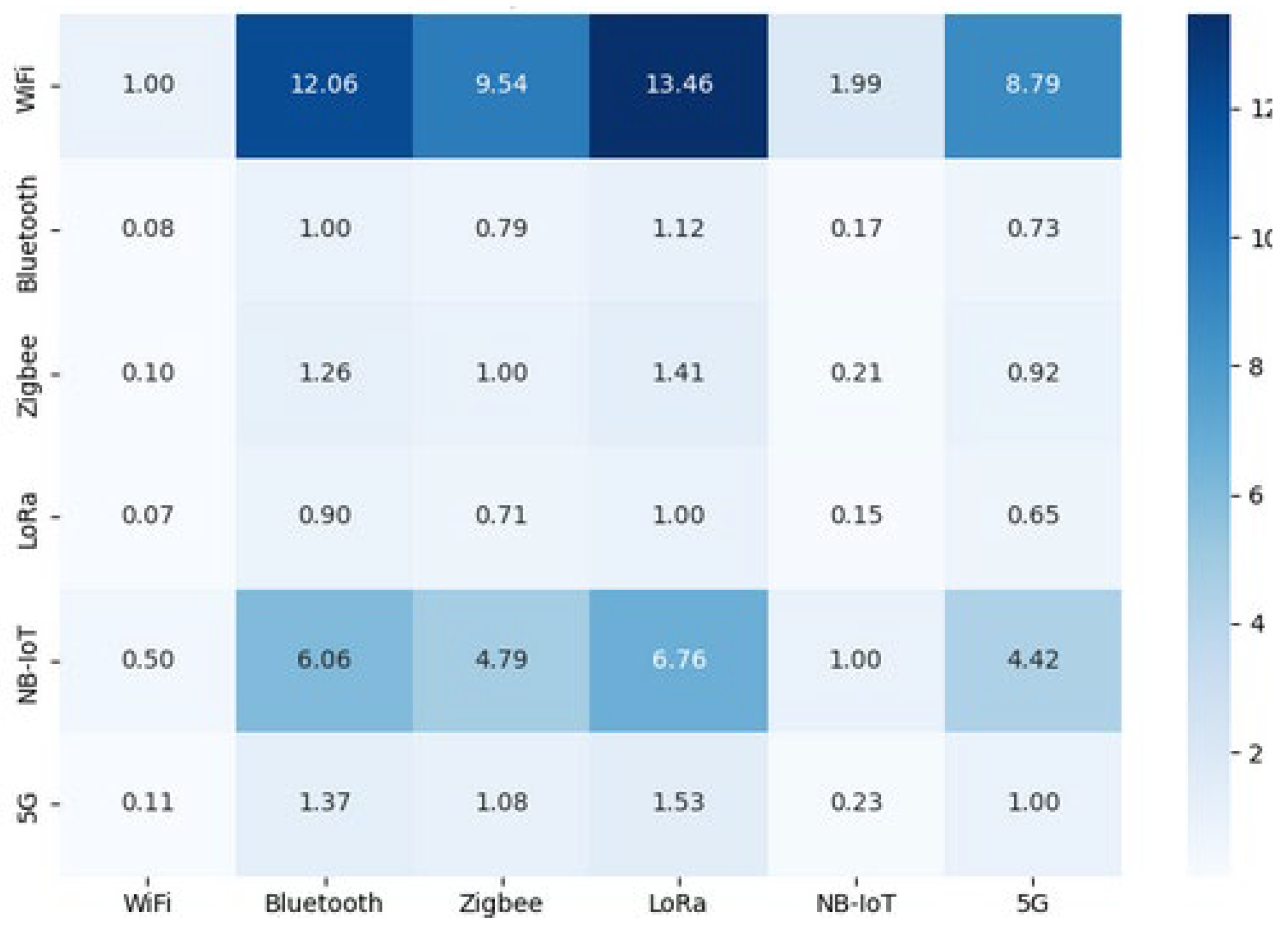
Figure 16.
Comparing the proposed MLR-AHP against AHP and FAHP.
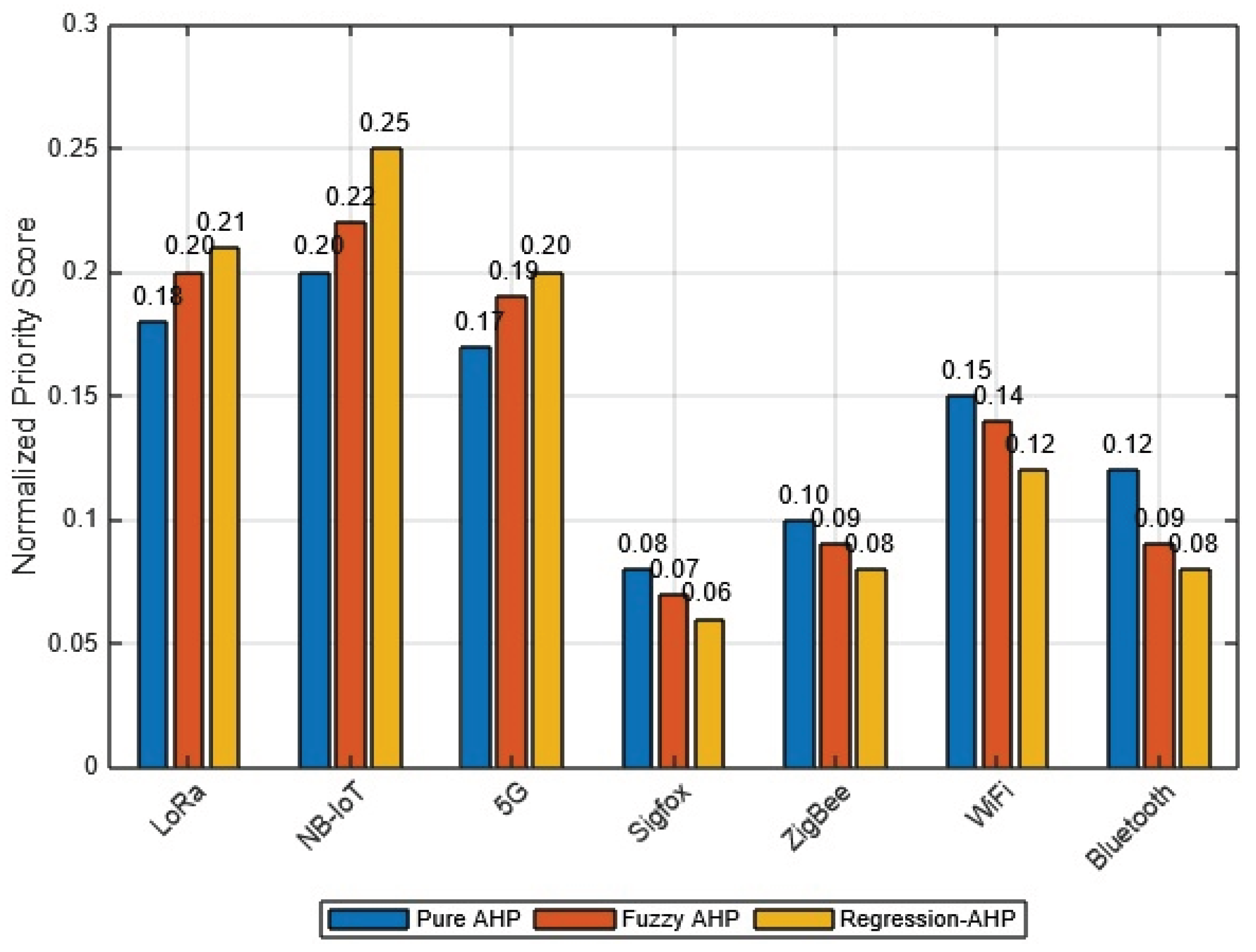
Figure 17.
Analysis of the three ranking methods.
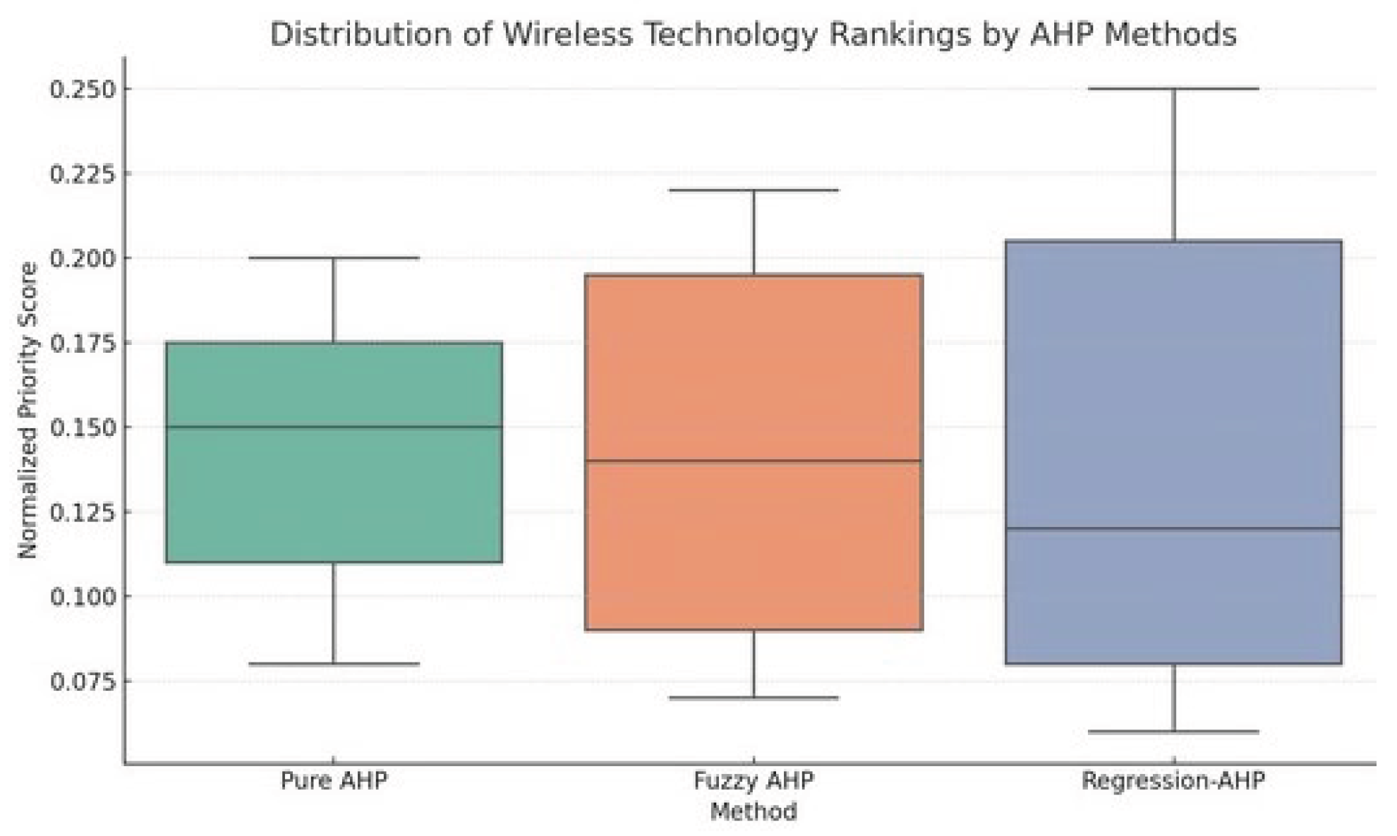
Figure 18.
Comparing the proposed solution against the prior solution.
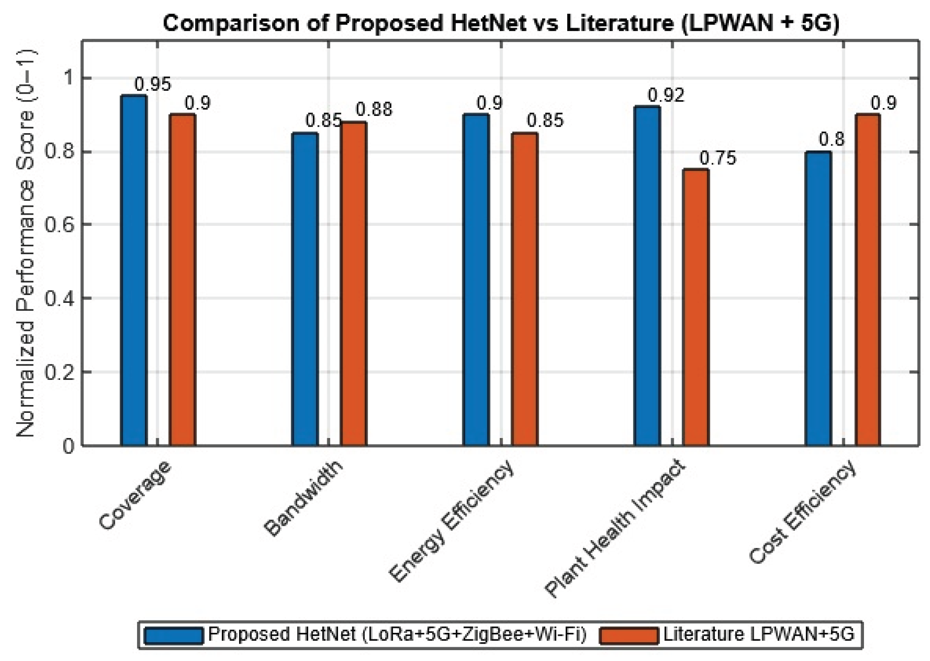
Figure 19.
Uniform sensor allocation.
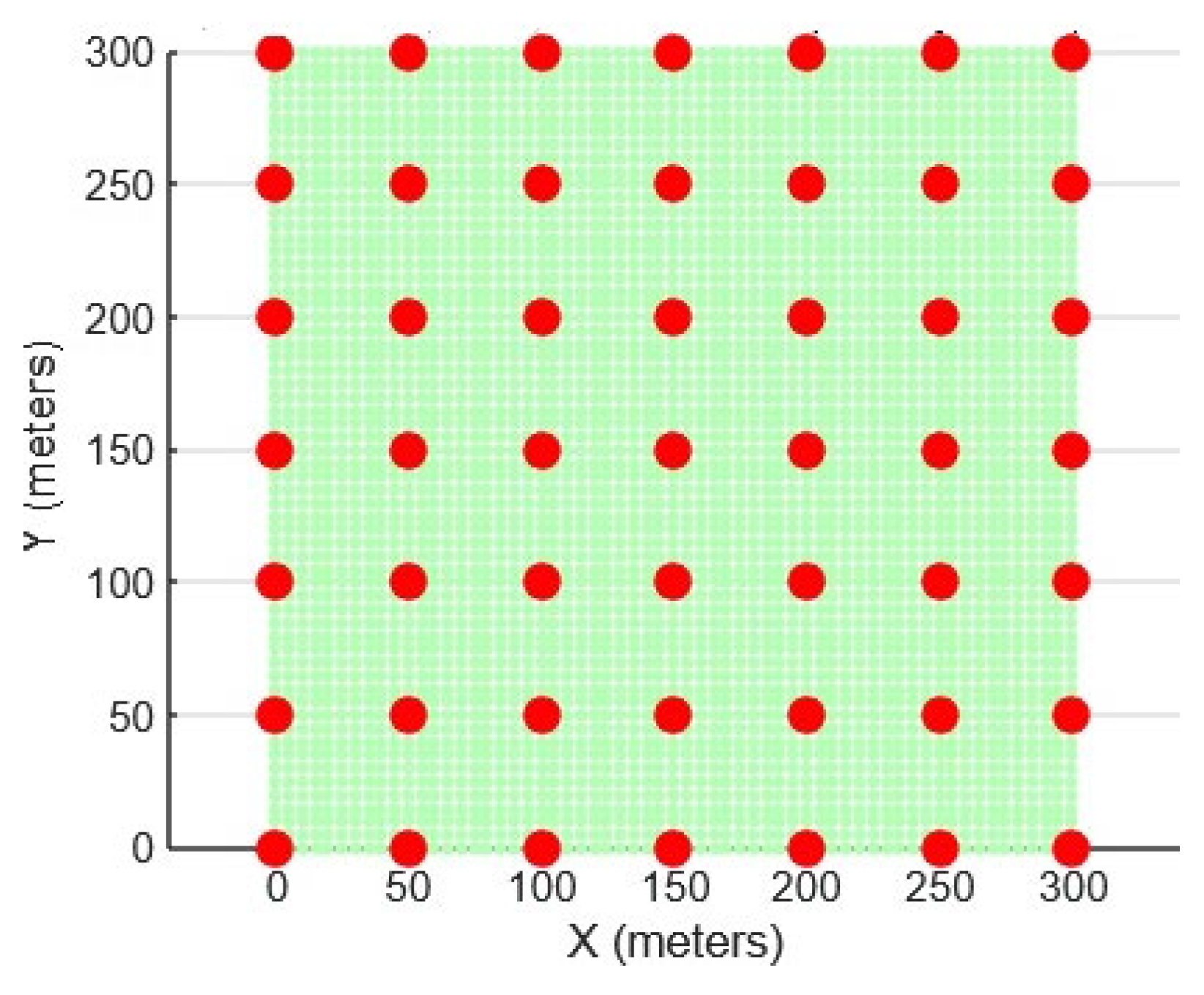
Figure 20.
Distance vector-assisted uniform sensor distribution.
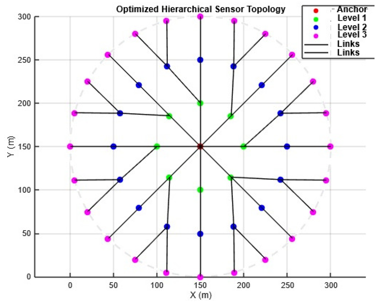
Figure 21.
Application of wireless limitations.
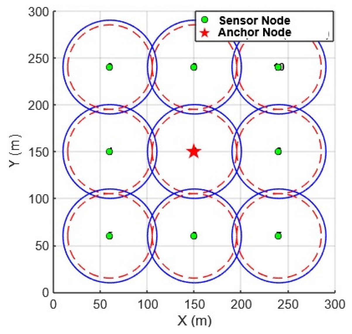
Figure 22.
Path planning using the RDT algorithm.
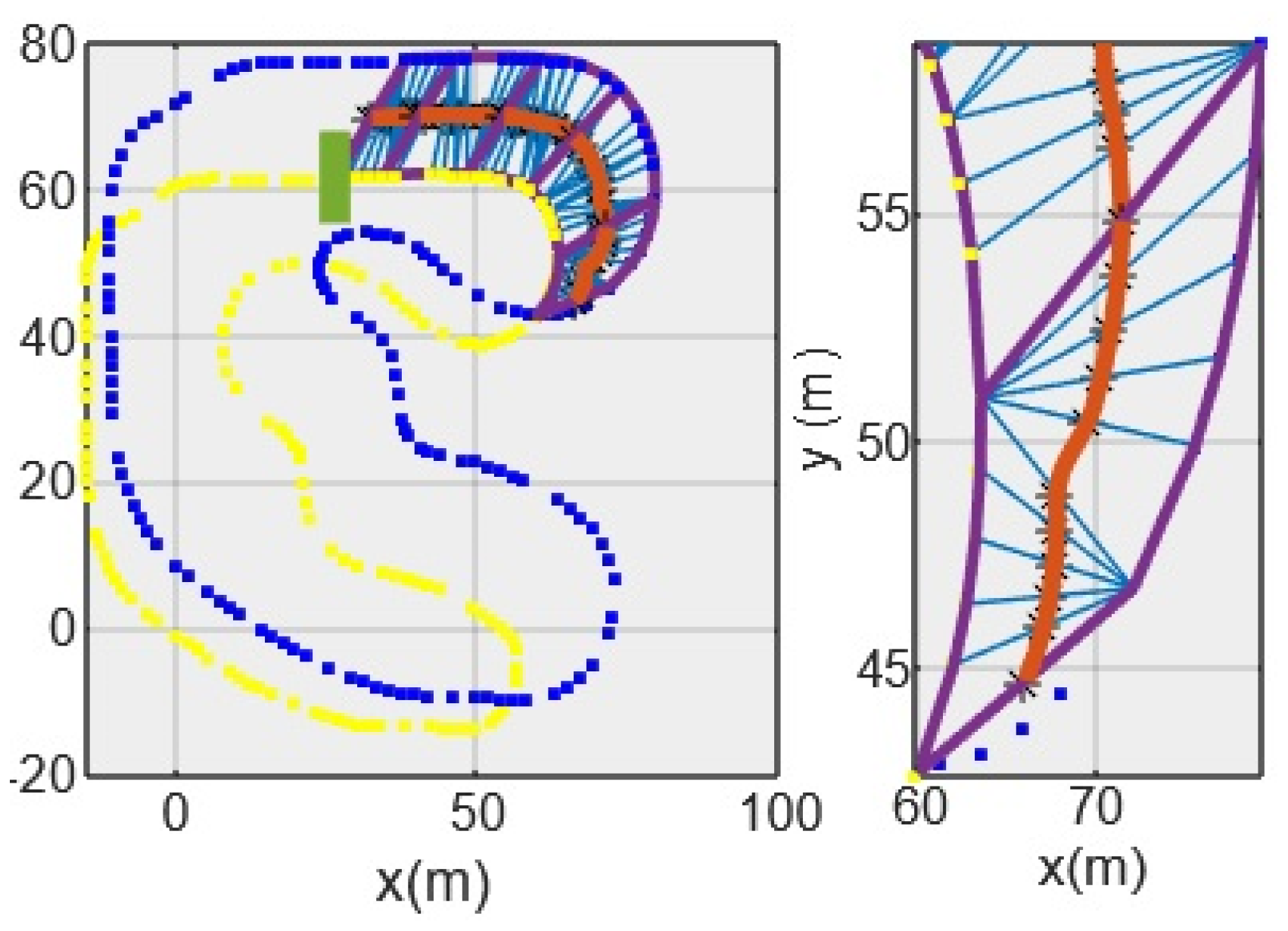
Figure 23.
Area of Interest assisted sensor distribution.
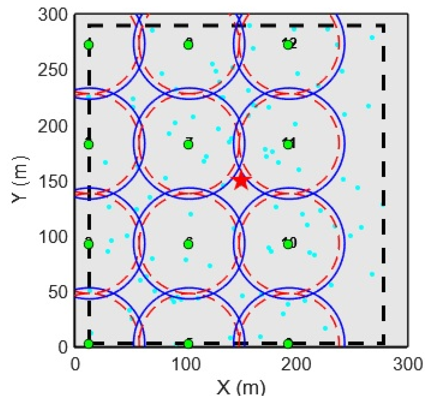
Figure 24.
Final sensor nodes reformation.
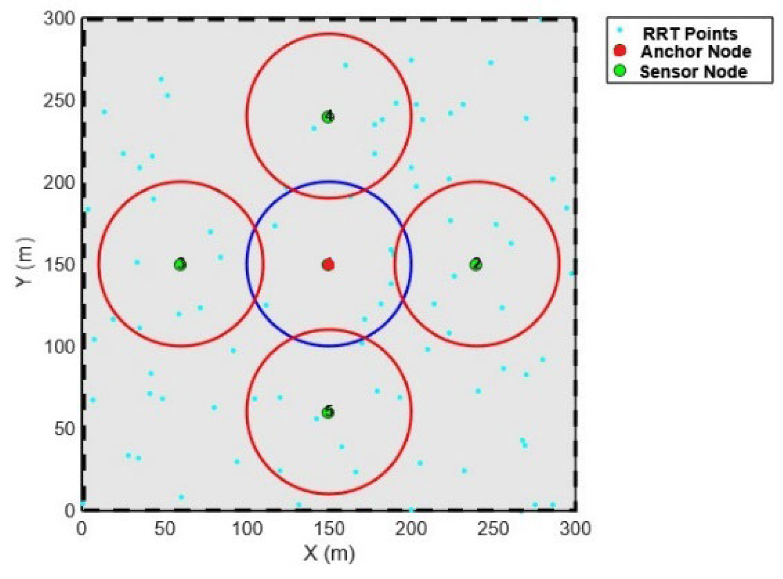
Figure 25.
Comparing methods based on coverage percentage.
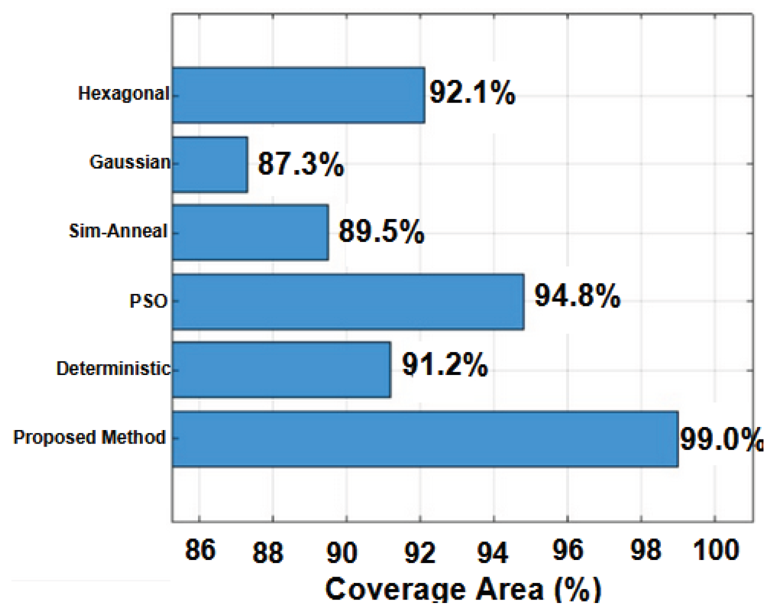
Figure 26.
Analysis of methods utilizing the heatmap method.
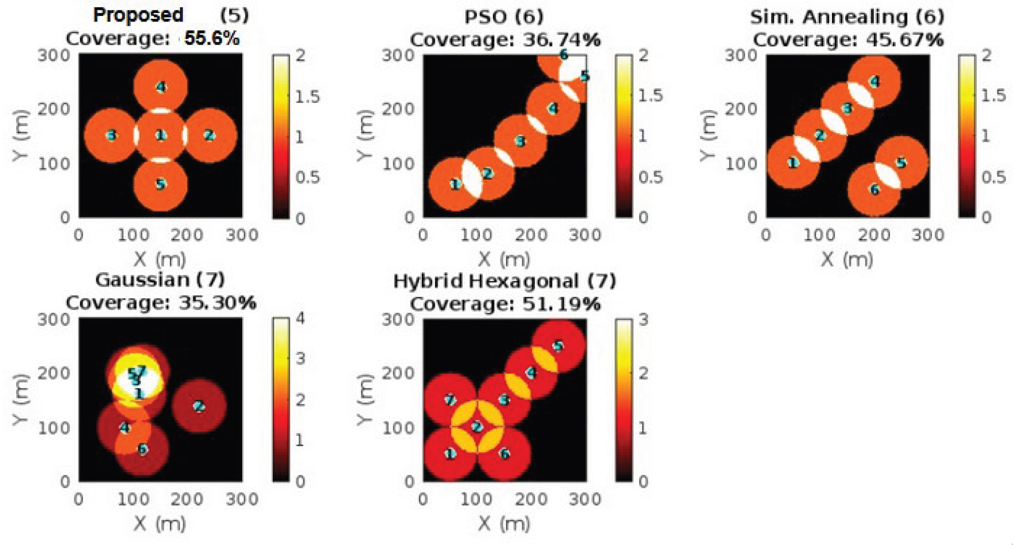
Figure 27.
Sensor node deployment comparison based on power consumption and latency.
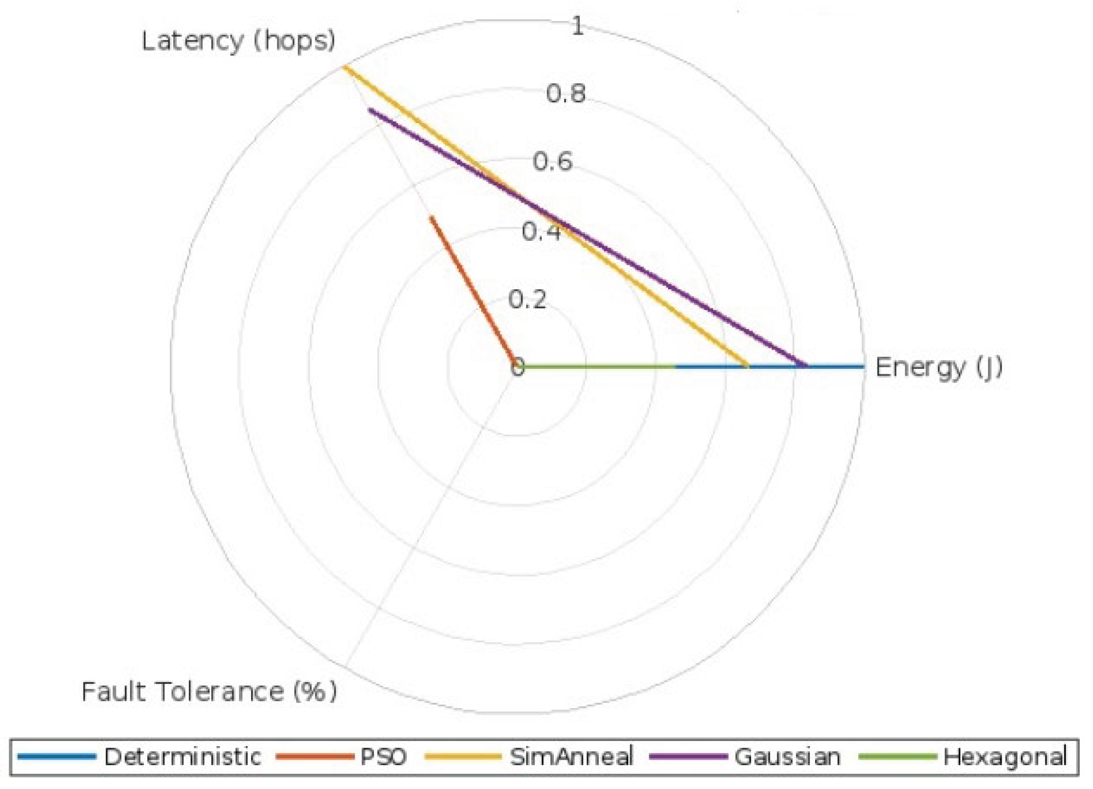
Figure 28.
Evaluating methods based on energy consumption.
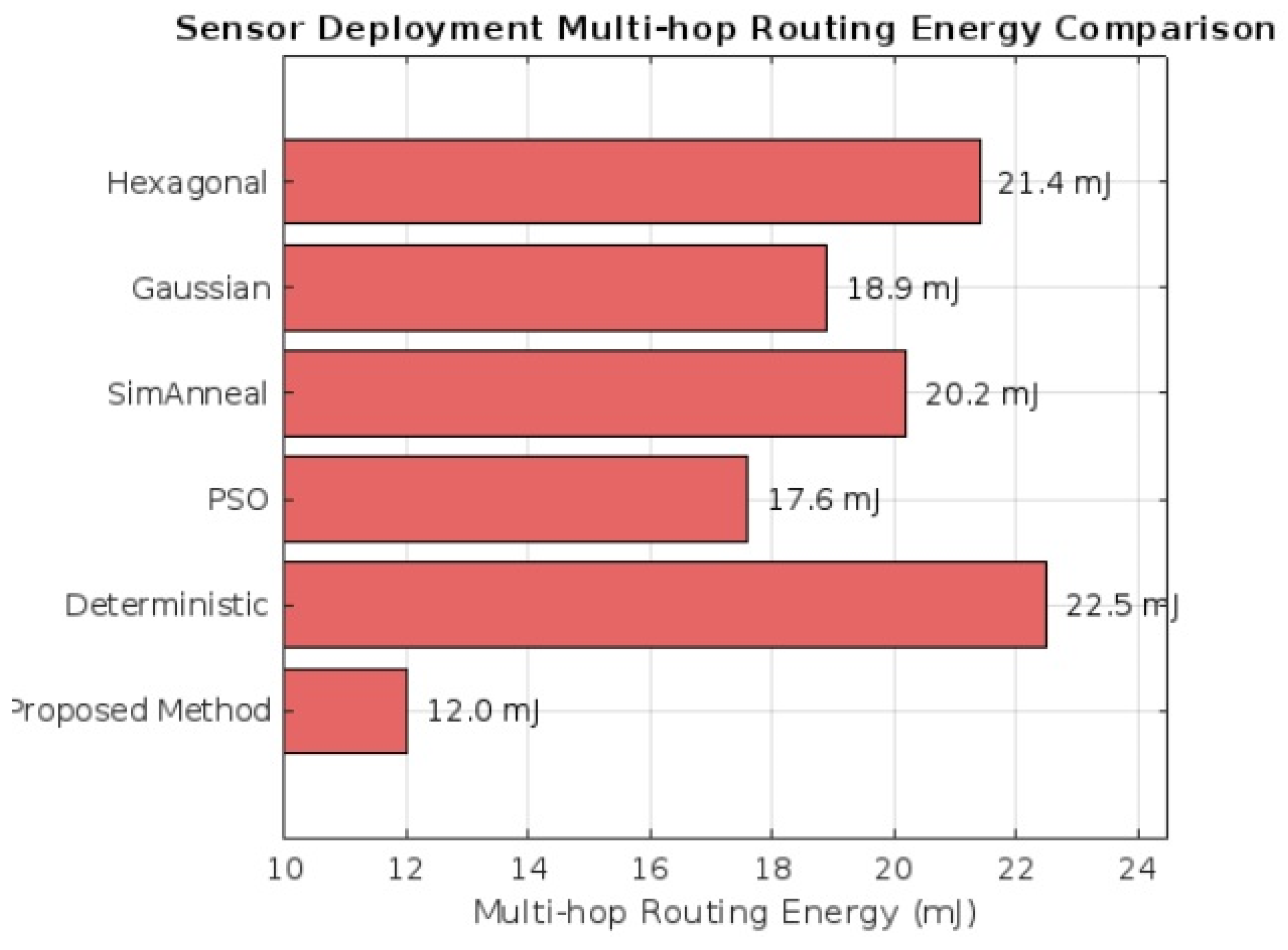
Figure 29.
Sensor allocation prototype.
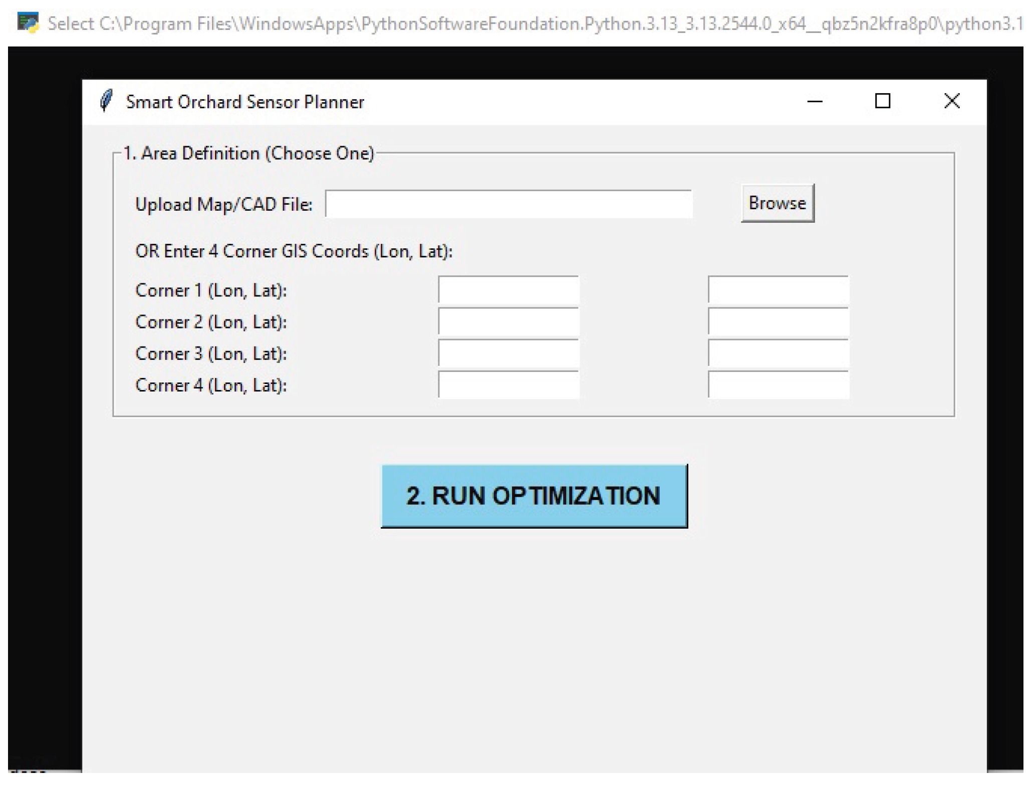
Figure 30.
Orchard Agriculture Area Image with Satellite.
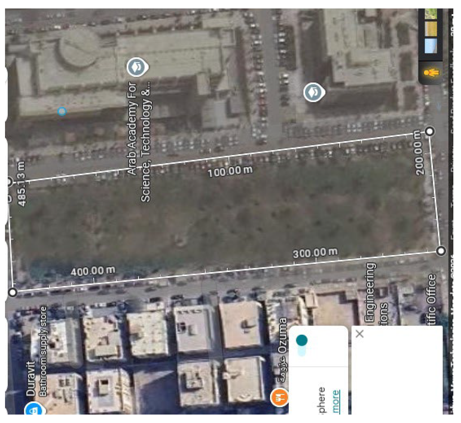
Figure 31.
Results of sensor allocation prototype.
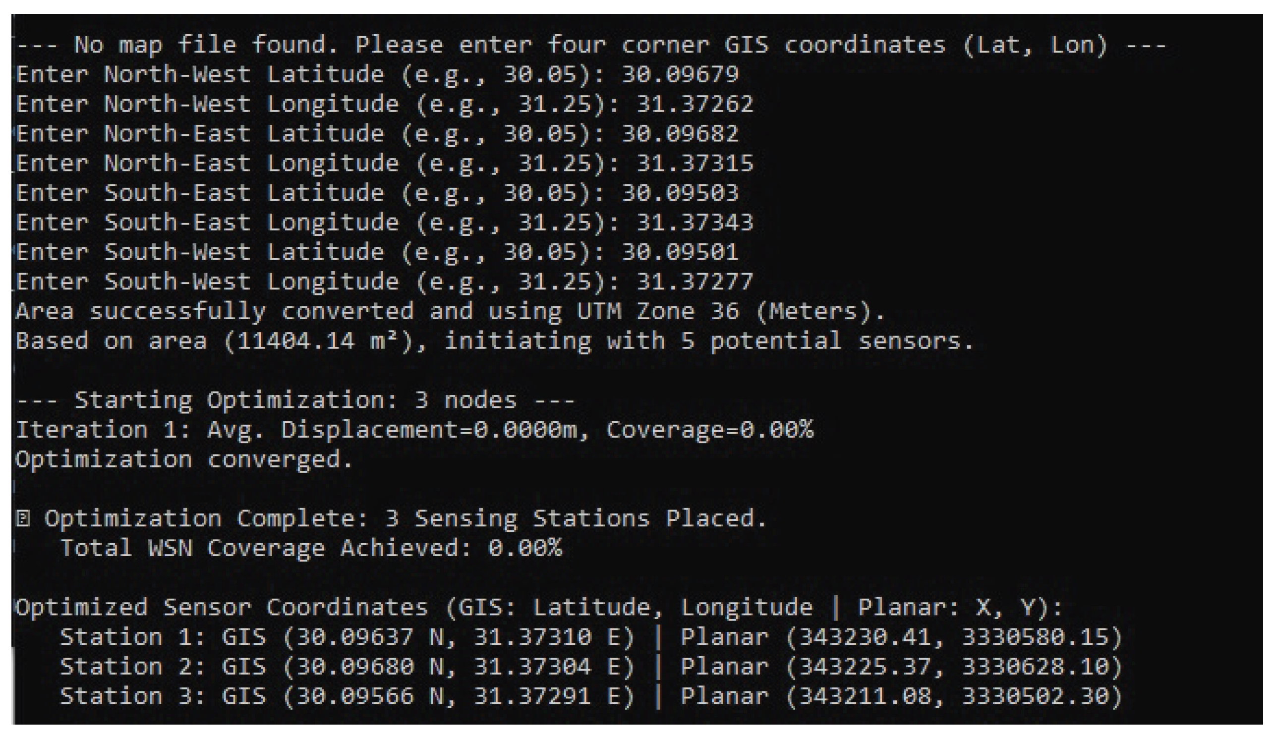
Figure 32.
GIS coordinates allocation and marking.
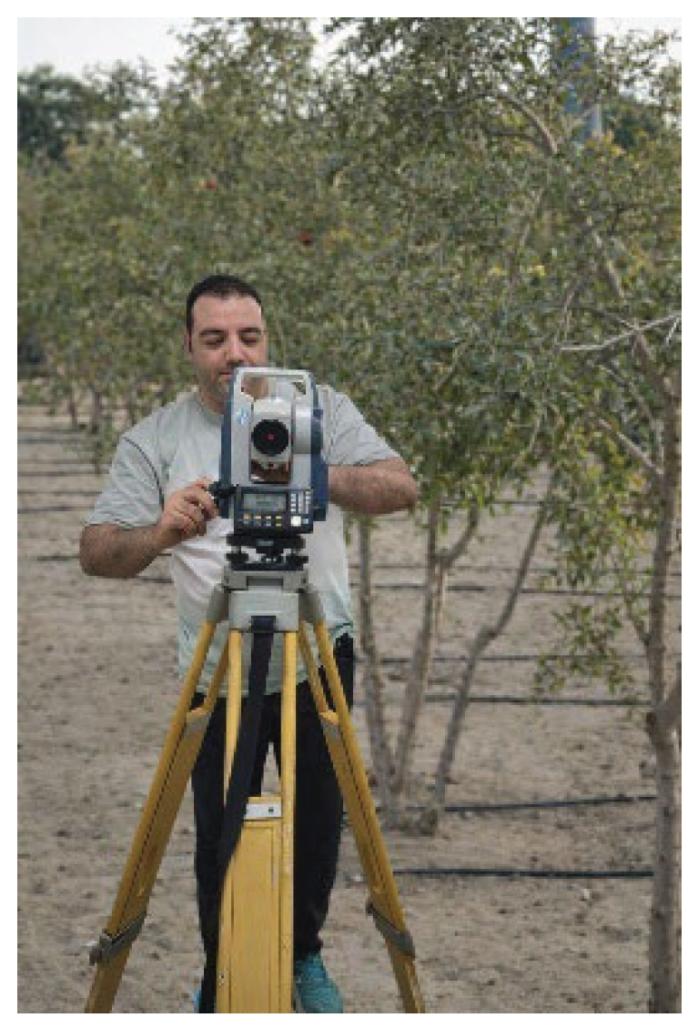
Figure 33.
Allocating sensor nodes through the garden.
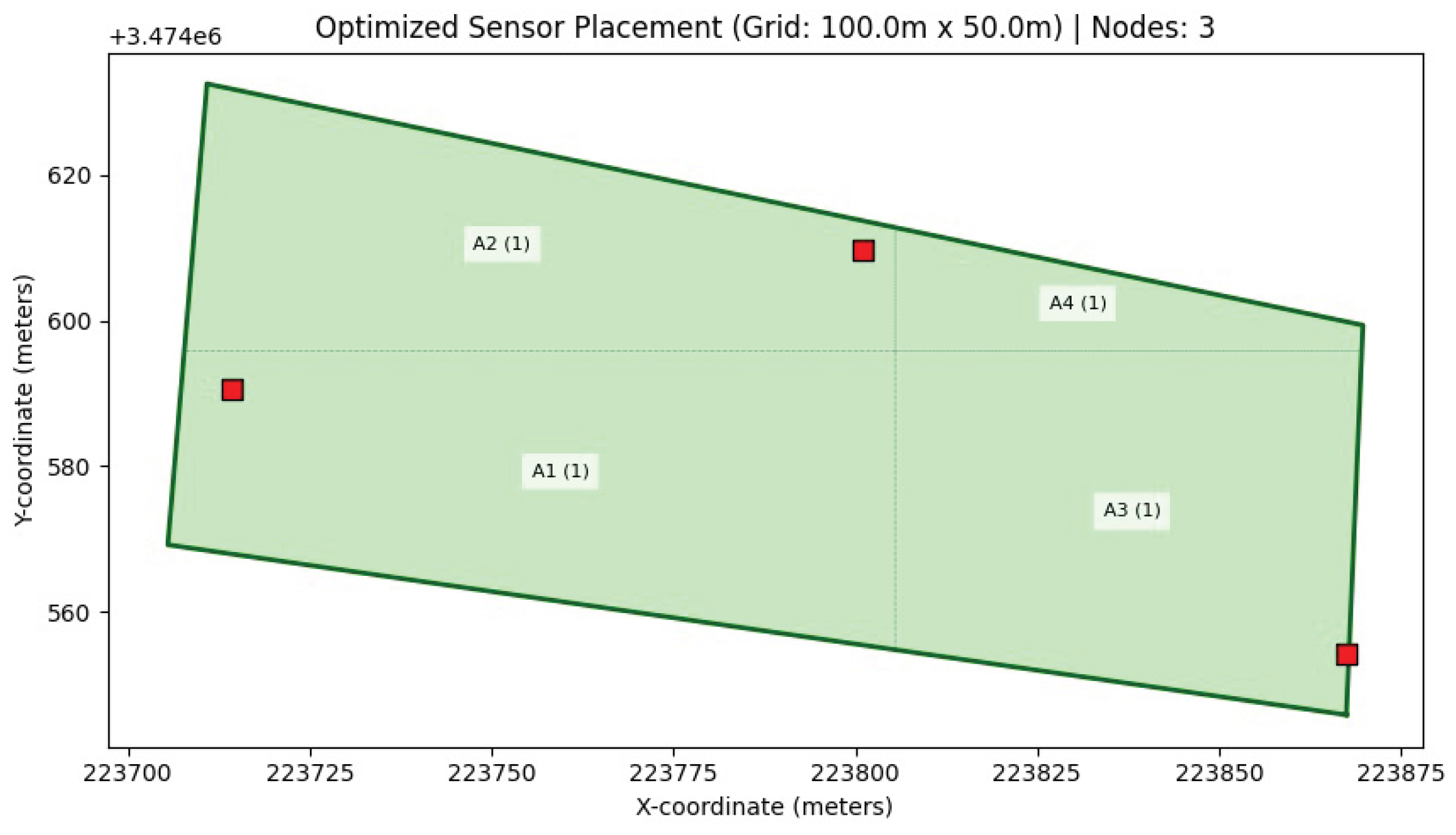
Figure 34.
Voronoi clustering and validation of sensing and covering.
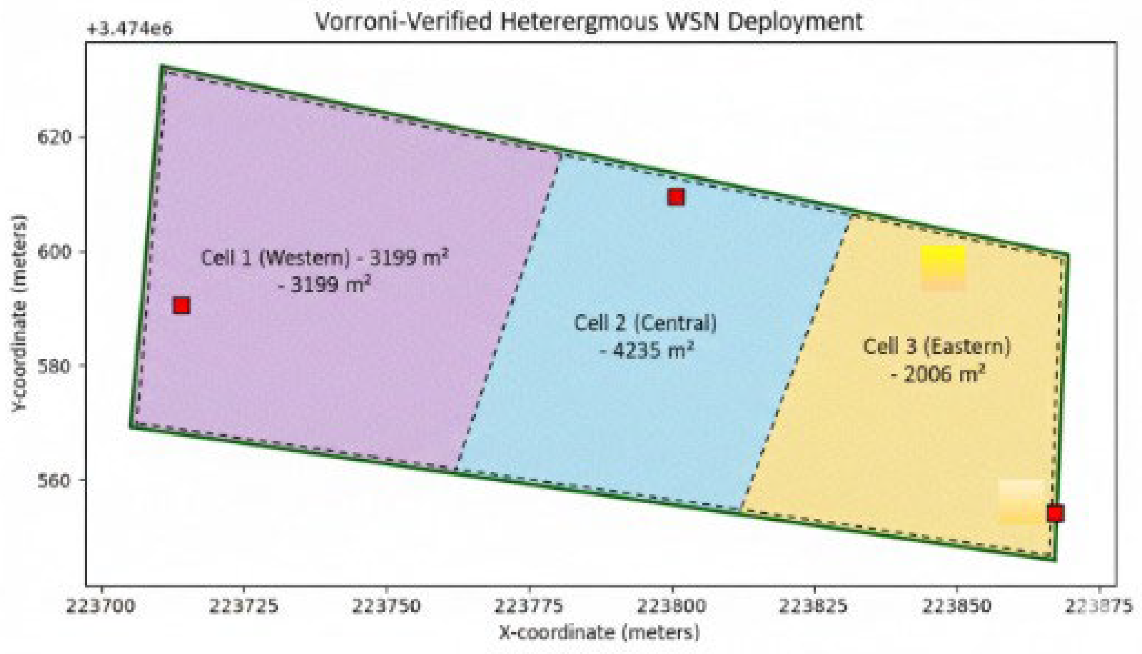
Figure 35.
RSSI based Adaptive beamforming improvement.
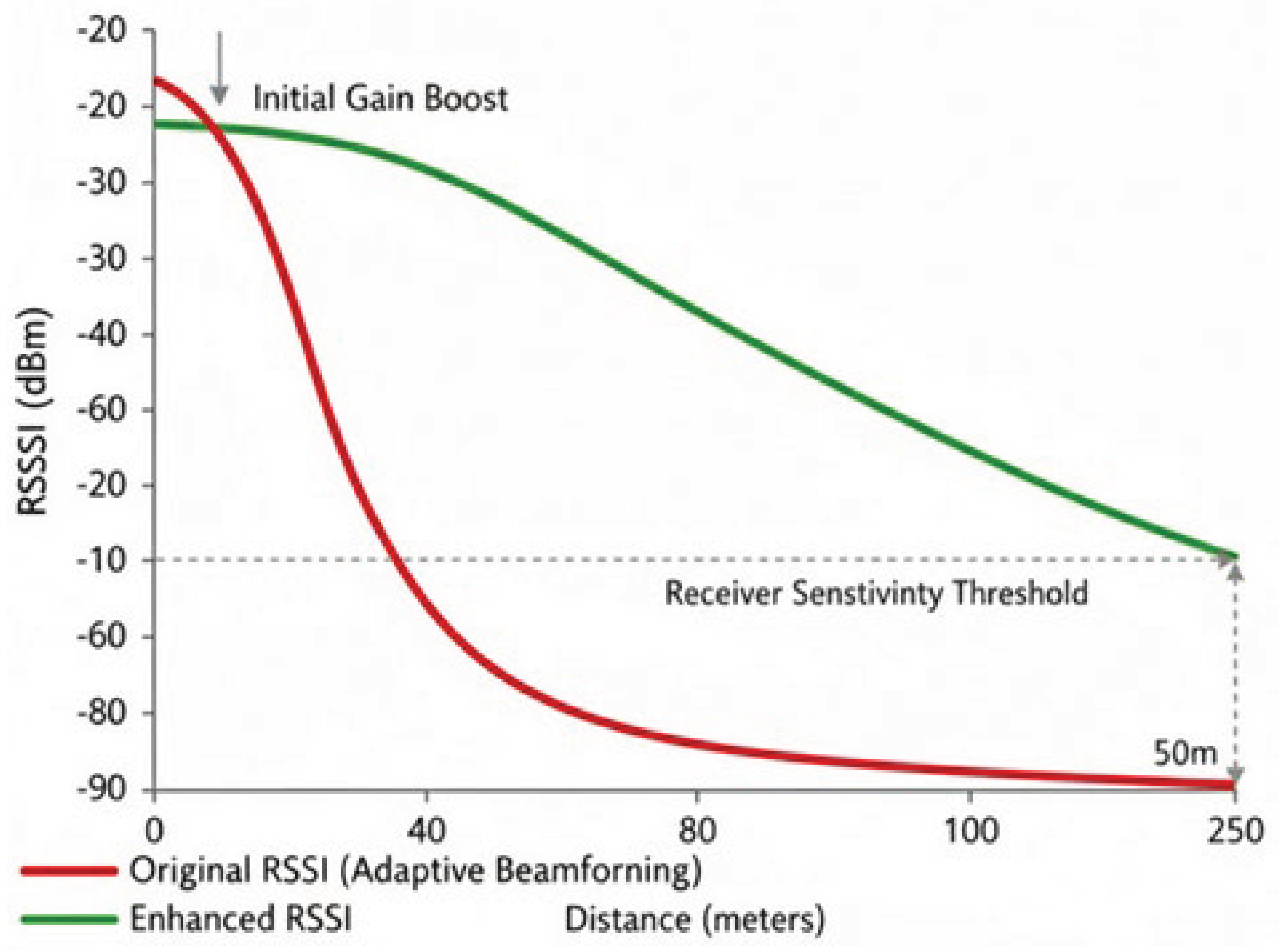

Table 1.
Values of the regression coefficients.
| Criterion | Coefficient (β) | Interpretation |
| Delay | -0.35 | Lower delay = better |
| Bandwidth | 0.30 | Higher bandwidth = better |
| Power | -0.15 | Lower power = better |
| Range | 0.10 | More range = slightly better |
| Plant Health | 0.05 | Slightly beneficial |
| Capacity | 0.25 | Large positive weight |
Table 2.
Wireless Technology Coverage.
| Technology | Normalized Range |
Normalized Capacity |
Composite |
|---|---|---|---|
| Sigfox | 1.00 | 0.15 | 0.575 |
| NB-IoT | 0.70 | 0.75 | 0.725 |
| LoRa | 0.20 | 0.15 | 0.175 |
| ZigBee | 0.002 | 1.00 | 0.501 |
| Wi-Fi | 0.002 | 0.003 | 0.002 |
| Bluetooth | 0.0002 | 0.0001 | 0.00015 |
Table 3.
Wireless Technologies Lifetime.
| Technology | Power (mw) | Lifetime Score (1/Power) |
| LoRa | 10 | 0.10 |
| NB-IoT | 20 | 0.05 |
| ZigBee | 40 | 0.025 |
| Sigfox | 50 | 0.02 |
| Blue | 100 | 0.01 |
| Wi-Fi | 500 | 0.002 |
Table 4.
Wireless Technologies: Plant Health Impact.
| Technology | 1/Delay | Impact | Score |
| Bluetooth | 0.200 | 4 | 2.80 |
| Wi-Fi | 0.100 | 3 | 1.80 |
| ZigBee | 0.010 | 6 | 3.00 |
| NB-IoT | 0.002 | 8 | 4.80 |
| LoRa | 0.001 | 9 | 5.40 |
| Sigfox | 0.0005 | 7 | 4.20 |
Table 5.
Bandwidth ranking.
| Technology | Bandwidth (kbps) |
| Wi-Fi | 54000 |
| Bluetooth | 1000 |
| ZigBee | 250 |
| NB-IoT | 250 |
| Sigfox | 100 |
| LoRa | 50 |
Table 6.
Sensor elements equipment for both sensor node types 1 and 2.
| physical Parameter | Sensor Type | Measurement Technique | Sensor Node Equipment |
Sensor vendor |
|---|---|---|---|---|
| Air Temperature & RH (Relative Humidity) |
Thermistor / Capacitive Polymer | Temperature: Change in resistance. Humidity: Change in the dielectric constant of a hygroscopic material | Type 1 &2. | Vaisala series, DHT22 [54] |
| Wind Speed & Direction | Anemometer (Cup/Propeller) | Cup/Propeller: Measures the rotation frequency. | Type 1. | Gill Instruments [55] |
| Precipitation | Tipping Bucket | Measures the number of tips (volume) of a small, calibrated bucket filled by rain. | Type 1. | Decagon [56] |
| Solar Radiation | Pyranometer | Pyranometer: Measures total (shortwave) radiation using a thermopile to detect heat generated by solar energy. | Type 1,2. | Apogee Instruments [57] |
| Soil Moisture | Capacitance | Type 1&2. | METER Group [58] | |
| Soil Electrical Conductivity (EC) | Four-Probe Method | Measures the soil's ability to conduct an electric current across electrodes. | Type 1. | METER [59] |
| Soil pH | Potentiometric | Measures the voltage potential. | Type 1. | METER [60] |
Table 7.
ANOVA simulation parameters.
| Method | Network | Coverage | Power Consumption | Bandwidth | Delay |
| AHP | Wi-Fi | 0.65 | 0.80 | 0.35 | 0.70 |
| FAHP | Wi-Fi | 0.68 | 0.82 | 0.38 | 0.65 |
| MLR-AHP | Wi-Fi | 0.75 | 0.78 | 0.45 | 0.60 |
| AHP | BLE | 0.0150 | 0.880 | 0.1800 | 0.240 |
| FAHP | BLE | 0.0100 | 0.100 | 0.1000 | 0.200 |
| Regression-AHP | BLE | 0.0180 | 0.982 | 0.1830 | 0.265 |
Disclaimer/Publisher’s Note: The statements, opinions and data contained in all publications are solely those of the individual author(s) and contributor(s) and not of MDPI and/or the editor(s). MDPI and/or the editor(s) disclaim responsibility for any injury to people or property resulting from any ideas, methods, instructions or products referred to in the content. |
© 2026 by the authors. Licensee MDPI, Basel, Switzerland. This article is an open access article distributed under the terms and conditions of the Creative Commons Attribution (CC BY) license (http://creativecommons.org/licenses/by/4.0/).
Copyright: This open access article is published under a Creative Commons CC BY 4.0 license, which permit the free download, distribution, and reuse, provided that the author and preprint are cited in any reuse.


