Meta-Analysis of Paired Binary Data with Unobserved Dependence: Insights from Laterality and Bilateralism in Anatomy

Vasileios Papadopoulos; Aliki Fiska

doi:10.20944/preprints202602.0571.v1

2. Materials and Methods

2.1. Paired Binary Data Structure and Notation

We consider an anatomic variant that may be present on the left side, the right side, on both sides, or on neither side of an individual. Each observation therefore consists of a paired binary outcome, reflecting the presence or absence of the variant on the left and right sides within the same individual.

For conceptual clarity, it is useful to distinguish three related but distinct levels of description: individual-level pairing, joint occurrence, and marginal prevalences.

At the individual level, left- and right-side observations are inherently paired, because they arise within the same body and are subject to shared developmental, genetic, and environmental influences. This pairing implies that left- and right-side occurrences cannot, in general, be treated as independent realizations.

At the population level, the paired structure can be summarized by the joint distribution of left- and right-side presence. This joint distribution specifies the proportions of individuals in whom the variant is absent bilaterally, present only on the left, present only on the right, or present on both sides. These four joint probabilities fully characterize laterality and bilateralism at the individual level.

In practice, however, most primary anatomic studies do not report this joint distribution. Instead, they typically report only marginal side-specific prevalences: the proportion of individuals in whom the variant is observed on the left side and the proportion in whom it is observed on the right side. These marginal quantities summarize how frequently the variant appears on each side considered separately, but they do not indicate whether left- and right-side occurrences arise in the same individuals.

This distinction is critical. Marginal prevalences alone do not determine how often a variant occurs bilaterally, nor how often left-only and right-only cases occur. Multiple joint distributions—corresponding to different degrees of within-individual dependence—can produce exactly the same marginal prevalences. Consequently, when joint left–right information is unreported, the individual-level structure underlying laterality and bilateralism is fundamentally unobserved.

Throughout this study, we explicitly distinguish between marginal side-specific prevalences and the unobserved joint distribution that links them. All subsequent modeling is built on this distinction. Formally, we denote by

p_{i j}

the joint probability that the variant is present (

i = 1

) or absent (

i = 0

) on the left side and present (

j = 1

) or absent (

j = 0

) on the right side. These four probabilities fully characterize the paired distribution, while the marginal prevalences reported in primary studies correspond to linear combinations of the

p_{i j}

.

2.2. Target Estimands: Laterality and Bilateralism

We focus on two co-primary endpoints that capture complementary aspects of anatomic variation: laterality and bilateralism. Although both depend on the same underlying joint distribution, they address different anatomical questions and behave differently when joint information is missing.

2.2.1. Laterality

Laterality concerns whether a variant preferentially affects one side of the body over the other at the individual level. In paired binary data, laterality is quantified using the paired odds ratio, which compares the frequency of individuals with right-only manifestation to the frequency of individuals with left-only manifestation.

Importantly, this measure depends exclusively on discordant individuals—those in whom the variant is present on one side but absent on the other. Bilateral cases do not contribute to laterality, because they exhibit no side preference within individuals. As a result, laterality reflects directional asymmetry rather than overall prevalence or symmetry.

When discordant counts are explicitly reported in primary studies, the paired odds ratio is directly identifiable without additional assumptions. When only marginal prevalences are reported, however, the number of discordant individuals cannot be determined without making an assumption about how probability mass is distributed between discordant and concordant outcomes. Laterality inference therefore becomes sensitive to assumptions about within-individual dependence.

2.2.2. Bilateralism

Bilateralism addresses a different anatomical question: how often a variant occurs symmetrically on both sides within the same individual. We quantify bilateralism using bilateral prevalence, defined as the proportion of individuals in whom the variant is present on both the left and right sides.

Bilateral prevalence is conceptually distinct from side-specific prevalence and from the prevalence of having the variant on at least one side. Whereas marginal prevalences describe how frequently a variant appears on each side separately, bilateral prevalence captures the tendency toward symmetric expression within individuals.

Because bilateral prevalence depends directly on the joint occurrence of left and right manifestations, it cannot be inferred from marginal prevalences alone when joint data are unreported. Any estimate of bilateral prevalence under such conditions necessarily relies on an assumption about the underlying left–right dependence structure.

Taken together, laterality and bilateralism provide a complete and anatomically meaningful summary of paired binary variation. Laterality captures directional asymmetry among discordant individuals, whereas bilateralism captures symmetric expression among concordant individuals. The remainder of the Methods section develops a principled framework for analyzing both endpoints when the joint distribution underlying these quantities is unobserved.

2.3. Feasible Joint Distributions

When joint left–right data are unreported, the central inferential difficulty is that the joint distribution linking left- and right-side occurrences is unknown. However, it is not unconstrained. For any given pair of marginal side-specific prevalences, only a restricted set of joint distributions is mathematically admissible.

This restriction arises because joint probabilities must be non-negative, sum to one, and reproduce the observed marginal prevalences. As a consequence, the probability that a variant occurs bilaterally cannot vary freely: it is bounded above and below by limits determined entirely by the marginals. These limits are known as the Fréchet bounds.

Conceptually, the Fréchet bounds define the most extreme joint structures that are compatible with the observed marginals. At one extreme, left and right occurrences are arranged so as to minimize bilateral co-occurrence, subject to the marginal constraints. At the other extreme, left and right occurrences are arranged to maximize bilateral co-occurrence. Any joint distribution consistent with the reported marginals must lie between these two extremes.

The lower bound corresponds to the weakest possible within-individual association compatible with the marginals, while the upper bound corresponds to the strongest possible association. Importantly, neither bound generally corresponds to independence unless the marginals are balanced in a particular way. Independence is therefore one admissible joint structure, but not a privileged one.

Because laterality and bilateral prevalence both depend on how probability mass is allocated between concordant and discordant outcomes, their values are constrained by the same feasibility limits. When only marginal prevalences are known, neither laterality nor bilateral prevalence is identifiable without an additional assumption specifying where the true joint distribution lies within the admissible range.

This observation is fundamental. It implies that the inferential problem posed by unreported joint data is not one of estimation error, but of non-identifiability. Multiple, mutually incompatible joint distributions can reproduce the same marginal prevalences while implying different values of laterality and bilateral prevalence. Any analysis based on marginal data alone must therefore make an explicit assumption about the within-individual dependence structure.

In the following section, we make these feasibility constraints explicit by expressing the Fréchet bounds as inequalities on the joint probabilities and introducing a scalar parameter that spans the entire admissible dependence range.

2.4. Feasibility-Based Dependence Parameterization

As established in Section 2.3, when only marginal side-specific prevalences are available, the joint left–right distribution is not identifiable but is constrained to lie within a well-defined feasible region. We now formalize these constraints and introduce a scalar parameter that spans the entire admissible range of within-individual dependence.

Let

L

and

R

denote binary indicators of variant presence on the left and right sides, respectively, with joint probabilities

p_{i j} = P r (L = i, R = j), i, j \in {0,1} .

The marginal prevalences are given by

p_{L} = P r (L = 1) = p_{10} + p_{11}, p_{R} = P r (R = 1) = p_{01} + p_{11} .

Because probabilities must be non-negative and sum to one, the joint probability of bilateral occurrence

p_{11}

cannot take arbitrary values once

p_{L}

and

p_{R}

are fixed. Instead, it is constrained by the Fréchet bounds,

m a x {0, p_{L} + p_{R} - 1} \leq p_{11} \leq m i n {p_{L}, p_{R}} .

These bounds are sharp: every value of

p_{11}

within this interval corresponds to at least one valid joint distribution consistent with the observed marginals, whereas values outside the interval are mathematically impossible. Independence corresponds to the specific interior value

p_{11} = p_{L} p_{R}

, which is admissible but not privileged.

The Fréchet bounds therefore define a one-dimensional feasible segment of joint distributions compatible with the observed marginals. Any assumption about within-individual dependence in the absence of joint data amounts to selecting a point along this segment.

To parameterize this selection transparently, we introduce a feasibility-based dependence index

λ \in [0,1]

, defined through the linear interpolation

p_{11} (λ) = (1 - λ) p_{L} p_{R} + λ m i n {p_{L}, p_{R}} .

Under this construction,

λ = 0

corresponds to independence, while

λ = 1

corresponds to maximal feasible bilateral concordance. Intermediate values of

λ

span the entire admissible dependence range, ensuring that all assumed joint distributions are feasible for the observed marginals.

Once

p_{11}

is specified through

λ

, the remaining joint probabilities follow deterministically:

p_{10} = p_{L} - p_{11}, p_{01} = p_{R} - p_{11}, p_{00} = 1 - p_{L} - p_{R} + p_{11} .

These quantities determine both laterality and bilateral prevalence. In particular, the probabilities of discordant outcomes (

p_{10}

and

p_{01}

) govern the paired odds ratio used to quantify laterality, whereas

p_{11}

directly defines bilateral prevalence.

By construction,

λ

is a dimensionless index that depends only on feasibility and not on any assumed correlation scale. Correlation measures such as the phi coefficient arise as derived quantities once

λ

and the marginal prevalences are specified. We therefore treat

λ

as the primary modeling assumption, with all downstream estimands interpreted conditionally on this choice.

2.5. The Midway Dependence Hypothesis

The feasibility-based parameterization introduced in Section 2.4 spans the entire admissible range of joint left–right dependence through the scalar index

λ \in [0,1]

. In the absence of joint data, however, a specific working assumption is required in order to compute laterality and bilateral prevalence from marginal prevalences alone. We therefore define a neutral reference point within the admissible dependence range, termed the midway dependence hypothesis.

Formally, the midway dependence hypothesis corresponds to the choice

λ = 0.5,

which places the joint probability of bilateral occurrence exactly halfway between the value implied by independence and the value implied by maximal feasible concordance. Under this assumption, the bilateral joint probability is given by

p_{11}^{(mid)} = \frac{1}{2} p_{L} p_{R} + \frac{1}{2} m i n {p_{L}, p_{R}} .

Because the joint probability

p_{11}

varies linearly with

λ

by construction, the midway hypothesis corresponds to the arithmetic midpoint of the feasible interval for

p_{11}

. The same linearity implies that the induced probabilities of laterality-relevant discordant outcomes,

p_{10}

and

p_{01}

, as well as the logarithm of the paired odds ratio, are also positioned halfway between their independence and maximal-concordance limits.

It is important to emphasize that the midway dependence hypothesis does not assert that the true within-individual dependence equals

λ = 0.5

, nor does it correspond to a fixed correlation on any conventional scale. Rather, it serves as a neutral feasibility-based reference, analogous to choosing the center of a bounded parameter space when no empirical information is available to justify favoring either extreme.

This role is particularly relevant in anatomical datasets with partial or unknown pairing, where neither complete independence nor maximal bilateral concordance is anatomically or empirically defensible. By anchoring inference at the midpoint of the admissible range, the midway hypothesis provides a transparent and reproducible basis for estimation, while allowing sensitivity analyses to explore the full dependence spectrum defined by

λ \in [0,1]

.

In subsequent sections, we examine how laterality and bilateral prevalence behave across the admissible dependence range and assess the robustness of conclusions drawn under the midway dependence hypothesis, particularly in settings involving rare variants or imbalanced marginal prevalences.

2.6. Derived Correlation Measures and Non-Invariance

Correlation measures are often invoked to summarize within-individual dependence in paired data. In the present framework, however, such measures are not treated as primary modeling quantities. Instead, they arise as derived consequences of the assumed joint distribution, conditional on the marginal prevalences and the chosen value of the feasibility index

λ

.

For paired binary outcomes, a commonly reported association measure is the phi coefficient (

ϕ

), defined as the Pearson correlation between the binary indicators

L

and

R

. In terms of the joint probabilities introduced in Section 2.1 and Section 2.4,

ϕ

is given by

ϕ = \frac{p_{11} p_{00} - p_{10} p_{01}}{\sqrt{p_{L} (1 - p_{L}) p_{R} (1 - p_{R})}} .

This expression makes explicit that

ϕ

depends jointly on the bilateral probability

p_{11}

, the discordant probabilities

p_{10}

and

p_{01}

, and the marginal prevalences

p_{L}

and

p_{R}

.

Substituting the feasibility-based parameterization from Section 2.4, with

p_{11}

expressed as a function of

λ

, yields an induced correlation

ϕ (λ; p_{L}, p_{R})

. Because both the numerator and denominator of

ϕ

depend on the marginals, the same value of

λ

generally corresponds to different values of

ϕ

across prevalence settings. In particular,

ϕ

is not invariant under changes in overall prevalence or left–right imbalance.

This non-invariance has important implications. First, it implies that no single correlation value can represent a fixed level of within-individual dependence across studies with differing marginal prevalences. Second, it explains why adopting a fixed correlation assumption—either implicitly or explicitly—can lead to incompatible or infeasible joint distributions when applied across heterogeneous datasets.

The dependence of

ϕ

on feasibility constraints is further illustrated by its attainable range. For fixed marginals, the maximum feasible value of

ϕ

is achieved when

p_{11}

attains its Fréchet upper bound, while the minimum feasible value corresponds to the Fréchet lower bound. These extrema depend explicitly on

p_{L}

and

p_{R}

, reinforcing that the correlation scale itself is constrained by feasibility and is not freely specifiable.

Under the midway dependence hypothesis (

λ = 0.5

), the induced correlation

ϕ_{mid}

is obtained by evaluating

ϕ

at the midpoint of the admissible range for

p_{11}

. This quantity provides a convenient reference value for interpretation, but it should not be construed as a universal or biologically meaningful correlation. Rather, it represents the correlation implied by a neutral feasibility-based assumption, conditional on the observed marginals.

For completeness, we report both exact and approximate expressions for the maximum feasible correlation and for

ϕ_{mid}

in later sections, including analytic simplifications relevant for rare variants. These results are used to interpret simulation outputs and to contextualize the sensitivity of laterality inference to dependence assumptions, but they do not alter the primary role of

λ

as the fundamental modeling parameter.

2.7. Exact Feasible Range of the Phi Correlation

For fixed marginal prevalences

p_{L}

and

p_{R}

, the phi coefficient

ϕ

defined in Section 2.6 cannot vary freely. Instead, its admissible range is constrained by the Fréchet bounds on the joint probability

p_{11}

. In this section, we make these constraints explicit and derive the exact feasible limits of

ϕ

implied by the marginal prevalences.

Recall that the joint probability of bilateral occurrence satisfies

m a x {0, p_{L} + p_{R} - 1} \leq p_{11} \leq m i n {p_{L}, p_{R}} .

Because

ϕ

is a monotone increasing function of

p_{11}

for fixed marginals, the minimum and maximum attainable values of

ϕ

occur at the lower and upper Fréchet bounds, respectively.

Substituting the Fréchet upper bound

p_{11} = m i n {p_{L}, p_{R}}

into the definition of

ϕ

yields the maximum feasible phi correlation, denoted

ϕ_{m a x}

. Analogously, substituting the Fréchet lower bound yields the minimum feasible phi correlation, denoted

ϕ_{m i n}

. These quantities define the full admissible correlation range for paired binary data with the given marginals.

Importantly, both

ϕ_{m a x}

and

ϕ_{m i n}

depend explicitly on the marginal prevalences. Even in the absence of left–right imbalance (

p_{L} = p_{R}

), the maximum attainable correlation is generally less than one unless prevalence is extremely low or extremely high. When marginals are imbalanced, the attainable correlation range may be substantially narrower.

Under the feasibility-based parameterization introduced in Section 2.4, the induced correlation corresponding to a given value of

λ

is obtained by evaluating

ϕ

at

p_{11} (λ)

. In particular, under the midway dependence hypothesis (

λ = 0.5

), the induced correlation

ϕ_{mid} = ϕ (p_{11}^{(mid)})

lies strictly between

ϕ_{m i n}

and

ϕ_{m a x}

, with its exact value determined jointly by

p_{L}

and

p_{R}

.

For later reference, we provide exact closed-form expressions for

ϕ_{m a x}

and

ϕ_{mid}

as functions of the marginal prevalences. These expressions are used to interpret the magnitude of correlation implied by feasibility-based assumptions and to assess how fixed values of

λ

translate into different correlation scales across studies. Numerical values for representative prevalence scenarios are reported in Supplementary Material.

This exact characterization of the feasible correlation range highlights a central implication of the feasibility framework: correlation is not an intrinsic or invariant descriptor of within-individual dependence in paired binary data, but a marginal-dependent quantity whose attainable values are constrained by probability theory. As a result, comparisons or assumptions based solely on correlation coefficients must be interpreted in light of the underlying marginal prevalences.

2.8. Behavior of the Midway Dependence Hypothesis Under Rare and Imbalanced Marginals

The interpretability of any dependence assumption in paired binary data depends critically on the marginal prevalences. This is particularly relevant in anatomic studies, where many variants are rare and left–right prevalences may differ substantially. In this section, we examine how the midway dependence hypothesis (

λ = 0.5

) behaves under such conditions and clarify its implications for derived correlation measures.

When joint left–right information is unavailable, the feasibility-based framework parameterizes the unidentified joint probability

p_{11}

along the admissible segment between independence and maximal feasible concordance. The midway dependence hypothesis places

p_{11}

at the midpoint of this segment, regardless of the absolute magnitude or balance of the marginals. As a result, the implied joint structure adapts automatically to the prevalence setting, even though the reference position within the feasible range remains fixed.

In the regime of rare variants, where both marginal prevalences are small, the Fréchet upper bound on

p_{11}

is approximately equal to the smaller of the two marginals. Under these conditions, the maximum feasible phi correlation approaches one, while the correlation implied by independence approaches zero. The midpoint assumption therefore induces a correlation that lies strictly between these extremes, but its numerical value depends on the marginal prevalences and their balance.

Marginal imbalance further modifies this relationship. When left- and right-side prevalences differ, the admissible range of

p_{11}

—and consequently of

ϕ

—narrows. Under the midway hypothesis, the induced correlation reflects this narrowing automatically, without requiring any adjustment to

λ

. Thus, although

λ

is fixed at 0.5, the implied correlation scale contracts or expands depending on the marginals.

These properties highlight an important distinction between the feasibility-based dependence index and conventional correlation measures. A fixed value of

λ

does not correspond to a fixed value of

ϕ

, particularly in settings involving rare or imbalanced marginals. Instead,

λ

specifies a relative position within the admissible dependence range, while

ϕ

reflects the absolute magnitude of association implied by that position under the given marginal constraints.

To facilitate interpretation, we evaluate both exact and approximate expressions for the maximum feasible correlation and for the correlation induced by the midway dependence hypothesis across representative scenarios involving rare variants and marginal imbalance. These results are used to contextualize the magnitude of

ϕ_{mid}

observed in simulations and empirical examples, and to demonstrate that the midway hypothesis remains a neutral and internally consistent reference even in extreme prevalence regimes.

2.9. Dependence Parameterization Under Rare Variants

To further clarify the relationship between the feasibility-based dependence index

λ

and conventional correlation measures, we consider the limiting behavior of the phi coefficient under rare variants. This regime is common in anatomic prevalence studies and provides useful analytic insight into how feasibility constraints translate into correlation scales.

We focus on settings in which both marginal prevalences are small,

p_{L}, p_{R} ≪ 1

, while allowing for possible left–right imbalance. In this regime, the Fréchet upper bound on the joint probability of bilateral occurrence satisfies

p_{11}^{m a x} = m i n {p_{L}, p_{R}},

up to negligible corrections of order

p_{L} p_{R}

. Under independence, the joint probability satisfies

p_{11}^{ind} = p_{L} p_{R}

, which is of smaller order.

Substituting these expressions into the definition of the phi coefficient yields simple approximations. At maximal feasible concordance, the maximum attainable correlation satisfies

ϕ_{m a x} \approx \sqrt{\frac{m i n {p_{L}, p_{R}}}{m a x {p_{L}, p_{R}}}},

highlighting the strong dependence of the feasible correlation range on marginal imbalance. In particular, even when variants are rare, substantial left–right imbalance can sharply reduce the maximum attainable correlation.

Under the midway dependence hypothesis (

λ = 0.5

), the joint probability is approximated by

p_{11}^{(mid)} \approx \frac{1}{2} m i n {p_{L}, p_{R}},

and the induced correlation satisfies

ϕ_{mid} \approx \frac{1}{2} ϕ_{m a x} .

Thus, in the rare-variant limit, the midway hypothesis corresponds approximately to halving the maximum feasible correlation, regardless of the absolute prevalence level. This relationship provides a simple and intuitive interpretation of

ϕ_{mid}

in settings where exact expressions are cumbersome.

These approximations are not used for estimation or inference. Rather, they serve to illustrate how a fixed feasibility-based assumption translates into different correlation magnitudes depending on the marginal prevalences and their balance. Exact expressions, which account for finite-prevalence corrections, are used in all numerical evaluations and are reported in Supplementary Material.

By making explicit the rare-variant behavior of

ϕ_{m a x}

and

ϕ_{mid}

, this section reinforces a central message of the feasibility framework: correlation is a marginal-dependent quantity whose scale and interpretation cannot be divorced from prevalence. The dependence index

λ

, by contrast, remains invariant across prevalence regimes and therefore provides a more stable and transparent basis for modeling unreported joint dependence.

2.10. Simulation Study Design

Simulation studies were conducted to evaluate the behavior of laterality and bilateral prevalence estimands when joint left–right information is unreported and dependence must be reconstructed under assumed values of the feasibility-based index

λ

. The simulation framework mirrors the analytical structure developed in the preceding sections and allows direct comparison between gold-standard inference based on fully observed joint data and reconstructed inference based on marginal data alone.

For each simulated study, marginal prevalences for left- and right-side occurrence were specified in advance. These marginals were chosen to represent a range of anatomically realistic scenarios, including rare variants, balanced and imbalanced prevalences, and varying degrees of overall occurrence. Given the specified marginals, a joint distribution was constructed by selecting a value of

λ

and computing the corresponding joint probability

p_{11} (λ)

using the feasibility-based parameterization described in Section 2.4. The remaining joint probabilities were then determined uniquely by the marginals.

Individual-level paired binary outcomes were generated by sampling from the resulting multinomial distribution over the four joint outcome categories. From these simulated data, gold-standard values of the paired odds ratio and bilateral prevalence were computed directly using the true joint distribution.

To mimic the reporting limitations of primary anatomic studies, joint information was then discarded, retaining only marginal side-specific prevalences. Using these marginals, laterality and bilateral prevalence were reconstructed under assumed dependence scenarios, including the midway dependence hypothesis (

λ = 0.5

) and alternative values spanning the admissible dependence range.

Simulated studies were aggregated using standard meta-analytic procedures. Laterality was meta-analyzed on the log paired odds ratio scale using inverse-variance weighting, while bilateral prevalence was meta-analyzed on the logit scale. Random-effects models were employed throughout to reflect between-study heterogeneity.

Performance was evaluated by comparing reconstructed estimates with gold-standard values across simulation replicates. Metrics included bias, root mean squared error, confidence interval coverage, and measures of inferential instability, particularly for laterality under strong dependence and rare-variant conditions. These summaries quantify both the accuracy and robustness of inference under different dependence assumptions and prevalence regimes.

By explicitly separating data generation, information removal, reconstruction under assumed dependence, and meta-analytic aggregation, the simulation design provides a controlled setting in which to assess the practical consequences of feasibility-based dependence assumptions and to interpret the sensitivity analyses presented in the Results.

2.11. Propagation of Uncertainty in the Dependence Assumption and Unequal Marginals

The analyses described thus far treat the feasibility-based dependence index

λ

as a fixed working assumption. In practice, however, uncertainty about within-individual dependence may itself be substantial, particularly when joint left–right information is entirely unreported. To assess the robustness of laterality inference to such uncertainty, we extended the deterministic framework by allowing

λ

to vary stochastically rather than remaining fixed.

Uncertainty in the dependence assumption was modeled on the logit scale. Specifically, we assumed that

logit (λ)

follows a normal distribution with specified mean and variance, and mapped realizations back to the unit interval via the inverse logit transformation. This construction ensures that all sampled values of

λ

remain within the admissible range

[0, 1]

, while allowing flexible control over the degree of uncertainty around a chosen reference value, such as the midway hypothesis.

For each scenario, we evaluated the impact of uncertainty in

λ

on the precision of laterality inference by computing the expected standard error of the log paired odds ratio as a function of the induced variance in

λ

. This approach parallels classical analyses of uncertainty propagation in paired continuous outcomes, but is adapted here to the feasibility-based dependence framework for paired binary data.

In addition to uncertainty in dependence, we examined the effect of unequal marginal prevalences on the behavior and interpretability of the midway dependence hypothesis. Marginal asymmetry was summarized using the prevalence ratio

p_{R} / p_{L}

. Across a range of imbalance scenarios, we evaluated (i) the correlation implied by the midway dependence assumption as a function of marginal imbalance, and (ii) the relative precision of laterality estimates under the midway hypothesis compared with independence, expressed as the ratio of standard errors.

These analyses characterize how both uncertainty in the dependence assumption and asymmetry in marginal prevalences influence the stability and precision of laterality inference. They also clarify the conditions under which the midway dependence hypothesis provides a practically useful reference point, and those under which laterality estimates become inherently unstable regardless of the assumed dependence structure.

2.11. Computational Implementation and Software

All analytical derivations, simulations, and graphical displays were implemented using the R statistical environment (version 4.2.2; R Foundation for Statistical Computing, Vienna, Austria). Data manipulation and aggregation were performed using the dplyr and tidyr packages, and all figures were produced using ggplot2. Multinomial sampling for paired binary outcomes was carried out using base R functions.

Simulation studies were implemented to evaluate the behavior of laterality and bilateral prevalence estimands across the full admissible range of within-individual dependence. Values of the feasibility-based dependence index

λ

were varied on a fine grid to ensure smooth and interpretable summaries, and simulation settings were chosen to reflect realistic anatomic prevalence scenarios. All simulation code was written to ensure reproducibility and consistency with the analytical framework described in Section 2.1, Section 2.2, Section 2.3, Section 2.4, Section 2.5, Section 2.6, Section 2.7, Section 2.8, Section 2.9, Section 2.10 and Section 2.11.

As a supportive aid during manuscript development, ChatGPT (version 5.2; OpenAI, San Francisco, CA, USA) was used for assistance in code structuring, language refinement, and consistency checking of analytical descriptions. All methodological choices, mathematical formulations, simulation designs, and interpretations were conceived, verified, and approved by the authors. ChatGPT was not used to generate data, perform statistical analyses, or determine scientific conclusions.

3. Results

3.1. Why Not Just Fix the Amount of Correlation?

Figure 1 illustrates the feasible range of within-subject dependence for paired binary anatomic data. For given marginal prevalences of left- and right-side manifestation, the within-subject dependence—as quantified by correlation—is bounded above by a value that may be substantially less than one. High correlations are therefore mathematically infeasible across wide regions of the prevalence space. This constraint arises from the discrete, paired nature of binary anatomic data and holds independently of any biological considerations.

These feasibility constraints imply that assuming a fixed correlation across studies can be mathematically incompatible with reported marginal prevalences. Figure 1 visualizes this incompatibility and motivates the use of feasibility-based dependence assumptions rather than fixed correlation models

3.2. Theoretical Behavior of Bilateral Prevalence and Laterality

Figure 2 shows the behavior of bilateral prevalence as a function of within-subject dependence. By construction, bilateral prevalence increases linearly from its value under independence to its maximal feasible value. No boundary effects or instability are observed across the full admissible range of the dependence parameter, indicating that bilateral prevalence remains a well-behaved endpoint under all feasible dependence scenarios.

In contrast, Figure 3 demonstrates that the paired log odds ratio for laterality exhibits a strongly nonlinear dependence on the dependence parameter. Although the relationship is smooth and monotone, the curve becomes increasingly steep as maximal feasible concordance is approached. This behavior reflects the structural elimination of one discordant component near the upper feasibility boundary, causing the paired odds ratio to diverge unless marginal prevalences are exactly equal. The midway dependence assumption lies well within the region where the paired odds ratio varies slowly with the dependence parameter.

3.3. Monte-Carlo Behavior and Boundary Instability

The finite-sample implications of this boundary behavior are shown in Figure 4. For moderate dependence levels, both the expected paired log odds ratio and its Monte Carlo variability remain limited. As dependence approaches its maximal feasible value, however, the simulation envelope widens sharply, indicating increasing instability driven by near-empty discordant cells.

This instability is structural rather than methodological: it arises from the geometry of the feasible parameter space and persists even at moderate sample sizes. The midway dependence assumption consistently falls within a region of low variability and numerical stability, supporting its role as a practical working reference rather than an extreme or stress-test scenario. Supplementary Figure S1 shows the correlation implied by the midway assumption across prevalence settings.

3.4. Complementary Behavior of the Co-Primary Endpoints

Taken together, Figure 2, Figure 3 and Figure 4 demonstrate a clear contrast between the two co-primary endpoints. Bilateral prevalence remains stable across the full admissible dependence range, whereas laterality—as quantified by the paired odds ratio—becomes increasingly unstable near maximal feasible concordance. This complementary behavior reflects the fact that bilateral prevalence depends directly on the concordant component of the joint distribution, whereas laterality depends exclusively on discordant outcomes.

These results highlight the importance of analyzing and reporting bilateralism and laterality jointly, and of making within-subject dependence assumptions explicit when joint left–right data are unavailable.

3.5. Robustness to Uncertainty in the Dependence Assumption

Figure 5 summarizes the effect of uncertainty in the assumed within-subject dependence on inferential precision. When the dependence parameter is allowed to vary according to a logit-normal distribution, the expected standard error of the paired log odds ratio increases smoothly with the variance of the dependence parameter.

Across a broad range of mean dependence levels, moderate uncertainty leads to only mild inflation of the expected standard error. Substantial loss of precision is observed only under extreme uncertainty scenarios in which the dependence parameter varies widely across its admissible range. These results indicate that laterality inference under the midway dependence hypothesis is generally robust to moderate misspecification of the dependence assumption.

3.6. Unequal Marginal Prevalences and the Behavior of the Midway Hypothesis

Figure 6 examines how the implications of the midway dependence hypothesis change when marginal prevalences differ between sides. The correlation implied by the midway assumption is not constant, but varies systematically with the marginal prevalence ratio, even when baseline prevalence is fixed. This behavior confirms that the midway hypothesis does not correspond to a fixed correlation parameter and reinforces its interpretation as a feasibility-based dependence index.

Figure 7 quantifies the inferential consequences of this behavior by comparing the standard error of the paired log odds ratio under the midway assumption with that under independence. The relative precision gained or lost under the midway hypothesis depends on both baseline prevalence and marginal asymmetry. In many realistic scenarios, the midway assumption yields modest improvements in precision compared with independence, while avoiding the instability associated with extreme dependence assumptions.

3.7. Rare Variants and Marginal Imbalance

When joint left–right data are unavailable, the midway dependence hypothesis places the joint probability halfway between independence and maximal feasible concordance. The implied phi correlation is therefore marginal-dependent rather than fixed. In the rare-variant regime, the feasible lower bound of the correlation approaches zero, while the feasible upper bound is governed primarily by marginal imbalance rather than rarity itself.

Figure 8 visualizes the feasible range of the phi correlation for rare anatomic variants across realistic degrees of left–right imbalance. As prevalence decreases, strong negative correlation becomes infeasible, whereas the upper bound on positive correlation remains largely determined by marginal imbalance. Rarity alone therefore imposes little constraint on positive dependence.

Figure 9 illustrates how the feasibility-based dependence index and the induced correlation scale relate under rare variants. Although the midway hypothesis fixes the dependence index at a constant value, the implied correlation varies substantially with marginal imbalance. This contrast clarifies why fixed correlation assumptions are inappropriate for paired binary anatomic data and why feasibility-based parameterization provides a more stable basis for sensitivity analysis.

To complement the graphical summaries, exact numerical values of the maximum feasible phi correlation and the correlation implied by the midway dependence hypothesis for rare variants across representative prevalence and imbalance scenarios are reported in Table 1.

An exhaustive version of Table 1 is provided in Supplementary Materials (Supplementary Table S1).

4. Discussion

4.1. Laterality and Bilateralism as Complementary Endpoints

This study distinguishes between laterality and bilateralism as two complementary, but fundamentally different, descriptors of paired anatomic variation. Laterality, quantified by the paired odds ratio, captures directional asymmetry among discordant individuals, whereas bilateralism, quantified by bilateral prevalence, captures symmetric expression within individuals. Although both outcomes are determined by the same underlying left–right joint structure, they encode different aspects of that structure and therefore respond differently to uncertainty in within-individual dependence [2,16].

Our results demonstrate that bilateral prevalence varies smoothly and predictably across the entire admissible dependence range, reflecting its direct dependence on the joint probability of bilateral occurrence. Laterality, by contrast, is inherently sensitive to how probability mass is allocated between discordant and concordant outcomes, because it is determined exclusively by individuals exhibiting unilateral expression. This differential behavior is not a modeling artifact, nor a consequence of the chosen parameterization, but a structural property of paired binary anatomic data. Similar distinctions between symmetry and asymmetry at the individual level have long been emphasized in classical anatomical and morphologic analyses [1,2].

From an interpretive perspective, these findings underscore the importance of treating laterality and bilateralism as distinct, complementary endpoints rather than interchangeable descriptors of anatomic variation. Reporting laterality without accounting for bilateralism, or vice versa, risks conflating asymmetric and symmetric manifestations and obscuring the role of within-individual dependence [3]. This risk is particularly salient in meta-analyses based on side-specific prevalence data, where the underlying joint structure is unobserved and the two outcomes may behave very differently under the same dependence assumptions.

4.2. Boundary Degeneracy and Instability of Laterality

A central finding of this work is the structural instability of laterality as within-individual dependence approaches its upper feasibility boundary. As dependence increases toward maximal feasible concordance, one of the discordant outcome categories—left-only or right-only manifestation—necessarily becomes sparse or empty, unless marginal prevalences are exactly balanced. Under these conditions, the paired odds ratio diverges, reflecting the vanishing information available to support directional asymmetry.

This boundary degeneracy is geometric in nature and arises directly from the Fréchet constraints imposed by the marginal prevalences, rather than from any particular modeling choice or estimation strategy. Importantly, the resulting instability persists even at moderate sample sizes and cannot be eliminated by alternative estimators, continuity corrections, or variance-stabilizing transformations. It therefore reflects an intrinsic limitation of laterality as an estimand when joint left–right data are unavailable and strong within-individual dependence is anatomically plausible.

Similar boundary phenomena have been described in other settings involving paired or clustered binary outcomes, particularly under extreme association structures [17]. In the anatomical context, however, this behavior has specific interpretive consequences: when bilateral concordance is high, laterality estimates become increasingly sensitive to unobserved dependence assumptions and may be dominated by a small number of unilateral cases. In contrast, bilateral prevalence remains well behaved across the entire admissible dependence range, reinforcing its role as a stable and complementary endpoint for meta-analysis of paired anatomic data.

4.3. The midway Dependence Hypothesis as a Neutral Reference

When joint left–right data are unreported, within-individual dependence is fundamentally unidentified and must be assumed rather than estimated. The feasibility-based framework developed here makes this assumption explicit by parameterizing the admissible joint distributions through the dependence index λ ∈ [0,1], which spans the entire Fréchet-feasible range determined by the marginal prevalences [12,13,14,15].

Within this framework, the midway dependence hypothesis (λ = 0.5) occupies a natural and interpretable position. It corresponds to the midpoint of the feasible segment defined by the Fréchet bounds, thereby avoiding commitment to either independence or maximal feasible concordance in the absence of empirical joint information. Importantly, the midway hypothesis is not proposed as a biological model of symmetry, nor as an estimate of a true underlying correlation. Rather, it serves as a neutral, feasibility-based reference that makes the dependence assumption transparent and reproducible.

An analogous midpoint principle has previously been proposed for continuous repeated-measures meta-analysis under missing correlation information, where it was shown to balance variance attenuation between independence and perfect pairing [16]. In the present paired binary setting, the midway assumption plays a similar conceptual role, while remaining grounded in feasibility constraints rather than correlation scales. This distinction explains why the correlation implied by λ = 0.5 varies across studies with different marginal prevalences, and why interpreting λ as a surrogate correlation would be inappropriate.

Accordingly, the midway dependence hypothesis should be understood as a principled working reference that facilitates interpretable inference and structured sensitivity analysis under incomplete reporting, rather than as a claim about anatomical truth or the actual degree of left–right association. In settings where joint outcomes cannot be reconstructed—such as many osteological and prevalence-based datasets—it provides a transparent and internally consistent basis for analysis while explicitly acknowledging the limits imposed by the available data.

4.4. Robustness Under Uncertainty and Marginal Imbalance

Allowing uncertainty in the dependence assumption provides additional insight into the stability of laterality inference when joint left–right data are unreported. When the dependence parameter λ is treated as uncertain rather than fixed, moderate variability around the midway hypothesis leads to only modest inflation of the expected standard error of the paired log odds ratio. Substantial loss of precision arises primarily when uncertainty spans a large portion of the admissible dependence range, particularly near the upper feasibility boundary where discordant outcomes become sparse.

Marginal imbalance further modulates these effects. Because both the feasible dependence range and the induced association scale depend on the marginal prevalences, asymmetry between left and right sides alters the precision and interpretability of laterality estimates under any fixed dependence assumption. These effects are consistent with earlier observations on the sensitivity of paired binary estimands to marginal imbalance and sparse discordant counts [17].

Taken together, these results indicate that the midway dependence hypothesis provides a practically robust reference across many realistic anatomical settings. At the same time, they clarify the conditions under which laterality inference becomes inherently unstable—namely, when marginal imbalance is pronounced and within-individual concordance is high—regardless of the assumed dependence structure.

4.5. Relation to Classical Paired and McNemar-Type Analyses

Laterality in paired binary data is traditionally associated with McNemar-type analyses, which compare discordant outcomes within individuals. When full joint left–right data are available, such analyses are well defined and require no assumptions about within-individual dependence beyond pairing itself. In this idealized setting, the paired odds ratio is directly identifiable and inference is straightforward.

The setting addressed in the present study differs fundamentally. When only marginal side-specific prevalences are reported, discordant counts are unobserved and cannot be reconstructed without an explicit assumption about the underlying joint distribution. The feasibility-based framework makes this assumption transparent and separates the structural uncertainty arising from unobserved pairing from the estimation of laterality itself [12,13,14,15].

This distinction is essential to avoid misinterpreting the proposed approach as a modification or replacement of classical paired tests. Rather than substituting for McNemar-type analyses, the feasibility-based framework extends paired reasoning to settings in which joint data are missing, while preserving a clear distinction between what is observed, what is assumed, and what is inferred.

4.6. Extensions: Sex-Relatedness and Alternative Dependence Models

The framework developed here is readily extensible to settings in which paired anatomic data are stratified by sex or other grouping variables. Sex-specific laterality and bilateralism are of particular interest in anatomical research, as they may reflect differences in developmental pathways, functional demands, or selective pressures. When sex-stratified marginal prevalences are reported without joint left–right data, the same feasibility constraints apply within each stratum, and the dependence parameterization can be applied independently [1,3].

More broadly, the feasibility-based approach does not preclude the use of alternative dependence models when additional information is available. Copula-based, random-effects, or multivariate models may be appropriate when joint distributions or individual-level data are reported, allowing dependence parameters to be estimated rather than assumed [12,13,14,15]. The present framework is intended specifically for the common situation in which joint information is missing and dependence is therefore unidentifiable.

Importantly, feasibility-based parameterization should be viewed as complementary rather than competing with these approaches. When richer data are available, feasibility constraints become inactive and standard modeling strategies apply. When inference must proceed from marginal data alone, feasibility provides a principled boundary within which dependence assumptions must reside.

4.7. Implications for Current Practice in Anatomic Meta-Analysis

The results of this study have several implications for the conduct and interpretation of meta-analyses of anatomic variants. First, meta-analyses that pool side-specific prevalences without accounting for within-individual pairing implicitly impose a dependence assumption that is rarely stated explicitly. Depending on the underlying joint structure, such practices may distort inference on both laterality and bilateral prevalence, even when primary data are sound [2,3].

Second, reporting laterality without accompanying information on bilateral prevalence obscures the distinction between asymmetric and symmetric manifestation. As shown here, laterality and bilateralism respond very differently to uncertainty in within-individual dependence. Reporting both outcomes provides a more complete and anatomically meaningful description of paired variation, particularly when joint left–right data are unavailable.

Third, the widespread practice of adopting fixed correlation assumptions—either explicitly or implicitly—is problematic in paired binary settings. Because the attainable correlation range depends on the marginal prevalences, fixed-correlation heuristics may be infeasible or misleading across heterogeneous studies. Feasibility-based parameterization avoids this inconsistency by adapting automatically to the reported marginals and by making the assumed dependence structure transparent.

Table 2 and Table 3 summarize these implications and provide practical guidance for authors and meta-analysts, including recommendations on outcome selection, reporting standards, and sensitivity analysis when joint left–right data are unreported.

4.8. Relation to Variance-Stabilizing Transformations

Variance-stabilizing transformations, such as the Freeman–Tukey double-arcsine transformation, remain widely used in prevalence meta-analysis. Their appropriateness has been actively debated even under independence, with some authors criticizing their statistical properties and interpretability [7], others emphasizing their practical performance in applied settings [6], and recent empirical work continuing to document both their use and their limitations [8]. In parallel, generalized linear mixed models have been advocated as principled alternatives for meta-analysis of binomial prevalence data [4,5].

Irrespective of this debate, variance-stabilizing transformations do not encode paired structure and therefore cannot address the left–right dependence problem that underlies instability in laterality inference when discordant cells become sparse. This limitation persists even in settings where variance stabilization itself is successful. The present framework clarifies why this limitation is fundamental rather than technical: such transformations were developed for independent binomial proportions and do not preserve the paired structure inherent in laterality and bilateralism. Moreover, they obscure the role of within-subject dependence and complicate interpretation when results are back-transformed.

By contrast, direct modeling on the log odds and logit scales, as employed here, retains anatomical interpretability and allows dependence assumptions to be stated explicitly and examined through structured sensitivity analysis. This transparency is essential when inference must proceed from marginal data alone and when the paired nature of anatomical variation is central to interpretation.

4.9. Strengths and Limitations

The primary strength of this work lies in its explicit integration of feasibility constraints, analytical results, and simulation evidence into a unified framework that is both mathematically coherent and practically interpretable. By mirroring the structure of earlier work on paired continuous outcomes, the approach provides conceptual continuity across outcome types and clarifies how missing joint information constrains inference in paired binary data.

Several limitations should nevertheless be acknowledged. The dependence parameter λ is a working index rather than an estimable quantity when joint left–right data are unavailable, and its interpretation should remain descriptive rather than biological. In addition, the present analyses focus on laterality and bilateralism as binary paired outcomes; extensions to multi-site, multi-category, or higher-dimensional anatomic configurations will require further methodological development.

The midway dependence hypothesis in particular requires careful interpretation. Most fundamentally, the extent of left–right dependence is not identifiable from marginal side-specific prevalences alone. When joint counts are unreported, the true within-individual association cannot be estimated without additional assumptions, regardless of the statistical framework employed. In this setting, the choice is not between estimation and assumption, but between explicit and implicit assumptions. Treating left and right sides as independent corresponds to the lower boundary of the feasible dependence range, while assuming maximal bilateral concordance corresponds to the upper boundary; neither represents a neutral default in anatomical data.

Accordingly, the midway hypothesis does not assert that the true dependence equals λ = 0.5. Instead, it uses the midpoint of the admissible range as a transparent reference when no information is available to favor either extreme. In this sense, λ = 0.5 functions as a feasibility-based working assumption rather than a biological parameter or point estimate.

A related limitation is that correlation measures implied by a given value of λ, such as the phi coefficient, are not invariant across prevalence settings or marginal imbalance. This behavior is not a deficiency of the framework but a consequence of the geometry of paired binary data. As demonstrated analytically and through simulation, laterality measures become intrinsically unstable as maximal feasible concordance is approached, whereas bilateral prevalence remains well behaved across the admissible dependence range. For rare variants and imbalanced sides, the attainable correlation scale itself contracts, leading to smaller values of ϕ even under identical values of λ.

For these reasons, sensitivity analyses toward the feasibility boundaries should be interpreted as stress tests of inferential stability rather than as representations of plausible anatomical scenarios. Within these constraints, the midway hypothesis occupies a region of numerical and inferential stability and provides a consistent reference point across a wide range of realistic anatomical configurations.

5. Conclusions

Unreported within-subject dependence in paired binary anatomic data constitutes a structural inferential limitation rather than a technical problem of estimation. When joint left–right outcomes are unavailable, neither laterality nor bilateralism is identifiable from marginal side-specific prevalences alone, and inference necessarily depends on explicit assumptions about the underlying joint structure. These constraints arise from the geometry of paired binary data and persist irrespective of sample size or modeling approach.

Within this setting, laterality and bilateralism exhibit fundamentally different behavior under uncertainty about within-individual dependence. Laterality, quantified by the paired odds ratio, becomes intrinsically unstable as feasible dependence approaches its upper boundary and discordant outcomes vanish, whereas bilateral prevalence remains well behaved across the admissible dependence range. Analytical results and simulation studies show that laterality inference is generally stable under moderate dependence assumptions, with instability confined to regions near the feasibility boundary.

The feasibility-based framework developed here provides a transparent way to parameterize unobserved joint structure and to distinguish structural uncertainty from sampling variability. The midway dependence hypothesis serves as a neutral reference point within the admissible dependence range when joint information is missing, facilitating interpretable inference and structured sensitivity analysis without implying biological truth or fixed correlation.

By making dependence assumptions explicit and feasibility-constrained, this approach clarifies how unreported pairing affects inference in paired binary meta-analysis and delineates the conditions under which laterality and bilateralism can be interpreted robustly from marginal data alone.

Supplementary Materials

The following supporting information can be downloaded at the website of this paper posted on Preprints.org.

Funding

This research received no external funding.

Institutional Review Board Statement

Not applicable; the study does not involve humans or animals.

Informed Consent Statement

Not applicable; the study does not involve humans. You might also choose to exclude this statement if the study did not involve humans.

Data Availability Statement

All data will be provided upon reasonable request.

Acknowledgments

As a supportive aid during manuscript development, ChatGPT (version 5.2; OpenAI, San Francisco, CA, USA) was used for assistance with language refinement, structural consistency, and checking of analytical descriptions. All methodological choices, mathematical formulations, simulation designs, and interpretations were conceived, verified, and approved by the authors. ChatGPT was not used to generate data, perform statistical analyses, or determine scientific conclusions.

Conflicts of Interest

The authors declare no conflicts of interest.

Abbreviations

The following abbreviations are used in this manuscript:

RMSE	Root mean squared error
CI	Confindence interval
OR	Odds ratio

Appendix A: Formal Properties of Feasibility-Based Dependence Parameterization

This appendix provides formal definitions, derivations, and exact results underlying the feasibility-based framework developed in the main text. All results here are stated for completeness and mathematical clarity; the interpretation and empirical implications are discussed in the main manuscript.

Appendix A.1. Setup: Paired Laterality Data

Let

(L, R)

denote paired Bernoulli outcomes within a subject, where

L, R \in {0,1}

. Define the joint cell probabilities

p_{i j} = P r (L = i, R = j), i, j \in {0,1},

with marginal prevalences

p_{L} = p_{10} + p_{11}, p_{R} = p_{01} + p_{11} .

For a study with paired observations, define the laterality estimand as the paired odds ratio

θ = \frac{p_{10}}{p_{01}},

and its estimator

\hat{θ}

based on the corresponding sample counts.

Under standard multinomial sampling for the

2 \times 2

table with cell probabilities

\{p_{i j}\}

, the large-sample variance of

l o g (\hat{θ})

is given by

V a r {l o g (\hat{θ})} = \frac{1}{p_{10}} + \frac{1}{p_{01}} - \frac{2 (p_{11} p_{00} - p_{10} p_{01})}{(p_{10} p_{01})} .

(A1)

This expression is the binary analogue of the repeated-measures variance identity used for paired continuous outcomes in earlier work [16].

Appendix A.2. Feasibility, Variance Monotonicity, and Extremal Behavior

Theorem A.1 (Fréchet bounds; feasibility of the joint cell)

For fixed marginal prevalences

p_{L}

and

p_{R}

, the feasible set of joint probabilities

p_{11}

is the interval

m a x {0, p_{L} + p_{R} - 1} \leq p_{11} \leq m i n {p_{L}, p_{R}} .

(A2)

Proof.

Non-negativity of

p_{10}

and

p_{01}

implies

p_{11} \leq p_{L}

and

p_{11} \leq p_{R}

.

Non-negativity of

p_{00}

implies

p_{11} \geq p_{L} + p_{R} - 1

.

This result formalizes why fixed correlation assumptions may be incompatible with observed marginal prevalences in paired binary data.

Theorem A.2 (Variance monotonicity in joint dependence)

For fixed marginals

(p_{L}, p_{R})

, the variance in (A1) is a strictly decreasing function of

p_{11}

over the feasible interval (A2).

Proof.

In (A1), the only term involving

p_{11}

is the covariance component. Differentiation with respect to

p_{11}

yields a strictly negative derivative over the admissible range.

This parallels variance attenuation results for paired continuous outcomes [16].

Theorem A.3 (Extremal variances: independence vs maximal feasible concordance)

Among all joint distributions consistent with marginals

(p_{L}, p_{R})

and nonnegative covariance, the variance in (A1) is maximized at

p_{11} = p_{L} p_{R},

and minimized at

p_{11} = m i n {p_{L}, p_{R}} .

Proof.

By Theorem A.2, the variance decreases monotonically in

p_{11}

. Independence corresponds to the smallest admissible

p_{11}

under nonnegative covariance, while maximal feasible concordance corresponds to the largest admissible value.

Appendix A.3. The midway dependence hypothesis

Definition A.1 (Binary midway joint probability and dependence index)

Define the midway joint probability as

\begin{matrix} p_{11}^{mid} = \frac{1}{2} (p_{L} p_{R} + m i n {p_{L}, p_{R}}) . \end{matrix}

(A3)

Equivalently, define a dependence index

λ \in [0,1]

by

p_{11} (λ) = (1 - λ) p_{L} p_{R} + λ m i n {p_{L}, p_{R}},

so that

λ = 0

corresponds to independence,

λ = 1

to maximal feasible concordance, and

λ = 0.5

to the midway case.

Theorem A.4 (Midway equals half of maximum feasible variance attenuation)

Let

V (λ)

denote the variance in (A1) evaluated at

p_{11} (λ)

. Then

V (0) - V (0.5) = \frac{1}{2} (V (0) - V (1)) .

Proof. Substitution of

p_{11} (0.5)

into the covariance term in (A1) yields exactly half of the maximal feasible variance reduction relative to independence.

This establishes the midway hypothesis as corresponding to half of the maximum variance attenuation attributable to within-subject dependence [16].

Theorem A.5 (Symmetric marginals imply moderate correlation)

Assume

p_{L} = p_{R}

. Let

ϕ

denote the Pearson (phi) correlation of

(L, R)

. Under the midway hypothesis,

ϕ = \frac{1}{2} .

Proof. When

p_{L} = p_{R}

, direct substitution into the definition of

ϕ

yields the stated result.

Theorem A.6 (Feasibility of the midway joint probability)

For all marginal prevalences

(p_{L}, p_{R})

, the midway joint probability

p_{11}^{mid}

lies within the feasible interval (A2).

Proof.The midpoint of two feasible values is itself feasible.

This guarantees that the midway dependence hypothesis always corresponds to an admissible joint distribution.

References

Ermolenko, AE; Perepada, EA. The symmetry of man. Acta Biomed. 2007, 78 Suppl 1, 13–20. [Google Scholar] [PubMed]
Barker, DS; Schultz, C; Krishnan, J; Hearn, TC. Bilateral symmetry of the human metacarpal: implications for sample size calculations. Clin Biomech (Bristol) 2005, 20(8), 846–52. [Google Scholar] [CrossRef] [PubMed]
Abdu, SM; Muhaba, ES; Assefa, EM. Anatomical Variations of the Brachial Artery: A Systematic Review and Meta-Analysis. FASEB J 2025, 39(23), e71268. [Google Scholar] [CrossRef] [PubMed]
Lin, L; Chu, H. Meta-analysis of Proportions Using Generalized Linear Mixed Models. Epidemiology 2020, 31(5), 713–717. [Google Scholar] [CrossRef] [PubMed] [PubMed Central]
Nyaga, VN; Arbyn, M. Methods for meta-analysis and meta-regression of binomial data: concepts and tutorial with Stata command metapreg. Arch Public Health 2024, 82(1), 14. [Google Scholar] [CrossRef] [PubMed] [PubMed Central]
Doi, SA; Xu, C. The Freeman-Tukey double arcsine transformation for the meta-analysis of proportions: Recent criticisms were seriously misleading. J Evid Based Med. 2021, 14(4), 259–261. [Google Scholar] [CrossRef] [PubMed]
Röver, C; Friede, T. Double arcsine transform not appropriate for meta-analysis. Res Synth Methods 2022, 13(5), 645–648. [Google Scholar] [CrossRef] [PubMed]
Abdulmajeed, J; Chivese, T; Doi, SAR. Overcoming challenges in prevalence meta-analysis: the case for the Freeman-Tukey transform. BMC Med Res Methodol 2025, 25(1), 89. [Google Scholar] [CrossRef] [PubMed] [PubMed Central]
Pembury Smith, M.Q.R.; Ruxton, G.D. Effective use of the McNemar test. Behav Ecol Sociobiol 2020, 74, 133. [Google Scholar] [CrossRef]
Ying, GS; Maguire, MG; Glynn, R; Rosner, B. Tutorial on Biostatistics: Statistical Analysis for Correlated Binary Eye Data. Ophthalmic Epidemiol 2018, 25(1), 1–12. [Google Scholar] [CrossRef] [PubMed] [PubMed Central]
Zhang, S; You, Z; Rosner, B; Ying, GS. Evaluation of Statistical Methods for Clustered Eye Data with Skewed Distribution. Ophthalmol Sci 2025, 6(2), 101020. [Google Scholar] [CrossRef] [PubMed] [PubMed Central]
Chen, Y; Hong, C; Ning, Y; Su, X. Meta-analysis of studies with bivariate binary outcomes: a marginal beta-binomial model approach. Stat Med 2016, 35(1), 21–40. [Google Scholar] [CrossRef] [PubMed] [PubMed Central]
Efthimiou, O; Mavridis, D; Nikolakopoulou, A; Rücker, G; Trelle, S; Egger, M; Salanti, G. A model for meta-analysis of correlated binary outcomes: The case of split-body interventions. Stat Methods Med Res 2019, 28(7), 1998–2014. [Google Scholar] [CrossRef] [PubMed] [PubMed Central]
Papanikos, T; Thompson, JR; Abrams, KR; Bujkiewicz, S. Use of copula to model within-study association in bivariate meta-analysis of binomial data at the aggregate level: A Bayesian approach and application to surrogate endpoint evaluation. Stat Med. 2022, 41(25), 4961–4981. [Google Scholar] [CrossRef] [PubMed] [PubMed Central]
Nikoloulopoulos, A. An One-Factor Copula Mixed Model for Joint Meta-Analysis of Multiple Diagnostic Tests. Journal of the Royal Statistical Society Series A: Statistics in Society 2022, Volume 185(Issue 3), Pages 1398–1423. [Google Scholar] [CrossRef]
Papadopoulos, V. On the Appropriateness of Fixed Correlation Assumptions in Repeated-Measures Meta-Analysis: A Monte Carlo Assessment. Stats 2025, 8, 72. [Google Scholar] [CrossRef]
Agresti, A. Categorical Data Analysis, 3rd ed.; John Wiley & Sons: Hoboken, NJ, USA, 2013. [Google Scholar]

Figure 1. Feasible dependence region for paired binary anatomic data. Heatmap of the maximum feasible correlation (

ρ_{m a x}

) between left and right sides as a function of the marginal prevalences

p_{L}

and

p_{R}

. For paired binary outcomes, the admissible range of correlation is constrained by the marginal prevalences, and high correlations are mathematically infeasible over large regions of the parameter space. This illustrates why fixed correlation assumptions (e.g.,

ρ = 0.7

) may be incompatible with observed marginal prevalences in anatomic studies and motivates feasibility-based dependence modeling.

Figure 1. Feasible dependence region for paired binary anatomic data. Heatmap of the maximum feasible correlation (

ρ_{m a x}

) between left and right sides as a function of the marginal prevalences

p_{L}

and

p_{R}

. For paired binary outcomes, the admissible range of correlation is constrained by the marginal prevalences, and high correlations are mathematically infeasible over large regions of the parameter space. This illustrates why fixed correlation assumptions (e.g.,

ρ = 0.7

) may be incompatible with observed marginal prevalences in anatomic studies and motivates feasibility-based dependence modeling.

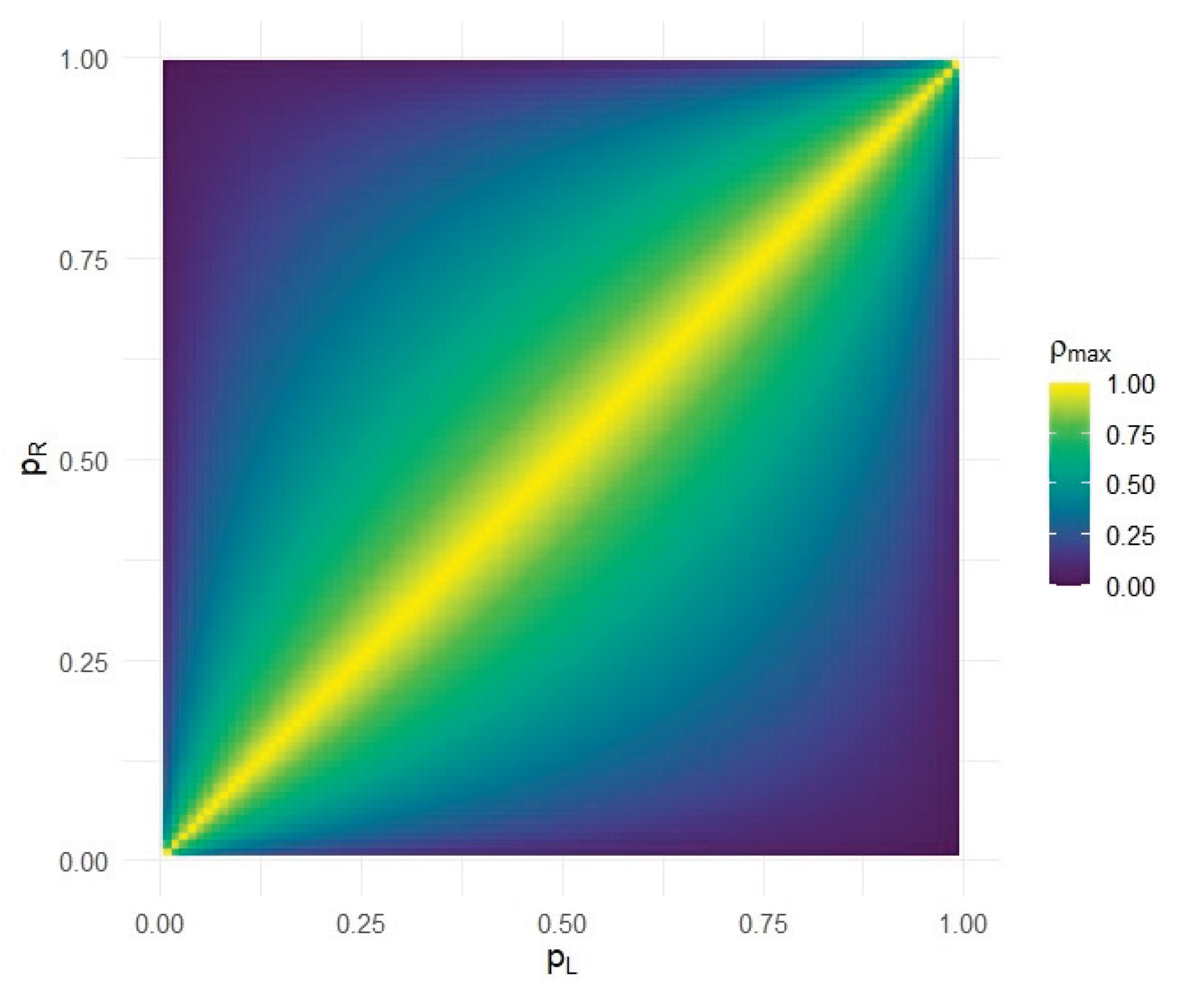
Figure 2. Bilateral prevalence as a function of within-subject dependence. Bilateral prevalence (

π_{B} = P r (Y_{L} = 1, Y_{R} = 1)

) as a function of the dependence parameter λ. Bilateral prevalence increases linearly from the independence value (

p_{L} p_{R}

) to the maximal feasible value (

m i n (p_{L}, p_{R})

). The dashed vertical line indicates the midway assumption (λ = 0.5). In contrast to laterality measures, bilateral prevalence remains stable and well behaved across the entire admissible dependence range.

Figure 2. Bilateral prevalence as a function of within-subject dependence. Bilateral prevalence (

π_{B} = P r (Y_{L} = 1, Y_{R} = 1)

) as a function of the dependence parameter λ. Bilateral prevalence increases linearly from the independence value (

p_{L} p_{R}

) to the maximal feasible value (

m i n (p_{L}, p_{R})

). The dashed vertical line indicates the midway assumption (λ = 0.5). In contrast to laterality measures, bilateral prevalence remains stable and well behaved across the entire admissible dependence range.

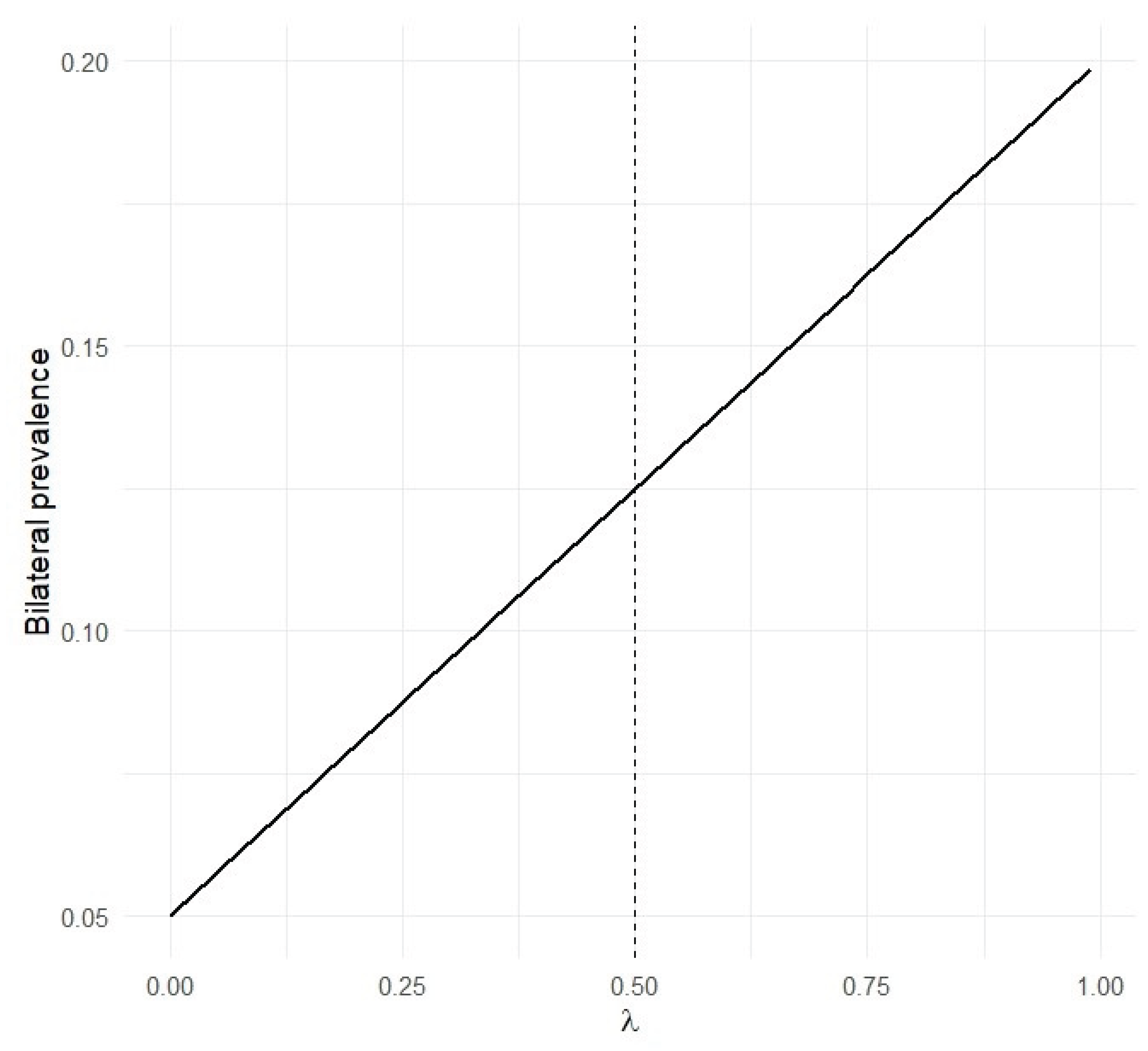
Figure 3. Paired log odds ratio as a function of within-subject dependence. Deterministic relationship between the paired log odds ratio for laterality and the dependence parameter λ, for fixed marginal prevalences. The curve is smooth and monotone but becomes increasingly steep as λ approaches 1, reflecting the boundary degeneracy of the paired odds ratio when one discordant component vanishes. The dashed vertical line marks the midway assumption (λ = 0.5), which lies well within the stable region.

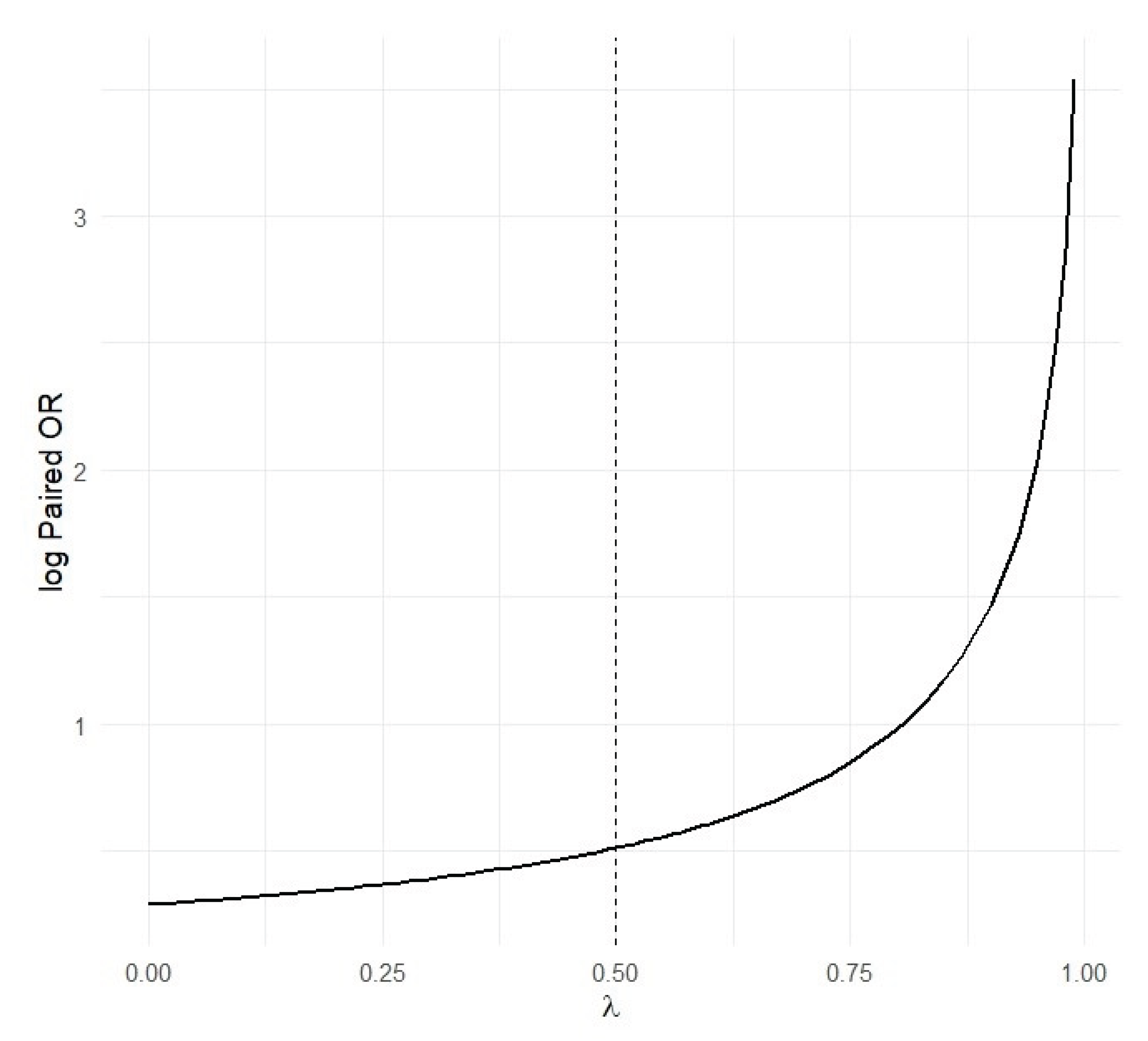
Figure 4. Monte Carlo behavior of the paired log odds ratio under increasing dependence. Monte Carlo mean (solid line) and 95% simulation envelope (shaded region) of the paired log odds ratio as a function of λ. Variability is limited for moderate dependence levels but increases sharply as λ approaches 1, even at moderate sample sizes. The dashed vertical line indicates the midway assumption (λ = 0.5), which is located in a region of low variability and numerical stability.

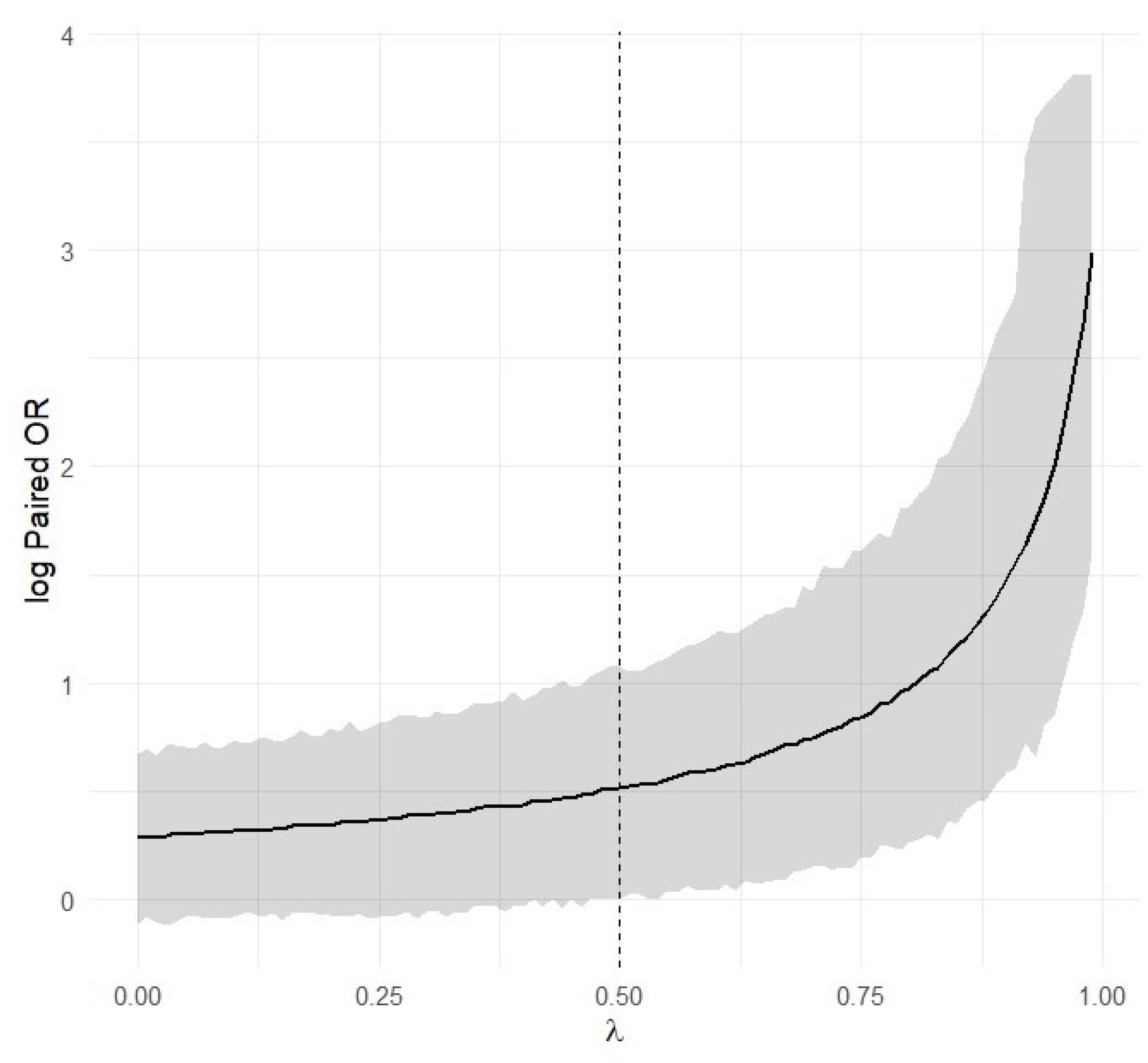
Figure 5. Expected standard error under uncertainty in dependence. Each curve represents the Monte Carlo estimate of

E [S E (\hat{δ}; λ)]

when the dependence parameter λ is treated as a random variable with fixed mean and increasing variance. Uncertainty is introduced on the logit scale, ensuring that λ remains within its admissible range. The horizontal axis reports the induced variance of λ on the probability scale, rather than the variance of the latent logit parameter. The near-linearity and shallow slope of the curves for small to moderate Var(λ) indicate that laterality inference is insensitive to moderate misspecification of the dependence assumption. Only when uncertainty becomes extreme does the expected standard error increase appreciably, reflecting propagation of dependence uncertainty into the paired odds ratio.

Figure 5. Expected standard error under uncertainty in dependence. Each curve represents the Monte Carlo estimate of

E [S E (\hat{δ}; λ)]

when the dependence parameter λ is treated as a random variable with fixed mean and increasing variance. Uncertainty is introduced on the logit scale, ensuring that λ remains within its admissible range. The horizontal axis reports the induced variance of λ on the probability scale, rather than the variance of the latent logit parameter. The near-linearity and shallow slope of the curves for small to moderate Var(λ) indicate that laterality inference is insensitive to moderate misspecification of the dependence assumption. Only when uncertainty becomes extreme does the expected standard error increase appreciably, reflecting propagation of dependence uncertainty into the paired odds ratio.

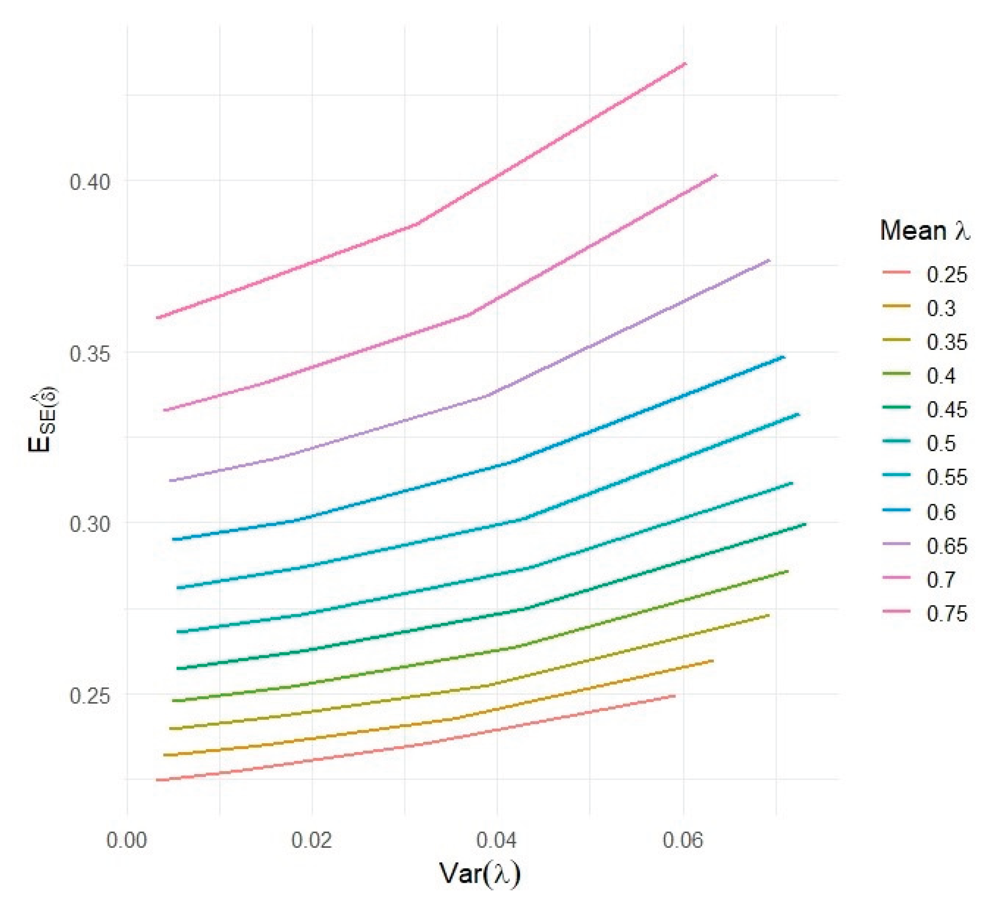
Figure 6. Implied midpoint correlation under unequal marginal prevalences. Correlation implied by the midway dependence assumption (

λ = 0.5

) plotted as a function of the marginal prevalence ratio

κ = p_{R} / p_{L}

, for several baseline values of

p_{L}

. The implied correlation is not constant and varies systematically with marginal asymmetry, emphasizing that correlation is not a transportable parameter in paired binary settings.

Figure 6. Implied midpoint correlation under unequal marginal prevalences. Correlation implied by the midway dependence assumption (

λ = 0.5

) plotted as a function of the marginal prevalence ratio

κ = p_{R} / p_{L}

, for several baseline values of

p_{L}

. The implied correlation is not constant and varies systematically with marginal asymmetry, emphasizing that correlation is not a transportable parameter in paired binary settings.

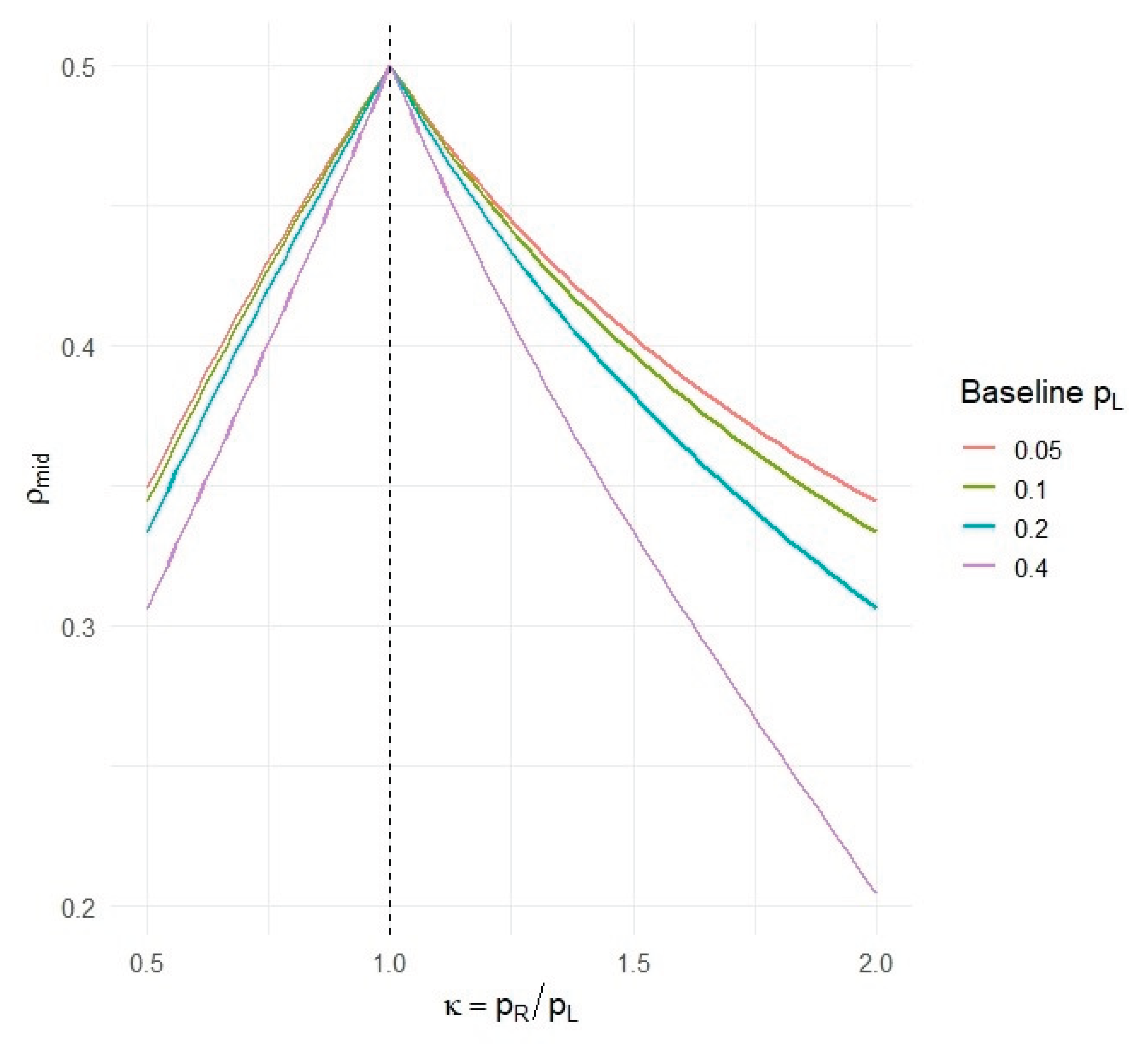
Figure 7. Precision impact of the midway dependence assumption under unequal marginals. Ratio of the standard error of the paired log odds ratio under the midway dependence assumption (

λ = 0.5

) to that under independence (

λ = 0

), plotted against

κ = p_{R} / p_{L}

for several baseline values of

p_{L}

. Values below 1 indicate improved precision under the midway assumption relative to independence; the magnitude of this effect depends on both the baseline prevalence and the degree of marginal asymmetry.

Figure 7. Precision impact of the midway dependence assumption under unequal marginals. Ratio of the standard error of the paired log odds ratio under the midway dependence assumption (

λ = 0.5

) to that under independence (

λ = 0

), plotted against

κ = p_{R} / p_{L}

for several baseline values of

p_{L}

. Values below 1 indicate improved precision under the midway assumption relative to independence; the magnitude of this effect depends on both the baseline prevalence and the degree of marginal asymmetry.

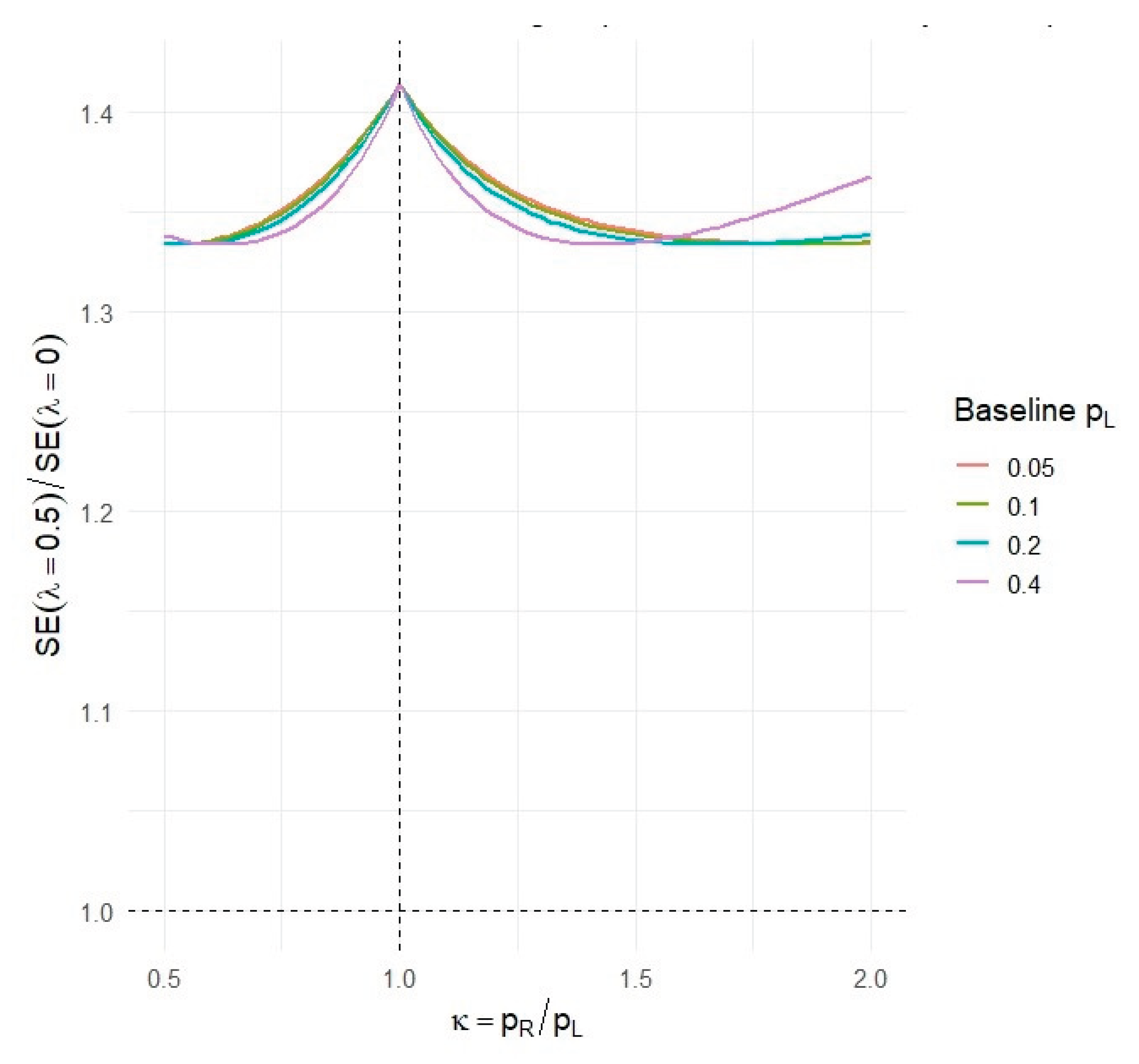
Figure 8. Maximum feasible phi for rare and imbalanced anatomic variants. Heatmap of the maximum feasible phi correlation,

ϕ_{m a x}

, as a function of left–right marginal imbalance

κ = p_{R} / p_{L}

and baseline left-side prevalence

p_{L}

(log scale), restricted to rare variants (

p_{L} \leq 0.10

). The feasible correlation range is determined by Fréchet bounds on the joint probability

p_{11}

. For rare variants, the lower feasible bound of

ϕ

approaches zero, rendering strong negative correlation infeasible, while the upper bound is governed primarily by marginal imbalance rather than rarity itself. Under the midway dependence hypothesis (

λ = 0.5

), which places

p_{11}

halfway between independence and maximal feasible concordance, the induced correlation satisfies

ϕ_{mid} \approx \frac{1}{2} ϕ_{m a x}

in the rare-variant regime, highlighting that the midpoint corresponds to a margin-dependent correlation scale rather than a fixed value.

Figure 8. Maximum feasible phi for rare and imbalanced anatomic variants. Heatmap of the maximum feasible phi correlation,

ϕ_{m a x}

, as a function of left–right marginal imbalance

κ = p_{R} / p_{L}

and baseline left-side prevalence

p_{L}

(log scale), restricted to rare variants (

p_{L} \leq 0.10

). The feasible correlation range is determined by Fréchet bounds on the joint probability

p_{11}

. For rare variants, the lower feasible bound of

ϕ

approaches zero, rendering strong negative correlation infeasible, while the upper bound is governed primarily by marginal imbalance rather than rarity itself. Under the midway dependence hypothesis (

λ = 0.5

), which places

p_{11}

halfway between independence and maximal feasible concordance, the induced correlation satisfies

ϕ_{mid} \approx \frac{1}{2} ϕ_{m a x}

in the rare-variant regime, highlighting that the midpoint corresponds to a margin-dependent correlation scale rather than a fixed value.

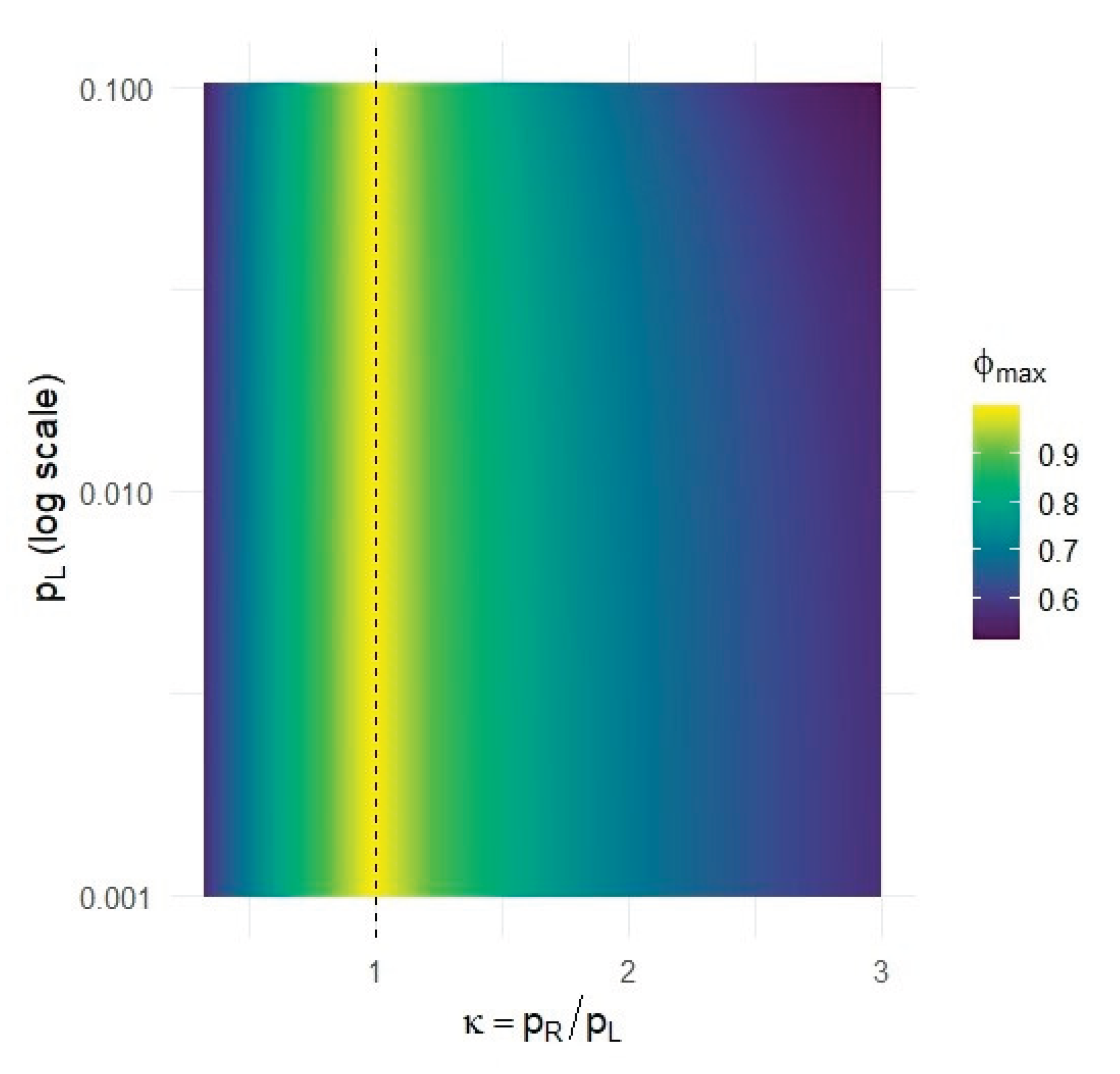
Figure 9. Invariance of the midway dependence hypothesis and margin-dependent expression of correlation under rare variants. The figure illustrates the relationship between the feasibility-based dependence index λ and the implied phi correlation (φ) as a function of left–right imbalance

κ = p_{R} / p_{L}

in the rare-variant regime (

p_{L}, p_{R} \leq 0.1

). The dashed horizontal line (right axis) represents the midway dependence hypothesis (

λ = 0.5

), which is fixed by definition. The solid black curve shows the maximum feasible phi correlation

ϕ_{m a x}

as constrained by the marginals, while the blue curve shows the correlation

ϕ_{mid}

implied by

λ = 0.5

. Under symmetry (

κ = 1

),

ϕ_{mid} \approx 0.5

, whereas increasing imbalance reduces the attainable correlation despite an unchanged λ. The right-hand axis is a linear rescaling used solely for visualization.

Figure 9. Invariance of the midway dependence hypothesis and margin-dependent expression of correlation under rare variants. The figure illustrates the relationship between the feasibility-based dependence index λ and the implied phi correlation (φ) as a function of left–right imbalance

κ = p_{R} / p_{L}

in the rare-variant regime (

p_{L}, p_{R} \leq 0.1

). The dashed horizontal line (right axis) represents the midway dependence hypothesis (

λ = 0.5

), which is fixed by definition. The solid black curve shows the maximum feasible phi correlation

ϕ_{m a x}

as constrained by the marginals, while the blue curve shows the correlation

ϕ_{mid}

implied by

λ = 0.5

. Under symmetry (

κ = 1

),

ϕ_{mid} \approx 0.5

, whereas increasing imbalance reduces the attainable correlation despite an unchanged λ. The right-hand axis is a linear rescaling used solely for visualization.

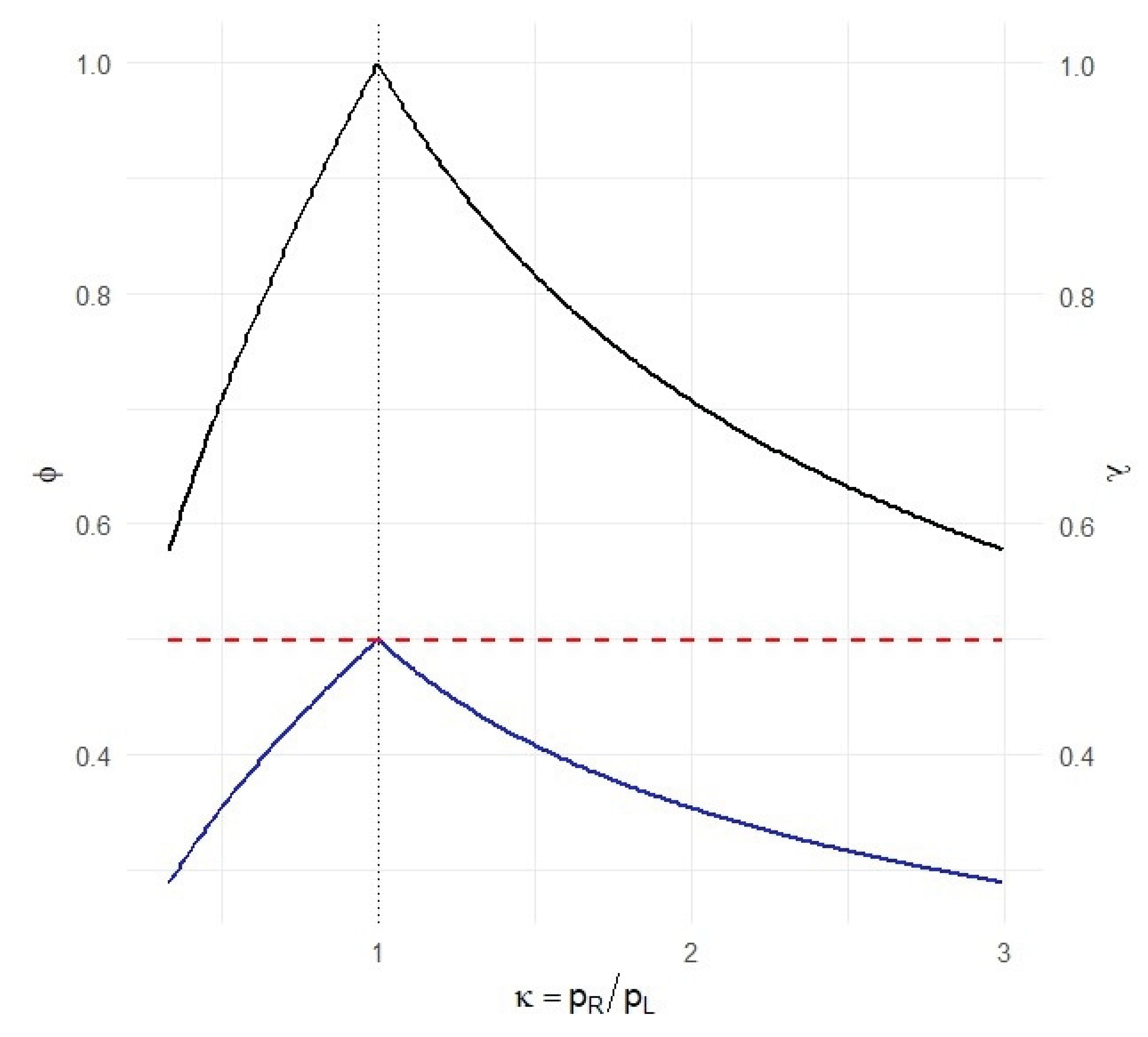
Table 1. Exact phi correlation implied by the midway dependence hypothesis for rare anatomic variants.

Maximum feasible phi –φ(max)
pL	k=0.333	k=0.5	k=1	k=2	k=3
0.001	0.577	0.707	1.000	0.707	0.577
0.005	0.576	0.706	0.998	0.705	0.576
0.010	0.575	0.705	0.995	0.704	0.575
0.050	0.565	0.695	0.950	0.685	0.565
0.100	0.548	0.674	0.900	0.660	0.548
Phi under midway hypothesis –φ(mid) = 0.5 ·φ(max)
pL	k=0.333	k=0.5	k=1	k=2	k=3
0.001	0.289	0.354	0.500	0.354	0.289
0.005	0.288	0.353	0.499	0.353	0.288
0.010	0.287	0.353	0.498	0.352	0.287
0.050	0.283	0.348	0.475	0.343	0.283
0.100	0.274	0.337	0.450	0.330	0.274

Table 2. How to meta-analyze laterality and bilateralism in anatomic variants.

Data reported in primary studies	Appropriate endpoint	Methodological approach	Dependence assumption needed?
Full paired table (left/right per individual)	Laterality	Paired odds ratio (discordant counts)	No
Full paired table	Bilateralism	Bilateral prevalence	No
Discordant counts only	Laterality	Paired odds ratio	No
Marginal left and right prevalences only	Laterality	Paired odds ratio reconstructed via dependence index	Yes
Marginal left and right prevalences only	Bilateralism	Bilateral prevalence via dependence index	Yes

Table 3. Summary of practical recommendations for the design, analysis, and reporting of meta-analyses of anatomic variants based on paired binary data.

Recommendation	Rationale
Distinguish clearly between outcomes	Treat laterality (right-only vs left-only manifestation) and bilateralism (presence on both sides) as distinct endpoints
Prefer paired measures for laterality	Use the paired odds ratio when individual-level pairing is conceptually present, even if incompletely reported
Report bilateral prevalence whenever possible	Bilateral prevalence is a stable and anatomically meaningful quantity that complements laterality
State dependence assumptions explicitly	When joint left–right data are unavailable, clearly report the assumed within-subject dependence model
Use feasibility-based sensitivity analysis	Evaluate robustness across the admissible dependence range (e.g., independence, midway, boundary)
Avoid variance-stabilizing transformations designed for independent data	Such transformations obscure pairing and complicate anatomical interpretation

Disclaimer/Publisher’s Note: The statements, opinions and data contained in all publications are solely those of the individual author(s) and contributor(s) and not of MDPI and/or the editor(s). MDPI and/or the editor(s) disclaim responsibility for any injury to people or property resulting from any ideas, methods, instructions or products referred to in the content.

© 2026 by the authors. Licensee MDPI, Basel, Switzerland. This article is an open access article distributed under the terms and conditions of the Creative Commons Attribution (CC BY) license (http://creativecommons.org/licenses/by/4.0/).

Meta-Analysis of Paired Binary Data with Unobserved Dependence: Insights from Laterality and Bilateralism in Anatomy

Abstract

Keywords:

Subject:

1. Introduction

1.1. Paired Observations and Why They Matter in Anatomy

1.2. The Unavoidable role of Dependence Assumptions

1.3. Laterality and Bilateralism as Complementary Outcomes

1.4. Existing Statistical Frameworks for Paired Binary Outcomes

1.5. A Feasibility-Based Approach to Unreported Dependence

1.6. Partial Pairing in Real-World Anatomical Datasets

1.7. Scope, Aims, and Structure of the Present Study

2. Materials and Methods

2.1. Paired Binary Data Structure and Notation

2.2. Target Estimands: Laterality and Bilateralism

2.2.1. Laterality

2.2.2. Bilateralism

2.3. Feasible Joint Distributions

2.4. Feasibility-Based Dependence Parameterization

2.5. The Midway Dependence Hypothesis

2.6. Derived Correlation Measures and Non-Invariance

2.7. Exact Feasible Range of the Phi Correlation

2.8. Behavior of the Midway Dependence Hypothesis Under Rare and Imbalanced Marginals

2.9. Dependence Parameterization Under Rare Variants

2.10. Simulation Study Design

2.11. Propagation of Uncertainty in the Dependence Assumption and Unequal Marginals

2.11. Computational Implementation and Software

3. Results

3.1. Why Not Just Fix the Amount of Correlation?

3.2. Theoretical Behavior of Bilateral Prevalence and Laterality

3.3. Monte-Carlo Behavior and Boundary Instability

3.4. Complementary Behavior of the Co-Primary Endpoints

3.5. Robustness to Uncertainty in the Dependence Assumption

3.6. Unequal Marginal Prevalences and the Behavior of the Midway Hypothesis

3.7. Rare Variants and Marginal Imbalance

4. Discussion

4.1. Laterality and Bilateralism as Complementary Endpoints

4.2. Boundary Degeneracy and Instability of Laterality

4.3. The midway Dependence Hypothesis as a Neutral Reference

4.4. Robustness Under Uncertainty and Marginal Imbalance

4.5. Relation to Classical Paired and McNemar-Type Analyses

4.6. Extensions: Sex-Relatedness and Alternative Dependence Models

4.7. Implications for Current Practice in Anatomic Meta-Analysis

4.8. Relation to Variance-Stabilizing Transformations

4.9. Strengths and Limitations

5. Conclusions

Supplementary Materials

Funding

Institutional Review Board Statement

Informed Consent Statement

Data Availability Statement

Acknowledgments

Conflicts of Interest

Abbreviations

Appendix A: Formal Properties of Feasibility-Based Dependence Parameterization

Appendix A.1. Setup: Paired Laterality Data

Appendix A.2. Feasibility, Variance Monotonicity, and Extremal Behavior

Appendix A.3. The midway dependence hypothesis

References

MDPI Initiatives

Important Links

Subscribe