
Submitted:
06 February 2026
Posted:
06 February 2026
You are already at the latest version
Abstract
Currently, research aimed at optimizing the power rating and energy capacity of electrical energy storage (EES) systems while accounting for multiple sources of uncertainty remains underrepresented in the scientific literature, due to the complexity of solving multidimensional uncertainty problems in microgrids. Regarding the comprehensive assessment of EES parameters considering the influence of various factors, despite numerous studies dedicated to the evaluation and rational selection of EES parameters, this task remains largely unresolved. This paper proposes a methodology for selecting EES parameters that accounts for the uncertainty of wind power plant (WPP) generation and electric vehicle charging station (EVCS) load, EES performance degradation, as well as the reliability and cost of microgrid implementation to ensure uninterrupted operation of EV supply equipment within a distribution network with limited available power capacity. The developed method and EVCS load profile model enable the generation of a time-based power profile under input data uncertainty. The work presents a mathematical model of microgrid operation that considers the integrated performance of EES, WPP, and EVCS. The EES parameter selection methodology is demonstrated using examples of various system configuration scenarios.
Keywords:
distribution networks
; electrical energy storage systems
; electric vehicle charging stations
; electric vehicles
; load profile model
; load profile uncertainty
; microgrid
1. Introduction
According to the International Energy Agency (IEA), the annual growth in global electricity demand is projected to be 3.9% from 2025 to 2027, marking the fastest growth rate in recent years [1]. Currently, it is becoming increasingly difficult for new consumers to connect to the power grid. Due to a sharp rise in demand for grid connection, enterprises face significant delays in connecting to existing overloaded networks, with wait times potentially reaching up to 8 years [2]. This hinders infrastructure development and constrains economic growth. As reported by the IEA, at least 1500 GW of global clean energy projects have been halted or delayed due to a lack of grid connection availability, necessitating approximately $700 billion in grid investments worldwide [3].
Global electric vehicle (EV) sales reached a record 17.1 million units in 2024, representing a 25% increase from the previous year [4]. This rapid growth in electric mobility necessitates further development of charging infrastructure. In 2023, the number of public charging points increased by approximately 40%. Notably, by the end of the year, fast chargers accounted for 35% of all public charging points, a growth rate surpassing that of slow chargers [5].
The demand for EV charging often coincides with the grid’s peak load hours, typically when a large number of EVs return home simultaneously. This, in turn, increases peak power demand, reduces reserve capacity, degrades power quality, and heightens the risk of network failures. This issue is particularly acute for low-voltage distribution networks (DNs).
Distribution networks are also experiencing a growing share of uncertain elements, such as generation from renewable energy sources (RES) and load from EVs. The uncertainty of load warrants separate investigation, as most existing research primarily focuses on uncertainties related to RES. Meanwhile, it is evident that electric vehicle charging station (EVCS) load is also stochastic, as EV charging behavior is uncertain and can vary depending on numerous parameters, including the number of vehicles charging, battery capacity, state of charge, and charging duration. Furthermore, the population of EVs in use is constantly changing, leading to fluctuations in overall charging demand and variations in load profiles. These uncertainties complicate accurate EV load forecasting and planning, necessitating the use of stochastic modeling methods to account for the inherent variability and unpredictability of EV load.
Current research predominantly focuses on optimal EVCS siting [6,7,8,9]. These studies mainly investigate the problem of selecting locations most convenient for EV users from the perspectives of spatial-geographical placement, logistics, and charging demand activity. Some works [10,11] examine the use of RES and electrical energy storage (EES) systems when integrating EVCS to reduce grid capacity charges. Research in [12,13] addresses the optimal siting of EVCS to improve reliability and reduce power losses in the distribution system. The consideration of uncertainties in charging demand, as well as RES, affecting optimal EVCS placement, has been explored in [10,14,15].
The number of studies that account for grid connection constraints for EVCS, including limited available power capacity, remains insufficient. This is particularly relevant for connecting high-power EVCS to existing DNs. The growing EVCS load on DNs is driving a shift toward alternative energy solutions. The creation of microgrids incorporating EES systems becomes a relevant approach to reduce dependency on the main grid and support EVCS operation.
Battery storage technologies, due to their instantaneous response and ability to stabilize grid parameters, are becoming a key tool for frequency regulation and maintaining power quality. Thanks to the flexible configuration of their power and energy capacity, EES systems can provide discharge over several hours, which helps optimize daily load profiles and prevent overloading of grid elements such as power lines or transformer substations. However, deploying high-energy-capacity EES in networks with limited power transfer capability requires reserve capacity for their charging during periods of low energy consumption. This process can be implemented using distributed generation, including RES.
Contemporary methods for sizing EES systems in microgrids or distribution networks face a number of challenges stemming from the intermittent nature of RES generation and loads, such as those from EVCS. These factors complicate the search for optimal storage parameters that consider not only their cost but also the dynamics of their lifespan reduction caused by irregular charge-discharge cycles.
Consequently, there is a need to develop a comprehensive approach for sizing EES systems and RES. Such an approach should be based on the mathematical modeling of a microgrid connected to the centralized grid and should ensure the coordinated operation of storage, RES, and consumers.
The aim of this work is to investigate the problem and develop a methodology for selecting parameters of EES systems in microgrids, considering the integration of EVCS.
The scientific novelty of the research lies in the development of a comprehensive methodology for selecting EES parameters under conditions of high uncertainty from both EVCS load and RES generation, while accounting for EES degradation, economic indicators, and network structural reliability metrics.
The practical significance is that the proposed methodology for sizing EES systems can be applied in distribution networks with limited power reserves, where synchronization of EVCS and RES is required to ensure deficit-free system operation
2. Electrical Energy Storage Sizing Methods
Modern research focuses on calculating the optimal energy capacity of EES systems under conditions of high uncertainty stemming from unpredictable RES generation and random load fluctuations. As RES output is intermittent, it introduces stochasticity into the power system’s balance. To compensate for such deviations, EES systems are employed; therefore, sizing EES requires analyzing the dynamics of RES generation and changes in energy consumption.
Optimal EES parameters are determined not only by their technical specifications but also by their degradation rate during operation. The degree of battery degradation directly depends on their functional role within the power system and on factors such as the share of renewables in the energy mix, charge-discharge cycle frequency, depth of discharge, and operating temperature.
Current research in this field aims to address two interconnected tasks: calculating EES energy capacity while accounting for degradation dynamics under specific network operating conditions, and developing control strategies that minimize the impact of aging factors—such as excessive depth of discharge, high cyclicity, extreme temperatures, or discharge current magnitude.
A key objective is to reduce the risk of energy undersupply to the grid. However, the actual service life of EES systems often deviates from manufacturer specifications due to differences in operational regimes [16]. This necessitates a holistic approach to EES design, where the balance between available energy capacity, energy efficiency, reliability, and longevity is defined by the specifics of their integration into the power system.
An analysis of publications on integrating EES into DNs and microgrids has identified key constraints affecting their parameter selection. In most studies, sizing the EES capacity is data-driven, yet the approaches often overlook the need for multi-factorial analysis. For instance, some research focuses solely on optimizing power flows, neglecting the interrelation between EES parameters, operational risks, and economic criteria. Therefore, the analysis of existing studies will also be conducted based on the criterion of selecting EES characteristics that enable a comprehensive solution assessment.
A wide range of optimization approaches is applied when designing power systems with integrated EES and RES. Among mathematical methods, mixed-integer linear programming (MILP) is prominent [17], while heuristic algorithms—such as the Firefly Algorithm [18] and Genetic Algorithms [19]—are actively used for solving nonlinear problems.
Given the instability of RES generation and load variability, selecting EES parameters requires specialized methods. These include stochastic optimization, encompassing Markov decision processes and scenario-based stochastic programming (SP) models; probabilistic approaches, such as chance-constrained programming [20,21] and analysis based on Markov chains [22]; and simulation methods, e.g., Monte Carlo simulation for uncertainty assessment [23,24,25].
Study [26] examines the optimal placement of EES to reduce power losses. The authors formulate the problem as a nonlinear integer optimization model, where EES placement and capacity parameters are discrete. However, the work lacks a comprehensive analysis of storage parameter selection considering other criteria that influence their design.
In another study [27], EES parameters are determined while accounting for their degradation. Despite this, the proposed model assumes an annual increase in energy capacity without evaluating the economic feasibility of such investments, the impact of additional capacity on system performance, or the long-term mitigation of storage degradation rates. Furthermore, both studies fail to consider the uncertainty caused by load fluctuations and RES generation instability, which is critical for optimal EES sizing.
Research [28] presents a comprehensive approach to optimizing the operating parameters of lithium-ion battery storage (rated energy capacity, depth of discharge, charge-discharge current, state-of-charge level) in DC microgrids. The primary goal is to reduce the operating costs of the EES system. The authors applied the rainflow counting method to analyze EES duty cycles; however, the model was limited to simplified charge-discharge scenarios without considering the impact of irregular cycles on battery degradation rates or the influence of RES generation stochasticity on storage sizing. Thus, the proposed methodology does not cover key factors associated with real-world operating conditions, reducing its practical applicability.
In study [29], EES is used to ensure the autonomous operation of a power system entirely dependent on RES during emergencies—such as damage to main power lines or scheduled maintenance. The simulation duration in such a system is determined by the recovery time of the damaged infrastructure. The authors propose a methodology for sizing the EES system that considers reliability requirements and a two-level control strategy for isolated grids where energy consumption is solely covered by wind generation. It is assumed that the optimal capacity of a sodium-sulfur (NaS) battery is achieved while maintaining a specified level of power supply continuity. However, the work lacks an analysis of the impact of wind power plant (WPP) output instability on EES sizing, as well as an assessment of storage degradation and lifespan when co-deployed with WPPs.
The main complexity in designing EES lies in calculating their optimal energy capacity under conditions of high uncertainty, caused by the irregular output of RES and the increasing integration of EVCS, which has a stochastic charging demand from EVs. Modern scientific research [20,21,23,30] examines methods for analyzing the impact of uncertainties on selecting EES characteristics.
Study [20] proposes a method for calculating EES parameters for microgrids with a high penetration of RES. To model uncertainties related to RES generation and load, the authors transformed them into chance constraints. Bernstein approximation was used as a mathematical tool to convert stochastic conditions into deterministic convex counterparts. It was assumed that load and RES generation fluctuations follow a normal (Gaussian) distribution, resulting in an approximated constraint on randomness.
Research [21] presents an approach to designing isolated microgrids that integrates the optimization of EES energy capacity with an operational strategy for battery-based storage. The primary goal of the method is to minimize the system’s total costs while preserving its reliability. To achieve this, the authors employ chance-constrained programming, which accounts for stochastic factors (load and generation uncertainty) and ensures that critical conditions are met with a specified probability. Particular attention is paid to constraints imposed on the battery state of charge. This prevents sizing the EES for highly improbable extreme scenarios, thereby reducing the risk of unjustified financial investment.
Work [30] presents a model for multi-period stochastic optimization for the dynamic control of batteries in DNs. The model aims to minimize the operating costs of a microgrid while considering the non-convex cost function associated with EES degradation. The authors employ a machine learning method—reinforcement learning, augmented with Monte Carlo tree search and knowledge-based rules. Due to the stochastic nature of distributed generation and EVCS load, the dynamic dispatch of EES is essentially a multi-period stochastic optimization problem (MSOP). The paper notes that one method for solving MSOPs is the application of Scenario-Based SP.
In most scientific works, the primary task when assessing EES parameters is to reduce total costs—both capital and operational. System reliability is treated as a constraint ensuring compliance with specified standards. For its quantitative assessment, standard metrics are used: Loss of Load Probability (LOLP) [20]; Loss of Load Expectation (LOLE) [17]; Loss of Power Supply Probability (LPSP) [18]; and Expected Energy Not Supplied (EENS) [29].
Thus, modern research lacks a methodology that comprehensively addresses the task of selecting EES parameters in microgrid networks. Such an approach should account for the influence of uncertainties (RES generation, load fluctuations), minimize their negative consequences, and integrate reliability criteria, storage degradation, and network upgrade costs.
3. Electrical Energy Storage Sizing Methodology for Microgrids
3.1. Problem Statement for Sizing EES to Supply EVCSs
The object of this study is a microgrid connected to a DN, with integrated operation of an EVCS, EES systems, and RES. In this research, WPPs are considered as the RES, as their intermittent generation, dependent on weather conditions, intensifies uncertainty within the power system. This results in frequent EES charge-discharge cycles, which accelerate their degradation and reduce their service life.
Considering the limitations of existing approaches to sizing EES systems, the following requirements are set for the developed methodology:
- ○
- The methodology must ensure adherence to power balance constraints and analyze energy deficit and surplus within the microgrid connected to the main grid, considering specified operational limits.
- ○
- The methodology must incorporate an assessment of the uncertainty associated with both EV supply equipment (EVSE) load and WPP generation.
- ○
- The methodology must model storage degradation under various operating regimes, accounting for the non-linear nature of degradation and random charge-discharge cycles.
- ○
- The methodology must include economic indicators and metrics of the network’s structural reliability.
These requirements are aimed at creating a comprehensive methodology for selecting EES parameters. Implementing the proposed approach necessitates the construction of several models that together form the overall EES sizing methodology. The structure and interrelation of these models are presented in Figure 1.
Blocks 1–5 represent the objects of the microgrid (MG) system under study: the external power system, consumers, the EES, the WPP, and other components (Blocks 2–5). The next level (Blocks 6–8) includes models for evaluating the parameters of these system objects. Input data for the simulation are fed from Blocks 2–5 into Blocks 6–7.
Block 4 defines the initial data regarding the power rating and energy capacity of the EES. These parameters are varied, taking into account the constraints from the balance equation (Block 7) and the co-optimization of EES and WPP parameters (Block 8). Data from Blocks 3 and 5, fed into Block 6, are processed to account for the uncertainty in net power balance changes during the EES parameter assessment.
The simulation results enable the solution of various sub-problems: assessing MG network reliability (Block 10), evaluating MG network cost (Block 11), and estimating EES degradation (Block 12). This facilitates the selection and updating of the MG network component parameters (Block 9).
A generalized algorithm for implementing the EES parameter selection model is presented in Figure 2. The following scenarios are considered when connecting additional load in the form of an EVCS to the DN:
a) If the existing DN can cover the demand of the connecting EVCS load and convergence is achieved, then DN expansion (by adding EES and WPP) is not required.
b) Otherwise, the DN is expanded by connecting an EES system, followed by an assessment of its parameters. Using an iterative method, the energy capacity of the EES is increased until convergence is achieved.
c) If a further increase in energy capacity does not lead to a reduction in the load deficit, this indicates that during off-peak load times (when the EES is in charging mode), there is insufficient available power from the grid to charge the EES. To maintain the EES at its nominal power and capacity, connecting additional sources of electrical energy, such as a WPP, is required. Thus, a WPP is installed on the EES side to support its charging, and on the EVCS side, the EES parameters are re-selected considering the integrated WPP.
3.2. Modeling of EVCS Electricity Consumption Profile Considering Uncertainty
The uncertainty of load warrants separate investigation, as most existing research focuses primarily on uncertainties related to RES. At the same time, it is evident that EVCS load is also stochastic, as EV charging behavior is uncertain and can vary depending on various parameters, such as the number of vehicles charging, battery capacity and state of charge, as well as charging duration. Furthermore, the population of EVs in use is constantly changing, leading to fluctuations in overall charging demand and variations in load profiles. These uncertainties complicate accurate forecasting and planning of EV load, necessitating the use of stochastic modeling methods to account for the inherent variability and uncertainty of EV load.
In this paper, the uncertainty of the EVSE load profile is assessed using a parametric model for probabilistic simulation employing the Monte Carlo method. The methodology involves generating load uncertainties using probability distribution functions.
To test the method, let us consider a scenario where it is necessary to determine the number of EVCSs so that each EV can connect without waiting. It is also required to obtain an aggregate electricity consumption profile to assess the feasibility of integrating such a load into the existing power grid.
Analyzing data on the number of EVs, we established that charging is required for 1000 vehicles over a week, with an average power demand per EV of 25 kW. Charging will be provided at a single location, i.e., one EVCS. In our case, the EVCS is located on a busy highway near a major metropolis. For these conditions, it is necessary to calculate the power consumption of the EVCS and the required number of charging points.
In this work, the Monte Carlo method is used to generate a load profile based on several random variables and to calculate output parameters in order to account for EVCS load uncertainty. These variables include: the charging start time for an EV (); the
Figure 3.
The algorithm for simulating the load profile of EVCS.
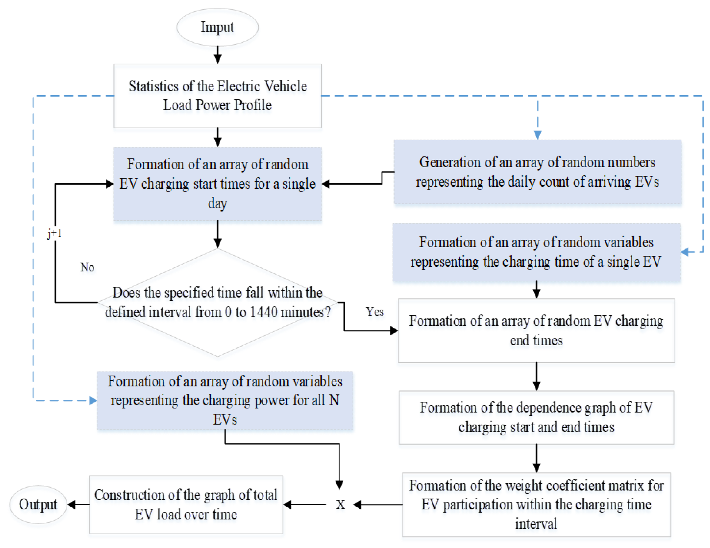
The model is initialized with the following input data: the simulation start time () and the total number of vehicles within the simulation interval (). Random load components, such as the charging start time and the power consumed by a single EV, are generated using probability distribution functions with corresponding parameters for the random variables.
Subsequently, an array of random integers is generated, representing the number of vehicles arriving for charging each day (). The daily number of vehicles follows a normal distribution, with the variance being a modifiable parameter. The number of vehicles on the final day of the simulation is adjusted so that the cumulative total matches the predefined parameter .
To analyze the diurnal EV consumption pattern, it is necessary to examine data on charging start times over a specific interval, such as one month. Accordingly, statistical data on the quantity and connection intensity of EVs are used to analyze the daily load profile. Based on these data, an empirical daily charging profile is constructed through mathematical processing and averaging of the statistical data (Figure 4 and Figure 5). The EV load profile can be characterized by several load peaks, such as evening, night, or morning consumption maxima. Based on the obtained statistics, weekdays typically exhibit distinct evening and nighttime load peaks.
For the mathematical description of generating a random daily profile based on the historical data of an EVSE station, let us represent the one-dimensional time series of EVCS power as follows:
where is the total number of measurement points; is the power value at time , the sampling interval is 10 min (i.e., 144 points per day).
Let us determine the number of complete days:
The data is transformed into a matrix, which enables the calculation of interval-specific statistics (e.g., mean and standard deviation) for each time of day:
Next, we calculate the average EVCS load profile. The mean power value for each time slot is calculated as:
We generate a synthetic daily profile. For each time slot, Gaussian noise is added to the mean value. The noise is normalized: , and its amplitude is controlled by parameter .
where is the mean power value at time ; is the standard deviation at time ; is normally distributed noise; is a scaling coefficient (noise level).
Figure 6 presents the average daily profile and a randomly generated day, demonstrating how well the random day reflects the underlying average trend.
Figure 7 shows an actual daily profile and a randomly generated profile, demonstrating the correspondence between the synthetic day and the real-world observation.
Figure 8 presents a comparison of averaged profiles, demonstrating the stability of the simulation results under averaging.
The array of charging end times is generated randomly using a normal distribution. The charging start time is added to the mathematical expectation () of the charging duration () and a random positive or negative increment of this time with a standard deviation () equal to one-third of the desired variation interval:
where is the charging end time; is the charging start time; is the expected value (mean) of the charging duration (); is a random time increment, normally distributed with zero mean and standard deviation .
Similarly, random power load values are generated for all EVs. Next, a weight coefficient matrix is created to determine the contribution of the -th EV to the overall load profile. Matrix of dimension rows by columns is formed, where represents the simulation time step.
Each time step () from the first to the last is iterated sequentially for each -th EV. If the current time falls within the charging interval for the -th vehicle (i.e., the current time is greater than its start time and less than its end time), then the corresponding matrix element is set to 1; otherwise, it is set to 0. This procedure is repeated for all EVs:
where is a binary variable (1 if the EV is within the load profile time interval); is a matrix of dimensions ; is the number of time steps in the simulation interval; is the total number of EVs.
To form the aggregate load profile, the sum of the product of the weight coefficient matrix and the power of each EV is calculated:
where is a matrix of dimensions ; is the vector of EV load powers.
To illustrate the load profile modeling example, we define the initial parameters: simulation interval duration — 7 days, number of vehicles in the simulation interval — 1000 units. We assume that the expected value (mean) of the EV charging time follows a normal distribution, where the parameters of the random variable are: h and triple standard deviation h. This parameter can conventionally be considered the range of probable charging time variation according to the “three-sigma rule”. Simulation time step — one minute.
The input parameters can vary depending on the research objectives. The simulation interval can be a day, a week, or a month. The choice of a minute time step for modeling the EVCS load profile is due to the high load dynamics, as a minute step allows tracking these changes. Furthermore, for accurate modeling of charging processes, which can last from several tens of minutes to several hours, a minute step provides a more detailed representation of the charging process. It also allows for accounting short-term processes, primarily associated with fast EVCSs.
To make the study relevant for Russia, the normal distribution is chosen so that the mean value of the expected power parameter per EV is close to the average power of the most popular EV models. Therefore, it is assumed that the parameters of the random variable are kW and kW, and the powers of arriving vehicles are randomly selected from this distribution. Subsequently, an array of random integers is generated, corresponding to the number of vehicles arriving for charging each day. The quantity follows a normal distribution.
Next, an array of random charging start times is generated using the algorithm presented earlier. Then, an array of charging end times is formed. The graph of charging start and end times versus the sequential number of the EV is shown in Figure 9. After this, the aggregate load profile of EVs for the entire period is formed, which is shown in Figure 10.
Below is the daily load profile for one of the first simulation days with a one-minute time step (Figure 11).
Figure 12 shows the number of EV connections over time, obtained from the simulation results. The graph indicates that for this variation of the random variable distributions, the maximum daily total number of simultaneously charging vehicles ranges from 40 to 55, given the specified total number of connecting vehicles — 1000 units over a week.
Thus, the distinctive feature of the proposed EVCS load profile modeling approach is its ability to comprehensively account for all key factors and parameters through a unified model that ensures their interconnection. This method allows the use of a different set of values, drawn from probability distributions, with each simulation run, thereby covering a wide spectrum of possible scenarios. The simulation accounts for the temporal intensity of EV connections, enabling further analysis of the load profile for solving the problem of selecting EES system parameters to power EVCS.
3.2. Modeling of WPP Electricity Generation Profile
Since WPP generation introduces uncertainty into the evaluation of EES parameters, it is necessary to account for the stochastic nature of WPP electricity output. The modeling of random WPP operation (power output) is based on statistical data reflecting the trend of WPP power generation. An empirical probability distribution law for wind speed was formulated using available discrete data.
The analysis revealed that while the generated wind speed profiles have similar integral characteristics to the original dataset (probability density distribution), they fail to account for its temporal variation patterns. For instance, wind speed exhibits certain slow-changing trends, typically preventing sharp fluctuations over time. The generated data did not incorporate this inherent feature.
A mathematical framework was selected to replicate wind speed with analogous integral characteristics. It is proposed to use a model based on Markov chains, which is suitable for incorporating the probabilistic characteristics of the empirical distribution and models dependencies between consecutive values to preserve the inertia of wind speed changes. For this purpose, a matrix of transition probabilities (probabilities of how often one wind speed value follows another) was constructed, new data were generated using this transition matrix, and the smoothness of wind speed changes was ensured by limiting possible transitions. The algorithm is presented in Figure 13.
3.3. Mathematical Model of the Microgrid Network
To model the operation of a microgrid with EES, MILP is employed. Its use is driven by the need to combine discrete variables (e.g., selection of EES operating mode: charge/discharge) and continuous variables (state of charge, generation power level). Since load and generation vary over time, the problem is formulated as a multi-period one. In this study, a weekly planning horizon with an hourly time step is chosen, allowing for a detailed analysis of system dynamics.
To implement the MILP model, various constraints are imposed, including power balance and supply source capacity limits, constraints on WPP operation, and constraints on the EES operating mode. For a more efficient solution, all subsequent constraints are formulated within a mixed-integer linear framework for each time interval and for each scenario of uncertain elements:
where is total power demand of the network and the EVCS at time t, is power supplied from the grid, is available energy capacity of the EES, is WPP power output, is power deficit, i – scenario index for data samples.
Given the constraint of available DN capacity:
where is the minimum permissible network transfer capacity.
The scheduled output power of the WPP is constrained by its minimum and maximum output limits:
where are the minimum and maximum output powers of the WPP, respectively.
EES Constraints. The battery state of charge must be constrained within a specified range:
where is the nominal energy capacity, and is the corresponding state of charge at the initial time, ensuring that the state of charge at any time is constrained within the considered range.
The output power of the EES satisfies the following conditions:
where is the output power (positive values indicate discharge, negative values indicate charge); Pchb is the upper limit for charging power; Pdisb is the upper limit for discharging power.
Given that the simulation spans one week, the assessment includes not only the power but also the energy capacity of the EES. Energy capacity is defined as the product of the EES discharge time and its power. Formula (15) describes the relationship between the nominal power and the nominal energy capacity of the EES:
where is the energy capacity of the EES, and is the discharge time of the EES.
The output energy capacity of the EES satisfies the following conditions:
where and are the lower and upper limits of energy capacity, respectively.
The charge-discharge algorithm of the EES system is determined considering the compensation of the energy deficit occurring during peak hours. If the EES energy capacity is greater than zero during an energy deficit, the EES discharges (17). If the current (available) EES energy capacity is less than its maximum energy capacity, then the charging mode is activated, where the charging power corresponds to equation (18). The EES charges provided there is available power from the grid and RES. When the balance condition is met or there is an energy surplus, the EES remains in standby mode (19).
3.4. Multi-Criteria Analysis Method
The method for multi-criteria analysis of EES parameter selection is based on the quantitative assessment of criteria and the determination of their geometric sum, which comprises three indicators: the cost of distribution network expansion planning (), the degree of EES degradation (), and the microgrid SAIDI reliability (). To construct the diagram presented in Figure 14, all criteria are converted into relative units. In this case, the criteria form a scalene triangle with coordinates (20)–(22).
The optimal option is selected based on the minimal triangle area, which is determined by the expression:
3.5. Methods for Assessing Criteria for EES Parameter Selection
For assessing degradation, a semi-empirical model presented in work [31] was used as the basis. This model can be utilized for predicting the service life of EES systems when solving various tasks in distribution network operation, including scenarios with uneven load and generation from WPPs, where the EES follows a stochastic charge and discharge signal. The model is also applicable to lithium-ion battery packs. Semi-empirical models do not require extensive statistical data, unlike physical degradation models or machine learning-based models. Nevertheless, these models demonstrate relatively high prediction accuracy, though their results are limited by the dataset used. To evaluate EES degradation, a data-driven semi-empirical model for Lithium Nickel Manganese Cobalt Oxide (NMC) batteries is employed. This model estimates the loss of battery cell lifetime based on operational state-of-charge profiles.
Within the model, the Rainflow counting algorithm is applied to the current state-of-charge profile of the EES to count incomplete cycles. This algorithm is suitable for assessing irregular EES charge-discharge cycles.
A combined model of calendar and cyclic aging is then used. These are linear degradation processes relative to the number of cycles:
where is linearized degradation model, is linearized degradation model for calendar aging, is time period, is average state of charge, is average cell temperature, is linearized degradation model for cyclic aging, is number of cycles identified in the operation, is cycle index, is indicator of a full or partial cycle.
Since the degradation process is nonlinear, being accelerated at the beginning and end of the service life, a model describing the growth mechanism of the Solid Electrolyte Interphase (SEI) layer is used to capture the nonlinear nature of degradation. Thus, the equation takes the form (25-26), where equation (25) – the SEI model – is applied to cyclic test data, and equation (26) is applied to calendar aging data. Approximation algorithms are used to fit the values , , and in equations (25-26) to experimental degradation data.
To account for distribution network reliability constraints, the reliability assessment metric PSAIDI is used, as per formula (27). This index is defined by the average duration of equipment downtime due to technical faults:
where: –the duration of the j-th interruption of electricity supply to consumers due to a technical fault, in hours, – the number of delivery points (nodes) affected by the j-th interruption of electricity supply due to a technical fault, in units, – the maximum annual number of delivery points (nodes), in units per year.
To estimate the cost of expanding the distribution network for creating a microgrid, it is assumed that all costs for installing individual system components are summed, as per formula (28). For a more accurate cost calculation, it is necessary to account for the specific parameters of each system component, as well as regional specifics.
where: is the total cost of distribution network expansion, is the cost of installing the EES system, is the cost of installing the WPP, represents other costs associated with system expansion (e.g., connection, design, installation costs, etc.).
4. Testing the Methodology
The methodology was tested by examining the feasibility of connecting an EVCS, using as an example its integration into the grid at an existing fueling station on the Volgograd-Astrakhan highway, Russia. It was necessary to forecast the EVCS load profile. For this purpose, the total number of vehicles arriving over a week was set to 1000 vehicles. Based on an empirical daily connection intensity profile and the parameters of random variables, the EVCS load profile was modeled. As a result, the maximum EVCS peak load reached 1.4 MW. When superimposing the EVCS electricity consumption profile onto the existing load profile of the fueling station, the combined maximum peak load increased to 1.8 MW (Figure 15). Consequently, the existing network — a 10 kV line with a limited 630 kVA transformer substation — cannot fully meet the additional connected load. It is necessary to consider several options for powering the EVCS.
Additionally, to analyze EVCS load uncertainty, a method using quantile analysis was considered (Figure 16). This allows for understanding the probability that the load will exceed a certain value, which can be critical for the design and operation of EVCSs and for sizing EES to compensate for energy deficits. In this work, the 50th quantile (median) was used for further research. This enables a more accurate assessment of the EES system characteristics required to ensure reliable operation under most scenarios.
For all scenarios, five base options with different network capacity parameters were modeled. Options 1 and 2: Transformers operate at 40% overload during peak hours. Option 4: Normal operation without changing the network’s capacity. Option 5: A twofold increase in network capacity due to reconstruction. Option 3: A combination of a twofold increase in network capacity and transformer operation at 40% overload. In Option 2, peak load reduction through limiting EVCS power during EV charging was additionally analyzed. To assess the impact of EES degradation and other criteria, Options 6–15 were also considered, which involve changes in EES energy capacity and the penetration share of WPP relative to the base parameters of Options 1–5.
Based on the proposed approach (Figure 1) and its implementation using MILP with constraints (10)–(19), EES parameters were evaluated for all options. Initial values were chosen according to the condition of fully covering the energy deficit (Equations 10–12). The results of the EES and WPP parameter assessment are presented in Table 1.
1.1. Comparison of Options
At the next stage, a quantitative assessment of the key criteria was performed: storage degradation, reliability, and the implementation cost of the microgrid network. The EES degradation for each of the scenarios is presented in Figure 17. The maximum degree of degradation is observed in Option 5 with a twofold increase in network capacity. This is explained by the increased charge-discharge cycles caused by the higher load on the EES to compensate for the power imbalance. The lowest degree of degradation was recorded in Option 10, characterized by an increase in EES energy capacity and a reduction in the installed capacity of the WPP. The reliability and cost characteristics of the microgrid network were also calculated. The reliability assessment results are presented in Figure 18.
Next, we will compare these Options using multi-criteria analysis based on the triangle area method. According to the obtained criteria, a diagram for selecting EES parameters is constructed (Figure 19)
For a more convenient analysis of the obtained options, let us rank the data according to three scenarios:
The first scenario assumes no possibility of connecting additional power from the grid, and the network is designed to operate under normal conditions throughout the entire period. The second scenario implies system operation at a 40% overload during peak load periods. The third scenario considers the possibility of connecting additional power from the grid through its reconstruction, and within this scenario, an option where the grid operates under overload (Option 3) is analyzed.
The analysis showed that the options of the first scenario are the most effective. Despite the high degree of EES degradation (27.07% and 29.57%), they allow for a significant reduction in costs due to less implementation of energy-intensive solutions. However, in some cases, connecting the EVCS may be unjustifiably expensive, or the technical conditions for connection may be absent. In this case, either Option 2 of the second scenario or Option 11 of the first scenario is considered.
Option 2 envisages a reduction in available power to lower the peak load and, consequently, reduce the required EES energy capacity. For example, if an arriving EV is charging, it will charge more slowly because we limit the power supplied by the grid, but consumption does not exceed the set limits.
Peak load reduction amounts to 2.79 MWh (9.78%) per week, but capital costs are reduced by only 0.08% compared to Option 1, and degradation changes insignificantly. Thus, for this scenario, Option 1 remains optimal.
For the first scenario, Option 11, which assumes a 9.78% reduction in peak load relative to Option 4, demonstrates the smallest area among the options. However, this change has an insignificant impact on all three criteria. Consequently, Option 4 has the smallest area in the third scenario.
Figure 20.
Comparison of Options Across Three Scenarios.
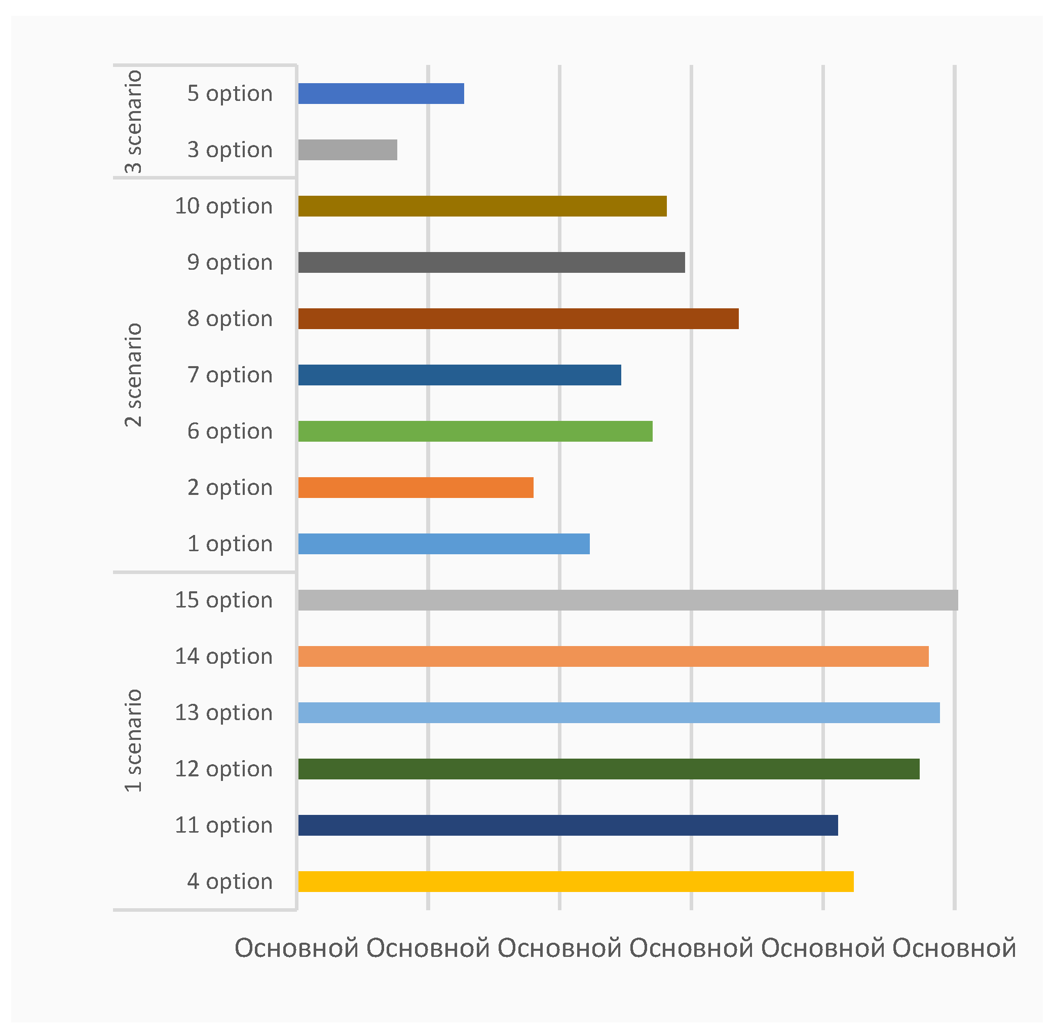
The results highlight the importance of selecting EES parameters that ensure an optimal balance between cost, degradation, and reliability. Options 3 and 5 are preferable when partially overcoming grid constraints, while Options 1 and 4 are relevant when it is impossible to increase network capacity.
5. Conclusion
The article presents a methodology for selecting parameters of EES systems in microgrids with integration of EVCSs. The model integrates a numerical method for simulating the EVCS load profile under uncertainty, microgrid network modeling, and the selection of EES parameters based on a multi-criteria analysis method. The quantitative assessment of parameter selection criteria includes modeling EES degradation, evaluating structural reliability, and calculating the cost of creating the microgrid network.
The article processed experimental data on the number of connecting EVs, based on which an averaged daily EVCS load profile was obtained. A combined probability distribution law was applied, corresponding to the empirical data and reflecting the intensity of EV connections. A parametric model was developed for generating the temporal EVCS load profile, accounting for key load uncertainty factors: charging start times, EV power consumption, charging duration, and the number of EVs. The practical significance of EVCS load modeling lies in the fact that a universal model will consolidate EV loads into a unified profile of randomly varying power with independent random variable parameters derived from processed experimental data.
The operation of the microgrid network in conjunction with the WPP, EES, and EVCS is described using MILP. This approach allows for formalizing EES charge-discharge processes based on the dynamics of electricity generation and consumption, as well as for evaluating EES and WPP parameters while considering power balance constraints.
Author Contributions
Conceptualization, I.S., H.B., N.S., K.P., I.I., D.F. and K.S.; methodology, N.S., D.F., I.B. and E.V.; software, N.S., and D.F..; validation, H.B., I.S.,, K.S., K.P., I.B.; formal analysis, I.S., D.F., I.I., N.S., D.F., and K.S.; investigation, N.S., A.K., I.S., and K.S.; resources, K.S.; data curation, D.F., A.K. N.S., K.P.; writing—original draft preparation, H.B., A.K. I.S., K.P., I.I., D.F. and K.S.; writing—review and editing, H.B., K.P., N.S., I.B., I.I., D.F. and K.S. visualization, N.S., K.P., D.F.; supervision, I.S., N.S., K.S. and I.I.; project administration, K.S., I.B., I.I., and D.F.; funding acquisition, K.S., I.I., I.B. and H.B. All authors have read and agreed to the published version of the manuscript.
Funding
This study is financed by the European Union-NextGenerationEU, through the National Recovery and Resilience Plan of the Republic of Bulgaria, project № BG-RRP-2.013-0001-C01.
Data Availability Statement
The original contributions presented in this study are included in the article. Further inquiries can be directed to the corresponding authors.
Conflicts of Interest
The funders had no role in the design of the study; in the collection, analyses, or interpretation of data; in the writing of the manuscript, or in the decision to publish the results.
References
- Demand, International Energy Agency, Available at: https://www.iea.org/reports/electricity-2025/demand.
- Europe’s battle for power spurs evolution of a new ecosystem for energy-hungry firms, CNBC Available at: https://www.cnbc.com/2025/03/05/europe-battle-for-power-heats-up-as-global-electricity-demand-accelerates.html.
- The clean energy economy demands massive integration investments now, International Energy Agency, Available at: https://www.iea.org/commentaries/the-clean-energy-economy-demands-massive-integration-investments-now.
- Overall results Global EV Sales 2024, Evboosters https://evboosters.com/ev-charging-news/overall-results-global-ev-sales-2024/#:~:text=The%20global%20electric%20vehicle%20(EV,the%20same%20month%20in%202023.
- The global electric vehicle market overview in 2024, Virta Global, Available at: https://www.virta.global/global-electric-vehicle-market.
- V. A. Voronin, F. S. Nepsha, Multi-Agent Modeling of the Development of Electric Charging Infrastructure in the City of Kemerovo, Electricity. Transmission and Distribution. 3(78) (2023) 10-17. (in Russian).
- F. Shoushtari, M.Talebi, S. Rezvanjou, Electric Vehicle Charging Station Location by Applying Optimization Approach, International journal of industrial engineering and operational research 6.1 (2024): 1-15.
- X. Luo, R. Qiu, Electric vehicle charging station location towards sustainable cities, International journal of environmental research and public health 17.8 (2020): 2785. [CrossRef]
- Y. Huang, K. M. Kockelman, Electric vehicle charging station locations: Elastic demand, station congestion, and network equilibrium, Transportation Research Part D: Transport and Environment 78 (2020): 102179. [CrossRef]
- J. A. Domínguez-Navarro, et al., Design of an electric vehicle fast-charging station with integration of renewable energy and storage systems, International Journal of Electrical Power & Energy Systems 105 (2019): 46-58. [CrossRef]
- V. Suresh, et al., Optimal location of an electrical vehicle charging station in a local microgrid using an embedded hybrid optimizer, International Journal of Electrical Power & Energy Systems 131 (2021): 106979. [CrossRef]
- M. R. Mozafar, M. H. Moradi, M. H. Amini, A simultaneous approach for optimal allocation of renewable energy sources and electric vehicle charging stations in smart grids based on improved GA-PSO algorithm, Sustainable cities and society 32 (2017): 627-637. [CrossRef]
- S. Deb, et al., Charging station placement for electric vehicles: a case study of Guwahati city, India, IEEE access 7 (2019): 100270-100282. [CrossRef]
- С. Li, et al., Robust model of electric vehicle charging station location considering renewable energy and storage equipment, Energy 238 (2022): 121713.
- N. KK, J. NS, V. K. Jadoun, Optimization of distribution network operating parameters in grid tied microgrid with electric vehicle charging station placement and sizing in the presence of uncertainties, International Journal of Green Energy (2023): 1-18. [CrossRef]
- N. Shamarova, K. Suslov, P. Ilyushi , I. Shushpanov Review of battery energy storage systems modeling in microgrids with renewables considering battery degradation, Energies 15.19 (2022): 6967. [CrossRef]
- S .Bahramirad, W. Reder, A. Khodaei, Reliability-constrained optimal sizing of energy storage system in a microgrid, IEEE Transactions on Smart Grid 3.4 (2012): 2056-2062.
- M. Sufyan, N. Abd Rahim, C. Tan, M. A. Muhammad, S. R. Sheikh Raihan, Optimal sizing and energy scheduling of isolated microgrid considering the battery lifetime degradation, PloS one 14.2 (2019): e0211642. [CrossRef]
- Y. Zhang, A. Lundblad, P. E. Campana, F. Benavente, J. Yan, Battery sizing and rule-based operation of grid-connected photovoltaic-battery system: A case study in Sweden, Energy conversion and management 133 (2017): 249-263. [CrossRef]
- N. Y. Soltani, A. Nasiri, Chance-constrained optimization of energy storage capacity for microgrids, IEEE Transactions on Smart Grid 11.4 (2020): 2760-2770. [CrossRef]
- D. Huo, M. Santos, I. Sarantakos, M. Resch, N. Wade, D. Greenwood, A reliability-aware chance-constrained battery sizing method for island microgrid, Energy 251 (2022): 123978. [CrossRef]
- L.Wu, C.Wen, H. Ren, Reliability evaluation of the solar power system based on the Markov chain method, International Journal of Energy Research 41.15 (2017): 2509-2516.
- G. Carpinelli, F. Mottola, D. Proto, Addressing technology uncertainties in battery energy storage sizing procedures, International Journal of Emerging Electric Power Systems 18.2 (2017): 20160199. [CrossRef]
- M. Yue, X. Wang, Grid inertial response-based probabilistic determination of energy storage system capacity under high solar penetration, IEEE transactions on sustainable energy 6.3 (2014): 1039-1049. [CrossRef]
- A. S. Awad, T. H. El-Fouly, M. M. Salama, Optimal ESS allocation for benefit maximization in distribution networks, IEEE Transactions on Smart Grid 8.4 (2015): 1668-1678. [CrossRef]
- H. Lan, S.Wen, Q. Fu, D. C. Yu, L. Zhang, Modeling analysis and improvement of power loss in microgrid, Mathematical Problems in Engineering 2015.1 (2015): 493560. [CrossRef]
- H. Shin, J. Hur, Optimal energy storage sizing with battery augmentation for renewable-plus-storage power plants, IEEE Access 8 (2020): 187730-187743. [CrossRef]
- J. Dulout, et al., Optimal sizing of a lithium battery energy storage system for grid-connected photovoltaic systems, 2017 ieee second international conference on dc microgrids (icdcm). IEEE, 2017.
- Y. Luo, L. Shi, G. Tu, Optimal sizing and control strategy of isolated grid with wind power and energy storage system, Energy Conversion and Management 80 (2014): 407-415. [CrossRef]
- Y. Shang, et al, Stochastic dispatch of energy storage in microgrids: An augmented reinforcement learning approach, Applied Energy 261 (2020): 114423. [CrossRef]
- B. Xu, et al, Modeling of lithium-ion battery degradationfor cell life assessment, 2017 IEEE Power & Energy Society General Meeting. IEEE, 2017. [CrossRef]
Figure 1.
EES Sizing Methodology Workflow.
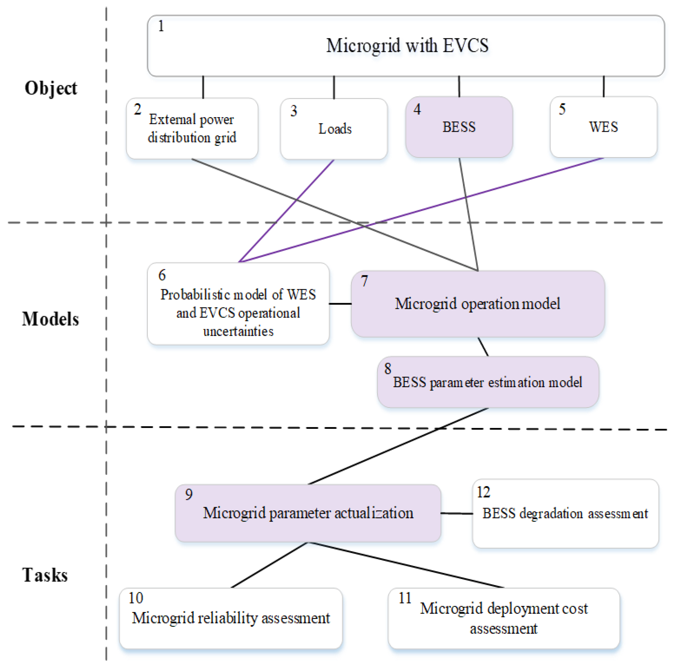
Figure 2.
Generalized Algorithm for Sizing EES and WPP with a Focus on Deficit-Free System Operation.
Figure 2.
Generalized Algorithm for Sizing EES and WPP with a Focus on Deficit-Free System Operation.
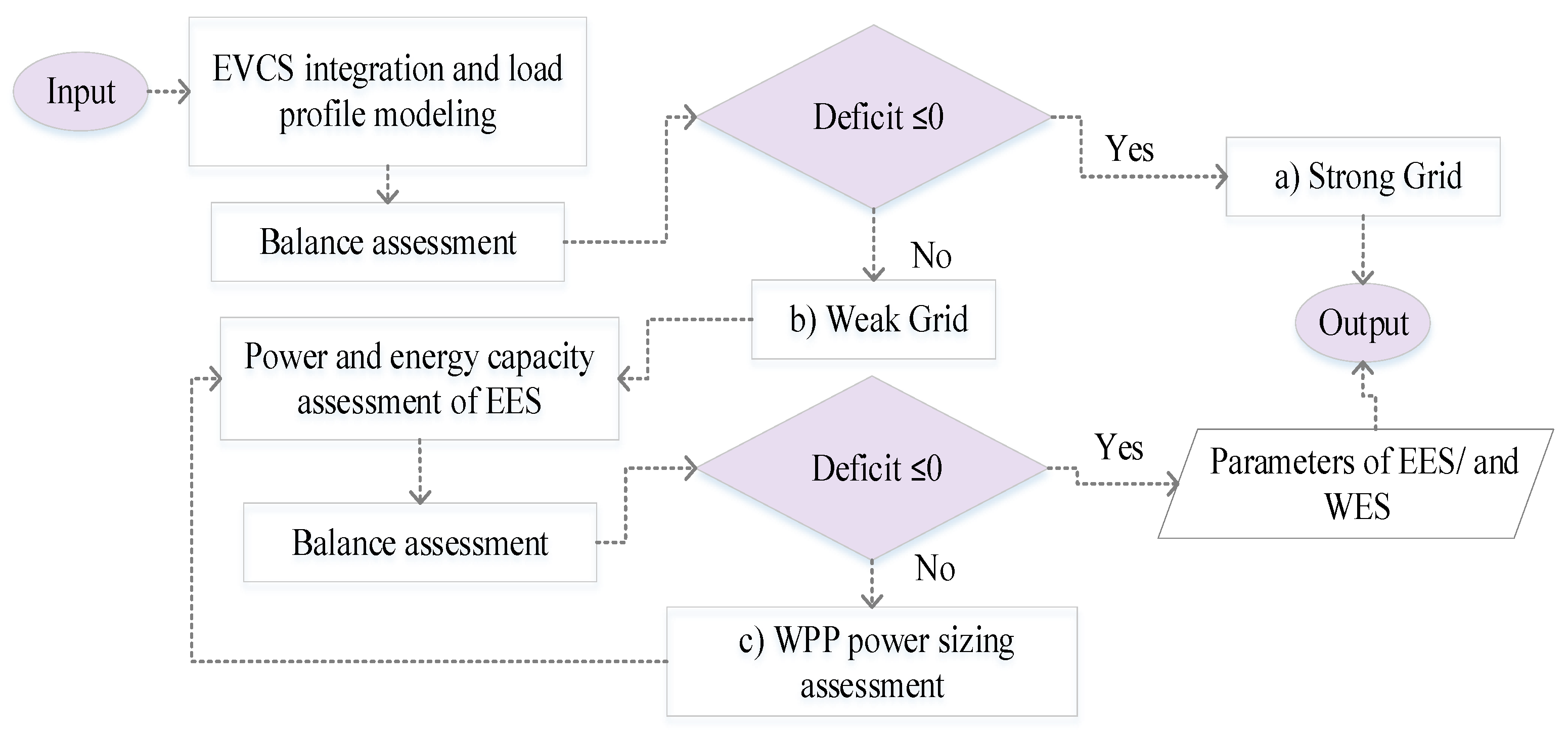
Figure 4.
The empirical graph of the power intensity of EV connections over a month.
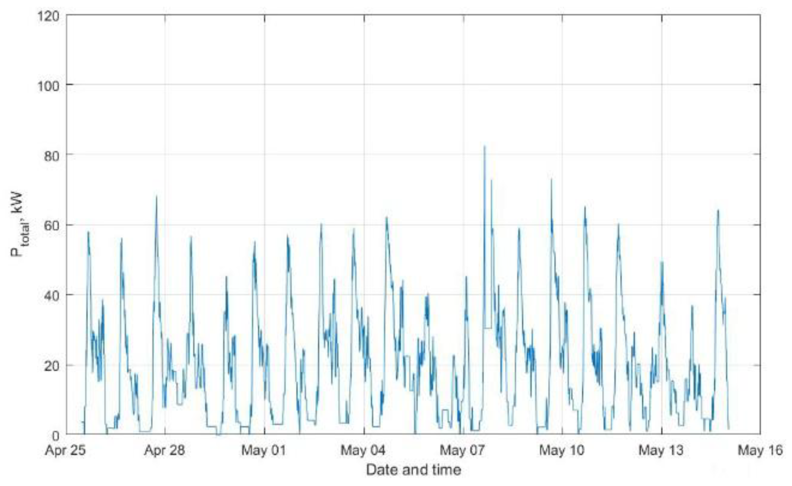
Figure 5.
The average daily empirical load graph of the EVCS.
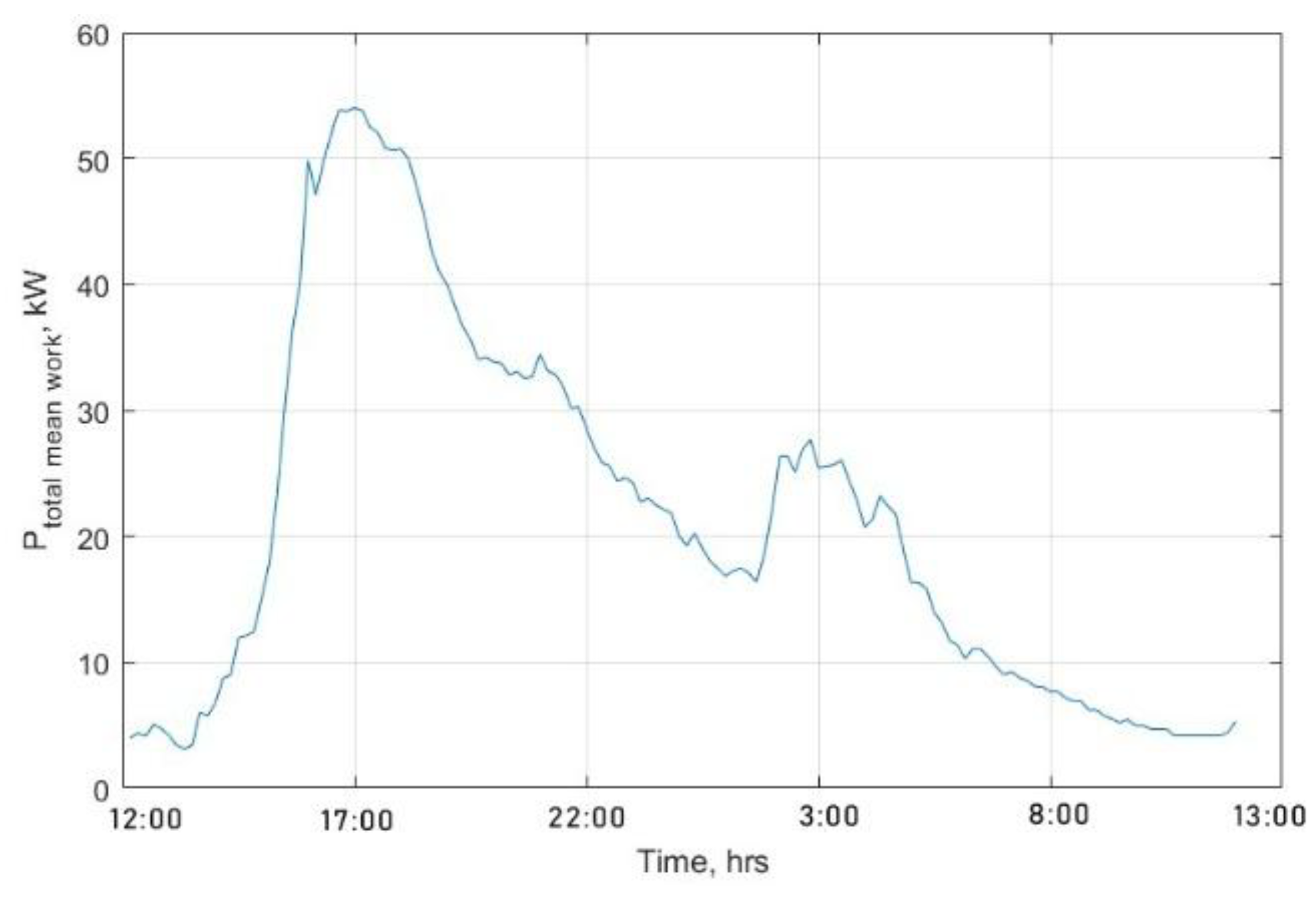
Figure 6.
Average Daily Profile and a Randomly Generated Day.
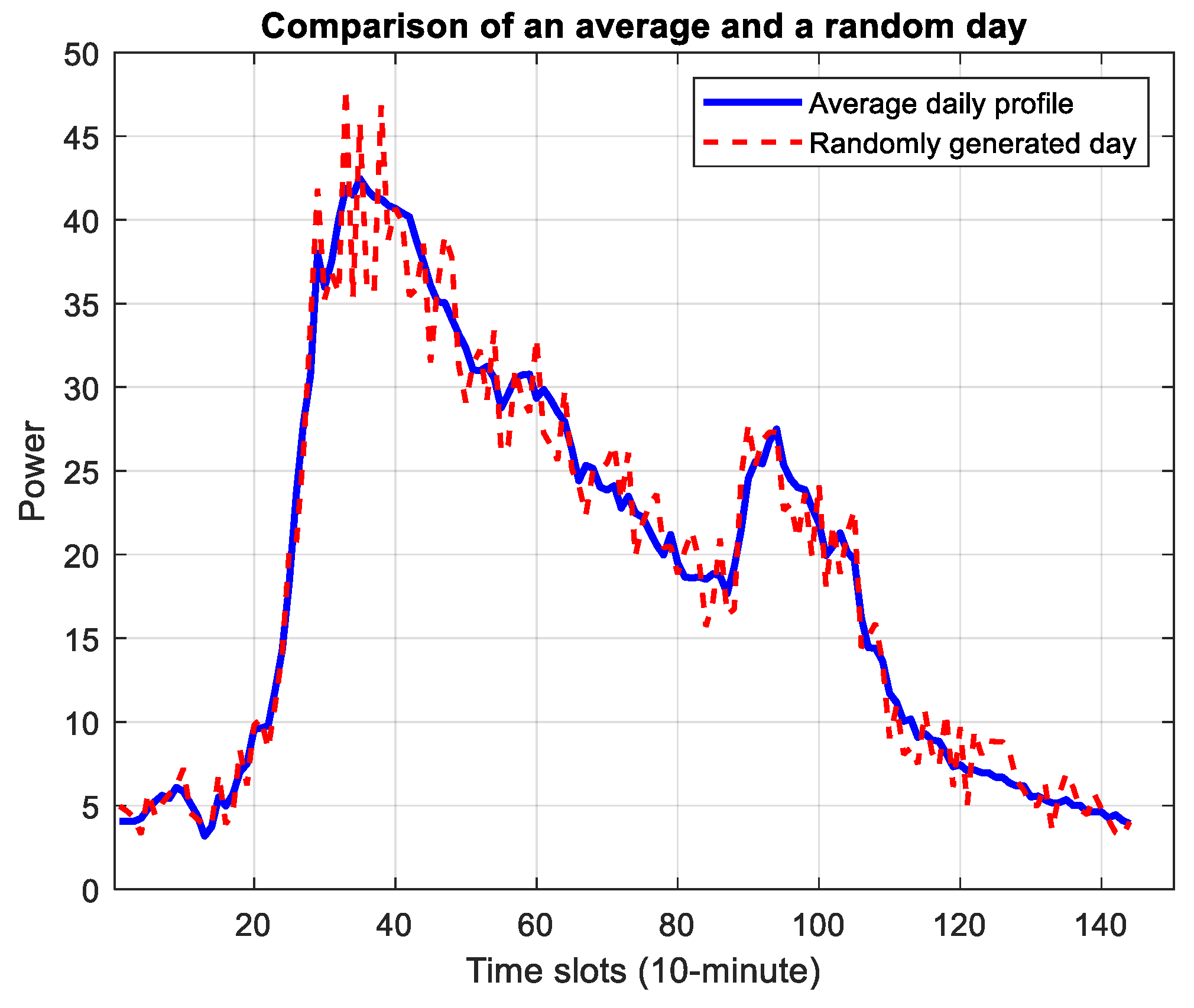
Figure 7.
Comparison of Actual and Synthetically Generated Daily Profiles.
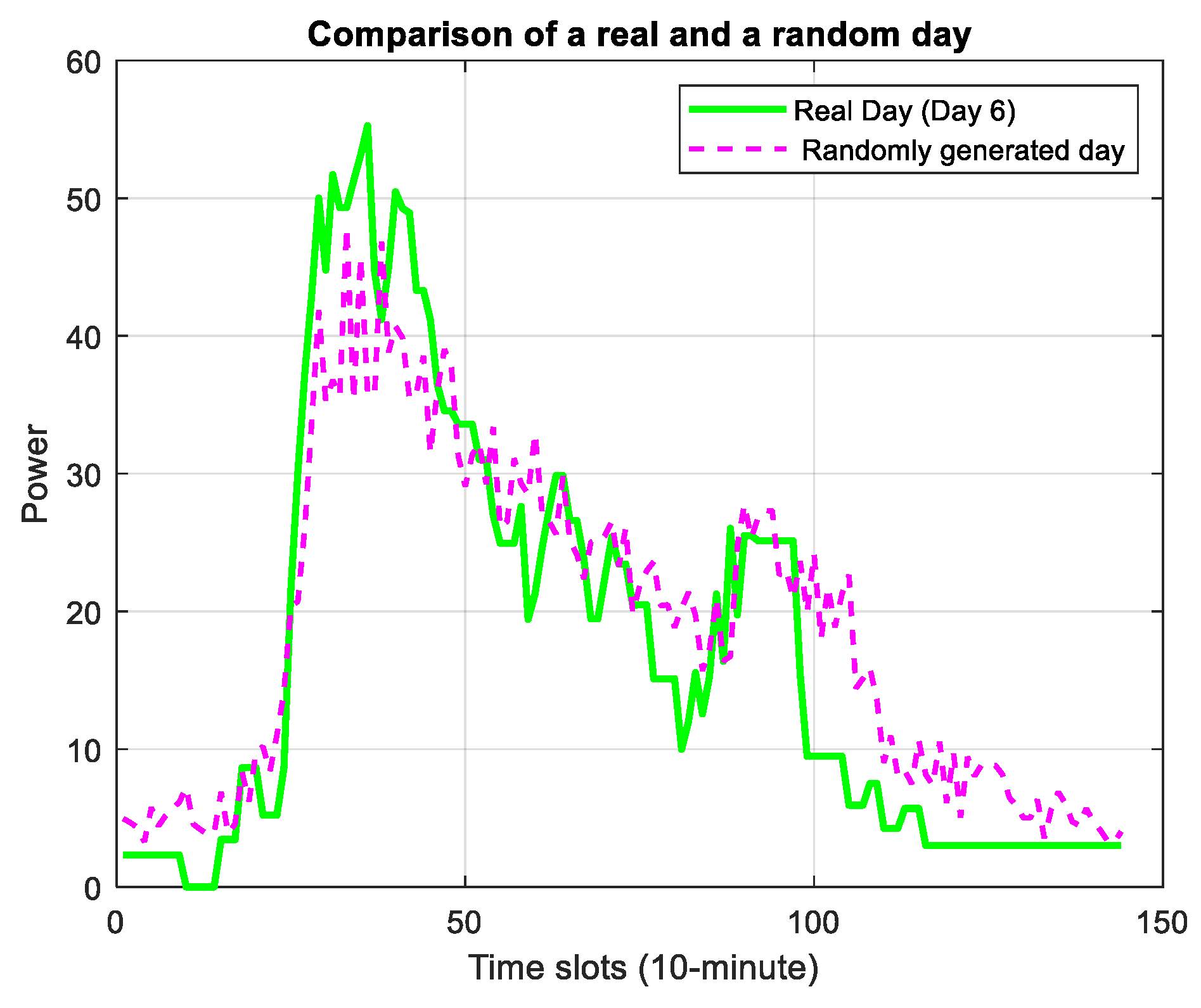
Figure 8.
Comparison of Averaged Profiles.
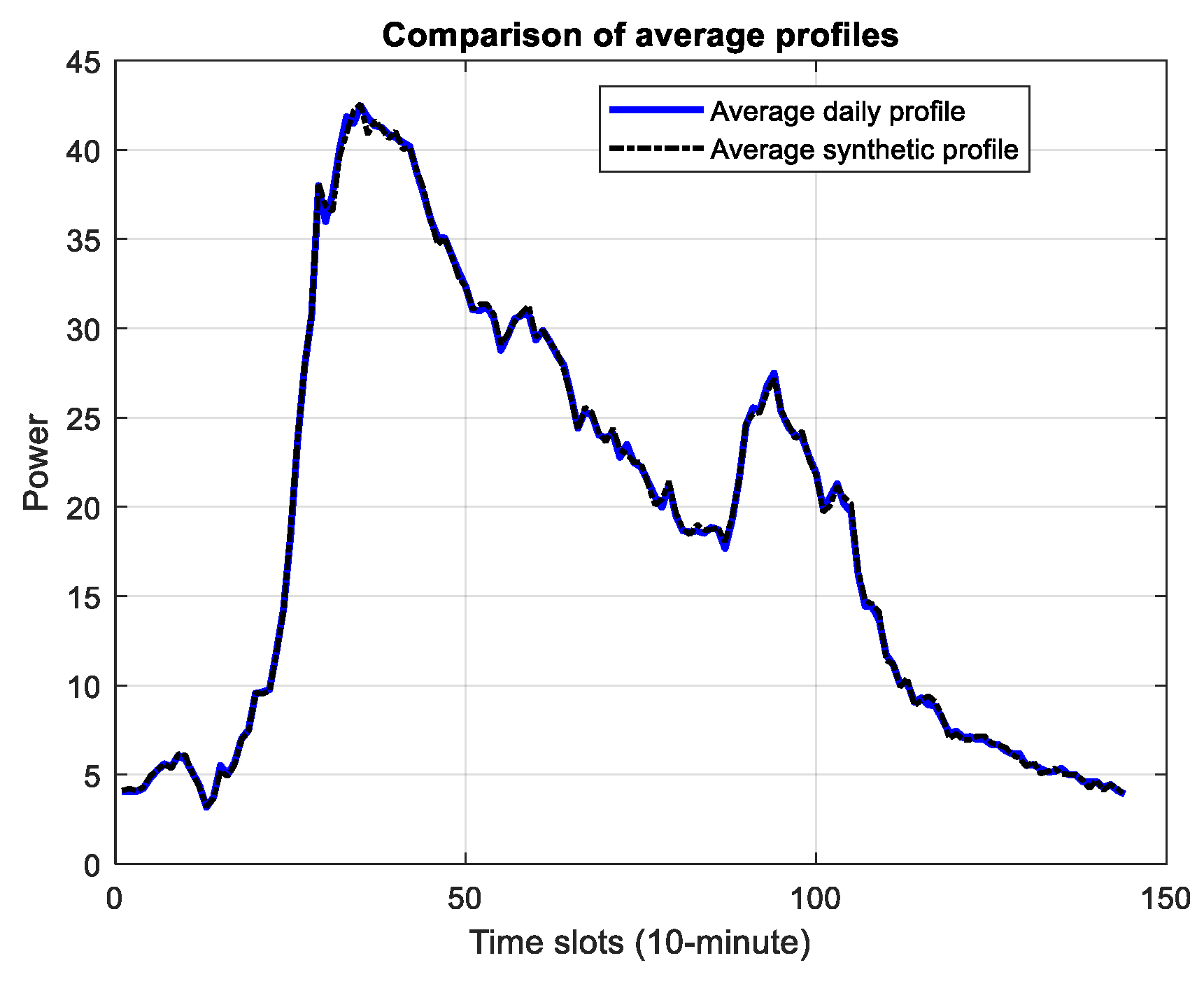
Figure 9.
Charging Start and End Times vs. Sequential Number of the Arriving EV.
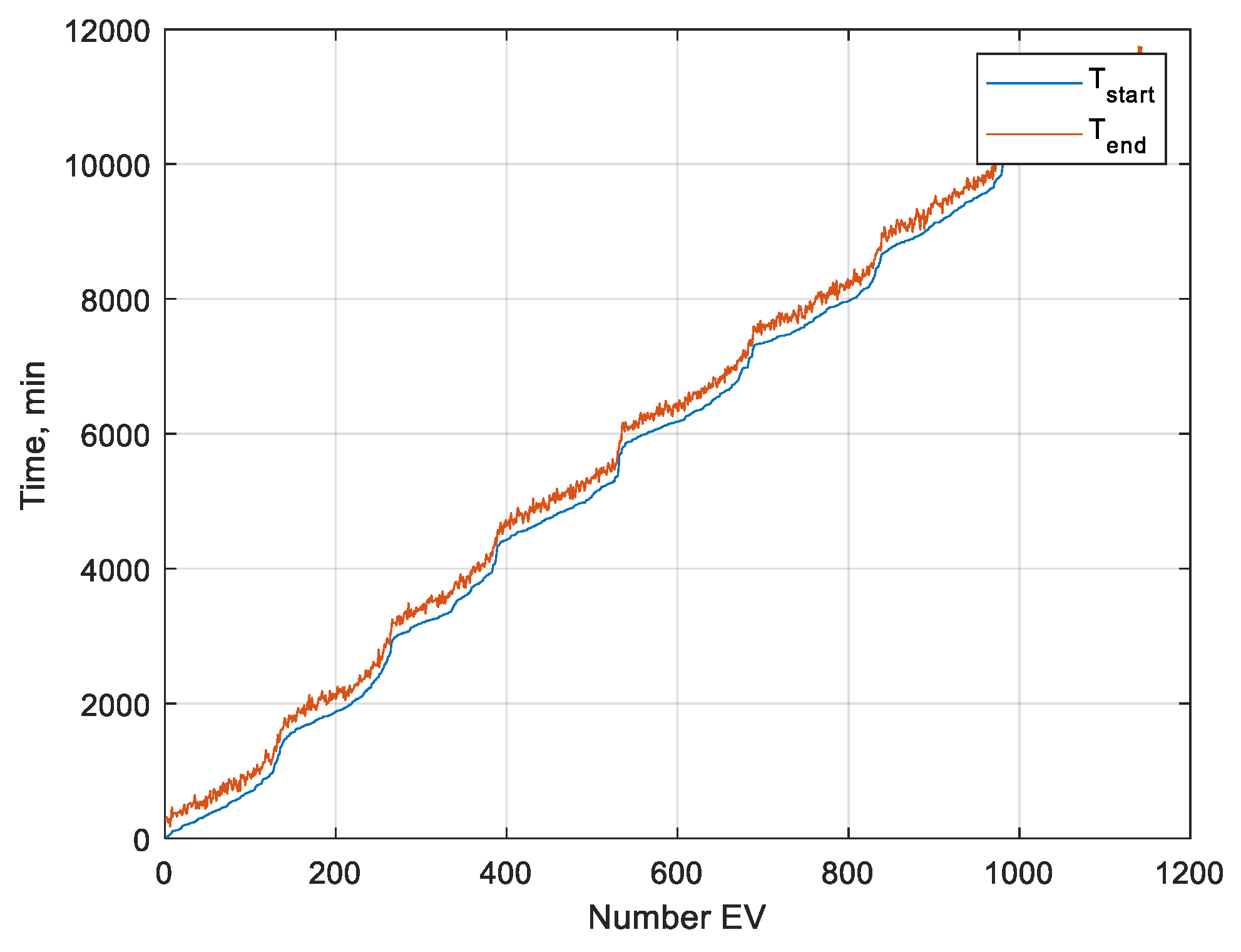
Figure 10.
Total EVCS Load Power Profile Over a Week.
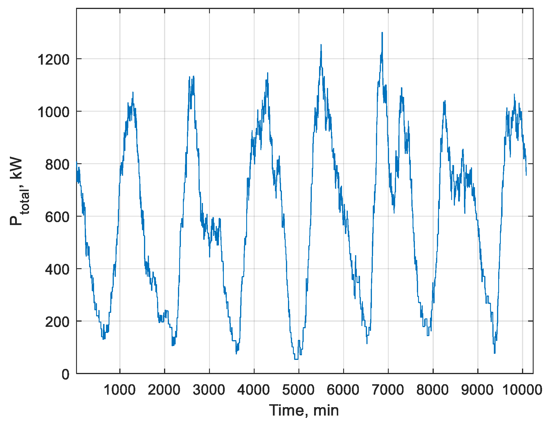
Figure 11.
Daily Load Profile.
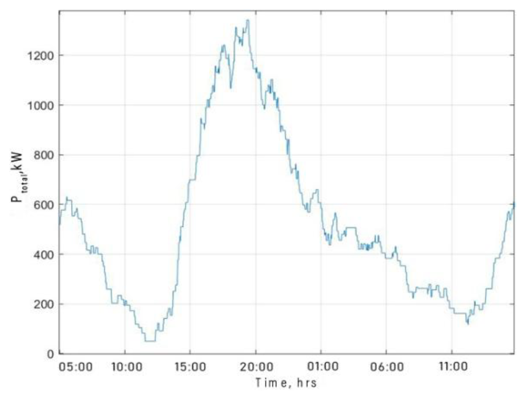
Figure 12.
Number of Simultaneously Charging Vehicles Over Time.
Figure 13.
Algorithm for Assessing WPP Generation.
Figure 14.
Diagram for Selecting EES Parameters Considering Three Criteria.
Figure 15.
Total Load of the Distribution Network and the EVCS at the Connection Point (Implementation Example).
Figure 15.
Total Load of the Distribution Network and the EVCS at the Connection Point (Implementation Example).
Figure 16.
Load Profile for Each Quantile.
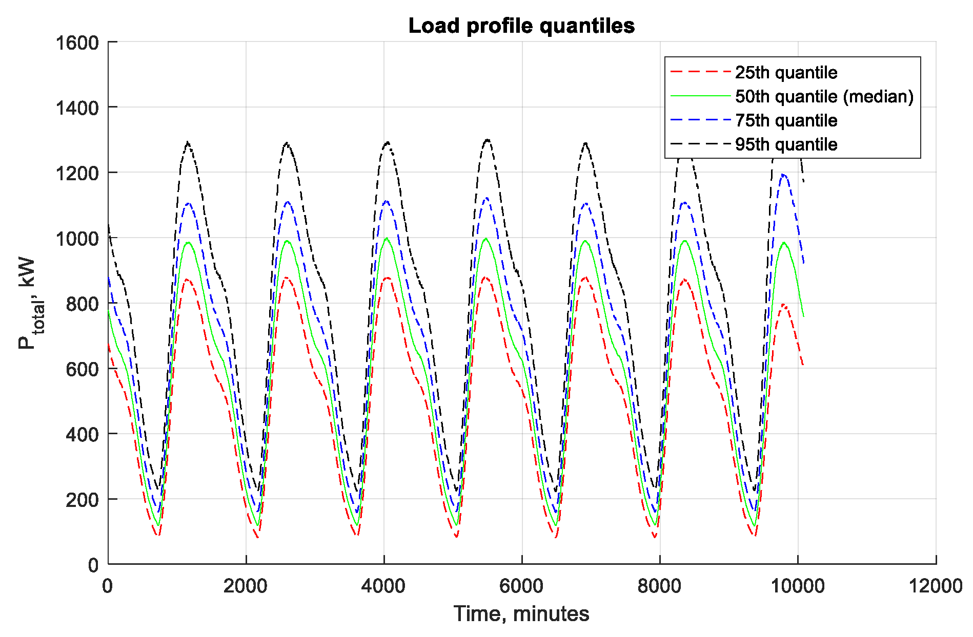
Figure 17.
EES Degradation.
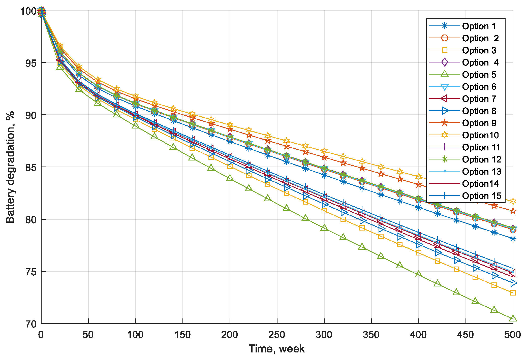
Figure 18.
Reliability Assessment of the Options.
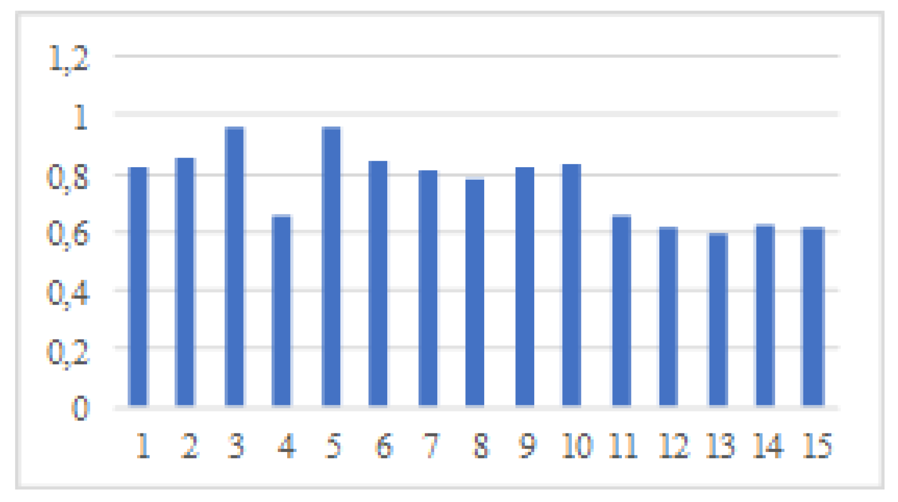
Figure 19.
Diagram for Selecting EES Parameters Based on Three Criteria.
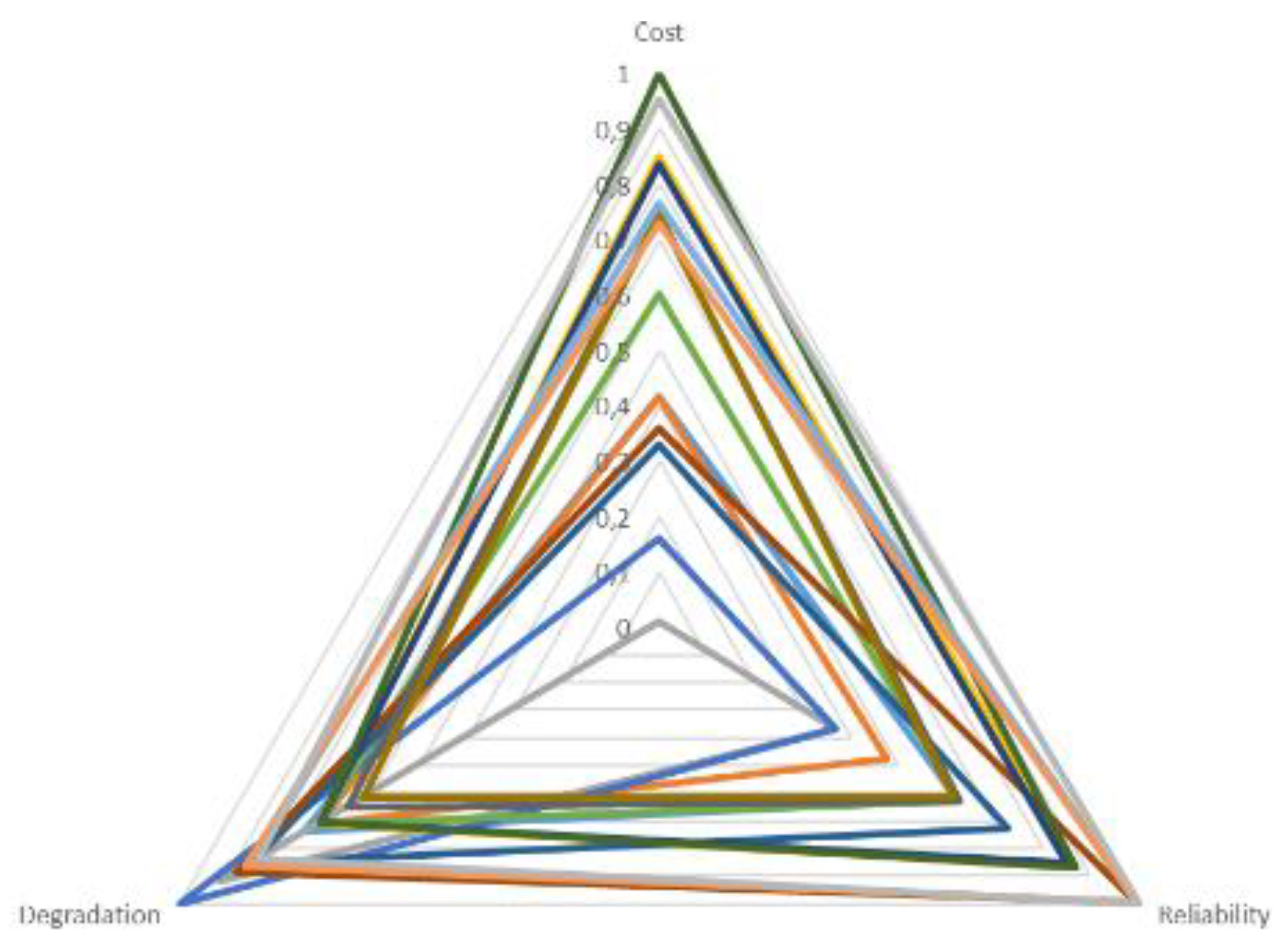

Table 1.
Calculation Results for the Microgrid Network Parameters.
| Options | Grid Capacity, MW | Load Capacity, MWh | WPP Capacity, MW | EES Power Rating, MW | EES Energy Capacity, MWh |
|---|---|---|---|---|---|
| 1 | 0.88 | 1.8 | 0.4 | 0.96 | 5.21 |
| 2 | 0.88 | 1.4 | 0.3 | 0.53 | 5.3 |
| 3 | 1.76 | 1.8 | 0 | 0.08 | 0.15 |
| 4 | 0.63 | 1.8 | 1.8 | 1.51 | 10 |
| 5 | 1,26 | 1.8 | 0 | 0.65 | 2.14 |
| 6 | 0.88 | 1.8 | 0.4 | 0.97 | 7.72 |
| 7 | 0.88 | 1.8 | 1 | 0.85 | 3.48 |
| 8 | 0.88 | 1.8 | 2 | 0.65 | 2.94 |
| 9 | 0.88 | 1.8 | 0.4 | 0.97 | 9.65 |
| 10 | 0.88 | 1.8 | 0.38 | 0.97 | 9.65 |
| 11 | 0.63 | 1.4 | 1.4 | 0.9 | 9.99 |
| 12 | 0.63 | 1.8 | 1.51 | 1 | 12 |
| 13 | 0.63 | 1.8 | 2 | 1 | 8.4 |
| 14 | 0.63 | 1.4 | 2 | 0.9 | 7.92 |
| 15 | 0.63 | 1.8 | 2 | 1.3 | 10.92 |
Disclaimer/Publisher’s Note: The statements, opinions and data contained in all publications are solely those of the individual author(s) and contributor(s) and not of MDPI and/or the editor(s). MDPI and/or the editor(s) disclaim responsibility for any injury to people or property resulting from any ideas, methods, instructions or products referred to in the content. |
© 2026 by the authors. Licensee MDPI, Basel, Switzerland. This article is an open access article distributed under the terms and conditions of the Creative Commons Attribution (CC BY) license.
Copyright: This open access article is published under a Creative Commons CC BY 4.0 license, which permit the free download, distribution, and reuse, provided that the author and preprint are cited in any reuse.


