Tensor Logic of Embedding Vectors in Neural Networks

1. Introduction

The quest for a universal calculus of thought, or characteristica universalis, has been the driving force of formal logic since Leibniz (1677)[32]. From the early insights of the Port-Royal logic (La Logique, ou l’Art de penser, 1662), which viewed language as a logical construction rather than a mere sequence of symbols, to a stable definition of predicative logic by Hilbert and Ackermann (1928) [6,10,18], the objective has been to map the structure of natural language onto a rigorous formal system.

A pivotal moment occurred in the 20th century with Reichenbach’s (1947) language analysis within the predicative logic setting, followed by the groundbreaking work of Richard Montague in the 1970s. Richard Montague, a student of Alfred Tarski, attempted to treat “English as a formal language” by employing $\lambda$-calculus and intensional logic [26,27,28]. However, while rigorous, Montague’s framework often led to excessive complexity that struggled to scale within the emergent field of computational linguistics.

Recently, artificial neural networks, introduced since the first stage of computer science developments [24], have achieved great successes combining computer science, cognitive science, and linguistics, by developing methods of machine learning that train the artificial neural networks to acquire complex abilities [1,3,8,11,12,13,14,15,25,29,36,37]. Probably, the most surprising success is the new generation chatbots (ChatGPT-OpenAI) [30], (Gemini-Google), (Claude-Antropic), (Copilot-Microsoft), …based on LLM (Large Language Model) transformers [11,14,23]. They are neural networks Pre-trained to Generate natural language texts by Transforming them into numerical vectors (GPT), called embedding vectors, in multidimensional semantic spaces. This paper suggests the possibility of combining the logical representation of natural language with the geometric perspective of transformers [2,7,23,38]. This would add a deeper understanding of texts, overcoming the current limitations of chatbots [9,34], and pushing towards future systems of artificial cognition [31], where the interplay between cognition and logical representation surely has a crucial role [20,22].

The paper introduces the Functional Language Logic (FLL), an evolution of Montague’s functionalism to the European linguistic tradition of discourse logic. As detailed in previous works [17,19,21], FLL treats every lexical unit as a noeme –a functional operator– rather than a static notion. The primary innovation presented here is the translation of FLL into T-FLL, a tensor-based manifold, providing a bridge between symbolic precision and the continuous vector spaces of modern Large Language Models (LLMs). By mapping logical operators onto tensor operations, we propose a path toward a "Geometric Logic" that can ground the statistical power of LLM Transformers in formal necessity.

2. Church Type Theory

The formal foundation of FLL lies in Church’s Simple Theory of Types (1940) [5]. We adopt a dotted notation for functional abstraction (Church’s $\lambda$-abstraction): $x.E\left(x\right)$, where $E\left(x\right)$ is an algebraic expression containing the variable x. The application mechanism follows the $\beta$-rule identity, according to Church’s terminology, which formalizes Leonard Euler’s concept of function in Introductio in Analysin in Infinitorum (1748), where the notation for function application is introduced, writing the argument to which the function applies inside parentheses on the right of the function symbol:

$$(x.E(x\left)\right)\left(a\right)=E\left(a\right)\left(\beta rule\right)$$

(1)

where $E\left(a\right)$ denotes the evaluation of the expression $E\left(x\right)$ in correspondence with the value a of x. Whence:

$$x.E\left(x\right)=y.E\left(y\right)\left(\alpha rule\right)$$

and:

$$x.E_1\left(x\right)=x.E_2\left(x\right)\left(\eta rule\right)$$

iff $x.E_1\left(x\right)\left(a\right)=x.E_2\left(x\right)\left(a\right)$ for all values a of variable x.

Constants, Variables, and Expressions, built by means of some primitive functions, are typed. A Type $\tau$ is a category, or a symbolic mark associated with an expression E by a type assignment $E:\tau$. The typing rule for functional abstraction states that when $x:\tau$ and $E\left(x\right):\sigma$, then $x.E\left(x\right):(\tau \to \sigma )$ (this means that $(\tau \to \sigma )$ is the type of functions from elements of type $\tau$ to elements of type $\sigma$). The corresponding typing rule for functional application states that when $x:\tau$ and $f:(\tau \to \sigma )$, then $f\left(x\right):\sigma$.

The type $ind$ is assigned to basic elements, called individuals, while $bool$ is the type of truth (or boolean) values $\top ,\perp$.

A basic predicate is a function of type $(ind\to bool)$, which we abbreviate by $pred$.

If P is a predicate, then $\left\{x\right|P\left(x\right)\}$ is the class of elements satisfying P.

If A is a class of elements of type $\tau$, then $A:\left\{\tau \right\}$. Constants of individuals ($a,b,\dots$), predicates ($P,Q,\dots$), and classes ($A,B,\dots$), and expressions equated to them are called substantives.

An infinite hierarchy of types can be built on individuals and Boolean types: $(ind\to bool)$, $\left\{ind\right\}$, $(ind\to (ind\to bool\left)\right)$, $\left(\right(ind\to bool)\to (ind\to bool\left)\right)$, $\left(\right\{ind\}\to bool)$, …

For any type, we assume a denumerable set of constants and variables of that type.

The logical order of a type is the maximum number of consecutive open parentheses and braces that occur in the type.

Lambda abstraction enables us to represent any function with multiple arguments using monadic functions. Let us consider a case of three arguments:

$(x_1,x_2,x_3).P(x_1,x_2,x_3)=$

$x_1.((x_2,x_3).P(x_1,x_2,x_3))=$

$=x_1.(x_2.(x_3.P(x_1,x_2,x_3)))$

Namely, for any three arguments $a_1,a_2,a_3$:

$x_1.(x_2.(x_3.P(x_1,x_2,x_3)))\left(a_1\right)=x_2.(x_3.P(a_1,x_2,x_3))$

$x_2.(x_3.P(a_1,x_2,x_3))\left(a_2\right)=x_3.P(a_1,a_2,x_3)$

$x_3.P(a_1,a_2,x_3)\left(a_3\right)=P(a_1,a_2,a_3)$

Truth values ⊤ and ⊥ are constants that can be considered as special propositions. Within Church Type Theory, we can easily reconstruct all the predicative logic of boolean connectives and quantifiers ($P,Q$ denote propositions) [21]:

$\neg \top =\perp$  and  $\neg \perp =\top$

$P\to Q=\perp$  iff  $P=\top$  e  $Q=\perp$

$P\wedge Q=\top$ iff $P=\top$ e $Q=\top$

$P\vee Q=\perp$ iff $P=\perp$ e $Q=\perp$

$P\leftrightarrow Q$  iff  $P=Q$

$\forall xP\left(x\right)=(P=x.\top$)

$\exists xP\left(x\right)=\neg (P=x.\perp )$

3. Functional Language Logic (FLL)

FLL formalism is rooted in Church’s type theory. Its main idea is the transformation of a given sentence into a noematic formula built with noemes, which are predicates associated with the words of a fixed language. Noemes are combined using some logical operators, and the noematic formula results in a list of pedications or equations. A predication consists of an application of a monadic predicate to an argument. An equation consists of a constant equated to an expression. Constants can be individual ($a,b,\dots$), predicative ($P,Q,\dots$), or collective ($A,B,\dots$) (classes). The type of predicates $(ind\to bool)$ is shortly called $pred$. We call hyperpredicates the functions of type $(pred\to bool)$ and adpredicates the function of type $(pred\to pred)$ (2-hypertredicates have type $\left(\right(pred\to bool)\to bool)$, and 2-adpredicates have type $\left(\right(pred\to pred)\to pred)$). The hierarchies of hyperpredicates and adpredicates can be extended to any level.

In FLL, boolean connectives and quantifiers are also operators on monadic predicates (↔ is predicate equality):

$\neg P=x.\neg P\left(x\right)$

$(P\to Q)=x.P\left(x\right)\to Q\left(x\right)$

$(P\wedge Q)=x.P\left(x\right)\wedge Q\left(x\right)$

$(P\vee Q)=x.P\left(x\right)\vee Q\left(x\right)$

$(\forall P)=(P=x.\top$)

$(\exists P)=(P=\neg (x.\perp \left)\right)$

We will show that twenty FLL operators can express any sentence by a noematic formula (see Table 1). FLL operators are divided into six groups: predicative, copredicative, descriptive, connective, assertive, and numerical.

The predicative operators of The FLL are the predication, that is, the application of a monadic predicate to an argument, and ^{^}, which is the predicative abstraction or hyperpredication. This operator applies to a predicate, for example $Walk$, and expresses the second-order property $\widehat{Walk}$ that is common to the predicates that imply the property of walking. Therefore:

$$\widehat{Walk}\left(P\right)=(P\to Walk)$$

whence: $P\left(a\right)\to Walk\left(a\right)$.

The formal definition of hyperpredication is (X predicative variable):

$$\widehat{P}=X.(X\to P)$$

which equates an implication into a predication. In this definition, it is essential to have the functional abstraction, predicate variables, and monadic predicates. The classical Aristotelian barbara syllogism becomes completely adherent to its linguistic form when it is stated in FLL using predicative abstraction ($Socrates$ is a predicate such that $Socrates\left(a\right)$ means that there is an individual a having the proper noun “Socrates”):

$$\widehat{Mortal}\left(Man\right)\wedge \widehat{Man}\left(Socrates\right)\to \widehat{Mortal}\left(Socrates\right)$$

The copredicative operators of FLL are: (direct) complementation, modification, hypercomplementation (indirect complementation), and specification.

Complementation is the operator _ (in suffixed notation) that transforms a predicate that has two arguments into a monadic predicate:

$$(x,y.P(x,y\left)\right)\_b=x.P(x,b)$$

Whence: $Love\_b\left(a\right)=Love(a,b)$.

Specification, which in traditional linguistic analysis is a kind of complementation, deserves a different formalization because the logical operator that it expresses has a different logical nature. Namely, given a constant c, the specification operator $\langle |$ gives $\langle c|$, which is the monadic predicate expressing a relation of pertinence, relationship, affinity, inclusion, …with the individual c, which generically corresponds to the linguistic expression “of c”.

A modification $Q\left[P\right]$, where Q is a predicate modifying the predicate P, is the new predicate with characteristics of P changed by the influence of Q. For example, $Good\left[Policeman\right]$ is a quality that is not the conjunction of $Good$ and $Policeman$, because in “good policeman” the influence of “good” is specific to the meaning of policeman, and completely different from a “good father”.

Indirect complementation in FLL is realized by hypercomplementation, because a linguistic element, which we call completer, say it $Comp$ (in many languages, $Comp$ is a preposition), is considered as a function taking an individual b (the complement) and providing $Comp\_b$, a second-order property. For example, the proposition $With$ becomes $With\_b$, then when $\widehat{Go}\left(P\right)$, the predication $With\_b\left(P\right)$ adds to P the quality of going with b. Therefore, to say that a goes with b, we can write: $P\left(a\right)$ ; $(\widehat{Go}\wedge With\_b)\left(P\right)$, or simpler:

$$\widehat{Go}\left(P\right);With\_b\left(P\right);P\left(a\right)$$

Another possibility is to consider $With\_b$ a modifier, by writing $P\left(a\right)$ together with:

$$\widehat{With\_b\left[Go\right]}\left(P\right)$$

Suitable axioms of FLL could regulate these semantic equivalences (and analogous ones), but we do not pursue this direction further because it would take us far from the main topic of our discourse. However, we want to remark on two important general aspects:

1) Very often, linguistic elements can assume different types, depending on the linguistic construction they are involved in ($Good$ can be a predicate, $Good\left(a\right)$, or a modifier of a predicate in $Good\left[Policeman\right]$).

2) Predicative constants differ from noemes, because they are contingent predicates, or particular instances of noemes, “living” in the context of the noematic formula they belong to, while noemes are persistent predicates with a stability related to the cognitive system they represent. For this reason, we can write $With\_b\left(P\right)$, but cannot write $With\_b\left(Go\right)$. Namely, $With\_b$ is not a property of noeme $Go$. Still, it may be a property of a particular instance of going, which is realized in a specific context and asserted in a sentence associated with that context.

The descriptive operators of FLL are: ι, ϵ, λ, =, the last ones are the functional abstraction and the equation, which assigns to a constant an expression (FLL substantivation). The first two operators correspond to the determinative article “the”, and to the indefinite pronoun “any”, respectively.

Operators $\iota ,ϵ$ are due to Giuseppe Peano and David Hilbert [33,40]. Peano’s $\iota$ when applied to a predicate denotes the unique value satisfying it (if such a value does not exist, or more than one value satisfies the predicate, all predications on it are false). Actually, the FLL meaning of $ϵ$ is somewhat different from Hilbert’s original operator (denoted by the $\epsilon$ variant of $ϵ$ [40]). Namely, $ϵ$ applied to a predicate denotes a randomly chosen argument that satisfies it, but if no such value satisfies the predicate, all predications on it are false.

Operator $ϵ$ enables elimination of variables in $\lambda$-expressions, by using symbol $ϵ$ with numerical indexes, intending that $ϵ$ occurrences with the same index replace occurrences of the same variable (${ϵ}_i$ stands for any individual), for example:

$$y.(x.\mathrm{\Phi }(x,y))={ϵ}_2.({ϵ}_1.\mathrm{\Phi }({ϵ}_1,{ϵ}_2))$$

The connective operators of FLL are: $\neg ,\to ,\wedge ,\vee$ (negation, implication, conjunction, and disjunction), which are the boolean connectives on propositions and monadic predicates.

The three assertive operators of FLL are: $\vDash ,?\vDash ,!\vDash$ (assertion, interrogation, exhortation).

Numerals 0, 1, 2, …are considered particular constants. The three numerical operators of FLL are: $(>1),n,n^{\circ }$, used for plurals, cardinal numbers, and ordinal expressions. The class abstraction$\left\{x\right|P\left(x\right)\}$, or simply $\left\{P\right\}$, can be considered a special case of pluralization.

Examples of noematic formulae representations are provided below to illustrate the descriptive precision of FLL [19,21]. We remark that predication is always realized with monadic (monoargumental) predicates.

• Example 1 (Predication, Modification, Assertion): “Giulio is a good boy”:

  $$Giulio\left(a\right);\vDash Good\left[Boy\right]\left(a\right)$$
  This means that there is an individual, denoted by a, who satisfies the predicate Giulio (being a proper noun, the predicate expresses the property of having the name `Giulio’). Then, the same individual satisfies the predicate Good boy, which is a modification of Boy. The predication prefixed by ⊧ is the main fact asserted by the sentence.
• Example 2 (Complementation): “Giulio loves Helen”:

  $$Giulio\left(a\right);Helen\left(b\right);\vDash Love\_\left(b\right)\left(a\right)$$
  In this case, we can proceed as in the previous example. Still, Love is a binary predicate (a transitive verb Love(x, y), expressing that the first argument loves the second one), therefore it is transformed into $Love\_\left(b\right)=x.Love(x,b)$. The operator _ is (direct) complementation.
• Example 3 (Hyperpredication) “Giulio loved Helen”:

  $$Giulio\left(a\right);Helen\left(b\right);\widehat{Love}\left(P\right);Past\left(P\right);\vDash P\_\left(b\right)\left(a\right)$$
  The operator ^{^} of predicative abstraction applies to $Love$, expressing the second-order property common to the predicates that imply the property of loving. The predicative constant P denotes a predicate that implies loving, it is in the past, and holds on a when its object is b.
• Example 4 (Complementation, Specifcation, Hypercomplementation):
  “Helen was going home by her bike”:

  $$Helen\left(a\right);Home\left(b\right);Bike\left(c\right);\widehat{Go\_b}\left(P\right);(Past\wedge Progr)\left(P\right);\langle a|\left(c\right);By\_c\left(P\right);\vDash P\left(a\right)$$
  In this formula, the complementations $Go\_b$, the hypercomplementation $By\_c$, and the specification operators occur.
• Example 5 (Distributive Sentence):
  “The boys entered the classroom two at a time”

  $$A=\iota (>1)\left[Boy\right];Classroom\left(b\right);\widehat{Enter\_b}\left(P\right);(Past\wedge Continuative)\left(P\right);2\_ϵTime\left(P\right);$$
  $\vDash P\left(A\right)$
  Here $(>1)\left[Boy\right]$ is the plural of $boy$ and $\iota$ is the determiner “the” (Peano’s operator), meaning that in the context of the sentence, there are some boys, univocally determined, denoted by the constant A of a class. The hypercomplementation $ϵTime\_2$ expresses the distributive aspect of the continuative action realized by the entering of P, where, at any step, 2 boys enter.
• Example 6 (Donkey Sentence): “Any man loves a woman who loves him”

  $$b=ϵMan;Woman\left(a\right);Love\_b\left(a\right);\vDash Love\_a\left(b\right)$$
  In this sentence, a pronoun falls in the scope of an indefinite/ distributive pronoun. The term “Donkey Sentence” derives from the medieval philosopher Walter Burleigh, whose example sentences contain mention of donkeys (see section 6). In the noematic formula above, Hilbert’s $ϵ$ operator occurs, which expresses a choice of a value satisfying a predicate. The following formula represents “Every man loves a woman who loves him”:

  $$X=ϵ\widehat{Love};b=ϵMan;Woman\left(a\right);X\_b\left(a\right);\vDash X\_a\left(b\right)$$
• Example 7 (Relative Sentence):
  “Giulio is searching for the pen that Helen gave him”
  $Giulio\left(a\right)$ ; $Helen\left(b\right)$ ; $Present\wedge Progressive\left(P\right)$ ; $\widehat{Search-for}\left(P\right)$ ;
  $\widehat{Give}\left(Q\right)$, $Paste\left(Q\right)$ ; $R=x.Q\_x\left(b\right)$ ; $c=\iota (R\wedge Pen)$ ; $\vDash P\_c\left(a\right)$
  Here, Giulio is searching for a pen that satisfies a specific property expressed by a $\lambda$-expression.
• Example 8 (Without Complementation): “Yesterday I was walking without shoes”

  $$Me\left(a\right);Yesterday\left(P\right);b=ϵ\left(2\left[Shoe\right]\right);\widehat{Walk}\left(P\right);\widehat{\neg Wear\_b}\left(P\right);\vDash P\left(a\right)$$
  Here, predicative abstraction is applied after a direct complementation and negation.
• Example 9 (Consecutive Sentence): “The suitcase is so heavy that I cannot carry it”
  $Me\left(a\right);b=\iota \left(Suitcase\right);(\langle b|\left[Weight\right]\left)\right(c);d=ϵ(Weight\left(x\right)\wedge x.Able\left[Bring\right]\_x\left(a\right));$
  $\vDash Weight\left[Greater\right]\_d\left(c\right)$
  This formula says that the weight of the suitcase is greater than any weight that I can bring.
• Example 10 (Temporal Subordination):
  “The boys were entering while the teacher was speaking”
  $A=\iota \left(\right(>1\left)\right[Boy\left]\right)$ ; $Teacher\left(b\right)$ ; $\widehat{Enter}\left(P\right)$ ; $\widehat{Speak}\left(Q\right);$ $Past\wedge Progressive\left(P\right);$
  $Past\wedge Progressive\left(Q\right)$ ; $P^{\prime }=P\left(A\right)$ ; $Q^{\prime }=Q\left(b\right)$ ; $\vDash While\_Q^{\prime }\left(P^{\prime }\right)$
  The temporal subordination is realized by two constants denoting the propositions and then by expressing the temporal relation by using complementation.
• Example 11 (Interrogation): “Where are you going?”
  $You\left(a\right)$ ; $Place\left(b\right)$ ; $\widehat{Go}\left(P\right)$ ; $(Present\wedge Progressive)\left(P\right)$ ; $\vDash b?P\_b\left(a\right)$
  This interrogation expresses the argument b for which a further detailed description is requested.
• Example 12 (Exhortation): “Go home”
  $You\left(a\right)$ ; $Home\left(b\right)$ ; $\widehat{Go}\left(P\right)$ ; $Present\left(P\right)$ ; $a!\vDash P\_b\left(a\right)$
  This exhortation highlights the subject a, who is requested to fulfill the order (making the sentence true).

The following table (Table 1) summarizes the 20 fundamental operators of FLL ($subst$ is the polymorphic type of any constant or descriptive expression).

Table 1. The 20 fundamental operators of Functional Language Logic (FLL).

#	Operator	Logical Designation / Functional Type
1	$P\left(s\right)$	Predication (s satisfies the property P) $P:(subst\to bool)$
2	$s=E$	Equation (expression E is assigned to substantive s): $(c:\tau )\Rightarrow (E:\tau )$
3	$\widehat{P}$	Hyperpredication: ^$:(pred\to (pred\to bool))$
4	$x.E\left(x\right)$	$\lambda$-abstraction: $(x:\tau ),\left(E\right(x):\sigma )\Rightarrow (x.E(x):(\tau \to \sigma \left)\right)$
5	¬	Negation : $(pred\to pred)$
6	→	Implication : $(pred\to (pred\to pred\left)\right)$
7	∧	Conjunction (Predicative Conjunction) : $(pred\to (pred\to pred\left)\right)$
8	∨	Disjunction (Predicative Disjunction) : $(pred\to (pred\to pred\left)\right)$
9	$P\_s$	Complementation (Direct): $\_:(pred\to (subst\to pred\left)\right)$
10	$Prep\_s\left(P\right)$	Hypercomplementation : Prep_ : $(subst\to (pred\to bool\left)\right)$
11	$\langle s|$	Specification: $\langle c|$ is the predicate “of s”; $\langle |:(subst\to pred)$
12	$Q\left[P\right]$	Modification (Noematic warping); $-[-]:(pred\to (pred\to pred\left)\right)$
13	$\iota P$	Determination ; $\iota :(pred\to subst)$ ($\iota Boy$ = “the boy”)
14	$ϵP$	Indetermination $ϵ:(pred\to subst)$ ($ϵBoy$ = “any boy”)
15	⊧	Assertion (Focus Proposition); $\vDash :(bool\to bool)$
16	$?\vDash$	Interrogation $?\vDash :(bool\to bool)$
17	$!\vDash$	Exhortation $!\vDash :(bool\to bool)$
18	$(>1)\left[P\right]$	Pluralization $(>1)\left[Boy\right]$ (Boys); $(>1)\left[\right]$ and $\left\{\right\}:(pred\to (\left\{ind\right\})$
19	$n\left[P\right]$	Numeration $2\left[Boy\right]$ (two boys); $2\left[\right]:(pred\to (\left\{ind\right\}\left)\right)$
20	$n^{\circ }\left[P\right]$	Seriation $2^o\left[Boy\right]$ (second boy); $2^{\circ }\left[\right]:(pred\to ind)$

Table 1. The 20 fundamental operators of Functional Language Logic (FLL).

#	Operator	Logical Designation / Functional Type
1	$P\left(s\right)$	Predication (s satisfies the property P) $P:(subst\to bool)$
2	$s=E$	Equation (expression E is assigned to substantive s): $(c:\tau )\Rightarrow (E:\tau )$
3	$\widehat{P}$	Hyperpredication: ^$:(pred\to (pred\to bool))$
4	$x.E\left(x\right)$	$\lambda$-abstraction: $(x:\tau ),\left(E\right(x):\sigma )\Rightarrow (x.E(x):(\tau \to \sigma \left)\right)$
5	¬	Negation : $(pred\to pred)$
6	→	Implication : $(pred\to (pred\to pred\left)\right)$
7	∧	Conjunction (Predicative Conjunction) : $(pred\to (pred\to pred\left)\right)$
8	∨	Disjunction (Predicative Disjunction) : $(pred\to (pred\to pred\left)\right)$
9	$P\_s$	Complementation (Direct): $\_:(pred\to (subst\to pred\left)\right)$
10	$Prep\_s\left(P\right)$	Hypercomplementation : Prep_ : $(subst\to (pred\to bool\left)\right)$
11	$\langle s|$	Specification: $\langle c|$ is the predicate “of s”; $\langle |:(subst\to pred)$
12	$Q\left[P\right]$	Modification (Noematic warping); $-[-]:(pred\to (pred\to pred\left)\right)$
13	$\iota P$	Determination ; $\iota :(pred\to subst)$ ($\iota Boy$ = “the boy”)
14	$ϵP$	Indetermination $ϵ:(pred\to subst)$ ($ϵBoy$ = “any boy”)
15	⊧	Assertion (Focus Proposition); $\vDash :(bool\to bool)$
16	$?\vDash$	Interrogation $?\vDash :(bool\to bool)$
17	$!\vDash$	Exhortation $!\vDash :(bool\to bool)$
18	$(>1)\left[P\right]$	Pluralization $(>1)\left[Boy\right]$ (Boys); $(>1)\left[\right]$ and $\left\{\right\}:(pred\to (\left\{ind\right\})$
19	$n\left[P\right]$	Numeration $2\left[Boy\right]$ (two boys); $2\left[\right]:(pred\to (\left\{ind\right\}\left)\right)$
20	$n^{\circ }\left[P\right]$	Seriation $2^o\left[Boy\right]$ (second boy); $2^{\circ }\left[\right]:(pred\to ind)$

4. The Tensors of Embedding Space

To understand how logic inhabits a neural network, we must first define the laws of the space where modern chatbots operate. Large Language Models (LLMs) project every linguistic unit into a high-dimensional manifold $\mathcal{N}$ known as the Embedding Vector space. This space is a geometric structure governed by multilinear algebra, based on tensors [2,4,7,16,23,38,39]. They are a powerful concept providing the right mathematical language for expressing physical theories. In this space, the “semantic mass distribution” supports the information flux of dialogs, making them adequate and productive.

Here, we distinguish between three types of entities:

• Vectors (${\mathbf{v}}^i$): Representing individual “points”. They are directed arrows in the manifold.
• Covectors ($P_i$): Also known as linear functionals or dual vectors. They represent “tests” or “filters”. When a covector meets a vector, they produce a scalar value through
  Contraction ($P_i{\mathbf{v}}^i$).
• Tensors (${\mathbf{T}}_j^i,{\mathbf{T}}_{ijk}$): Higher-order structures that act as operators. A tensor can rotate, scale, or warp one vector into another, representing the transformation of meaning (e.g., how an adjective modifies a noun).

4.1. Projections and Subspaces

The “intelligence” of a chatbot emerges from how it manipulates tensors:

• Contraction: This is the dot product that measures semantic similarity.
• Subspaces and Projections: A specific topic (e.g., “Mathematics”) occupies a slice or subspace of the manifold. To understand a word in context is to project its vector onto the relevant subspace.
• The Metric Tensor ($g_{ij}$): This is the “ruler” of the space. It defines the distance and the angle between vectors. In T-FLL, the metric determines the Semantic Density and the threshold of truth ($\theta$).

The core of the transformer models is the Scaled Dot-Product Attention, defined by the interaction of three matrices [39]: Query (Q), Key (K), and Value (V) (exponent T means transposition):

$$\mathrm{Attention}(Q,K,V)=\mathrm{softmax}\left({\displaystyle \frac{Q·K^T}{\sqrt{d_k}}}\right)·V$$

(2)

From an FLL perspective, this process can be viewed as a dynamic noematic weighting. The $Q{K}^T$ interaction determines the degree of correlation between noemes (e.g., how much the predicate Enter should “attend” to the predicate Boy in a sentence where both occur). This matrix product is then multiplied by the matrix V of the vectors representing the linguistic tokens of an input sentence. The resulting vector gives the attention coefficients of the input vectors, which, after a suitable normalization, determine the linear combination of the vectors of V, giving the global meaning of the input sentence. Therefore, the meaning emerges from the mutual interaction that contextualizes the embedding vectors recalled by the sentence and then combines their contextualizations. This mechanism is the key to a chatbot’s performance, turning the static knowledge incorporated in the embedding vectors into the dynamics of its conversational competence.

Transformers generate contextualized embeddings, which provide adequate outputs. Each vector in the hidden layers represents a “vortex” of information where the original noeme has been modified by its surroundings. This mechanism mirrors the FLL modification operator ($-[-]$), where the meaning of a predicate is warped by the presence of other noematic constraints in the sequence.

However, while Transformers achieve this through stochastic gradient descent, we will show that T-FLL provides a formal, interpretable protocol for these contextualizations.

5. From Logic Operators to Tensors

To bridge the gap between FLL and neural architectures, we must formalize the Noematic Space $\mathcal{N}$ as a multidimensional Hilbert space where semantic operations are expressed through multilinear algebra.

We assume the Noematic Space is equipped with a metric tensor $g_{ij}$, allowing for the calculation of distances between noemes. The semantic “coherence” of a formula is proportional to the density of the tensor field at the point of assertion.

The core innovation of T-FLL is the mapping of the logical act of judgment onto a geometric convergence. In FLL, the assertion operator (⊧) corresponds to a judgement localization on the Semantic Centroid ($\mathbf{C}$) within the Noematic Space, acting as the “field equation” of communication.

5.1. Predication as Scalar Product

To implement this convergence, each of the 20 FLL operators must be translated into its specific multilinear algebraic function. In T-FLL, we represent individual constants (e.g., $a,b,c$) as vectors $\mathbf{v}\in \mathcal{N}$, where $\mathcal{N}$ is a high-dimensional real Hilbert space. Conversely, noemes (predicates) are represented as elements of the dual space ${\mathcal{N}}^{*}$, acting as linear functionals (covectors).

The fundamental operation of predication, $P\left(a\right)$, is thus defined as the contraction:

$$\langle P,a\rangle =P_i{a}^i=\theta$$

(3)

where $\theta \in [0,1]$ and it corresponds to the degree of noematic adherence, or a truth value according to a truth-threshold discriminating values less than the threshold corresponding to ⊥ from greater values corresponding to ⊤.

5.2. Higher-Order Tensors

The modification operator $P\left[Q\right]$ is modeled as a $(1,1)$-tensor $M_j^i$ that acts on the covector $Q_j$ to produce a warped noeme $P_i^{\prime }$:

$$P_i^{\prime }=M_j^i{Q}_j$$

(4)

In a transformer, this corresponds to the linear transformations applied by the weight matrices $W_Q,W_K,W_V$ within each attention head. The complexity of natural language is captured by the rank of these tensors, where complementation and hypercomplementation (operators 9 and 10) are represented as successive contractions of indices in a tensor network.

Specification is the transformation of a vector into a covector, because a substantive s, that is, any constant denotation, is transformed into a predicate expressing the pertinence of s. We can imagine it in $\mathcal{N}$ as a cone centered at s. Specification and modification operators can be composed, and semantic relations can be stated between hypercomplementation specification and modification. Namely, when we say “Going with a bike” the predicate $Go$ is enriched or specialized by a further condition. In FLL terms, we have $\widehat{Go}\left(P\right)\wedge Bike\left(b\right)\wedge With\_b\left(P\right)$, in other words, P has the high-order property of going and of using b, which is a bike, as an instrument.

We define the assertion of a complex formula as the calculation of the “barycenter” of the involved noematic tensors. However, different from the standard attention mechanism, in T-FLL, this barycenter is computed by using tensors translating FLL operators. The assertion operator drives the centroid $\mathbf{C}$ computation to provide a focus in the noematic manifold for subsequent neural processing.

5.3. Mapping Anaphora via Persistent Indices

In FLL, equations assigning meaning to the constants solve the problem of anaphora resolution in tensor networks. Instead of relying on decaying positional encodings.

For example, during the computation of the donkey sentence (Example 6), the tensor contraction for Love is forced to reuse the register indexes $a,b$ ensuring that the “Man” and the “Woman” maintain their geometric identity across multiple attention heads in the semantic manifold $\mathcal{N}$.

6. Attention Driven by the Noematic Formula

The core innovation of T-FLL is the transition from a probabilistic attention model to a Noematic Machine. In this paradigm, the FLL formula is not a mere symbolic representation but the Execution Code that configures the tensor dynamics of the neural architecture.

Before the tensor calculation, a Noematic Parser has to translate the natural language input V into its corresponding FLL formula ${\mathrm{\Phi }}_V$. This can be done in several ways. Here, we do not enter into details, and a reasonable assumption is that a trained module is available to perform the passage from a sentence to the corresponding noematic formula.

For the Donkey Sentence “Any farmer who owns a donkey beats it”, the output could be the sequence:

$$a=ϵ\left(Farmer\right);Donkey\left(b\right);Own\_b\left(a\right);\vDash (Beat\_b(a\left)\right)$$

(5)

This formula acts as a Wiring Map, an instruction set that defines which noematic tensors must contract and in what order.

In standard transformers, the attention is a dense “all-to-all” operation, where all the pairs $(x,y)$ of noemes of an input text are scalarly multiplied for computing matrices $Q,K$ and, according to the attention formula given in section 4, the arrention coefficients are obtained that establish the linear cobination of the vector of V expressing the meaning of the sentence associated with V.

In T-FLL, the matrices $Q,K,V$ are dynamically modulated by the 20 FLL operators. The attention weight $\alpha$ between two noemes x and y is constrained by the noematic formula ${\mathrm{\Phi }}_V$ associated with the matrix V of the input sentence.

This ensures that a noeme x can only “saturate” with a noeme y if they “meet” in some predication of the noematic formula. More specifically, the noematic formula ${\mathrm{\Phi }}_V$ is characterized by a list of predicates that apply to a list of constants. Some predicates are obtained by applying operators, and some constants are equated to descriptive expressions. In tensorial terms, this means that only dot products of corresponding covectors and vectors are necessary for computing the attention coefficients, providing the semantic centroid associated with V. Let us explain how to calculate the attention coefficients by using the noematic formula of “Any farmer who owns a donkey beats it”.

The FLL formula is executed as a state-transition sequence where each semicolon (;) represents a discrete update of the noematic state:

1.

Initialization ($a=ϵ\left(Farmer\right)$) The machine allocates a persistent index in the register file. The centroid ${\mathbf{C}}_1$ is localized on the vector ${\mathbf{v}}_a$.

2.

Expansion ($Donkey\left(b\right)$): A second constant is activated, creating a dual-pole attractor in the manifold $\mathcal{N}$.

3.

Structural Binding ($Own\_b\left(a\right)$): The tensor $T_{own}$ (Operator 10) performs a guided contraction. The centroid ${\mathbf{C}}_3$ moves into the relational subspace of “ownership”.

4.

Assertive Resolution ($\vDash (Beat\_b(a)$): The assertion operator triggers the final semantic collapse. The accumulated state is projected onto the predicate Beat, resulting in the final fact-vector ${\mathbf{C}}_4$.

The computation of attention coefficients is obtained in the following way:

$$Q_{{\mathrm{\Phi }}_V}=\left({\mathbf{v}}_{Farmer}^{*},{\mathbf{v}}_{Donkey}^{*},{\mathbf{v}}_{Own\_b}^{*},{\mathbf{v}}_{Beat\_b}^{*}\right)$$

$$K_{{\mathrm{\Phi }}_V}=\left({\mathbf{v}}_a,{\mathbf{v}}_b,{\mathbf{v}}_a,{\mathbf{v}}_a\right)$$

Therefore, the matrices Q (Query), K (Key) perfectly agree with the dual nature of predication in FLL. A logical fact is the result of an encounter between a predicative component and a descriptive component.

This interpretation of Query and Key provides a very efficient way of computing attention coefficients, which can be easily extended to any value matrix V and its corresponding noematic formula ($Att$ abbreviates $Attention$):

$$Att(Q_{{\mathrm{\Phi }}_V},K_{{\mathrm{\Phi }}_V},V)={\mathrm{softmax}}_{q\vDash }\left(({\mathbf{v}}_{Farmer}^{*}·{\mathbf{v}}_a),({\mathbf{v}}_{Donkey}^{*}·{\mathbf{v}}_b),({\mathbf{v}}_{Own\_b}^{*}·{\mathbf{v}}_a),\vDash ({\mathbf{v}}_{Beat\_b}^{*}·{\mathbf{v}}_a)\right)$$

where the corresponding argument vectors of $K_{{\mathrm{\Phi }}_V}$ are posed in the noematic space in such a way that all equations and predications of $\mathrm{\Phi }\left(V\right)$ are satisfied. Operator ${\mathrm{softmax}}_{q\vDash }$ assigns to the asserted predication a maximum weight coefficient q by normalizing the remaining coefficients to have sum $(1-q)$.

This means that the computational complexity of the attention coefficients is of the order of:

$$Diag(Q·K^T)$$

passing from a quadratic to a linear cost, with respect to the standard attention formula (2). The semantic centroid, giving the meaning of V is:

$$Centroi{d}_V=Attention(Q_{{\mathrm{\Phi }}_V},K_{{\mathrm{\Phi }}_V},V)·V$$

In conclusion, the tensors associated with FLL operators (Table 2) act as structural constraints on the attention mechanism. Instead of unconstrained linear projections, the matrices Q, K, and V are dynamically modulated by the tensor networks representing the FLL noematic formula. Thus, the Semantic Centroid ${\mathbf{C}}_t$ is not a statistical average, but the result of a logically-driven tensor contraction sequence.

Now, we redefine the calculation of the Semantic Centroid by moving beyond the static attention mechanism. In a dialogue, the “meaning” is not reconstructed from scratch at each step; it possesses a Semantic Inertia.

The resulting Centroid ${\mathbf{C}}_t$ is the point of convergence between the current informational input and the previous state of the system ${\Gamma }_{t-1}$:

$${\mathbf{C}}_t=\mathrm{softmax}\left(Attentio{n}_t+\sigma Attentio{n}_{t-1}\right)V_t$$

(6)

where $\sigma \in [0,1]$ represents the persistence coefficient.

In this framework, the weights are not merely statistical artifacts but reflect the functional constraints of FLL. The semantic centroid is the epicenter of a point cloud around which all the other predications “gravitate”. Therefore, in the cases of questions and commands, the elements involved are in this cloud. When inspecting in this subspace (“context window”), the vectors with suitable features can direct the identification of the correct information requested by the dialogic dynamics, which makes the communication productive.

7. The Dialogic Game

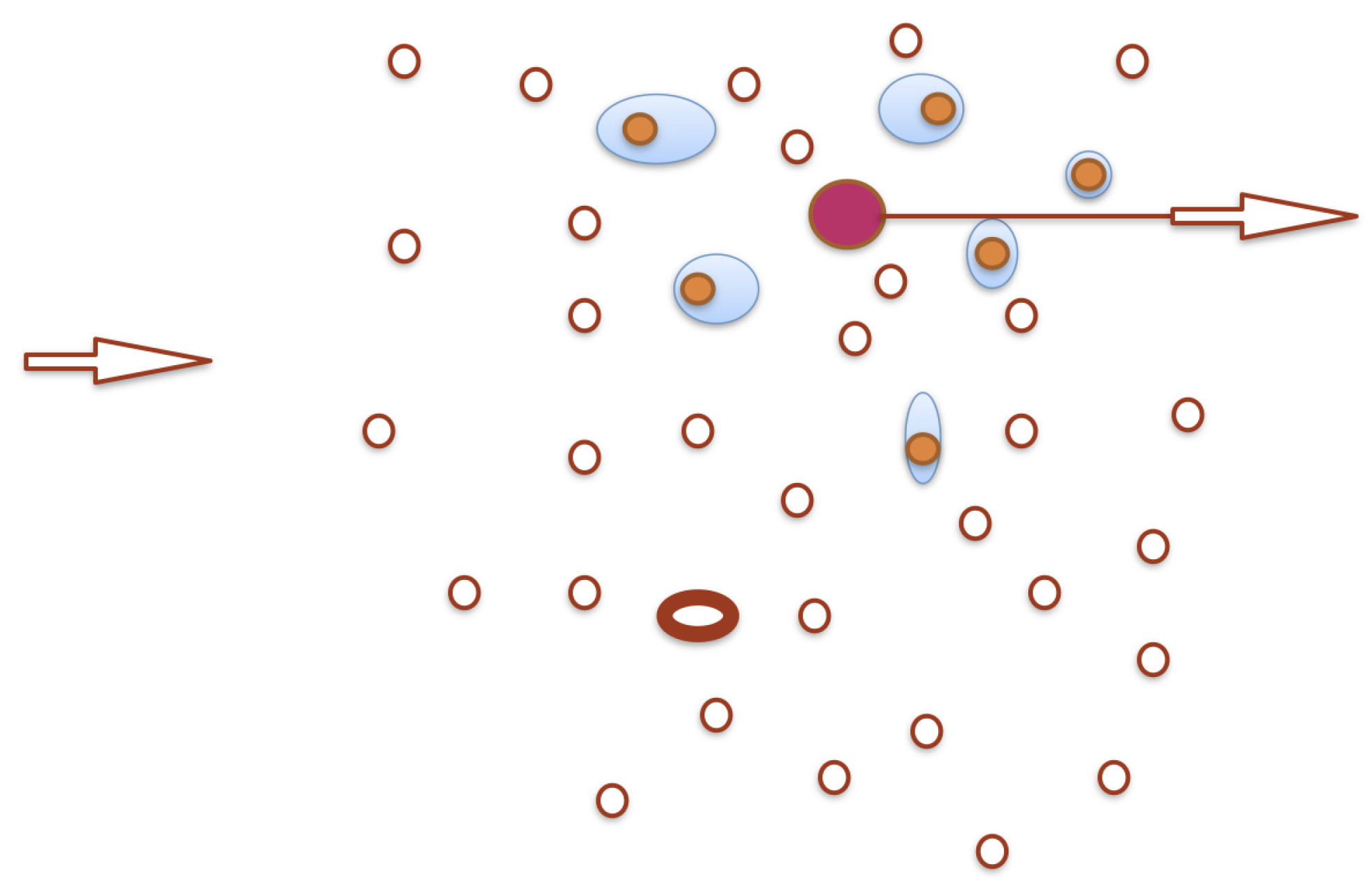
Intuitively, we can imagine a chatbot dialogic dynamics, within a Noematic Manifold $\mathcal{N}$, as a soccer pitch: The two teams are the interlocutors, and the state of a dialog, that is, the position of the semantic centroid after the last sentence, corresponds to the positions of the ball and the players at a given time (see Figure 1).

• The Noemes (embeddings) are the players, representing the available knowledge constants.
• The Centroid is the ball. The “kicks determine its position” (attentional weights) given by the players, but its trajectory depends on its previous position ($\sigma {\mathbf{C}}_{t-1}$).
• The Assertion (⊧) is a way to place the attention focus on the principal fact of a sentence. For this reason, the computation of attention coefficients uses a renormalization giving greater weights to the predicate of the asserted predication.

The centroid position encodes the meaning of the sentence received or produced by the chatbot. In the case of a received sentence, it is input to a text generation module for the right answer. Conversely, in the case of a produced sentence, it is the semantic reference for the answer that the chatbot will receive.

This architecture addresses the “Context Window” problem of current LLMs [2]. By using persistent identifiers ($a,b,c$), the Noematic Machine maintains deictic stability. Any subsequent reference to the constant a will target the same tensor coordinates in the register, regardless of the distance in the token stream, effectively creating a Logical Memory that is immune to probabilistic decay.

7.1. The Noematic Parser: Compiling Language into Tensor Streams

The transition from Natural Language to the Noematic Manifold ($\mathcal{N}$) is mediated by the Noematic Parser. This module acts as a compiler that transforms the linear sequence of tokens into a hierarchical Execution Graph based on FLL syntax.

7.1.1. Lexical Activation and Operator Triggering

As the sentence is processed, the parser identifies “Noematic Triggers” — lexical units that call specific FLL operators. The mapping follows a precise functional logic:

• Determiners and Proper Names: Invoke Op. 14 (Allocate) to stabilize a constant in the register file.
• Adverbs and Qualifiers: Invoke Op. 12 (Modify) to warp the target noeme through a $(1,1)$-tensor transformation.
• Prepositions (e.g., “by”, “with”): Invoke Op. 10 (Link) to establish hyperpredication and related tensor contraction.

7.1.2. The Wiring Map Generation

The parser does not merely list operators; it defines the logical schema for the attention mechanism. It produces a “Wiring Map” that dictates the sequence of tensor contractions. For a sentence such as “Giulio was quickly going home by his bike”, the parser generates a nested execution order: the “$By\_$” hypercomplementation (Link) ($T_{10}$), specification ($T_{11}$), and modification ($T_{12}$) must be resolved before the “Assertion” operator (⊧) can collapse the semantic centroid into its final state.

The following table (Table 2) defines the instruction set available to the Noematic Parser. Each FLL operator is mapped to its specific tensor class and the neural action it performs within the T-FLL Attention Cell. This dictionary serves as the “Instruction Set Architecture” of the “Noematic Machine”, providing the formal bridge between linguistic syntax and multilinear algebraic execution.

Table 2. T-FLL Operational Dictionary: From FLL to Tensor Execution.

#	FLL Operator	Tensor Class	Machine Instruction / Neural Act
1	$P\left(s\right)$	Contraction	Saturate: $P_i{\mathbf{s}}^i$ Predication
2	$s=E$	Indexicalization	Assign: ${\mathbf{v}}_s\leftarrow {\mathbf{v}}_E$ Constant Selection
3	$\widehat{P}$	Projection	Abstract: ${\mathbf{T}}_{i\widehat{P}}^j$ P-Implicability
4	$x.E\left(x\right)$	Cilindrification	Bind: ${\mathbf{T}}_j^i$ Functional Abstraction.
5	¬	Negation	Invert: ${\mathbf{R}}_j^i$ Orthogonal Inversion
6	$P\to Q$	Sum	Imply: Filonian Sum $\neg {\mathbf{T}}_P+{\mathbf{T}}_Q$
7	$P\wedge Q$	Sum	Intersect: Vector Sum ${\mathbf{T}}_P+{\mathbf{T}}_Q$
8	$P\vee Q$	Sum	Unite: Disjoint Sum $q{\mathbf{T}}_P+(1-q){\mathbf{T}}_Q$
9	$P\_s$	Contraction	Complement (direct): ${\mathbf{T}}_i^j{\mathbf{a}}_j$
10	$Prep\_s\left(P\right)$	Contraction	Link: ${\mathbf{T}}_i^j{\mathbf{a}}^j$ Relativization
11	$\langle s|$	Dualization	Specify: Vector ↦ Covector
12	$P\left[Q\right]$	Hadamard	Modify: ${\mathbf{T}}_P\odot {\mathbf{T}}_Q$ Noeme Warping
13	$\iota$	Unique Selection	Determinate: “The” Selection
14	$ϵ$	Stochastic Choice	Choose: “Any” Selection
15	⊧	Accumulation	Assert: Centroid Convergence
16	$?\vDash$	Potential Gap	Seek: Manifold Sink
17	$!\vDash$	Force Field	Drive: State Change
18	$(>1)\left[P\right]$	Summation	Cluster: Direct Sum $⨁{\mathbf{v}}_P$
19	$n\left[P\right]$	Numeration	Count: Dimension Rank
20	$n^{\circ }\left[P\right]$	Seriation	Order: Ordinal Ranking

Table 2. T-FLL Operational Dictionary: From FLL to Tensor Execution.

#	FLL Operator	Tensor Class	Machine Instruction / Neural Act
1	$P\left(s\right)$	Contraction	Saturate: $P_i{\mathbf{s}}^i$ Predication
2	$s=E$	Indexicalization	Assign: ${\mathbf{v}}_s\leftarrow {\mathbf{v}}_E$ Constant Selection
3	$\widehat{P}$	Projection	Abstract: ${\mathbf{T}}_{i\widehat{P}}^j$ P-Implicability
4	$x.E\left(x\right)$	Cilindrification	Bind: ${\mathbf{T}}_j^i$ Functional Abstraction.
5	¬	Negation	Invert: ${\mathbf{R}}_j^i$ Orthogonal Inversion
6	$P\to Q$	Sum	Imply: Filonian Sum $\neg {\mathbf{T}}_P+{\mathbf{T}}_Q$
7	$P\wedge Q$	Sum	Intersect: Vector Sum ${\mathbf{T}}_P+{\mathbf{T}}_Q$
8	$P\vee Q$	Sum	Unite: Disjoint Sum $q{\mathbf{T}}_P+(1-q){\mathbf{T}}_Q$
9	$P\_s$	Contraction	Complement (direct): ${\mathbf{T}}_i^j{\mathbf{a}}_j$
10	$Prep\_s\left(P\right)$	Contraction	Link: ${\mathbf{T}}_i^j{\mathbf{a}}^j$ Relativization
11	$\langle s|$	Dualization	Specify: Vector ↦ Covector
12	$P\left[Q\right]$	Hadamard	Modify: ${\mathbf{T}}_P\odot {\mathbf{T}}_Q$ Noeme Warping
13	$\iota$	Unique Selection	Determinate: “The” Selection
14	$ϵ$	Stochastic Choice	Choose: “Any” Selection
15	⊧	Accumulation	Assert: Centroid Convergence
16	$?\vDash$	Potential Gap	Seek: Manifold Sink
17	$!\vDash$	Force Field	Drive: State Change
18	$(>1)\left[P\right]$	Summation	Cluster: Direct Sum $⨁{\mathbf{v}}_P$
19	$n\left[P\right]$	Numeration	Count: Dimension Rank
20	$n^{\circ }\left[P\right]$	Seriation	Order: Ordinal Ranking

8. Relevance of T-FLL Representation for Transformers

The integration of T-FLL into the Transformer architecture addresses three critical bottlenecks in current AI development: hallucinations, lack of explainability, and long-range coherence.

8.1. Mitigating Hallucinations Through Structural Constraints

Standard LLMs often generate factually incorrect but syntactically plausible strings because their internal representations lack a formal grounding. In T-FLL, every predication must satisfy a threshold of noematic adherence $\theta$. By forcing the Attention mechanism to respect the FLL operator logic (e.g., ensuring that the hypercomplementation $With\_a\left(P\right)$ maintains the correct tensor rank), we impose a “logical filter” that prevents the system from merging incompatible semantic regions.

8.2. Explainable Reasoning and Traceability

The Semantic Centroid $\mathbf{C}$ serves as a mathematical proof of the system’s reasoning path. Unlike the “black box” nature of current hidden states, a T-FLL centroid can be decomposed into its original noematic components ($T_k$) and their respective weights (${\alpha }_k$). Researchers can inspect whether a model’s failure was due to an incorrect noematic abstraction or a misalignment in the determination operator ($\iota$).

Current models struggle with long-term anaphora because positional encodings and attention masks are finite. T-FLL introduces persistent semantic registers through constants. By mapping these to fixed tensor indices that do not decay over time, the system can maintain the identity of an individual a across thousands of tokens, transforming the chatbot into a system with a structured and enduring internal model of the world.

9. Conclusions

The integration of FLL into the tensor-based architecture of modern AI models represents more than a technical optimization; it is a return to the foundational dream of a characteristica universalis. By formalizing the “Noematic Space” as a differentiable manifold governed by precise functional operators, we have outlined a framework where meaning is a geometric necessity.

T-FLL effectively bridges the gap between the intuitive, flexible nature of human language and the rigorous, verifiable nature of formal logic. As we move toward more autonomous and critical AI systems, the ability to anchor neural weights to formal logical structures like the FLL Semantic Centroid will be the deciding factor in creating machines that do not just simulate understanding but operate within a coherent and explainable model of reality.

The transition from a purely distributional model of language to a functional-tensor framework marks a significant shift in computational linguistics. By mapping the 20 operators of Functional Language Logic (FLL) onto the multi-linear algebra of Transformers, we have suggested that semantic coherence can be formally governed rather than statistically estimated.

T-FLL provides a rigorous solution to the problem of reference stability through constant registers and offers a transparent mechanism for semantic convergence via the Semantic Centroid. This integration represents more than a technical optimization; it shows the link between the logical structure of meaning (FLL noematic formulae) to its geometric perspective (embedding vectors). Namely, the noematic space is a differentiable manifold governed by precise functional operators, where meaning emerges as a geometric necessity.

As we move toward more autonomous and critical AI systems, the ability to anchor neural weights to formal logical structures –like the FLL Semantic Centroid– will be the deciding factor in creating machines that do not just simulate understanding through “probabilistic parrots”, but operate within a coherent, explainable, and structurally grounded model of reality. Future research will focus on the empirical implementation of these tensor constraints within the training objectives of neural architectures, aiming for a truly synthetic intelligence that inhabits the geometry of thought.

References

- Bahdanau, D.; Cho, K.; Bengio, Y. Neural Machine Translation by Jointly Learning to Align and Translate. arXiv 2014, arXiv:1409.0473. [Google Scholar]
- Beltagy, l.; Peters, M.E.; Cohan, A. Longformer: The Long-Document Transformer. arXiv [cs.CL]. 2020, arXiv:2004.05150. [Google Scholar] [CrossRef]
- Goodfellow, I.; Bengio, Y.; Courville, A. Deep Learning; MIT Press, 2016. [Google Scholar]
- Bishop, R. L.; Goldberg, S. I. Tensor Analysis on Manifolds; Dover Publications, 1980. [Google Scholar]
- Church, A. : A formulation of the simple theory of types. Journal of Symbolic Logic 1940, 5(2), 56–68. [Google Scholar] [CrossRef]
- Church, A. Introduction to Mathematical Logic; Princeton University Press, 1956. [Google Scholar]
- Coelho, F.; Martins, B. “On the Geometry of Word Embeddings,” In Proceedings of the 2021 EMNLP (2021).
- Cybenko, G. : Approximation by superpositions of a sigmoidal function. Mathematics of Control, Signals, and Systems 1989, 2(4), 303–314. [Google Scholar] [CrossRef]
- Dziri, N. Faith and Fate: Limits of Transformers on Compositionality, Advances in Neural Information Processing Systems, 36 (NeurIPS 2023), Ernest N. Morial Convention Center, New Orleans (LA), USA, 10-16 (2023).
- Hilbert, D.; Ackermann, W. Principles of Mathematical Logic (tr. from German, 1928); AMS Chelsea Publishing, 1991. [Google Scholar]
- Hinton, G. E. Implementing semantic networks in parallel hardware. In Parallel Models of Associative Memory; Hinton, G. E., Anderson, J.A., eds.; Lawrence Erlbaum Associates., 191–217 (1981), available online: https:taylorfrancis.com/chapters/edit/10.4324/9781315807997-13/implementing-semantic-networks-parallel-hardware-geoffrey-hinton (accessed on 1 December 2024).
- Hopfield, J. J. Neural networks and physical systems with emergent collective computational abilities. Proc. Natl. Acad. Sci. USA 1982, 79, 2554–2558. [Google Scholar] [CrossRef] [PubMed]
- Hornick, K.; Stinchcombe, M.; White, M. Multilayer feedforward networks are universal approximators. Neural Networks 1989, 2, 359–366. [Google Scholar] [CrossRef]
- Kaplan, J. et al., Scaling Laws for Neural Language Models. arXiv 2020, arXiv:2001.08361. [Google Scholar] [CrossRef]
- Une Procédure d’Apprentissage pour Réseau à Seuil Asymétrique. In Cognitiva 85: À la Frontière de l’Intelligence Artificielle des Sciences de la Connaissance des Neurosciences, Proceedings of Cognitiva 85, Paris, France, 1985; 599–604. (1985) Available online: https://www.academia.edu (accessed on 1 December 2024).
- Lovett, S. Differential Geometry of Manifolds; A K Peters/CRC Press, 2010. [Google Scholar]
- Manca, V.: A Metagrammatical Logical Formalism, in C. Martín-Vide (ed.), Mathematical and Computational Analysis of Natural Language, John Benjamins (1998).
- Manca, V.: Formal Logic. In: J. G. Webster (ed.), Encyclopedia of Electrical and Electronics Eng., John Wiley & Sons, 7, 675-687 (1999).
- Manca, V. Agile Logical Semantics for Natural Languages. Information MDPI 2024, 15(1), 64. [Google Scholar] [CrossRef]
- Manca, V. On the functional nature of cognitive systems. Information MDPI 2024, 15(12), 807. [Google Scholar] [CrossRef]
- Manca, V. Functional Language Logic. Electronics MDPI 2025, 14(3), 460. [Google Scholar] [CrossRef]
- Manca, V. : Knowledge and Information in Epistemic Dynamics. www.preprints.org, 17 October 2025 2025. [Google Scholar] [CrossRef]
- Mikolov, T.; Sutskever, I.; Chen, K.; Corrado, G.; Dean, J. Distributed Representations of Words and Phrases and their Compositionality. arXiv [cs.CL]. 2013, arXiv:1310.4546. [Google Scholar] [CrossRef]
- Minsky, M. Computation. Finite and Infinite Machines; Prentice-Hall Inc.: Upper Saddle River, NJ, USA, 1967. [Google Scholar]
- Mitchell, T. Machine Learning; McGraw Hill, 1997. [Google Scholar]
- Montague, R.: English as a formal language, In B. Visentini et al. (eds) I Linguaggi nella Società e nella Tecnica, Milan (1970).
- Montague, R. : Universal Grammar. Theoria 1970, 36, 373–398. [Google Scholar] [CrossRef]
- Montague, R.: The Proper Treatment of Quantification in Ordinary English, https://www.cs.rhul.ac.uk/ zhaohui/montague73.pdf (1973).
- Nielsen, M. Neural Networks and Deep Learning Online. 2013.
- OpenAI, GPT4-Technical Report, ArXiv: submit/4812508 [cs.CL]. 27 Mar 2023.
- Oudeyer, P-Y; Kaplan, F.; Hafner, V. Intrinsic Motivation Systems for Autonomous Mental Development . IEEE Transactions on Evolutionary Computation 2007, 11(2), 265–286. [Google Scholar] [CrossRef]
- Parkinson, G. R.: Leibniz Logical Papers; Clarendon Press, 1966. [Google Scholar]
- Peano, G. Opere Scelte, vol. II: Logica Matematica. Interlingua ed Algebra della Grammatica, Edizioni Cremonese (1958).
- Chen, L.; Peng, B.; Wu, O. Theoretical limitations of multi-layer Transformer. arXiv [cs.LG]. 2024, arXiv:2412.02975. [Google Scholar] [CrossRef]
- Reichenbach, H. Elements of Symbolic Logic; MacMillan, 1947. [Google Scholar]
- Rosenblatt, F. The perceptron: A probabilistic model for information storage and organization in the brain. Psychol. Rev. 1958, 65, 386–408. [Google Scholar] [CrossRef] [PubMed]
- Rumelhart, D.; Hinton, G.; Williams, R. Learning representations by back-propagating errors. Nature 1986, 323, 533–536. [Google Scholar] [CrossRef]
- Smolensky, P. Tensor product variable binding and the representation of symbolic structures in connectionist systems. Artificial Intelligence 1990, 46(1-2), 159–216. [Google Scholar] [CrossRef]
- Vaswani, A. et al., “Attention is All You Need. In Advances in Neural Information Processing Systems (NIPS); 2017. [Google Scholar]
- Zach, R. The Practice of Finitism: Epsilon Calculus and Consistency Proofs in Hilbert’s Program. arXiv [math.LO]. 2001, arXiv:math/0102189. [Google Scholar] [CrossRef]
Figure 1.
An image of a dialogic game: The circles scattered are the noemes located in the semantic space. The left arrow is the input text T, which activates the noemes belonging to the text. The forms surrounding the activated noemes represent the attention weights constrained by the FLL Wiring Map. The colored circle represents the Semantic Centroid , the point of convergence within the manifold that serves as the basis for the generation of the response to the input text T. The bold line oval represents the previous centroid
Disclaimer/Publisher’s Note: The statements, opinions and data contained in all publications are solely those of the individual author(s) and contributor(s) and not of MDPI and/or the editor(s). MDPI and/or the editor(s) disclaim responsibility for any injury to people or property resulting from any ideas, methods, instructions or products referred to in the content. |
© 2026 by the authors. Licensee MDPI, Basel, Switzerland. This article is an open access article distributed under the terms and conditions of the Creative Commons Attribution (CC BY) license (http://creativecommons.org/licenses/by/4.0/).
Copyright: This open access article is published under a Creative Commons CC BY 4.0 license, which permit the free download, distribution, and reuse, provided that the author and preprint are cited in any reuse.