

Submitted:
28 May 2024
Posted:
29 May 2024
You are already at the latest version
Abstract
We leverage the explainability feature of KAN network and build an explainable language model where certain neurons encode individual words and neuron activation is fully interpretable in terms of the basis of a word. To do that, we propose a continuous word2vec model where a meaning of a word is expressed by a continuous profile of distances of this word from the words in the basis of words which is interpolated. As a result, the whole KAN network can be interpreted as a sequential procedure with word expressions. We then proceed from words to logic programs and develop a clause learning technique based on KAN. A logic program construction process from facts now become fully interpretable. We follow the differentiable inductive logic programming technique, representing a logic program as a matrix learned by KAN. Hence, we obtain an efficient and fully interpretable rule learning approach.
Keywords:
Kolmogorov-Arnold network
; explainability
; symbolic regression
; continuous word2vec model
; inductive logic programming
1. Introduction
Inspired by the Kolmogorov-Arnold representation theorem, (Liu et al 2024) propose Kolmogorov-Arnold Networks (KANs) as promising alternatives to Multi-Layer Perceptrons (MLPs). KAN is a fresh perspective on Neural Networks, a cornerstone of current machine learning (ML). In ML, the ability to efficiently and accurately approximate complex functions is an important subject, especially as the dimensionality of data increases. The Kolmogorov-Arnold theorem, however, provides a theoretical foundation for building networks (like KANs) that can overcome this challenge.
The Kolmogorov-Arnold representation theorem is a significant result in the field of mathematics, particularly in the theory of functions. It asserts that any multivariate continuous function can be represented as a finite sum of continuous univariate functions. The theorem shows that any function of multiple variables can be decomposed into a sum of functions of single variables. This theorem implies that multivariate functions can be broken down into simpler, univariate components. This decomposition can simplify the analysis and computation of complex functions. While the theorem is theoretically powerful, its practical application can be limited due to the potential complexity of the resulting univariate functions. These functions may not be easily learnable or approximable by simple models, which poses challenges in fields like machine learning.
While MLPs have fixed activation functions on nodes (“neurons”), KANs have learnable activation functions on edges (“weights”). KANs have no linear weights at all – every weight parameter is replaced by a univariate function parametrized as a spline (Igelnik and Parikh 2003). This architectural update makes KANs outperform MLPs in terms of accuracy and interpretability. For accuracy, much smaller KANs can achieve comparable or better accuracy than much larger MLPs in data fitting and Partial Differential Equation solving. Theoretically and empirically, KANs possess faster neural scaling laws than MLPs. For interpretability, KANs can be intuitively visualized and can easily interact with human users. KANs can “collaborate” with scientists in discovering mathematical and physical phenomenology. Hence, KANs are promising alternatives for MLPs, opening opportunities for further improving Transformer architecture which leverages MLPs today.
We aim to leverage the interpretability of KAN to support inductive learning. Inductive Logic Programming (ILP) comprises techniques for constructing logic programs from examples. Given a set of positive examples and a set of negative examples, an ILP system constructs a logic program that entails all the positive examples while excluding the negative ones. From a machine learning perspective, an ILP system acts as a rule-based binary classifier, mapping each example to a truth or falsehood evaluation based on the provided axioms and newly inferred rules during training.
Neuro-symbolic ILP is rapidly emerging as a crucial research domain in inductive synthesis (Cropper and Dumancic 2022). These systems enhance explainability research by offering logical representations of learned information and providing noise-handling capabilities for symbolic learners. Systems like δILP consistently learn solutions for many standard inductive synthesis problems (Evans and Grefenstette 2018).
Synthesizing large logic programs through symbolic ILP typically requires intermediate definitions. However, introducing invented predicates can clutter the hypothesis space and degrade performance. In contrast, gradient descent efficiently finds solutions within high-dimensional spaces, a property not fully utilized by neuro-symbolic ILP approaches. Purgal et al. (2023) propose extending the differentiable ILP framework with large-scale predicate invention, exploiting the efficiency of gradient descent. This large-scale predicate invention benefits differentiable inductive synthesis, leading to learning capabilities beyond existing neuro-symbolic ILP systems.
To build language model and make KAN interpretable performing NLP tasks, we generalize word2vec model towards continuous profiles which can by a subject of a regression performed by KAN.
The Value of Interpretability
While neural networks such as MLPs have achieved state-of-the-art performance on benchmark datasets and real-world applications, they function as black-box systems, unable to explain their predictions in a manner understandable to humans. A common approach to mitigate the issues of black-box models is to construct a secondary (post-hoc) model to explain the original model, such as SHAP (Lundberg and Lee 2017) or LIME (Ribeiro et al. 2017). However, there is a popular opinion that post-hoc explanations are inherently flawed (Rudin 2019). Post-hoc explanations cannot achieve perfect fidelity with respect to the original model. If the explanation were entirely faithful to the original model, it would essentially replicate the original model itself, rendering the original model redundant.
Additionally, label noise is a prevalent issue in datasets. It has been reported that real-world datasets typically contain 10-40% label noise. There is theoretical evidence suggesting that in noisy datasets, such as those found in healthcare, simple, interpretable classifiers can perform as well as black-box models (Semenova et al. 2024).
If a neural network architecture can reproduce the structure of a domain and also support interaction with a human expert during the training session, that would be an essential step towards explainability of a prediction. If each layer of a network can be interpreted in terms of the original stimuli, such as a phrase or an image fragment, it would significantly enhance the interpretability of the solution. Developing explainability features based on KAN architecture is a promising direction, leveraging the flexibility of individual KAN neurons. Once an ML engineer can prune the network to adjust it to a particular problem domain, this joint man-machine development can further advance network interpretability. In this chapter, we will develop machinery to make textual prediction explainable, following the symbolic regression task of KAN (Liu et al. 2024).
Combining inherently explainable logic programming with KAN is a further step towards interpretability and joint man-machine activity in deriving and operating with rules from data. Differentiable Inductive Logic Programming turns out to be a feasible formalism for integration with KAN, both possessing explainability features.
2. KAN Architecture
KAN and Multi Layered Perceptron
If f is a multivariate continuous function on a bounded domain, then f can be written as a finite composition of continuous functions of a single variable and the binary operation of addition. More specifically, for a smooth f: [0,1]n 0
The outer function fis represented as a finite sum of transformed univariate functions. These univariate functions, φ(q,p) can be highly complex, non-smooth, and even fractal-like. This complexity can pose significant challenges for the practical application of the theorem.
The only genuinely multivariate function is addition, as every other function can be expressed using univariate functions and summation. At first glance, this might seem like great news for machine learning: learning a high-dimensional function could be reduced to learning a polynomial number of 1D functions. However, these 1D functions can be non-smooth and even fractal, making them potentially unlearnable in practice (Fakhoury et al. 2022). Due to this pathological behavior, the ML community remained pessimistic about the practical applications of the Kolmogorov-Arnold representation theorem.
At the same time, MLP is based on Universal Approximation Theorem where an arbitrary function f(x) is represented as
It states that a feedforward neural network with a single hidden layer containing a finite number of neurons can approximate any continuous function on a compact subset of Rn, given appropriate weights and activation functions. Essentially, this means that neural networks can represent a wide variety of functions to any desired degree of accuracy, under certain conditions. Even a neural network with just one hidden layer (a single-layer feedforward network) can approximate any continuous function, provided the hidden layer has a sufficient number of neurons. The choice of activation function is crucial; common functions that satisfy the theorem include the sigmoid function, hyperbolic tangent (tanh), and rectified linear unit (ReLU). The accuracy of the approximation depends on the number of neurons in the hidden layer. Generally, more neurons lead to better approximation, but the exact number required depends on the complexity of the target function.
While MLPs place fixed activation functions on nodes (“neurons”), KANs place learnable activation functions on edges (“weights”). As a result, KANs have no linear weight matrices at all: instead, each weight parameter is replaced by a learnable 1D function parametrized as a spline. KANs’ nodes simply sum incoming signals without applying any non-linearities.
In spite of their elegant mathematical foundation, KANs (Kolmogorov-Arnold Networks) are essentially combinations of splines and MLPs (Multilayer Perceptrons), capitalizing on their respective strengths while mitigating their weaknesses. Splines excel at handling low-dimensional functions, are easy to adjust locally, and can switch between different resolutions. However, they suffer from the curse of dimensionality (COD) due to their inability to exploit compositional structures. On the other hand, MLPs are less affected by COD thanks to their feature learning capabilities but are less accurate than splines in low-dimensional settings because they cannot optimize univariate functions as effectively. For a model to accurately learn a function, it must capture the compositional structure (external degrees of freedom) and approximate univariate functions well (internal degrees of freedom). KANs achieve this balance by integrating MLPs on the outside and splines on the inside.
KAN Architecture
The architecture of Kolmogorov-Arnold Networks (KANs) revolves around a novel concept where traditional weight parameters are replaced by univariate function parameters on the edges of the network. Each node in a KAN sums up these function outputs without applying any nonlinear transformations, in contrast with MLPs that include linear transformations followed by nonlinear activation functions.
A general KAN network is a composition of L layers (Figure 2): given an input vector x0 ∈ , the output of KAN is
KAN(x) = (ΦL−1 ◦ Φ L−2 ◦ °… ◦ Φ1 ◦ Φ0)x.
Notice that an MLP can be written as interleaving of affine transformations
where Wn are linear weight parameters and is a nonlinear activation function
MLP(x) = WL-1 ◦ σ◦ WL-2 ◦ σ◦… ◦ Φ1 ◦σ ◦Φ0)x,
(Liu et al. 2024) extend the network (*) to accommodate arbitrary widths and depths. Most functions in science and engineering are often smooth and exhibit sparse compositional structures, which can enable smooth Kolmogorov-Arnold representations. This approach aligns with the mindset of physicists, who typically focus on typical cases rather than worst-case scenarios. Ultimately, both our physical world and machine learning tasks must possess inherent structures to make physics and machine learning useful and generalizable.
An example of activation for is shown in Figure 3.
KAN layer with nin-dimensional inputs and nout-dimensional outputs can be defined as a matrix of 1D function
where the functions have trainable parameters. In the Kolmogov-Arnold theorem, the inner functions form a KAN layer with nin = n and nout = 2n+1, and the outer functions form a KAN layer with nin = 2n + 1 and nout = 1.
Regularization and Activation Functions in KANs
KANs’ linear weights are replaced by learnable activation functions, so one should define the L1 norm of these activation functions. For MLPs, L1 regularization of linear weights is used to favor sparsity.
L1 regularization is a technique used in ML, particularly in linear models like linear regression or linear classifiers such as logistic regression. It is used to prevent overfitting and to encourage simpler models by penalizing the absolute magnitude of the coefficients (weights) in the model. In the context of linear models, the L1 regularization adds a penalty term to the loss function proportional to the absolute value of the coefficients. This penalty is often represented by the L1 norm of the weight vector. When the optimization algorithm minimizes this penalized loss function, it tends to drive many of the coefficients towards zero.
The effect of this regularization is to encourage sparsity in the solution, meaning that many of the coefficients become exactly zero. In other words, L1 regularization tends to drive irrelevant or less important features to have zero coefficients, effectively removing them from the model. This is particularly useful when dealing with high-dimensional data where many features may not contribute significantly to the predictive power of the model.
Activation functions introduce non-linearity into neural networks, allowing them to model complex relationships between inputs and outputs. In NLP tasks, activation functions are typically applied at each neuron in the neural network layers, including input, hidden, and output layers. Popular activation functions for MLP include ReLU (Rectified Linear Unit), sigmoid, and tanh.
In NLP networks, the activation function of a neural network does not directly encode the meaning of a sentence. Instead, it serves to introduce non-linearity into the network, enabling it to learn complex relationships between inputs and outputs. However, the activations across the network layers, combined with the parameters (weights and biases), collectively contribute to the model’s ability to understand and represent the meaning of sentences.
The selection of activation functions in a neural network has a significant impact on the training process. There is, however, no obvious way to choose them because the “optimal choice” may depend on the specific task or problem to be solved. Nowadays, ReLU activation functions (and variations) are the default choice in the broad spectrum of activation functions for many types of neural networks.
In NLP, the input to a neural network representing a sentence is typically a sequence of word embeddings. Each word embedding captures some information about the meaning of the word it represents. As the input passes through the network, activations in different layers encode increasingly abstract representations of the input sentence. At each layer, the activation function (e.g., ReLU, sigmoid) transforms the weighted sum of inputs into an output signal.
Neural networks, particularly those used in NLP tasks like sentence classification or sentiment analysis, are capable of learning compositional representations. This means that they can understand the meaning of a sentence by combining the meanings of its constituent words and phrases. The activation patterns in the network layers capture these compositional relationships. During the training process, the MLP network adjusts its parameters (weights and biases) based on the input-output pairs provided in the training data. The activation function plays a crucial role in determining how the network learns to map input representations to output predictions. Through backpropagation and gradient descent, the network learns to adjust its parameters to minimize the loss function, thereby improving its ability to capture the meaning of sentences.
While the activation function itself does not encode the meaning of a text, it contributes to the overall capability of the neural network to learn and represent semantic information. The meaning of a sentence emerges from the collective behavior of the network’s activations and parameters, shaped by the training data and the task-specific objective.
Activation functions of KAN are designed as follows:
Residual activation function include a basis function b(x) (similar to residual connections) such that the activation function ϕ(x) is the sum of the basis function b(x) and the spline function:
ϕ(x) = w (b(x) + spline(x))
b(x) = SiLU(x) = x/(1 + e-x)
The SiLU activation function can be seen as a smooth version of the ReLU (Rectified Linear Unit) activation function. It maintains all the desirable properties of ReLU, such as sparsity and non-saturation of gradients, while also being smooth and differentiable everywhere. This smoothness can help with gradient-based optimization methods during training.
Compared to ReLU, which can sometimes suffer from a “dying ReLU” problem where neurons can become inactive during training and never recover, SiLU tends to have a more consistent gradient flow throughout the network, potentially leading to better convergence and performance.
spline(x) is parametrized as a linear combination of B-splines such that
spline(x) = where ci-s are trainable. w is not essential it can be absorbed into b(x) and
spline(x). Each activation function is initialized to have spline(x) ≈ 0.
B-Splines
Univariate spline functions are a valuable tool in approximation theory (Lyche et al. 2018). These functions are piecewise polynomials with a specific degree and global smoothness. Notably, maximally smooth splines exhibit exceptional approximation behavior relative to the degree of freedom (Sande et al. 2019). ReLU functions can be considered linear spline functions. More flexible (learnable) spline activation functions, as studied by Bohra et al. (2020), have shown that their adaptability can reduce the overall network size required to achieve a given accuracy. Therefore, there is a trade-off between the complexity of the network architecture and the complexity of the activation functions.
Univariate spline functions can be expressed as linear combinations of B-splines, a set of locally supported basis functions that form a nonnegative partition of unity. B-spline representations are ideal for approximating univariate smooth functions because they can be compactly described by a small number of parameters, with each parameter having a local effect. Efficient algorithms for their computation are available (Lyche et al. 2018). Multivariate extensions can be readily achieved by taking tensor products of B-splines (Figure 4).
Definition of B-splines necessitates the concept of knot sequence. A knot sequence is a nondecreasing
sequence of real numbers,
:= { 1 2 … r }. The elements of are called knots. Assuming integer values r p + 2 2, on such sequence it is possible to define N := r - p - 1 B-splines of degree p:
Given a knot sequence , the n-th B-spline of degree p 0 is zero if n+p+1 = n
and otherwise defined recursively by
The multivariate B-spline vector can be interpreted as a fuzzy hierarchical partition of the domain that induces a tree structure with L levels for every t = 1, …, T. This can be explained as follows. Let us fix t. For each l = 1, . . . , L, by construction, () is a vector of B-splines of degree . Its components are nonnegative real values that sum up to one, and thus can be regarded as a distribution over a discrete set of hidden classes {} at level l, where for = 1, . . . , we have
The B-spline plays the role of decision or gating function at level l based on the feature x). Then, under the assumption that the events are mutually independent, the joint probability on the hierarchy of hidden classes at all levels is given by
for = 1, . . . , and l = 1, . . . , L. All together they form the multivariate B-spline vector. A graphical representation of the induced tree structure is in Figure 5.
Symbolic Regression in KAN
What is a good way to select KAN shape that best reflects the structure of a dataset?
For instance, if we know the dataset is generated via the symbolic formula f(x,y)=exp(sin(πx)+y2), then it is obvious that a [2, 1, 1] KAN can “implement” this function. In real-world scenarios, however, an ML designer usually doesn’t have this information in advance, so it’s beneficial to determine the KAN shape automatically. The strategy involves starting with a sufficiently large KAN and training it with sparsity regularization followed by pruning. These pruned KANs turn out to be much more interpretable than their non-pruned counterparts. To further enhance interpretability, Liu et al. (2024) propose several simplification techniques and provide examples of how users can interact with KANs to make them more interpretable.
In cases where the activation functions turn out to be symbolic (e.g., tanh or sin), there is an interface to set them to be a specified symbolic form, fix_symbolic(l,i,j,f) that sets the (l, i, j) activation to be f. However, one cannot just convert the activation function into be the exact symbolic formula, since its inputs and outputs may have shifts and scaling. Therefore, pre-activations x and post-activations y needs to be computed from training data, and needs to fit affine parameters (a, b, c, d) such that y ≈ c f(ax+b)+d. The fitting is done by iterative grid search of a, b and linear regression (Figure 7).
The symbolic space is densely filled, making it challenging to derive the correct symbolic formula. In some cases, such a formula might not exist at all. KAN can maintain the sensitivity of symbolic regression, especially in the presence of noise, which has its pros and cons. Fortunately, it is relatively easy to identify symbolic formulas that closely align with the data, often within an acceptable margin of error (epsilon). While these approximate symbolic formulas may not precisely capture the underlying relationship, they still offer valuable insights, possess predictive capabilities, and are computationally efficient.
The limitation of KAN is that determining the exact formula proves to be a formidable challenge. This becomes crucial in scenarios where precision is paramount, either for generalizability in tasks in physics or for fitting experimental data or solving partial differential equations with machine-like accuracy. For the former scenario, the quest for generalizability is ongoing and requires meticulous examination on a case-by-case basis. In the latter case, we can gauge the fidelity of a symbolic formula by observing a reduction in loss approaching machine precision.
User Interacting with Explainable KAN
Neural networks, with their intricate structures and multitude of parameters, often pose challenges in understanding the inner workings of their resulting functions. This complexity has earned them the moniker of „black-box models,” as their behavior can be highly unpredictable, particularly in contexts where comprehending the rationale behind a decision is crucial. To address this, specific assumptions tailored to the task at hand can be imposed on the neural network’s architecture, such as utilizing convolutional neural networks for image-related tasks. Additionally, post-hoc gradient-based methods, as suggested by Ribeiro et al. (2016), can be employed to unravel the contributions of features to the final decision.
Alternatively, simpler models like linear and additive models, as proposed by Hastie and Tibshirani (1990), offer an avenue to circumvent the challenges posed by neural networks. Additive models, inspired by KAN tree models, offer high interpretability by basing predictions on a hierarchical partition of the input space, represented as a list of rules. In contrast, classical decision trees are susceptible to overfitting due to their piecewise constant nature and the inherent instability introduced by the greedy algorithms used in their learning process. Probabilistic or fuzzy trees, however, exhibit greater resilience to noisy data and are adept at handling uncertainty in imprecise contexts and domains. Performance can be further enhanced through ensemble techniques such as random forests. Various neural network architectures have been devised to mimic the interpretability of additive models, as demonstrated by Potts (1999), and to emulate classical or fuzzy tree structures, as explored by Kontschieder et al. (2015).
Explainability in KAN is implemented as a result of network simplification.
Simplification choices can be viewed as a hypothetical seizers a user can cut a network node. A user interacting with the network can select which node is most promising to cut next to make KANs more interpretable.
Let us consider the regression task f(x, y) = exp(sin(πx)+y2) example. Given data points (xi, yi, fi), i = 1, 2,…, Np, a user attempts to derive a symbolic formula. The steps of user interaction with the KANs are as follows:
(1) Training with making the network more sparse. Starting from a fully-connected [2, 5, 1] KAN, training with
regularization can make the network significantly more sparse. Four out of five neurons in the hidden layer turn out to not perform any function and can be removed.
(2) Network reduction. Automatic pruning is seen to discard all hidden neurons except the last one,
leaving a [2, 1, 1] KAN. The activation functions appear to be known symbolic functions.
(3) Setting symbolic functions. Assuming that the user can correctly guess these symbolic
formulas from staring at the KAN plot, she can set
fix_symbolic(0,0,0,‘sin’)
fix_symbolic(0,1,0,‘xˆ2’)
fix_symbolic(1,0,0,‘exp’).
In case the user has no domain knowledge or no idea which symbolic functions these activation
functions might be, there is a function suggest_symbolic to suggest symbolic candidates.
(4) Perform more training. After turning all the activation functions in KAN into symbolic form, the only remaining parameters are the affine parameters. These affine parameters require additional training. Once the loss is minimized, the corresponding symbolic expression is expeted to be correct.
(5) Produce a symbolic formula of the output node. The user obtains 1.0e1.0y2+1.0sin(3.14x), which is the true answer. For compactness, only two decimals for π are shown.
Making Neural network more sparse refers to the process of reducing the number of parameters (weights and biases) in a neural network while attempting to maintain its performance. This is done by setting a significant number of the network’s weights to zero, effectively making the network “sparse.” Sparsification can lead to several benefits, including reduced computational complexity, lower memory usage, faster inference times, and potentially improved generalization. There are several techniques for making KAN more sparse (Figure 8):
- (1)
- Pruning: This involves removing weights that contribute the least to the overall performance of the network. Pruning can be done based on magnitude (removing weights with the smallest absolute values), sensitivity (removing weights that cause the least change in the loss function), or structured pruning (removing entire neurons, filters, or channels).
- (2)
- Regularization: Techniques like L1 regularization can encourage sparsity by adding a penalty to the loss function that is proportional to the sum of the absolute values of the weights. This encourages many weights to become exactly zero during training.
- (3)
- Quantization: This process reduces the precision of the weights, which can lead to many weights effectively becoming zero, contributing to sparsity.
- (4)
- Low-rank factorization: This technique approximates the weight matrices in the network by lower-rank matrices, which can lead to a sparser representation.
- (5)
- Sparse training: Training algorithms can be modified to enforce sparsity directly during the training process. Techniques such as DropConnect randomly drop connections during training, which can lead to a sparser network (Wan et al 2013).
The main goal of making neural network more sparse is to create a more efficient model that retains as much of the original performance as possible while reducing resource requirements. Making neural network more sparse is particularly valuable for deploying neural networks on devices with limited computational power and memory, such as mobile phones or embedded systems.
3. KAN for Explainable NLP
Continuous word2vec
Representing the meaning of a word by a continuous function is a fundamental concept in NLP known as word embedding. Word embeddings are dense vector representations of words in a vector space, where each dimension of the vector captures different aspects of the word’s meaning.
One popular method for generating word embeddings is Word2Vec, which is based on the distributional hypothesis: words that appear in similar contexts tend to have similar meanings. Word2Vec learns word embeddings by training a neural network model to predict the context words given a target word (continuous bag of words) or predict the target word given context words (skip-gram) from a large corpus of text. Once trained, the hidden layer of the neural network serves as the word embeddings. These embeddings can then be used to represent the meaning of words in downstream NLP tasks such as sentiment analysis, machine translation, and named entity recognition.
Another approach is GloVe (Global Vectors for Word Representation), which learns word embeddings by factorizing the co-occurrence matrix of words in a corpus. GloVe captures the global statistical information of word co-occurrences and produces word embeddings that are effective in capturing semantic relationships between words.
More recently, transformer-based models like BERT (Bidirectional Encoder Representations from Transformers) and GPT (Generative Pre-trained Transformer) have gained popularity for generating contextualized word embeddings. These models use attention mechanisms to capture the context of each word in a sentence and generate word embeddings that are sensitive to the surrounding context. Representing the meaning of a word by a discrete numerical function involves learning word embeddings that capture semantic relationships between words in a continuous vector space. This allows NLP models to effectively understand and process natural language text.
To form a continuous word embedding, we need to form a basis to express a meaning of words. To express a meaning of a noun, we build its profile in the basis of verbs applicable to this noun. Analogously, to express a meaning of a verb, we build its profile in the basis of nouns this verb is acting upon. To have the basis for verbs fixed in the most general form, we select the noun with a broad scope like human or animal. Then we select a spectrum of verbs related to, for example, physical or mental activity of humans. To form a basis for human, we order the verbs according to the distance to human, from the most “similar” to least “similar”. Another option for basis construction is to start with a most general verb like ‘move’ and finish the basis with a specific movement verb like jump. The basis for verbs is formed in a similar manner.
Profile for a word is a sequence of distances to the elements of the basis. For most general and representative words like human – {move, walk, sit, hike, jump} a typical profile is a monotonic decreasing function. What makes this function continuous is that the elements of the basis have “intermediate” meanings in between, corresponding to “fictitious” words positioned “in between” the meanings of the words of the basis. The range [walk…sit] is filled with [mostly walk and sit sometimes, …, mostly sit and sometimes stand up and walk] meaning values. Hence the values between the basis can be interpolated in a continuous manner. Although there is no specific word to express this intermediate position in the basis, the respective meaning can be expressed by a natural language phrase. Hence the profile is a continuous function, close to monotonic for a broad, general, canonic nouns and verbs and non-monotonic for other, specific nouns and verbs. Other parts of speech such as adjectives can have this basis as nouns, or verb phrases including nouns.
A verb-noun word2vec distance matrix is shown in Figure 9. As a simple case, we formed a list of verbs and corresponding nouns such as run-runner. The verbs are ordered by a distance to the head verb: we start with the lowest distance and end with the highest distance for verbs in a given semantic family of verbs for movement types.
Then for each noun we form a profile of distances {|embed(run)-embed(running)|, |embed(jump)-embed(running)|, … |embed(jump)-embed(running)|}. The curve is continuous as we can form a fuzzy meaning 30% run and 70% jump.
Once individual words are encoded as profiles, a phrase from these words is encoded as a concatenation of the profiles for individual words. This concatenation is not a continuous function any more, and similarity of each profile needs to be computed separately.
KAN-Based Language Model
KAN network for answering questions within a limited vocabulary is shown in Figure 10. Instead of a regression problem for numerical functions, it now performs regression on the transformation from a question to an answer. The question is assigned to the top label (compare with Figure 7). The individual words are embedded in the second network layer. Profiles for all involved words including animal names are required. If a data is not embedded, it needs to be in a logic program.
The essential advantage of this KAN network is that in the second network layer, the words are completely embedded into the respective neuron splines, not just the classes of words. Figure 11 shows KAN performing a masking task.
Continual Learning is a paradigm in machine learning where models learn continuously from a stream of data over time. Unlike traditional learning approaches where a model is trained on a fixed dataset, continual learning involves updating the model incrementally as new data becomes available. The goal is to enable the model to adapt to new information while retaining previously acquired knowledge.
Continual learning is the ability of networks to adapt to new information over time without forgetting previously acquired knowledge. This is a significant challenge in neural network training, especially in avoiding catastrophic forgetting, where new learning rapidly erases old information. KANs excel in retaining learned information and adapting to new data without suffering from catastrophic forgetting. This is due to the local nature of spline functions. Unlike MLPs, which rely on global activations that can unintentionally affect distant parts of the model, KANs adjust only a limited set of nearby spline coefficients with each new sample. This focused adjustment helps preserve previously stored information in other parts of the spline.
4. KAN-Based Logic Program
We aim to combine the best of both worlds: logic programming for flexible handling of rules constructed by humans and automatically derived from data, and interpretable prediction machinery by the KAN network. This hybrid approach leverages the strength of logic programming in capturing complex, rule-based knowledge and the power of KAN in learning from vast amounts of data and making accurate predictions.
By integrating these two paradigms, we can build systems that not only perform well on prediction tasks but also provide clear, understandable explanations for their decisions. This is particularly valuable in domains where transparency and trust are crucial, such as healthcare. The interpretability of the logic-based component allows users to trace the reasoning behind each prediction, ensuring that the system’s behavior aligns with human expectations and domain-specific regulations.
Moreover, this approach facilitates incremental learning and adaptation. As new data becomes available, the neural network can update its predictive model, while the logic programming framework can refine or expand its rule set. This continuous learning process ensures that the system remains up-to-date and relevant, capable of handling evolving scenarios and emerging trends.
We develop a synergistic system that harnesses the interpretability and rule-based reasoning of logic programming alongside the predictive accuracy and adaptability of neural networks. This integration promises to deliver robust, transparent, and reliable AI solutions across various application domains.
We continue our considerations from Chapter 3?? where we outlined the deep probabilistic logic program. Now instead of MLP-based LLM we use KAN.
A KAN-based logic program (KANLP) includes:
- (1)
- a set of ground probabilistic facts F of the form p :: f where p is a probability and f a ground atom, and
- (2)
- a set of rules R.
- (3)
- a set of ground neural annotated disjunction of the form

where the bi are atoms, = t1,...,tk is a vector of terms representing the inputs of KAN for predicate q, and u1 … un are the possible output values of the neural network. We use the notation mq : the identifier of KAN that specifies a probability distribution over its output values given input . From the logic programming standpoint, neural annotated disjunction implements a regular annotated disjunction p1 :: q(,u1);...;q(,un) :− b1,...,bm and KANLP inherits its functionality, as well as its inference.
For instance, in the heart example in Chapter 3??, we would specify the neural annotated disjunction

where morgan is a LLM that probabilistically classifies images of heart components.
Now symbolic regression can be applied to probability distributions of predicates.
Differentiable Inductive Logic Programming
The value of ILP in the era of LLMs is the explainability of explicitly derived rules from data, which can be read, understood and modified by a human expert. In a clinical domain, an ILP program can produce a set of policies for a new disease such as COVID from hospital treatment data.
Inductive Logic Programming (ILP) (Muggleton 1991) is a sound formalization for finding theories from given examples using first-order logic as its language (Nienhuys-Cheng et al. 1997). Most existing approaches involve the learning of continuous parameters, not discrete structures. Structure learning (Kok and Domingos 2005), in which logical expressions are obtained explicitly, presents a challenge to neuro-symbolic approaches (De Raedt et al. 2020).
Evans and Grefenstette (2018) proposed Differentiable Inductive Logic Programming (∂ILP), a framework for learning logic programs from given examples in a differentiable manner. The ∂ILP framework formulates ILP problems as numerical optimization problems that can be solved by gradient descent. Its differentiability establishes a seamless combination of ILP and neural networks to handle sub-symbolic and noisy data.
∂ILP uses a differentiable model of forward chaining inference. The weights represent a probability distribution over clauses. Stochastic Gradient Descent is an optimization algorithm used to minimize the log-loss. The log-loss measures the performance of a classification model whose output is a probability value between 0 and 1. Finally, a readable program can be extracted from the weights, making the learned logic program interpretable and applicable (Figure 13).
A propositional approach for ILP is one established approach, which was developed to integrate ILP and SAT solvers or Binary Decision Diagrams (Chikara et al. 2015). The ∂ILP system performed differentiable learning by incorporating continuous relaxation into these approaches. For learning propositional LPs, (d’Avila Garcez et al. 2001; Lehmann et al. 2010) proposed algorithms to extract propositional LPs from NNs. At the same time, (Gao et al. 2021) form propositional LPs using NNs from input-output pairs of the immediate consequence operator of LPs by making the symbolic method proposed by Inoue et al. [2014] be differentiable. However, compared with first-order LPs, propositional LPs have less ability to describe relational facts. For first-order LPs, the similar work includes [Evans et al., 2021; Evans and Grefenstette, 2018; Rocktaschel and Riedel, 2017;¨ Sourek et al., 2018]. In their models, the explicit LPs are learned based on the given templates. These models need to learn the weights given rules or fill the predicates in rule templates.
Beam searching with clause refinement was developed for structure learning for probabilistic logic programs. Shindo et al. (2021) follow this approach because it requires fewer declarative biases than approaches based only on templates.
In the ∂ILP framework (Evans and Grefenstette 2018), an ILP problem is formulated as an optimization problem that has the following general form:
minw L(Q,C,W),
where Q is an ILP problem, C is a set of clauses specified by templates, W is a set of weights for clauses, and L is a loss function that returns a penalty. There are the following steps in resolving ∂ILP:
- (1)
- The set et of ground atoms G is specified by given language L ∈ Q.
- (2)
- Tensor X is built from given set of clauses C and fixed set of ground atoms G. It holds the relationships between clauses C and ground atoms G. Its dimension is proportional to |C| and |G|.
- (3)
- Given background knowledge B ∈ Q is compiled into vector v0 ∈ R|G|. Each dimension corresponds to each ground atom Gj ∈ G, and v0[j] represents the valuation of Gj.
- (4)
- A computational graph is constructed from X and W. The weights define probability distributions over clauses C. A probabilistic forward-chaining inference is performed by the forwarding algorithm on the computational graph with input v0.
- (5)
- The loss is minimized with respect to weights W by gradient descent techniques. After minimization, a human-readable program is extracted by discretizing the weights.
(Shindo et al 2021) incrementally generate candidates of clauses by refinement and beam searching. Promising clauses for an ILP problem are those that entail many positive examples but few negative examples. Algorithm 1 is our generation algorithm. The inputs are initial clauses C0, ILP problem Q, the size of the beam in search Nbeam, and the number of steps of beam searching Tbeam. We start from the initial clauses and iteratively weaken the top-Nbeam clauses based on how many positive examples can be entailed by clause combining with background knowledge.
Beam search is a heuristic search algorithm that explores a graph by expanding the most promising nodes in a limited set. It is widely used in natural language processing tasks like machine translation, text generation, and speech recognition, where it helps to find the most likely sequence of words or actions.
- (1)
- Beam Width parameter that defines the maximum number of nodes (hypotheses) to keep at each level of the search tree. A larger beam width allows the algorithm to explore more possibilities but at the cost of increased computational complexity.
- (2)
- Each node in the search tree represents a partial solution (e.g., a partially generated sentence). Each node is associated with a score that reflects how likely it is to be part of the best solution. In NLP, this score is typically a probability.
- (3)
- At each step, the algorithm expands all nodes in the current beam by generating their possible successors (e.g., the next word in a sentence). Then, it evaluates the successors’ scores and keeps only the top k nodes, where k is the beam width. The rest are pruned away.
The following is the evaluation function for clause R:
where E+ is a set of positive examples.
eval(R,Q) = |{E | E ∈ E+ ∧ B ∪ {R} |= E}|,
The candidates are yielded incrementally from clauses by refinement and beam searching. Promising clauses for an ILP problem are those that entail many positive examples but few negative examples. Algorithm 1 is our generation algorithm. The inputs are initial clauses C0, ILP problem Q, the size of the beam in search Nbeam, and the number of steps of beam searching Tbeam. We start from the initial clauses and iteratively weaken the top-Nbeam clauses based on how many positive examples can be entailed by clause combining with background knowledge. The following is the evaluation function for clause R:
where E+ is a set of positive examples.
eval(R,Q) = |{E | E ∈ E+ ∧ B ∪ {R} |= E}|,
The key difference from ∂ILP is that we leverage the given examples to specify the search space for the differentiable solver. In ∂ILP, since the clauses are generated only by templates many meaningless clauses tend to be generated. Example 3 Let E+ = {p(a,a), p(b,b), p(b,c), p(c,b)}, B = {q(b,c),q(c,b)}, C0 = {p(x,y)}, Tbeam = 2, and Nbeam = 2. Figure 14 illustrates an example of beam searching for this problem.
Use of KAN of ∂ILP
(Gao et al 2022) develop a differentiable first-order rule learner, which finds the correct LPs from relational facts by searching for the interpretable matrix representations of LPs. These interpretable matrices are deemed as trainable tensors in deep learning. The network are devised according to the differentiable semantics of LPs. (Gao et al 2022) propose a method for making an LP propositional that transfers facts to deep learning-readable vector pairs representing interpretation pairs. The immediate consequence operator are replaced with deep learning constraint functions consisting of algebraic operations and a sigmoid-like activation function. The symbolic forward-chained format of LPs is mapped into deep learning constraint functions consisting of operations between sub-symbolic vector representations of atoms. By applying gradient descent, the trained well parameters of NNs can be decoded into precise symbolic LPs in forward-chained logic format.
A Matrix Representation of LP
An ILP task aims at generating an LP P headed by a target atom αt given a tuple (B, P, N). Let pt denote a target predicate; B is a set of ground atoms called background assumptions; P is a set of positive ground atoms, taken from the ground of the target atom; N is a set of negative ground atoms, taken outside the ground of the target atom. Formally, a solution P of an ILP task is:
B,P |= e+,e+ ∈ P; B,P ̸|= e−,e− ∈ N.
When learning first-order LPs, the method of making LP propositional (Kramer et al. 2001) is an effective way to transform relational data into attribute-valued data. After making LP propositional, KAN can be used to learn the attribute-valued data and learn LPs from the relational facts. The method of making LP propositional translates relational facts to unground atoms with Boolean values.
Let P be an LP with a head atom αh, n different body atoms, and m different rules. Then P is represented by the matrix MP ∈ [[0,1]m×n. Each element akj in MP is defined as follows (Gao et al. 2021):
1. akji = li, where li ∈ (0,1) and Pps=1 ls = 1 (1 ≤ i ≤ p, 1 ≤ ji ≤ n, 1 ≤ k ≤ m), if the k-th rule is αh ← αj1 ∧ ··· ∧ αjp;
2. akh = 1, if the k-th rule is αh ← αh;
3. akj = 0, otherwise.
Each row in MP corresponds to a rule in P, and each non-zero value in a row of MP corresponds to a body atom in the corresponding rule in P.
For an LP P and an interpretation I, the immediate consequence operator TP : 2B→ 2B(Van Emden and Kowalski, 1976) describes the rules with interpretations: TP(I) = {head(r) | r ∈ g(P), body(r) ⊆ I}, where g(P) is the ground LP based on P. Hence, given an interpretation I as the current state, TP(I) is regarded as an interpretation as the next state, which is the set of ground atoms that are derived from the rules of P under the condition that the atoms in I are true. A forward-chained format (Kaminski et al., 2018) usually governs the format of an LP, which specifies that the body of rules should satisfy that the variables in the head atom are connected by a binary atomic chain: pt(X,Y ) ← p1(X,Z1) ∧ p2(Z1,Z2) ∧ ··· ∧ pn+1(Zn,Y ).
Let M[k,·] and M′[k,·,·] denote the k-th row in the matrix M and k-th matrix of the three-dimensional tensor M′, respectively. Moreover, an interpretation vector v = {a1,...,an}Trepresents an interpretation in the vector space. If the Boolean value of αk is True, then ak = 1; otherwise, ak = 0. We also use v[k] to denote the k-th element in the vector v. Then, the immediate consequence operator can be represented in the vector space, following (Sakama et al., 2021):
When x ≥ 1, then the threshold function θ(x) = 1; otherwise, θ(x) = 0. To employ KAN to learn the SH matrix of an LP, a differentiable logic semantics used in [replaces the logical ‘or’ operator with the product t-norm (Chapter ??, Gao et al., 2021) and uses the differentiable function ϕ(x − 1) in to replace the θ(x) function. The hyperparameter γ controls the slope similarity between the functions ϕ and θ:
After the conversion into propositional form, the relational facts are transformed into pairs of interpretation vectors (vi,vo). The features in each viare considered as valid features, and let C represent |vi|. An input interpretation vector vicorresponds to Ii, which includes all the values of the valid body features in P. An output interpretation vector vocorresponds to Io, which determines the value of the head feature in the LP P.
Taking the training data (vi, vo) ∈ T as the input, KAN learns the matrix MP encoding an LP P. The LP P meets the forward-chained format described in the rule (1) and the immediate consequence operator Io = TP(Ii), where Ii and Io correspond to vi and vo, respectively. The matrix is used as a trainable tensor to encode P, where m1 is a hyperparameter describing the number of logic rules. Furthermore, is used as another trainable tensor to encode P, where m2 and na are
hyperparameters. The merge operation is
defined as follows:
And concatenation:
where tensors in concat operation
are joined along the vertical dimension. Besides, and
P ∈,1]
m ×C, where
m
= m1
+ m2.
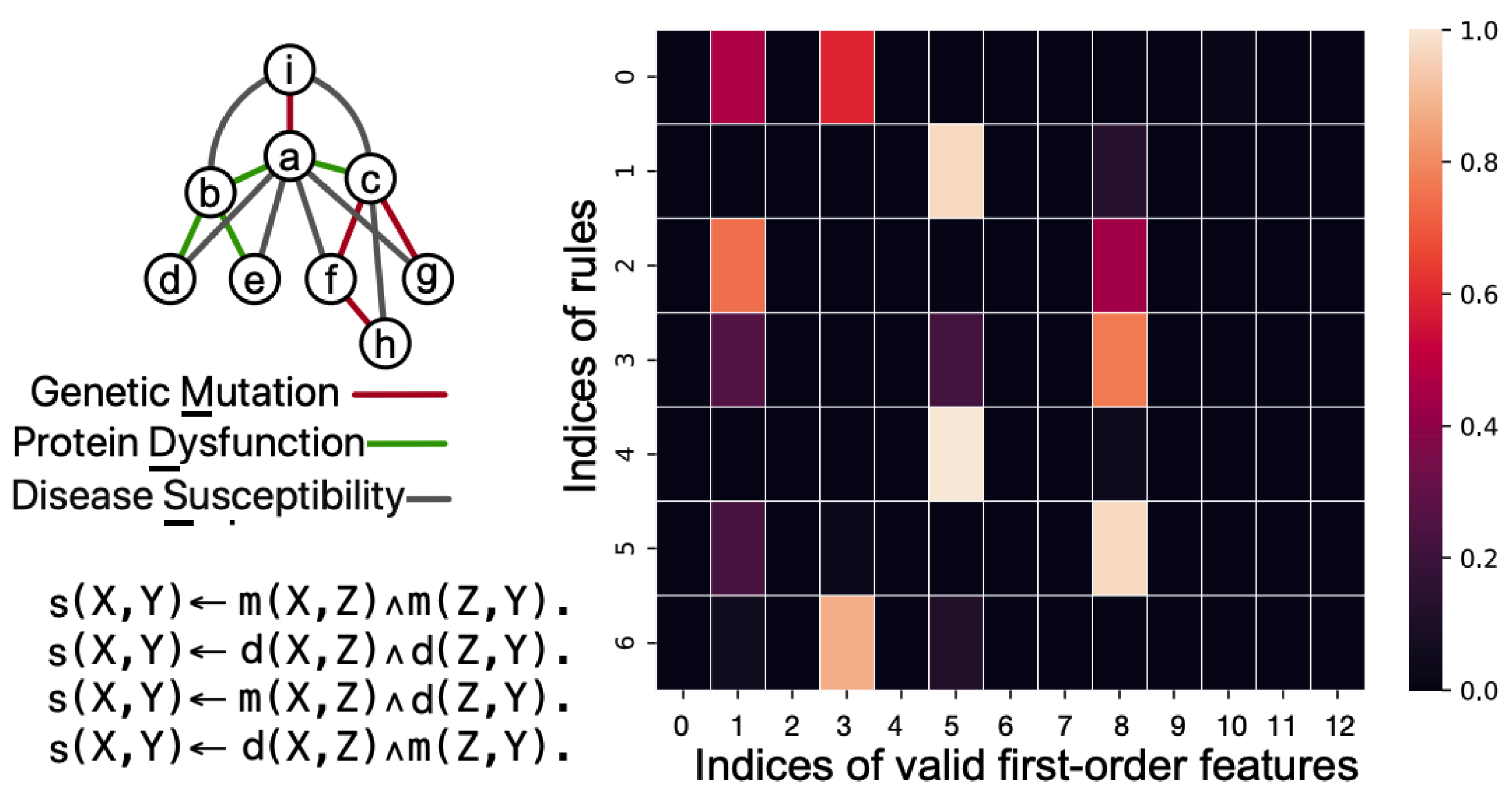
We use the example with the concept of „disease susceptibility.” Specifically, the relation between genetic mutations, the resulting protein dysfunctions, and the diseases they cause can be transitive.
Extracting LPs from a Matrix Obtained by KAN
In this section, we describe how to extract LPs from a trained matrix, following (Gao et al 2022).
In the matrix MP obtained by KAN, the element at the m-th row and n-th column represents the possibility of n-th valid body feature in the m-th rule rm in P. We use multiple thresholds called Now rule filters comprise multiple threshold application, denoted as τf, acting on KAN result MP to extract rules. Rule filters can be in a range 0 … 1 with step 0.1, and let T be the set with all rule filters. For a τf, the valid features in the k-th row of MPare determined as values greater than τf as the elements in the body(rk). Each τf is applied step by step to the trained matrix MP, and a rule set R˜ with m×|T| rules is obtained.
To assess the precision of a rule, nr will be the number of the substitutions that satisfy both the body and the head atom of a rule, and nb will be the number of the substitutions that satisfy only the body of a rule, where the substitutions are computed based on the a priory facts. The ratio is interpreted as the precision of the rule r. A rule is correct with the precision value 1, and a rule is incorrect with the precision value 0. With the precision value in between (0,1), the rule may still be correct due to the incompleteness of the seen facts.
Another threshold named soundness filter τs is needed: rules with precision values no lower than τs are named sound rules and are added to P. To use the curriculum learning strategy, (Gao et al 2022) position the trained rows in MP corresponding to the sound rules into Mprior after every few epochs. The matrix Mprior is considered as the prior knowledge to boost the training process in the consecutive training epochs. When all training epochs are finished, the sound LP is stored in P.
KAN for LP Learning Example
We start with an example of transitive relation in health which can be learned from instances in the form of LP:
- (1)
- Genetic Mutation: A mutation in the BRCA1 gene.
- (2)
- Protein Dysfunction: The mutation in the BRCA1 gene leads to the dysfunction of the BRCA1 protein.
- (3)
- Disease Susceptibility: Dysfunction of the BRCA1 protein increases the susceptibility to breast and ovarian cancer.
The training facts are located at top-left of Figure 14, the learned matrix (at right), and the extracted LP P (at bottom-left) in the grandparent task. The valid first-order features with indices 0-12 are m(X, Y ), m(X, Z), m(Y,Z), m(Z, Y), d(X, Y), d(X, Z), d(Y, Z), d(Z, X), d(Z, Y), s(X, Z), s(Y, Z), s(Z, X), s(Z, Y)
An example of KAN input is as follows:
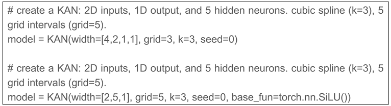
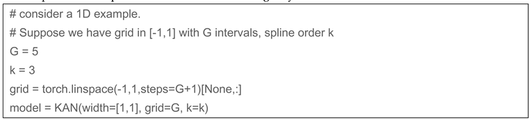
One important feature of KANs is that they embed splines to neural networks. However, splines are only valid for approximating functions in known bounded regions, while the range of activations in neural networks may be changing over training. So we have to update grids properly according to that. Splines can be parameterized in the following way.
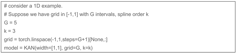
There are G+k B-spline basis. The function is a linear combination of these bases
The activation function has two additive parts, a residual function b(x) plus the spline function, i.e.,
and by default b(x)=silu(x)=x/(1+e−x).
5. Conclusions
The connection between the Kolmogorov-Arnold theorem and neural networks is not new, but the peculiar features of inner functions make this theorem impractical for application (Poggio 2022). Previous research primarily employed the original 2-layer width-(2n + 1) networks, which are limited in expressive power and many predate backpropagation. Liu et al. (2024) generalized the network architecture to higher dimensions, situating KANs within the modern deep learning context and highlighting their potential role as a foundation model for AI, emphasizing interactivity with human developers and explainability.
Both MLPs and KAN models theoretically can represent any function. However, in practice, large MLPs tend to exhibit high variance, requiring substantial data to correct errors. Despite attempts at regularization, mitigating this issue effectively remains challenging. In contrast, KAN models offer a novel approach to learning complex mappings from inputs to outputs with significantly fewer parameters. These networks require less regularization and data to efficiently discern statistical patterns. Traditional MLPs frequently use Rectified Linear Unit (ReLU) activation functions for their computational efficiency, though this choice can lead to sluggish training of affine functions.
KAN can serve as the foundation of a Transformer with a Mixture-of-Experts architecture, where the experts are feedforward networks composed of KAN layers. A Rotary Position Embedding can encode token positions, and the attention mechanism is a vanilla multihead-attention layer with a KAN layer as the query-key-value projector. Linear layers with KAN layers demonstrate how straightforward it is to use this new tool. An efficient implementation of the KAN network is available (Blealtan 2024, Liu 2024).
We developed a hybrid system that combines the interpretability and rule-based reasoning of logic programming with the predictive accuracy and adaptability of neural networks. This integration aims to deliver robust, transparent, and reliable AI solutions across various application domains such as health.
A differentiable first-order rule learner is integrated with KAN, enabling it to learn first-order logic programs in a forward-chained format from relational facts without relying on logic templates. This method translates relational data into a neural network-compatible format, similar to KAN-readable data. Symbolic logic programs can be directly extracted from the trainable matrices, and prior knowledge can be applied as constraints to implement curriculum learning. In curriculum learning, the model is exposed to training data in a specific sequence, starting with simpler examples and progressively moving to more complex ones. This approach mirrors human learning, beginning with basic concepts and gradually tackling more difficult tasks as knowledge and skills build.
References
- Blealtan (2024) An Efficient Implementation of Kolmogorov-Arnold Network https://github.com/Blealtan/efficient-kan/tree/master.
- Bohra, P.; Campos, J.; Gupta, H.; Aziznejad, S.; Unser, M. Learning Activation Functions in Deep (Spline) Neural Networks. IEEE Open J. Signal Process. 2020, 1, 295–309. [Google Scholar] [CrossRef]
- Garcez, A.D.; Broda, K.; Gabbay, D. Symbolic knowledge extraction from trained neural networks: A sound approach. Artif. Intell. 2001, 125, 155–207. [Google Scholar] [CrossRef]
- Evans, R.; Grefenstette, E. Learning Explanatory Rules from Noisy Data. J. Artif. Intell. Res. 2018, 61, 1–64. [Google Scholar] [CrossRef]
- Fakhoury, D.; Fakhoury, E.; Speleers, H. ExSpliNet: An interpretable and expressive spline-based neural network. Neural Networks 2022, 152, 332–346. [Google Scholar] [CrossRef] [PubMed]
- Fifth ACM SIGKDD International Conference on Knowledge Discovery and Data Mining, pages 194{200. ACM, 1999.
- Gao, K.; Wang, H.; Cao, Y.; Inoue, K. Learning from interpretation transition using differentiable logic programming semantics. Mach. Learn. 2021, 111, 123–145. [Google Scholar] [CrossRef]
- Gao, K & Inoue, Katsumi & Cao, Yongzhi & Wang, Hanpin. (2022). Learning First-Order Rules with Differentiable Logic Program Semantics. 2983-2989. [CrossRef]
- Hastie T., J. and R. J. Tibshirani. Generalized Additive Models. Chapman and Hall, 1990.
- Igelnik, B. and N. Parikh. Kolmogorov’s spline network. IEEE Transactions on Neural Networks, 14:725–733, 2003.
- International Conference on Computer Vision, pages 1467-1475. IEEE, 2015.
- Kaminski, T.; Eiter, T.; Inoue, K. Exploiting Answer Set Programming with External Sources for Meta-Interpretive Learning. Theory Pr. Log. Program. 2018, 18, 571–588. [Google Scholar] [CrossRef]
- Kontschieder P, M. Fiterau, A. Criminisi, and S. R. Bul`o. Deep neural decision forests. In Proceedings of the IEEE International Conference on Computer Vision, 2015., pages 1467– 1475. IEEE. [Google Scholar]
- Kontschieder P, M. Fiterau, A. Criminisi, and S. R. Bulo. Deep neural decision forests. In Proceedings of the IEEE.
- Kramer S, Nada Lavrac, and Peter Flach. Propositionalization approaches to relational data mining, pages 262–291. Springer, Berlin: Heidelberg, 2001.
- Lehmann, J.; Bader, S.; Hitzler, P. Extracting reduced logic programs from artificial neural networks. Appl. Intell. 2008, 32, 249–266. [Google Scholar] [CrossRef]
- Liu Z (2024) Kolmogorov Arnold Networks https://github.
- Lyche T, C. Manni, and H. Speleers. Foundations of spline theory: B-splines, spline approximation, and hierarchical refinement. In T. Lyche, C. Manni, and H. Speleers, editors, Splines and PDEs: From Approximation Theory to Numerical Linear Algebra, volume 2219 of Lecture Notes in Mathematics, pages 1–76. Springer International Publishing, 2018.
- Lyche T, C. Manni, and H. Speleers. Foundations of spline theory: B-splines, spline approximation, and hierarchical refinement. In T. Lyche, C. Manni, and H. Speleers, editors, Splines and PDEs: From Approximation Theory to Numerical Linear Algebra, volume 2219 of Lecture Notes in Mathematics, pages 1{76. Springer International Publishing, 2018.
- Poggio T, Andrzej Banburski, and Qianli Liao. Theoretical issues in deep networks. Proceedings of the National Academy of Sciences, 117(48):30039–30045, 2020.
- Poggio, T. How deep sparse networks avoid the curse of dimensionality: Efficiently computable functions are compositionally sparse. CBMM Memo, 10:2022, 2022.
- Potts W. J., E. (1999) Generalized additive neural networks. In S. Chaudhuri and D.
- Potts W. J., E. Generalized additive neural networks. In S. Chaudhuri and D. Madigan, editors, Proceedings of the Fifth ACM SIGKDD International Conference on Knowledge Discovery and Data Mining, pages 194–200.; p. 1999.
- Ribeiro M, S. Singh, and C. Guestrin. “Why should I trust you”: Explaining the predictions of any classifier. In J. DeNero, M. Finlayson, and S. Reddy, editors, Proceedings of the 2016 Conference of the North American Chapter of the Association for Computational Linguistics: Demonstrations, pages 97–101.; p. 2016.
- Rudin, C. Stop explaining black box machine learning models for high stakes decisions and use interpretable models instead. Nat. Mach. Intell. 2019, 1, 206–215. [Google Scholar] [CrossRef] [PubMed]
- Sakama, C.; Inoue, K.; Sato, T. Logic programming in tensor spaces. Ann. Math. Artif. Intell. 2021, 89, 1133–1153. [Google Scholar] [CrossRef]
- Sande, E.; Manni, C.; Speleers, H. Sharp error estimates for spline approximation: Explicit constants, n-widths, and eigenfunction convergence. Math. Model. Methods Appl. Sci. 2019, 29, 1175–1205. [Google Scholar] [CrossRef]
- Shindo H, Masaaki Nishino, Akihiro Yamamoto (2021) Differentiable Inductive Logic Programming for Structured Examples. arXiv:2103. 0171.
- Shindo, H.; Nishino, M.; and Yamamoto, A. 2018. Using Binary Decision Diagrams to Enumerate Inductive Logic Programming Solutions. In 28th International Conference on Inductive Logic Programming (ILP 2018), 52–67.
- Van Emden, M.H.; Kowalski, R.A. The Semantics of Predicate Logic as a Programming Language. J. ACM 1976, 23, 733–742. [Google Scholar] [CrossRef]
- Wan, L. , Zeiler, M.D., Zhang, S., LeCun, Y., & Fergus, R. (2013). Regularization of Neural Networks using DropConnect. International Conference on Machine Learning.
Figure 2.
Activation structure of the network.
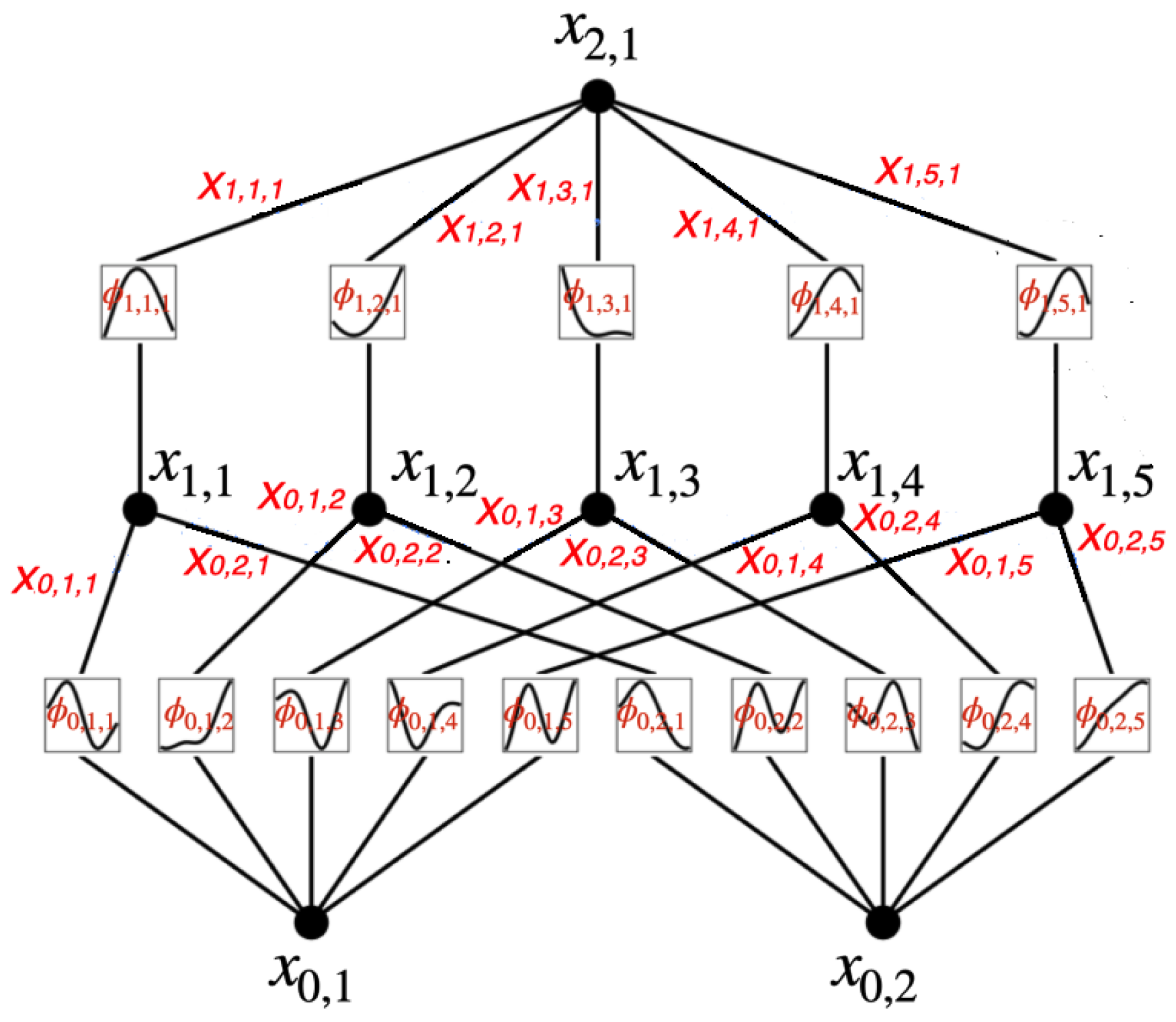
Figure 3.
An activation function is parameterized as a B-spline, which allows switching between coarse-grained and fine-grained grids.
Figure 3.
An activation function is parameterized as a B-spline, which allows switching between coarse-grained and fine-grained grids.
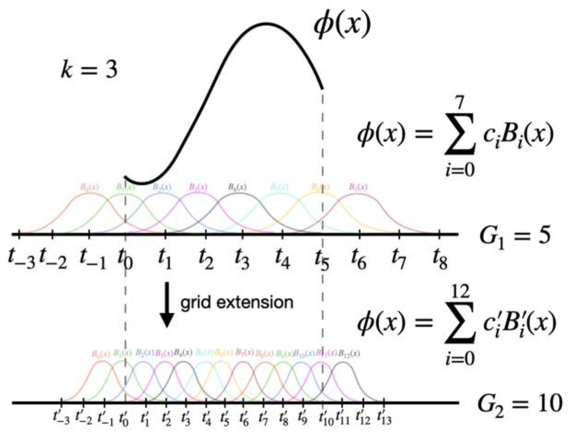
Figure 4.
B-splines in the vectors for N = 10, p = 1, 2, 3, and x ∈ [0, 1].
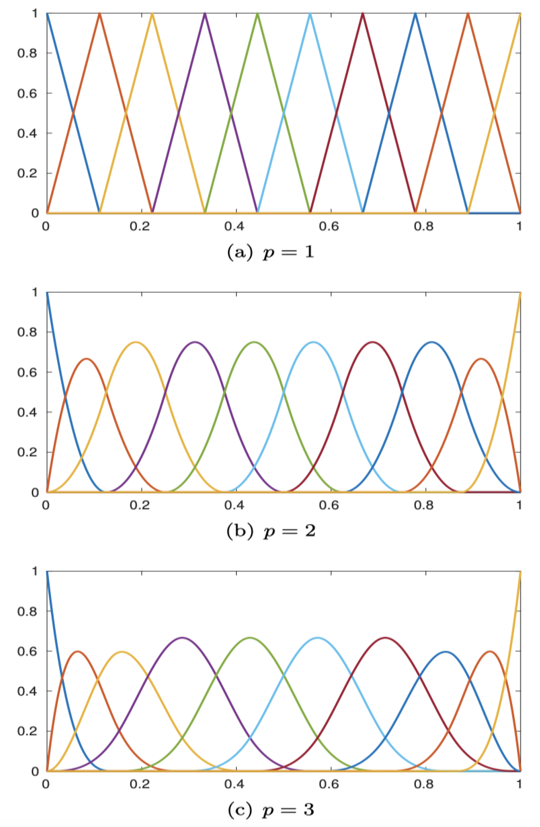
Figure 5.
A tree structure consisting of L = 2 levels.
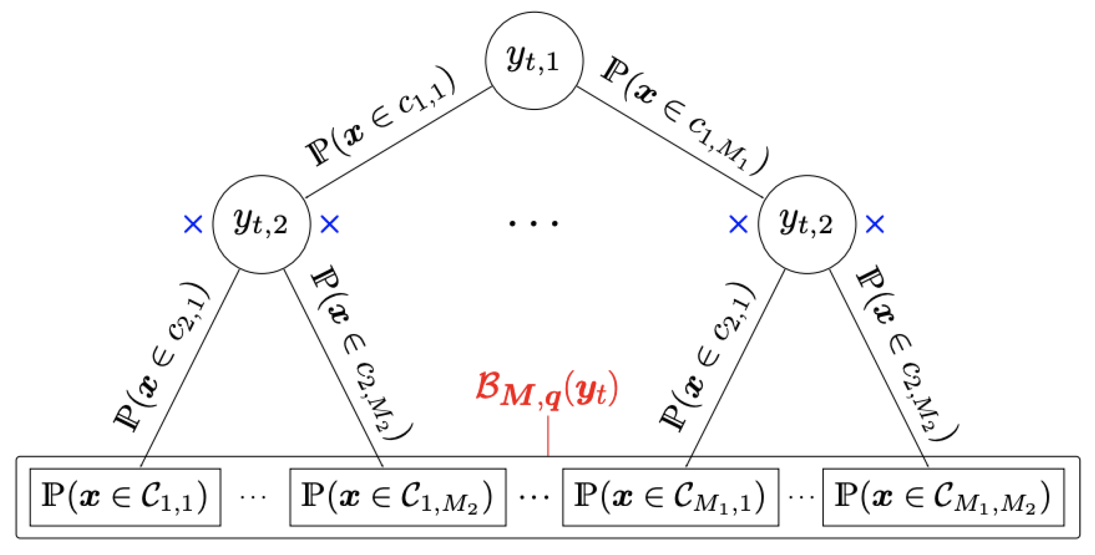
Figure 7.
A symbolic regression of a continuous function.
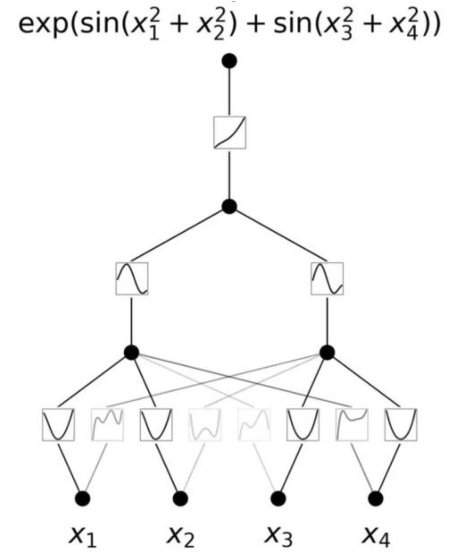
Figure 8.
symbolic regression with KAN and supporting user interactions.
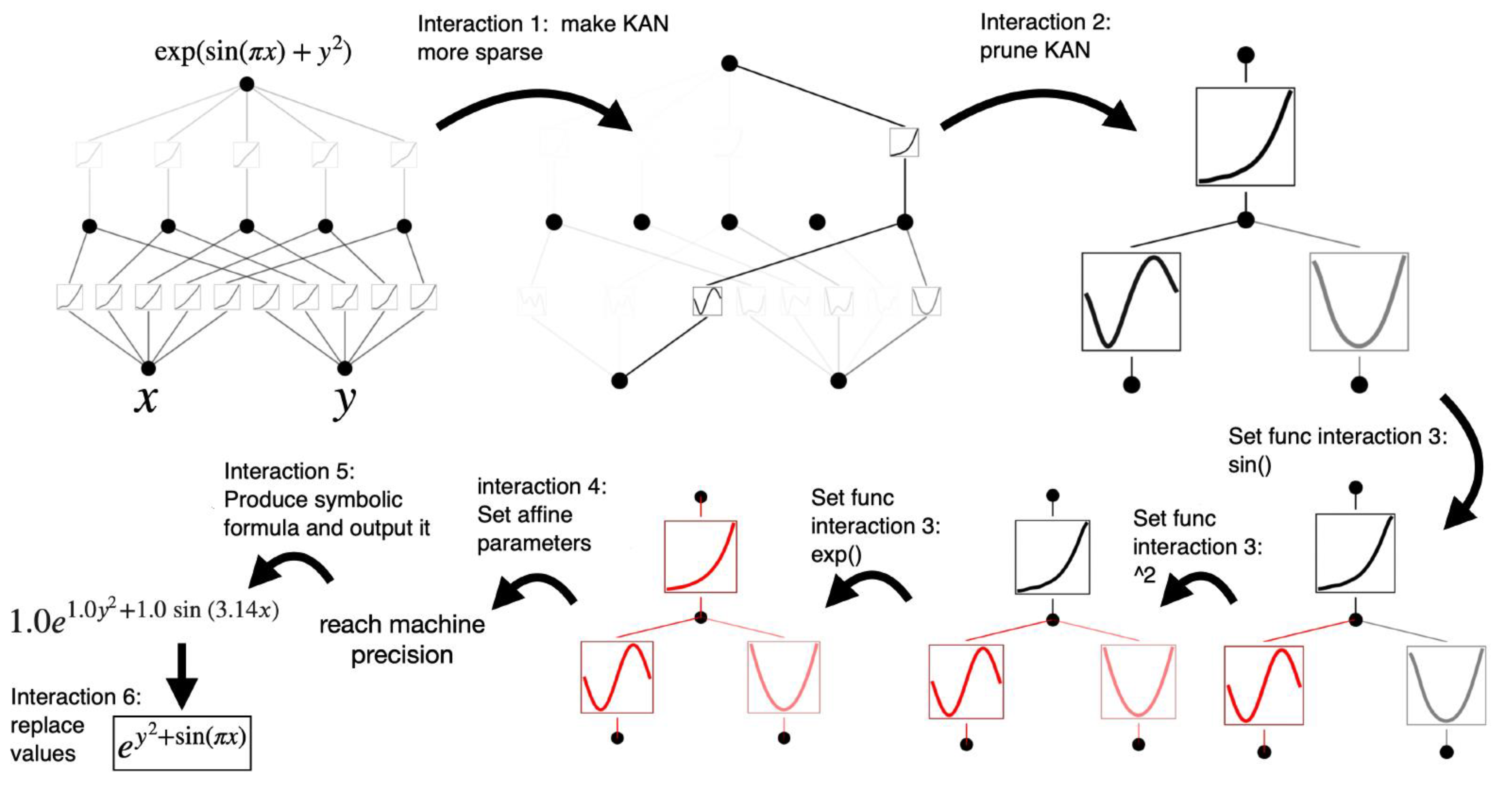
Figure 9.
Word2vec continuous profiles of words.
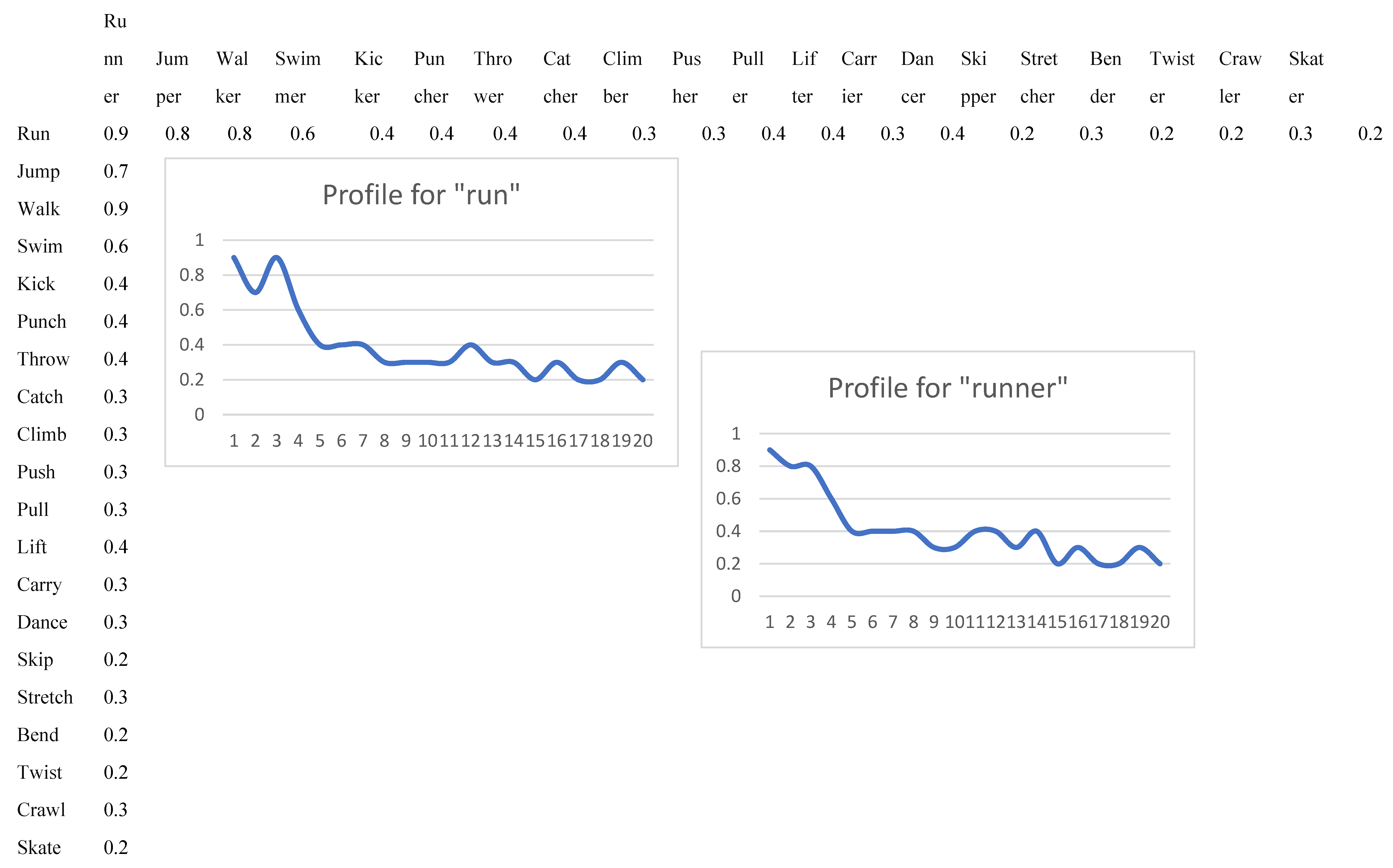
Figure 10.
KAN network for word-based symbolic regression.
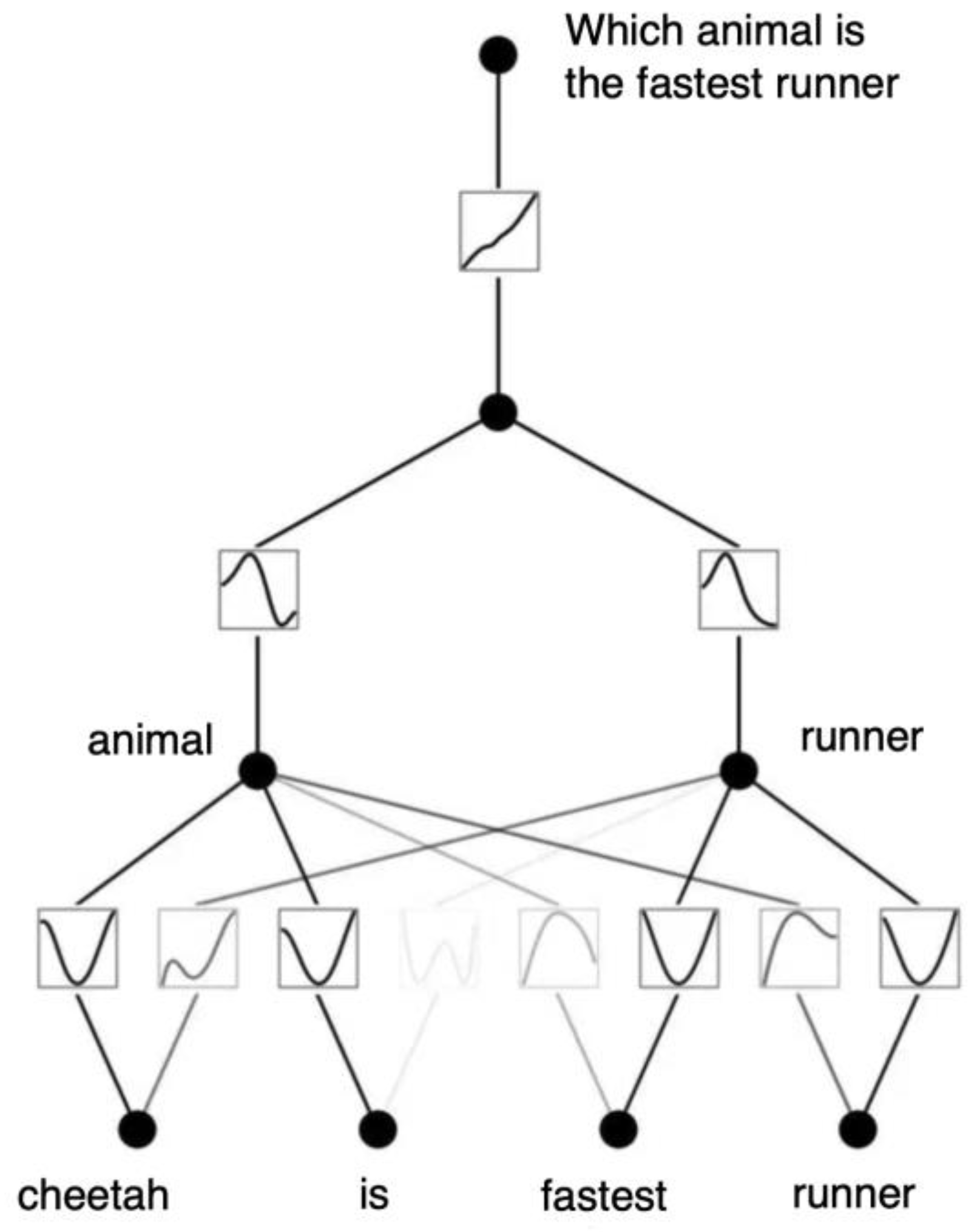
Figure 11.
KAN network solving a masking problem.
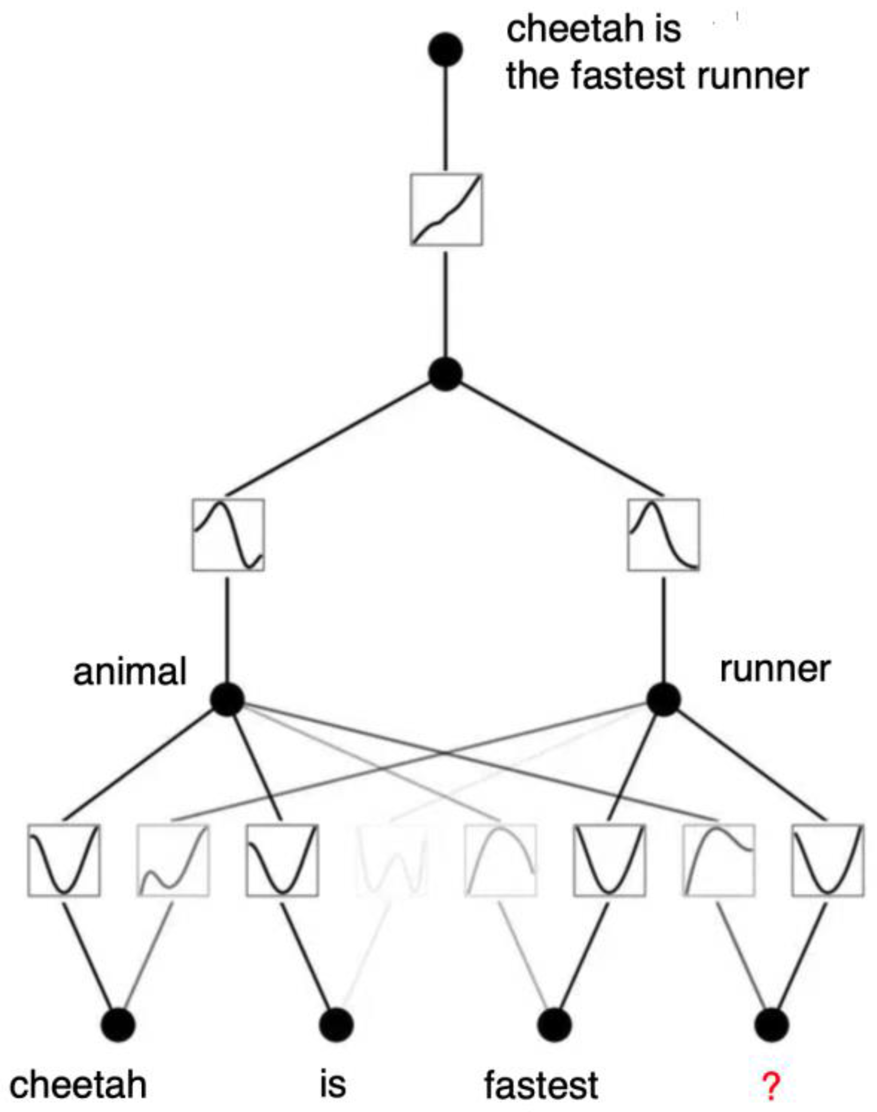
Figure 13.
Architecture of ∂ILP.
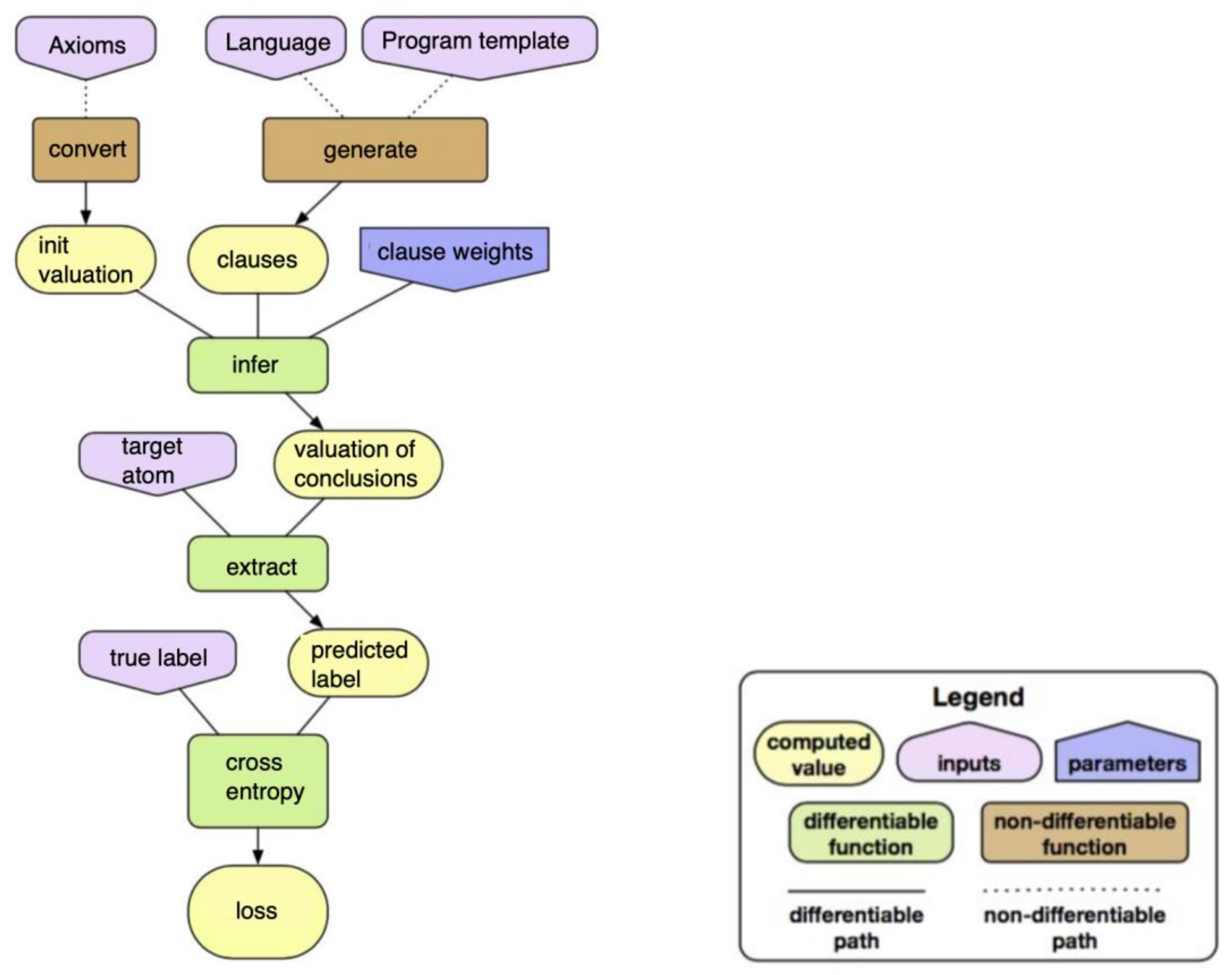
Figure 14.
Beam searching for clauses.
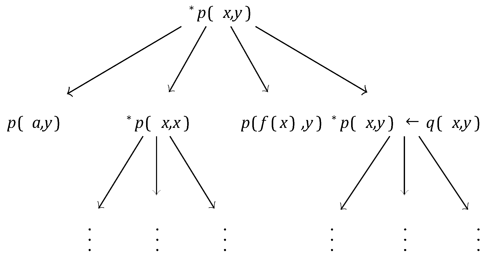
Figure 14.
Encoding of LP as a matrix of indices.
Disclaimer/Publisher’s Note: The statements, opinions and data contained in all publications are solely those of the individual author(s) and contributor(s) and not of MDPI and/or the editor(s). MDPI and/or the editor(s) disclaim responsibility for any injury to people or property resulting from any ideas, methods, instructions or products referred to in the content. |
© 2024 by the authors. Licensee MDPI, Basel, Switzerland. This article is an open access article distributed under the terms and conditions of the Creative Commons Attribution (CC BY) license (http://creativecommons.org/licenses/by/4.0/).
Copyright: This open access article is published under a Creative Commons CC BY 4.0 license, which permit the free download, distribution, and reuse, provided that the author and preprint are cited in any reuse.


