
Submitted:
31 January 2026
Posted:
03 February 2026
You are already at the latest version
Abstract
This work addresses the design of a predefined-time adaptive fuzzy control scheme for
high-order nonlinear systems with nonstrict-feedback structures, subject to unmodeled dynamics and input time delay. To mitigate the influence of unmodeled dynamics, a predefined-time auxiliary dynamic signal is incorporated into the controller design. Meanwhile, the adverse effects caused by input delay are handled by integrating a Padé approximation with the introduction of an intermediate state variable. Fuzzy logic systems are utilized to approximate the unknown nonlinear terms present in the system dynamics. Based on a recursive backstepping framework and a power-type Lyapunov function formulation, an adaptive fuzzy tracking controller with predefined-time convergence char acteristics is constructed. A detailed stability analysis demonstrates that the closed-loop system achieves practical predefined-time convergence, and appropriate selection of design parameters guarantees that the tracking errors remain confined within a small bounded region around the origin. Finally, the effectiveness and advantages of the proposed control strategy are validated through a numerical example and a practical example.
Keywords:
nonlinear systems
; adaptive control
; predefined-time stability
; unmodeled dynamics
; input delay
MSC: 93C10; 93C40; 37N35
1. Introduction
The control of high-order nonlinear systems has attracted sustained attention due to their broad applicability in complex engineering processes. Compared with strict-feedback systems, high-order nonlinear systems exhibit a more general structure, allowing them to describe intricate nonlinear dynamics more accurately. However, conventional linearization techniques often lead to uncontrollable or unobservable modes, which significantly complicates controller design [1,2,3]. To address these challenges, a constructive control framework based on the adding one power integrator technique was developed, enabling effective stabilization and tracking of high-order nonlinear systems. This approach has been widely extended to adaptive control designs for uncertain systems. Nevertheless, many existing methods rely on precise knowledge of system nonlinearities, an assumption that is difficult to satisfy in practical applications due to modeling uncertainties and external disturbances. To overcome this limitation, intelligent adaptive control schemes employing fuzzy logic systems and neural networks have been introduced. Owing to their strong learning and approximation capabilities, these methods can estimate unknown nonlinear functions online, thereby improving robustness and tracking performance for high-order nonlinear systems with unknown dynamics. Several studies have explored specific adaptive control strategies to handle these challenges in different contexts [4,5]. For example, an adaptive control strategy for high-order nonlinear multi-agent systems operating under event-triggered communication protocols has been reported to decrease communication load while maintaining coordinated tracking accuracy [6]. To overcome the well-known complexity growth associated with backstepping methods, an adaptive dynamic surface control approach incorporating parameter estimation has been proposed for high-order strict-feedback nonlinear systems [7]. Furthermore, an adaptive neural control framework with dynamic memory and event-triggered mechanisms has been introduced for high-order stochastic nonlinear systems subject to delayed output constraints, effectively addressing stochastic disturbances and constraint requirements in a unified manner [8]. Additionally, adaptive tracking control schemes for high-order nonlinear systems with time-varying delays and asymmetric output constraints have been investigated, ensuring robust tracking performance in the presence of delay effects and nonuniform constraint limits [9].
Due to modeling inaccuracies, external disturbances, measurement noise, and inevitable modeling simplifications, unmodeled dynamics frequently exist in practical control systems. These neglected dynamics, such as unknown high-order system behaviors, actuator dynamics, and unaccounted nonlinear effects, introduce additional uncertainties that are not represented in the nominal model [10,11,12]. As a consequence, the presence of unmodeled dynamics can degrade tracking accuracy, slow system responses, and in severe cases, lead to instability of the controlled plants [13,14]. Therefore, considerable research attention has been devoted to the study of nonlinear systems with unmodeled dynamics, with the objective of developing robust and adaptive control strategies that can effectively compensate for these uncertainties while guaranteeing stability and satisfactory control performance. Several studies have explored specific adaptive control strategies to address unmodeled dynamics in various contexts [15,16,17]. As an example, adaptive control scheme has been reported for nonlinear systems with input time delays, unknown dead-zone characteristics, and unmodeled dynamics, aiming to simultaneously counteract delay effects, actuator nonlinearities, and modeling inaccuracies [18]. To enhance approximation accuracy and fault-handling capability in fractional-order systems, neural network–based adaptive controller has been introduced for nonlinear dynamics affected by actuator faults and unmodeled uncertainties [19]. Moreover, event-triggered fuzzy adaptive finite-time control strategy has been proposed for stochastic nonlinear systems with unmodeled dynamics, enabling rapid convergence while alleviating communication and computational overhead [20]. Furthermore, adaptive control approach for pure-feedback nonlinear systems under full-state time-varying constraints and unmodeled dynamics has been developed to ensure closed-loop stability and continuous satisfaction of state constraints despite structural uncertainties and evolving limitations [21].
Input delay is an inevitable factor that adversely affects the control accuracy of practical systems due to limitations in actuators, communication channels, and hardware implementation [22]. The existence of input delay can significantly degrade transient response and tracking performance, and may even result in instability if not properly addressed. To mitigate the adverse effects of input delay, various compensation and approximation-based control strategies have been proposed [23,24]. Among them, the Padé approximation method has been widely adopted to transform the delayed input into an equivalent delay-free form, which greatly simplifies controller design. By incorporating Padé approximation into adaptive control frameworks, the influence of input delay in nonlinear systems can be effectively reduced, leading to improved control performance and enhanced closed-loop stability. Several studies have explored specific adaptive control strategies to address input delays in various contexts [25,26,27]. For instance, a finite-time adaptive prescribed performance control has been developed for nonlinear systems with input delay to ensure rapid convergence while compensating for delayed control actions [28]. Adaptive tracking control for nonlinear systems affected by input delay and dynamic uncertainties has been investigated by employing multi-dimensional Taylor network approximations to enhance modeling accuracy and robustness [29]. Neural network–based adaptive reinforcement learning approaches have been explored to achieve optimized backstepping tracking control for nonlinear systems with input delay, enabling online performance improvement through learning mechanisms [30]. In addition, adaptive neural control has been studied for non-strict feedback stochastic nonlinear systems with input delay to handle randomness and delayed inputs while guaranteeing stability and satisfactory tracking behavior [31].
Finite-time control has attracted considerable attention because it guarantees system convergence within a finite duration, providing faster response than asymptotic stabilization methods. It is well known that the convergence time associated with finite-time control schemes is typically a function of the system’s initial conditions, which limits their effectiveness in applications requiring a uniform convergence duration. To address this limitation, fixed-time control was proposed, where the convergence time is explicitly decoupled from the initial state of the system [32,33]. By suitably selecting the control laws, fixed-time strategies guarantee that all system trajectories reach the desired equilibrium within a prescribed bounded time interval. Nevertheless, the convergence time in fixed-time control still depends on several design parameters, and the theoretically derived upper bound is often overly conservative, resulting in a mismatch between analytical estimates and the observed convergence behavior in practical implementations [34,35,36]. In many practical applications, such as aircraft attitude control, multi-agent coordination, and cooperative robotic systems, stability must be achieved within a prescribed time interval. Neither finite-time control nor fixed-time control can guarantee convergence within an exact predefined duration. To eliminate the dependence of convergence time on initial conditions, predefined-time control was introduced, wherein the settling time is exclusively determined by a tunable control parameter rather than the system’s initial state [37,38,39]. This property enables the convergence duration to be explicitly specified a priori, rendering predefined-time control highly attractive for applications with stringent time-performance constraints. In recent years, a variety of adaptive predefined-time control frameworks have been reported for different classes of nonlinear systems [40,41,42,43]. As representative examples, predefined-time adaptive fuzzy control scheme has been developed for nonlinear systems subject to input saturation and delayed constraints, guaranteeing convergence within a designer-assigned time interval even in the presence of actuator limitations [44]. Moreover, adaptive predefined-time control approach has been proposed for stochastic switched nonlinear systems with full-state error constraints and input quantization, ensuring prescribed convergence behavior under switching dynamics and quantization effects [45]. Additionally, adaptive fuzzy predefined-time control strategy has been investigated for stochastic nonlinear systems experiencing actuator and sensor faults, thereby achieving fault-tolerant operation while preserving predefined-time stability [46]. Furthermore, adaptive fuzzy predefined-time tracking controller has been designed for nonstrict-feedback high-order nonlinear systems with input quantization, attaining accurate tracking performance within a predefined time bound despite system complexity and quantization-induced nonlinearities [47].
The motivation for this work stems from the persistent challenges encountered in controlling high-order nonlinear systems under realistic operating conditions. Despite significant advancements in adaptive control, many practical systems continue to suffer from uncertainties arising from unmodeled dynamics, input delays, actuator nonlinearities, and structural complexities. Existing control strategies, including finite-time and fixed-time approaches, often fail to guarantee precise convergence within a user-specified duration, limiting their applicability in safety-critical and time-sensitive applications such as aerospace systems, multi-agent coordination, and cooperative robotics. Moreover, while intelligent adaptive techniques using fuzzy logic systems and neural networks have improved robustness and approximation capabilities, integrating these methods with rigorous time-performance guarantees remains an open problem. These gaps inspired the present research to develop a predefined-time adaptive fuzzy control framework that simultaneously addresses high-order nonlinear dynamics, input delays, and unmodeled uncertainties, with the objective of achieving accurate, reliable, and fast tracking within a rigorously prescribed time interval. This work is further motivated by the need for a control approach that combines the flexibility of intelligent approximation with the predictability of predefined-time convergence, offering practical utility in complex, uncertain, and delayed nonlinear systems. Based on the above analysis, this study is devoted to the design of a predefined-time control framework for high-order nonlinear systems affected by dynamic uncertainties and input time delays. In contrast to the existing literature, the key contributions of this work can be outlined as follows
- (i)
- Relative to the control schemes presented in [31,32], this work investigates a predefined-time adaptive fuzzy control problem for high-order nonstrict-feedback nonlinear systems in the presence of unmodeled dynamics and input time delays. In contrast to finite-time and fixed-time control approaches reported in [33,34,35,36], the proposed method guarantees system stabilization within a designer-assigned time horizon. Specifically, the convergence duration is directly governed by a tunable design parameter, enabling its explicit selection prior to controller implementation to satisfy desired performance specifications. To enhance practical feasibility, a Padé approximation technique is employed to address the adverse effects of input delays. This delay-compensation mechanism ensures that the closed-loop system retains stability and satisfactory tracking performance even when control actions are subject to delays. Consequently, the developed control framework is applicable to a wide range of high-order nonlinear systems where input delay effects are unavoidable.
- (ii)
- A dynamic control signal based on the predefined-time control principle is designed to address the effects of unmodeled dynamics, including unknown high-order system behaviors and actuator nonlinearities. The control law ensures that the closed-loop system achieves practical predefined-time stability, meaning that system states converge to a small neighborhood around the origin within the specified time. By selecting appropriate control parameters, the tracking performance can be effectively improved, and the impact of modeling uncertainties, external disturbances, and unmodeled dynamics can be minimized. This provides both theoretical assurance and practical feasibility for high-precision control of complex nonlinear systems.
The remainder of this paper is organized as follows. Section 2 presents the problem formulation along with the required preliminary concepts. The design of the adaptive tracking controller and the associated stability analysis are detailed in Section 3. Simulation results and a representative practical application are provided in Section 4 to demonstrate the performance of the proposed method. Finally, Section 5 concludes the paper and outlines potential directions for future investigation.
2. Problem Formulation and Preliminaries
Consider a class of high-order nonlinear systems with a nonstrict-feedback structure, which can be expressed as
where the system state vector is defined as , with the partial state vector . The constants are odd integers. The functions denote unknown smooth nonlinearities satisfying . The variable represents unmeasured internal state dynamics, where the -subsystem corresponds to unmodeled dynamics. The terms describe unknown nonlinear disturbances acting on the system. It is assumed that and are uncertain but locally Lipschitz continuous. The scalar variables and denote the control input and system output, respectively. represents an unknown input delay, which is assumed to be a positive constant.
To address the input delay appearing in the high-order nonlinear system (1), the Padé approximation technique is employed, following the approach in [22]. By virtue of the delay property of the Laplace transform, the following relationship holds:
where denotes the Laplace variable. Using the first-order Padé approximation, one has
where is the Laplace transform of .
Remark 1.
Due to the inherent limitation of the Padé approximation, the proposed approach is applicable to systems with small input delays. When is sufficiently small, the approximation error is negligible. The extension to large or time-varying delays will be investigated in future work.
To facilitate controller design, an auxiliary state is introduced such that
Rearranging the above equation yields
Applying the inverse Laplace transform gives
Define , then the above equation can be rewritten as
Following the aforementioned transformations, the delayed system in (1) can be reformulated into an equivalent delay-free augmented representation given by
The objective of this study is to develop a predefined-time adaptive control strategy based on fuzzy logic systems for system (1), such that all closed-loop signals remain bounded within a designer-specified time interval, and the output tracking error converges to a sufficiently small neighborhood of the origin.
Assumption 1
[13]: For each , ∃ known, smooth, and nonnegative functions and satisfying
Moreover, without imposing any restriction on generality, the function is assumed to satisfy .
Assumption 2
[14]: Consider the -subsystem associated with system (1). There exist class functions , , and , together with positive constants a and , such that an exponentially input-to-state practically stable (Exp-ISpS) Lyapunov function can be constructed satisfying
and
Assumption 3
[48]: Define , for , as positive odd integers, and let . The odd integers satisfy the inequality
Assumption 4
[36]: The reference trajectory , together with its derivative of order h, is assumed to be smooth and uniformly bounded for all time.
Lemma 1
[49]: Given arbitrary real scalars and , and any prescribed positive constants , , and , the following result holds
Lemma 2
[39]: Assume that conditions (10) and (11) are satisfied. Under these conditions, the function qualifies as an exponentially input-to-state practically stable (Exp-ISpS) Lyapunov function for the subsystem . Let and be positive constants satisfying , and define . For any initial time and initial condition , and for any continuous function satisfying , there exists a predefined time , a positive constant , and a nonnegative function defined for all , such that the auxiliary signal satisfies
Moreover, the function satisfies , and the Lyapunov function is bounded by
The solution of the system exists for all . Without loss of generality, the function is chosen as under which the auxiliary dynamic signal can be rewritten as
where denotes a smooth nonnegative function.
Lemma 3
[39]: For arbitrary real-valued functions and , any odd integer , and a given constant , one has
where for , and for . In this work, the exponent is selected as . For notational convenience, both cases are unified as
Lemma 4
[50]: Let and be constants, and define the set , . Then, for all , the inequality is satisfied.
Lemma 5
[39]: For any and any constant , the following inequality holds .
Lemma 6
[39]: Let be an unknown continuous function defined on a compact set . For any prescribed constant , there exists a fuzzy logic system (FLS) of the form such that
where denotes the adjustable weight vector, and represents the minimum approximation error. Moreover, is the number of fuzzy inference rules. The fuzzy basis function vector is defined as , where each basis function is selected as a Gaussian membership function given by
with and denoting the center and width parameters of the Gaussian function, respectively.
Lemma 7
[39]: Let be the input vector, and let denote the corresponding fuzzy basis function vector. For any positive integer , define . Then, the following inequality holds:
Consider the nonlinear dynamical system
where denotes the state vector, the origin is an equilibrium point, and is a nonlinear mapping.
Definition 1
[39]: Let and be given constants. If the state trajectory o satisfies for all , then the equilibrium point at the origin is said to be practically predefined-time stable. The constant is referred to as the predefined time.
Lemma 8
[39]: Assume that there exists a Lyapunov function such that
where , and and B are strictly positive constants. Under these conditions, the function V guarantees practical predefined-time stability, and the corresponding settling time is bounded above by .
3. Controller Design and Stability Analysis
To facilitate the construction of the desired control law, the following error coordinate transformations are introduced
where denotes the virtual control signal to be designed subsequently.
Step 1: From (1) and (25), the time derivative of is obtained as
To analyze the stability of the first subsystem, consider the following power-type Lyapunov function
where is the estimate of the unknown parameter and denotes the corresponding estimation error. The design parameters and are chosen as positive constants. By invoking Assumption 1 together with (16), the time derivative of the Lyapunov function satisfies
Applying Lemma 5, the term can be upper bounded as
where is a design constant, , and .
By utilizing Assumption 2 together with Lemmas 2 and 5, and following estimation techniques similar to those developed in [26], the following upper bound can be derived:
where is a design parameter, and denotes the inverse of the function introduced in Assumption 2. The estimated function is defined as , with . Moreover, the composite function , and , where for all .
Remark 2:
It is worth noting that the term is discontinuous at , which prevents its direct approximation using fuzzy logic systems. To overcome this difficulty, a smooth hyperbolic tangent function with a given constant is introduced. As a result, the expression becomes well defined and continuous at .
By using (29) and (30) into (28), one has
where .
Based on Lemma 6, the unknown smooth nonlinear function is approximated using a fuzzy logic system (FLS) expressed in the form
where is the FLS input vector, denotes the ideal weight vector, and represents the fuzzy approximation error satisfying , with being a known constant.
By applying Young’s inequality together with Lemma 7, the following bounds can be established:
where , is a design constant, and denotes an unknown bound satisfying .
By using (26) into (24), one has
Furthermore, by applying Young’s inequality, for any , one has
The virtual control law and the adaptive update law for the parameter estimate are designed as
where , , , , , and the initial condition satisfies .
By using (35)-(37) into (34), one has
Using Lemmas 1 and 3, one has
where is a positive constant related to the given constants and and is a nonnegative function.
By using (39) into (38), we have
Applying Lemma 1, one has
Next, the time derivative of can be calculated as
Setting , one obtains
where and are positive constants.
For (43), let us set . Defining and , we obtain
Similarly, for , if we choose and , we have
By using (43)–(45) into (42), one has
where .
Step (): By using (1) and (18), the derivative of is
where
Consider the following Lyapunov function as
where is the estimate of , , and is a designed parameter.
Let be defined as . By invoking Assumption 2 together with Lemmas 2 and 5, and by applying arguments similar to those presented in Step 1, one has
where , , , , , , ,
Using the results given in (47)–(50), the time derivative of can be expressed as
where .
Now, can be estimated through a fuzzy logic system (FLS) approximation of the form
where and is a constant.
With the help of Young’s inequality and Lemma 7, one has
where , , is a design parameter, and satisfies .
The virtual controller and the adaptive law for are designed as
where , , and . Moreover, , , and is a nonnegative constant under Assumption 3. In addition, ,
and .
By using (53)–(55) into (51), one has
By Lemma 1 and Lemma 3, one has
where , which is a positive constant related to the given constants and , and , where is a nonnegative function.
Furthermore, by Lemma 1, we have
where .
By using (57) and (58) into (56), one has
Using (44) and (45) into (59), one has
where .
Step h: By using (8) and (25), one has
where is defined analogously to in Step .
Consider the following Lyapunov function as
where is the estimation of , , and is a designed positive parameter.
Define . Similar to Step 1, one has
where ,, , , , , .
By using (63) and differentiating , one has
where denotes a nonnegative constant and
Now, can be approximated by the FLS as
where and is a constant.
With the help of Young’s inequality and Lemma 7, one has
By using (67) into (65), one has
The real control u and the adaptive law are formulated as
where , , and , and .
By using (69) into (70), one has
From Lemma 1, we have
By using (44), (45), and (72) into (71), one has
where
Consider the complete Lyapunov function as
According to [39], there exists a positive constant such that the parameter estimation error satisfies . Invoking Lemma 1 and choosing , , , and , one has
Based on the inequalities in [39], it follows that
where for all .
By employing (75)–(78) and differentiating V, one obtains
where .
Theorem 1:
For the nonlinear system described in (1), suppose that Assumptions 1–4 hold. When the control inputs are designed according to (36), (54), and (69), and the adaptive update mechanisms are selected as in (37), (55), and (69), it follows that, starting from bounded initial states, every signal of the resulting closed-loop system remains bounded. Moreover, the tracking error is driven into a sufficiently small neighborhood of the origin within a user-prescribed finite time interval.
Proof
From the Lyapunov-based analysis, it follows that the terms and are negative definite. Moreover, is a bounded constant. The sign of the remaining term,
is governed by the value of . Accordingly, the analysis is divided into the following cases.
Case 1: Consider for any . Since , the boundedness of together with the bounded reference signal guarantees that remains bounded. Furthermore, due to the smooth and nonnegative nature of , the term
is bounded. Let denote its upper bound. Consequently, the time derivative of the Lyapunov function satisfies
where .
Case 2:. By Lemma 4, we have .
Thus, the Lyapunov derivative satisfies
Combining both cases yields
It follows from (82) that the time derivative of V satisfies the structural condition given in (24) of Lemma 8. As a consequence, the developed control scheme guarantees practical predefined-time stability of the tracking error for system (1). In particular, the Lyapunov function is ultimately bounded as .
Figure 1 presents the block level illustration of the proposed control architecture, offering a clear overview of the overall control structure.
4. Simulation Results
This section provides two illustrative examples to verify the effectiveness of the proposed control approach and to highlight its key characteristics.
Example 1:
Consider the high-order nonlinear system as
where , , , , , and consequently . Additionally, the input delay is modeled by . The reference trajectory is selected as . The initial conditions are chosen as , , and , for . The design constants are set to , , , and . The fuzzy logic systems employ Gaussian-type basis functions given by and , where the indices satisfy . Define the nonlinear functions as , , and . Under these selections, Assumption 1 is satisfied. To fulfill Assumption 2, choose the Lyapunov candidate together with and . In accordance with Lemma 2, select , , , . Consequently, the auxiliary dynamic signal r evolves according to .
The first-step virtual controller is synthesized following the design in (36), while the real control signal u is generated in accordance with (69). The parameter estimation dynamics and are specified by the update laws given in (55).
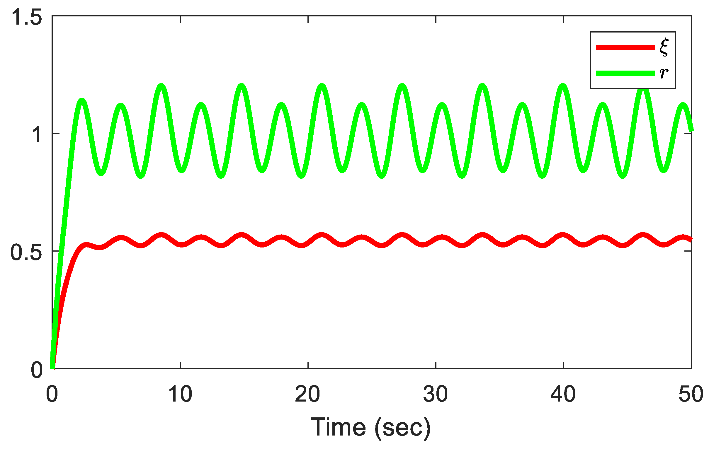
The performance of the proposed adaptive control scheme is evaluated through the simulation results shown in Figure 2, Figure 3, Figure 4, Figure 5, Figure 6 and Figure 7. Figure 2 compares the system output y with the desired reference signal , from which it can be observed that the output accurately follows the reference trajectory, demonstrating satisfactory tracking behavior. The corresponding tracking error is shown in Figure 3, where it is seen to gradually decrease and remain confined within a small region near the origin, indicating successful achievement of the tracking objective. Figure 4 illustrates the time response of the state variable . The results indicate that stays within acceptable bounds throughout the simulation interval, which supports the stability of the closed loop system. The evolution of the estimated parameters and is presented in Figure 5. Their bounded and well behaved trajectories confirm the capability of the adaptive laws to compensate for parametric uncertainties. The control input u together with the delayed signal is shown in Figure 6. Both signals vary smoothly over time, demonstrating that the input delay does not induce oscillations or destabilizing effects. Finally, Figure 7 depicts the unmodeled dynamics and r, which remain bounded during the entire simulation. Overall, these simulation outcomes verify that the proposed control framework ensures boundedness of all system signals while maintaining reliable and accurate tracking performance.
Example 2:
Consider a practical application involving a one-link robotic manipulator with motor dynamics, as investigated in [51]. The dynamic equations of the system are given by
where q, , and denote the link position, velocity, and acceleration, respectively. The variable I represents the generated motor torque, denotes the disturbance torque, and V is the electromechanical control input. The system parameters are chosen as , , , , , and . It is assumed that the system is subject to input delay and unmodeled dynamics. Define the state variables as , , , and the delayed control input as .
Then, the system (84) can be transformed as
where , , , , , , , , , and consequently . Additionally, the input delay is modeled by .
The reference trajectory is selected as . The initial states and parameter estimates are chosen as , , and , for . The design constants are set to , , , and .
The fuzzy logic systems employ Gaussian-type basis functions given by , , , where the indices satisfy .
Define the nonlinear functions as , , , and . Under these selections, Assumption 1 is satisfied. To fulfill Assumption 2, choose the Lyapunov candidate together with and . In accordance with Lemma 2, select , , , . Consequently, the auxiliary dynamic signal r evolves according to .
The first-step virtual controllers and are synthesized following the design in (54), while the real control signal u is generated in accordance with (69). The parameter estimation dynamics , and are specified by the update laws given in (55). The performance of the proposed adaptive control method is evaluated through the simulation results depicted in Figure 8, Figure 9, Figure 10, Figure 11, Figure 12 and Figure 13. Figure 8 presents the time responses of the system output y along with the desired reference signal , showing close agreement and indicating that the controller achieves precise output tracking. The associated tracking error is shown in Figure 9, where it gradually decreases and remains within a small neighborhood of the origin, confirming the successful achievement of the tracking objective. The temporal behaviors of the state variables and are illustrated in Figure 10, demonstrating that both states remain bounded over the entire simulation period, which validates the stability of the closed-loop system under the proposed controller. Figure 11 depicts the evolution of the estimated adaptive parameters , , and , whose bounded and smooth trajectories confirm the effectiveness of the adaptive laws in handling parametric uncertainties. Figure 12 compares the control input u with the delayed input , and the smooth variations of these signals indicate that input delays do not introduce instability or undesirable oscillations. Finally, Figure 13 shows the unmodeled dynamics and r, which remain bounded throughout the simulation, further illustrating the robustness of the proposed approach. Collectively, these simulation results demonstrate that the developed control strategy ensures boundedness of all system signals while achieving accurate and reliable tracking performance.
5. Conclusions
This study has investigated the design of a predefined-time adaptive fuzzy control scheme for high-order nonlinear systems with nonstrict-feedback structures, considering the presence of unmodeled dynamics and input delays. To compensate for the effects of unmodeled dynamics, a predefined-time auxiliary dynamic signal was incorporated, while the impact of input delays was alleviated using a Padé approximation in conjunction with an intermediate variable. Fuzzy logic systems were utilized to approximate the unknown nonlinear functions, thereby reducing reliance on an accurate mathematical model of the system. By integrating the recursive backstepping technique with a power-type Lyapunov function framework, an adaptive fuzzy predefined-time tracking controller was developed. A comprehensive analytical study establishes that the designed feedback dynamics ensure practical predefined-time convergence of the closed-loop system, while suitable adjustment of the controller gains confines the tracking deviations within a small vicinity of the equilibrium point. The effectiveness and advantages of the proposed control strategy were further validated through simulation examples. Future research will focus on extending the proposed predefined-time adaptive fuzzy control framework to more complex system classes, such as switched stochastic nonlinear systems. In such systems, random disturbances, stochastic uncertainties, and switching behaviors coexist, posing significant challenges to stability analysis and controller design. Incorporating predefined-time performance guarantees under stochastic effects and switching signals, while accounting for unmodeled dynamics and input delays, remains an open and meaningful research direction. Additionally, event-triggered mechanisms and network-induced constraints will be considered to improve communication efficiency and practical implementability in large-scale and distributed control systems.
Author Contributions
Mohamed Kharrat : Writing – original draft, Supervision, Paolo Mercorelli: Writing – review & editing. All authors have read and agreed to the published version of the manuscript.
Data Availability Statement
No data were used for the research described in the article.
Conflicts of Interest
The authors declare no conflicts of interest.
References
- Zhang, Y.; Ning, X.; Wang, Z.; Yu, D. High-order disturbance observer-based neural adaptive control for space unmanned systems with stochastic and high-dynamic uncertainties. IEEE Access 2021, 9, 77028–77043. [Google Scholar] [CrossRef]
- Kharrat, M.; Mercorelli, P. Neural Network-Based Adaptive Finite-Time Control for Pure-Feedback Stochastic Nonlinear Systems with Full State Constraints, Actuator Faults, and Backlash-like Hysteresis. Mathematics 2025, 14, 30. [Google Scholar] [CrossRef]
- Cui, Y.; Duan, G.; Liu, X.; Zheng, H. Adaptive fuzzy fault-tolerant control of high-order nonlinear systems: A fully actuated system approach. Int. J. Fuzzy Syst. 2023, 25, 1895–1906. [Google Scholar] [CrossRef]
- Sui, S.; Chen, C. P.; Tong, S. Finite-time adaptive fuzzy prescribed performance control for high-order stochastic nonlinear systems. IEEE Trans. Fuzzy Syst. 2021, 30, 2227–2240. [Google Scholar] [CrossRef]
- Deng, C.; Wen, C.; Wang, W.; Li, X.; Yue, D. Distributed adaptive tracking control for high-order nonlinear multiagent systems over event-triggered communication. IEEE Trans. Autom. Control 2022, 68, 1176–1183. [Google Scholar] [CrossRef]
- Duan, G. High-order fully actuated system approaches: Part IV. Adaptive control and high-order backstepping. Int. J. Syst. Sci. 2021, 52, 972–989. [Google Scholar] [CrossRef]
- Hou, M.; Shi, W.; Fang, L.; Duan, G. Adaptive dynamic surface control of high-order strict feedback nonlinear systems with parameter estimations. Sci. China Inf. Sci. 2023, 66, 159203. [Google Scholar] [CrossRef]
- Liu, S.; Niu, B.; Zong, G.; Zhao, X.; Xu, N. Adaptive neural dynamic-memory event-triggered control of high-order random nonlinear systems with deferred output constraints. IEEE Trans. Autom. Sci. Eng. 2023, 21, 2779–2791. [Google Scholar] [CrossRef]
- Niu, Y.; Yang, Y.; Wang, H.; Niu, B.; Shang, Z. Adaptive tracking control of high-order nonlinear systems with time-varying delays under asymmetric output constraints. IEEE Trans. Autom. Sci. Eng. 2024, 22, 2020–2030. [Google Scholar] [CrossRef]
- Kharrat, M.; Paolo, M. Predefined-Time Adaptive Command Filter Control for Nonstrict-Feedback Nonlinear Systems with Input Delay and Unmodeled Dynamics. Mathematics 2025, 14, 14. [Google Scholar] [CrossRef]
- Shi, X.; Xu, S.; Jia, X.; Chu, Y.; Zhang, Z. Adaptive neural control of state-constrained MIMO nonlinear systems with unmodeled dynamics. Nonlinear Dyn. 2022, 108, 4005–4020. [Google Scholar] [CrossRef]
- Wang, H.; Liu, P. X.; Li, S.; Wang, D. Adaptive neural output-feedback control for a class of nonlower triangular nonlinear systems with unmodeled dynamics. IEEE Trans. Neural Networks Learn. Syst. 2017, 29, 3658–3668. [Google Scholar] [CrossRef]
- Jiang, Z. P.; Praly, L. Design of robust adaptive controllers for nonlinear systems with dynamic uncertainties. Automatica 1998, 34, 825–840. [Google Scholar] [CrossRef]
- Sui, S.; Chen, C. P.; Tong, S. Event-trigger-based finite-time fuzzy adaptive control for stochastic nonlinear system with unmodeled dynamics. IEEE Trans. Fuzzy Syst. 2020, 29, 1914–1926. [Google Scholar] [CrossRef]
- Lyu, Z.; Liu, Z.; Xie, K.; Chen, C. P.; Zhang, Y. Adaptive fuzzy output-feedback control for switched nonlinear systems with stable and unstable unmodeled dynamics. IEEE Trans. Fuzzy Syst. 2019, 28, 1825–1839. [Google Scholar] [CrossRef]
- Shen, Q.; Shi, P.; Wang, S.; Shi, Y. Fuzzy adaptive control of a class of nonlinear systems with unmodeled dynamics. Int. J. Adapt. Control Signal Process. 2019, 33, 712–730. [Google Scholar] [CrossRef]
- Tong, S.; Li, Y. Adaptive fuzzy output feedback control for switched nonlinear systems with unmodeled dynamics. IEEE Trans. Cybern. 2016, 47, 295–305. [Google Scholar] [CrossRef] [PubMed]
- Zhang, L.; Wang, P.; Hua, C. Adaptive control of time-delay nonlinear HOFA systems with unmodeled dynamics and unknown dead-zone input. Int. J. Robust Nonlinear Control 2023, 33, 2615–2628. [Google Scholar] [CrossRef]
- Bi, W. Neural networks adaptive control for fractional-order non-linear system with unmodelled dynamics and actuator faults. IET Control Theory Appl. 2023, 17, 259–269. [Google Scholar] [CrossRef]
- Sui, S.; Chen, C. P.; Tong, S. Event-trigger-based finite-time fuzzy adaptive control for stochastic nonlinear system with unmodeled dynamics. IEEE Trans. Fuzzy Syst. 2020, 29, 1914–1926. [Google Scholar] [CrossRef]
- Hua, Y.; Zhang, T. Adaptive control of pure-feedback nonlinear systems with full-state time-varying constraints and unmodeled dynamics. Int. J. Adapt. Control Signal Process. 2020, 34, 183–198. [Google Scholar] [CrossRef]
- Li, D. P.; Liu, Y. J.; Tong, S.; Chen, C. P.; Li, D. J. Neural networks-based adaptive control for nonlinear state constrained systems with input delay. IEEE Trans. Cybern. 2018, 49, 1249–1258. [Google Scholar] [CrossRef]
- Deng, W.; Yao, J.; Ma, D. Adaptive control of input delayed uncertain nonlinear systems with time-varying output constraints. IEEE Access 2017, 5, 15271–15282. [Google Scholar] [CrossRef]
- Zhao, J.; Tong, S.; Li, Y. Observer-based fuzzy adaptive control for MIMO nonlinear systems with non-constant control gain and input delay. IET Control Theory Appl. 2021, 15, 1488–1505. [Google Scholar] [CrossRef]
- Wang, Y.; Zhang, J.; Zhang, H.; Xie, X. Adaptive fuzzy output-constrained control for nonlinear stochastic systems with input delay and unknown control coefficients. IEEE Trans. Cybern. 2020, 51, 5279–5290. [Google Scholar] [CrossRef]
- Han, Y. Q. Design of decentralized adaptive control approach for large-scale nonlinear systems subjected to input delays under prescribed performance. Nonlinear Dyn. 2021, 106, 565–582. [Google Scholar] [CrossRef]
- Li, Z.; Li, T.; Feng, G.; Zhao, R.; Shan, Q. Neural network-based adaptive control for pure-feedback stochastic nonlinear systems with time-varying delays and dead-zone input. IEEE Trans. Syst. Man, Cybern. Syst. 2018, 50, 5317–5329. [Google Scholar] [CrossRef]
- Qi, X.; Liu, W.; Lu, J. Observer-based finite-time adaptive prescribed performance control for nonlinear systems with input delay. Int. J. Control. Autom. Syst. 2022, 20, 1428–1438. [Google Scholar] [CrossRef]
- Han, Y. Q.; He, W. J.; Li, N.; Zhu, S. L. Adaptive tracking control of a class of nonlinear systems with input delay and dynamic uncertainties using multi-dimensional Taylor network. Int. J. Control. Autom. Syst. 2021, 19, 4078–4089. [Google Scholar] [CrossRef]
- Zhu, B.; Karimi, H. R.; Zhang, L.; Zhao, X. Neural network-based adaptive reinforcement learning for optimized backstepping tracking control of nonlinear systems with input delay. Appl. Intell. 2025, 55, 129. [Google Scholar] [CrossRef]
- Zheng, X. Y. Adaptive neural control for non-strict feedback stochastic nonlinear systems with input delay. Trans. Inst. Meas. Control 2024, 46, 104–115. [Google Scholar] [CrossRef]
- Kharrat, M. Finite-Time Fuzzy Adaptive Control for Nonlinear Systems With Asymmetric Dead-Zone and Actuator Faults and via an Event-Triggered Mechanism. International Journal of Adaptive Control and Signal Processing 2025. [Google Scholar] [CrossRef]
- Kharrat, M. Neural Network-Based Adaptive Finite-Time Command-Filter Control for Nonlinear Systems With Input Delay and Input Saturation. Int. J. Adapt. Control Signal Process. 2025, 39, 231–243. [Google Scholar]
- Kharrat, M. Fixed-Time Adaptive Tracking Control for Nonlinear Systems With Unmodeled Dynamics and Input Dead-Zone and Saturation. International Journal of Robust and Nonlinear Control 2025. [Google Scholar] [CrossRef]
- Kharrat, M. Adaptive fixed-time command-filtered funnel control for nonstrict-feedback nonlinear systems with input saturation. Transactions of the Institute of Measurement and Control 2025, 01423312251361970. [Google Scholar] [CrossRef]
- Kharrat, M.; Alhazmi, H. Fixed-time adaptive control for nonstrict-feedback nonlinear systems with sensor faults and input saturation. J. Low Freq. Noise, Vib. Act. Control 2025, 44, 565–587. [Google Scholar] [CrossRef]
- Kharrat, M.; Alhazmi, H. Fixed-Time Adaptive Control for Nonstrict-Feedback Nonlinear Systems with Input Delay and Unknown Backlash-Like Hysteresis. Neural Process. Lett. 2025, 57, 52. [Google Scholar] [CrossRef]
- Kharrat, M. Predefined-time adaptive fuzzy control for nonlinear cyber-physical systems under sensor and actuator attacks. Journal of Vibration and Control 2025, 10775463251374117. [Google Scholar] [CrossRef]
- Zhao, L.; Sui, S.; Chen, C. P. Adaptive Predefined-Time Control for High-Order Nonlinear Systems With Unmodeled Dynamics. International Journal of Adaptive Control and Signal Processing 2025. [Google Scholar] [CrossRef]
- Sui, S.; Chen, C. P.; Tong, S. Command filter-based predefined time adaptive control for nonlinear systems. IEEE Trans. Autom. Control 2024, 69, 7863–7870. [Google Scholar] [CrossRef]
- Wang, H.; Tong, M.; Zhao, X.; Niu, B.; Yang, M. Predefined-time adaptive neural tracking control of switched nonlinear systems. IEEE Trans. Cybern. 2022, 53, 6538–6548. [Google Scholar] [CrossRef] [PubMed]
- Zhang, Y.; Chadli, M.; Xiang, Z. Predefined-time adaptive fuzzy control for a class of nonlinear systems with output hysteresis. IEEE Trans. Fuzzy Syst. 2022, 31, 2522–2531. [Google Scholar] [CrossRef]
- Xu, H.; Yu, D.; Liu, Y. J. Observer-based fuzzy adaptive predefined time control for uncertain nonlinear systems with full-state error constraints. IEEE Trans. Fuzzy Syst. 2023, 32, 1370–1382. [Google Scholar] [CrossRef]
- Chen, P.; Tan, J.; Yao, Y.; Zhang, X.; Yao, Y. Predefined-time adaptive fuzzy control for nonlinear systems with input saturation and deferred restriction. Nonlinear Dyn. 2025, 113, 4727–4744. [Google Scholar] [CrossRef]
- Yang, Y.; Sui, S.; Chen, C. P. Adaptive predefined time control for stochastic switched nonlinear systems with full-state error constraints and input quantization. IEEE Transactions on Cybernetics, 2025. [Google Scholar]
- Wang, L.; Xin, M.; Niu, J. Adaptive fuzzy predefined-time control for stochastic nonlinear systems against actuator and sensor faults. IEEE Transactions on Instrumentation and Measurement, 2025. [Google Scholar]
- Sui, S.; Zhao, L.; Chen, C. P. Adaptive fuzzy predefined-time tracking control design for nonstrict-feedback high-order nonlinear systems with input quantization. IEEE Trans. Fuzzy Syst. 2024, 32, 5978–5990. [Google Scholar] [CrossRef]
- Ling, S.; Wang, H.; Liu, P. X. Adaptive tracking control of high-order nonlinear systems under asymmetric output constraint. Automatica 2020, 122, 109281. [Google Scholar] [CrossRef]
- Cui, D.; Xiang, Z. Nonsingular fixed-time fault-tolerant fuzzy control for switched uncertain nonlinear systems. IEEE Trans. Fuzzy Syst. 2022, 31, 174–183. [Google Scholar] [CrossRef]
- Wu, Y.; Xie, X. J.; Hou, Z. G. Adaptive fuzzy asymptotic tracking control of state-constrained high-order nonlinear time-delay systems and its applications. IEEE Trans. Cybern. 2020, 52, 1671–1680. [Google Scholar] [CrossRef]
- Zhai, J.; Wang, H.; Tao, J.; He, Z. Observer-based adaptive fuzzy finite time control for non-strict feedback nonlinear systems with unmodeled dynamics and input delay. Nonlinear Dyn. 2023, 111, 1417–1440. [Google Scholar] [CrossRef]
Figure 1.
Block diagram depicting the structure of the developed control architecture.
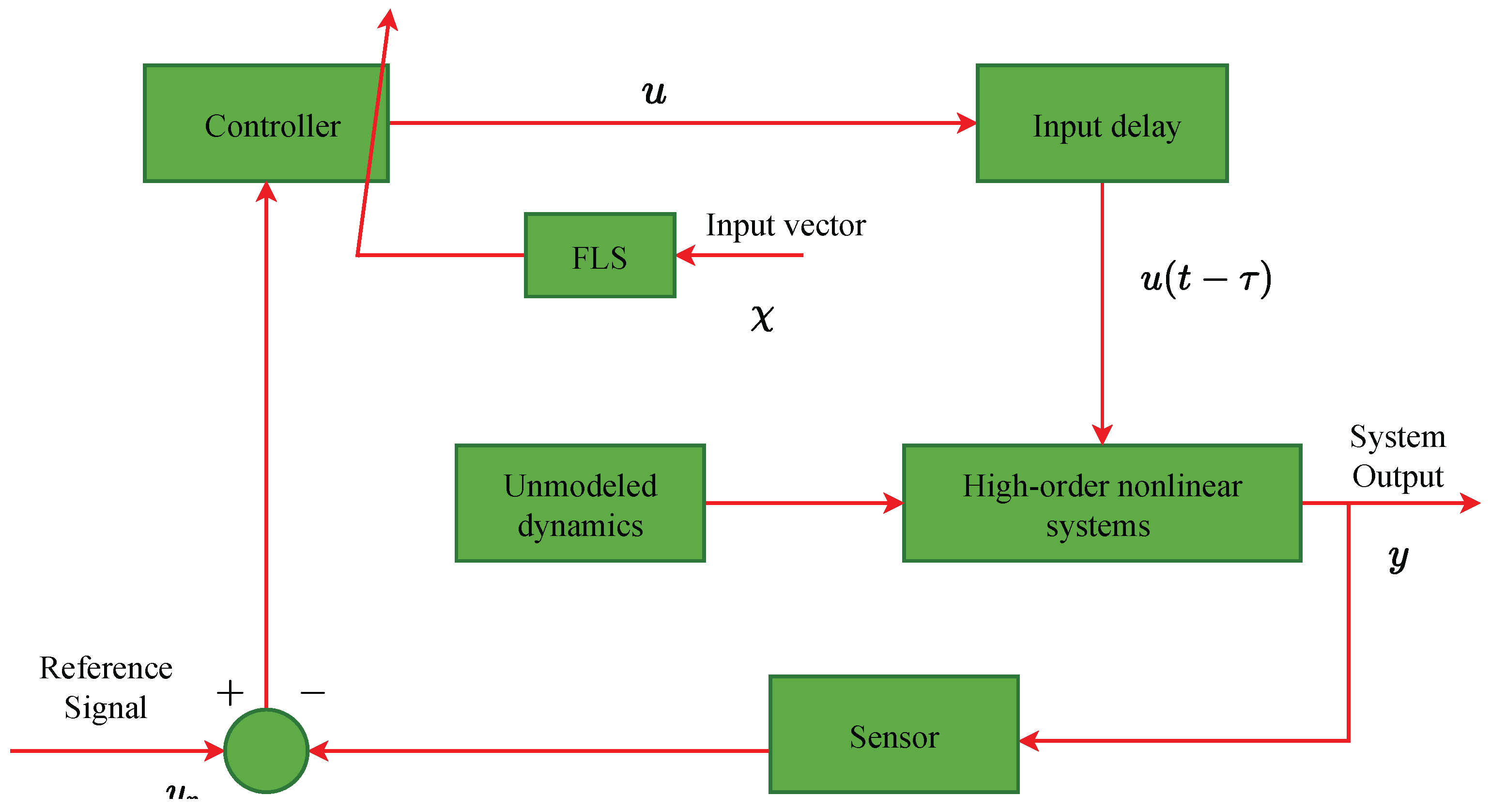
Figure 2.
Trajectories of y and .
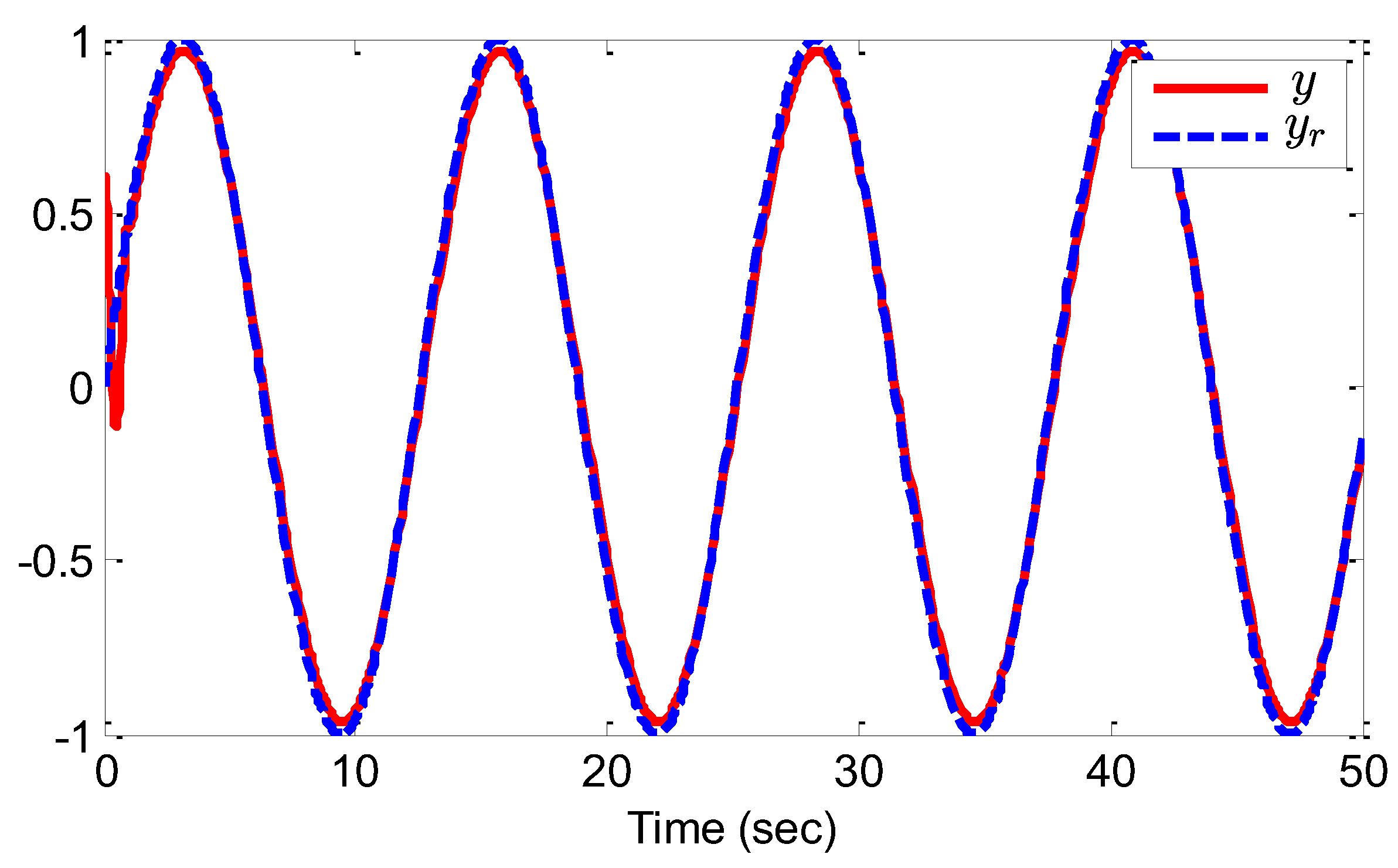
Figure 3.
The trajectory of the tracking error .
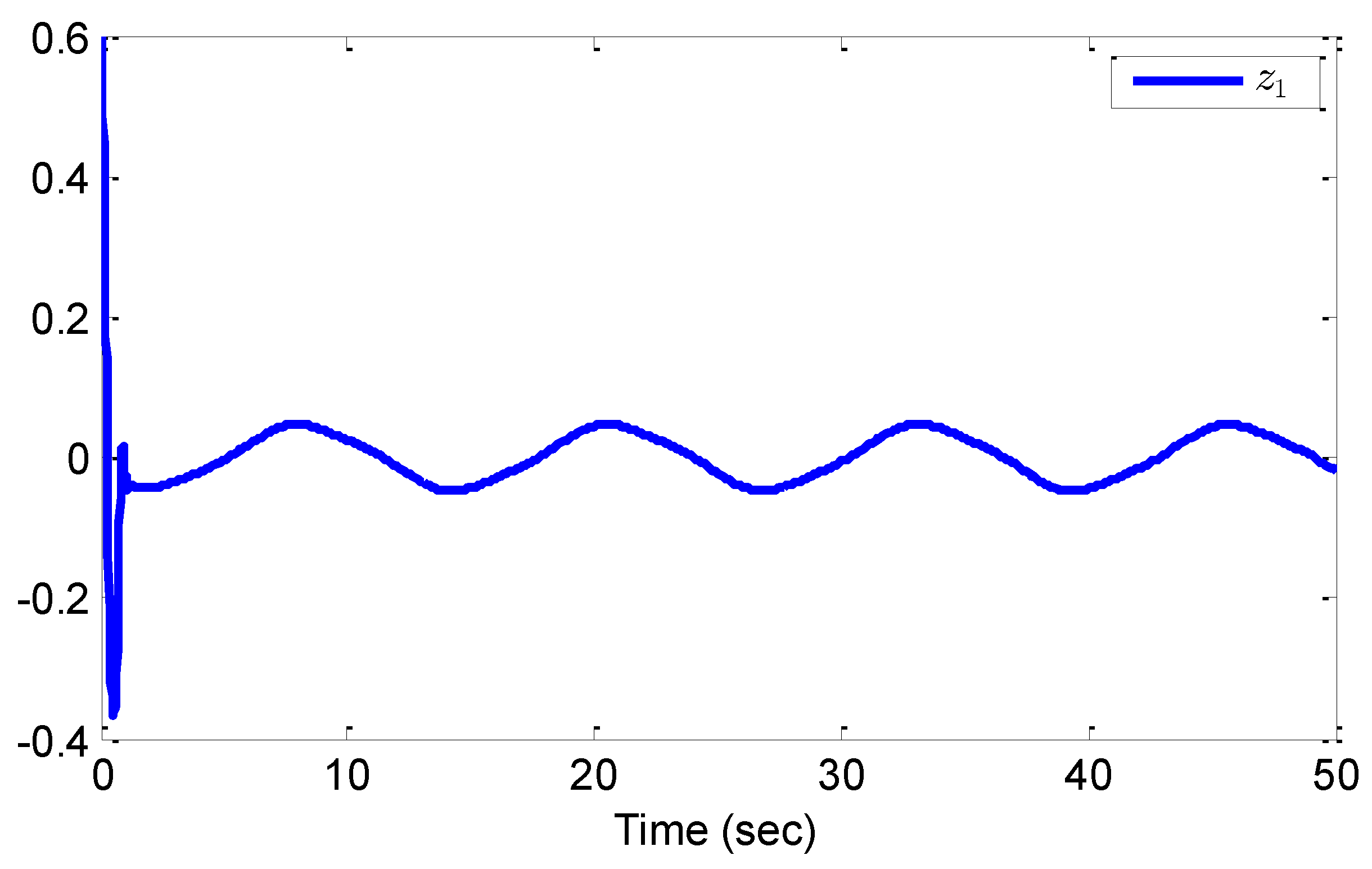
Figure 4.
State variables .
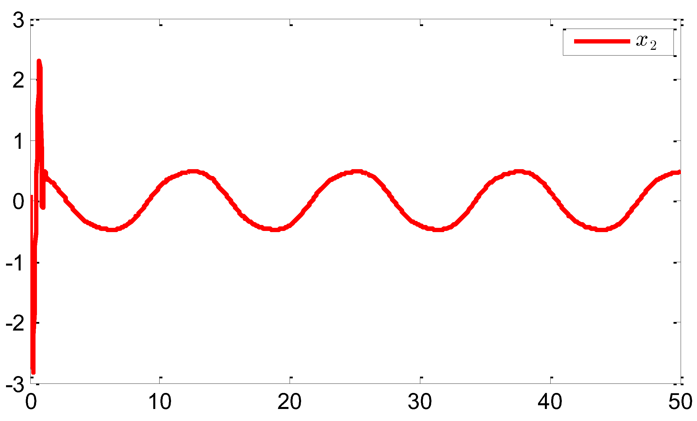
Figure 5.
Adaptive laws and .
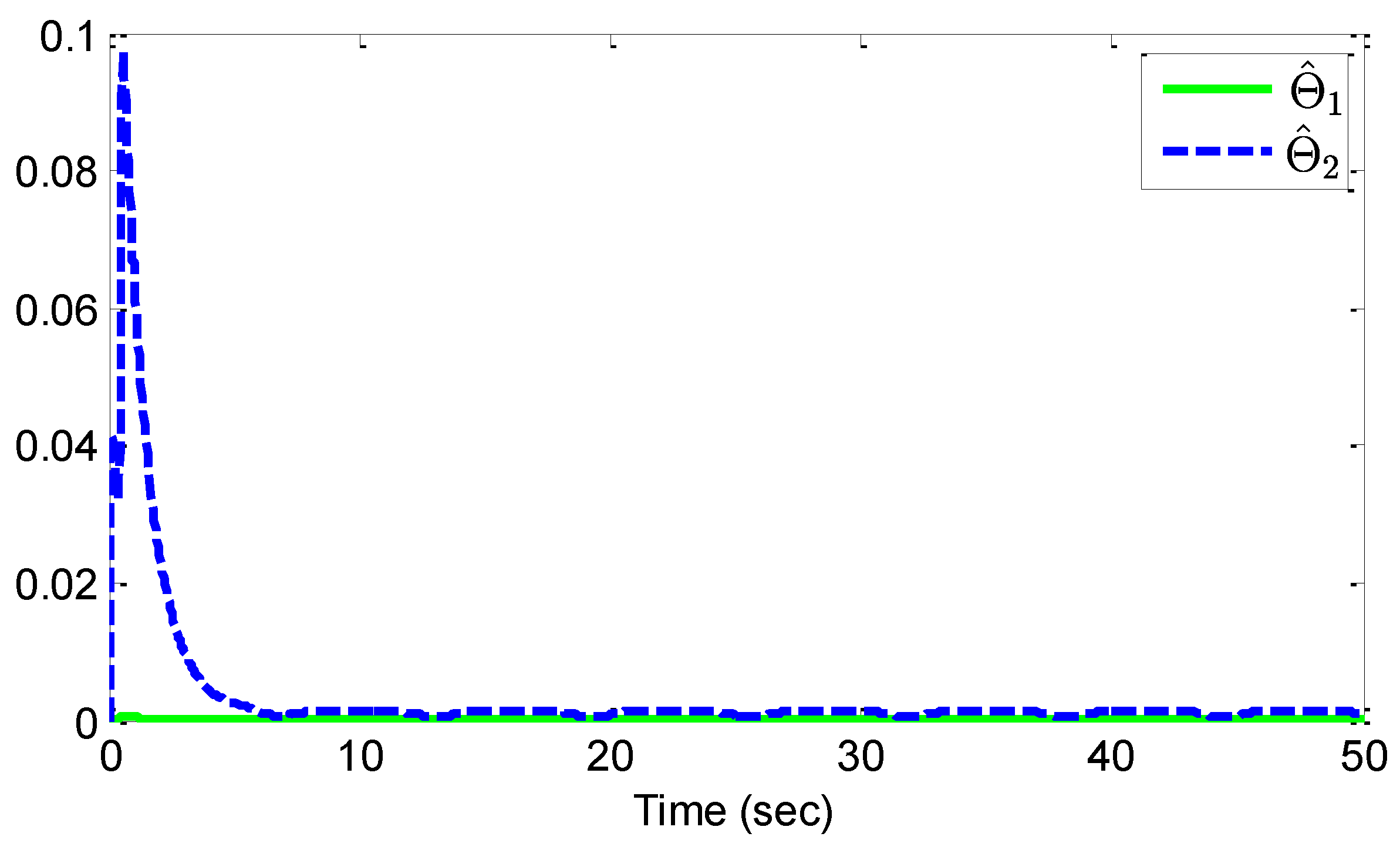
Figure 6.
System input and control input u.
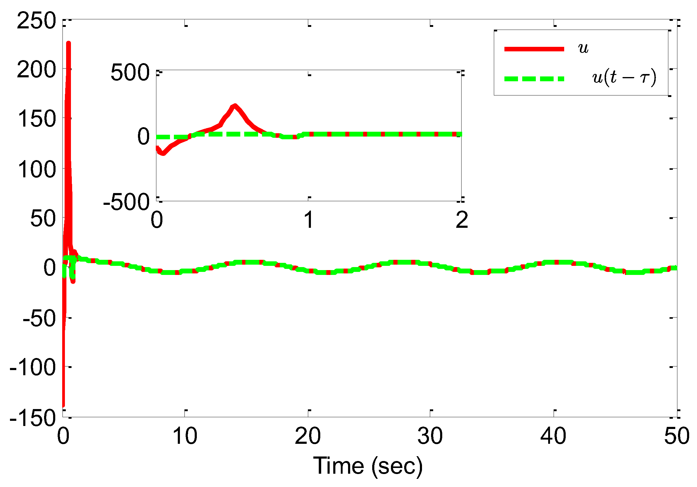
Figure 7.
Trajectories of and r.
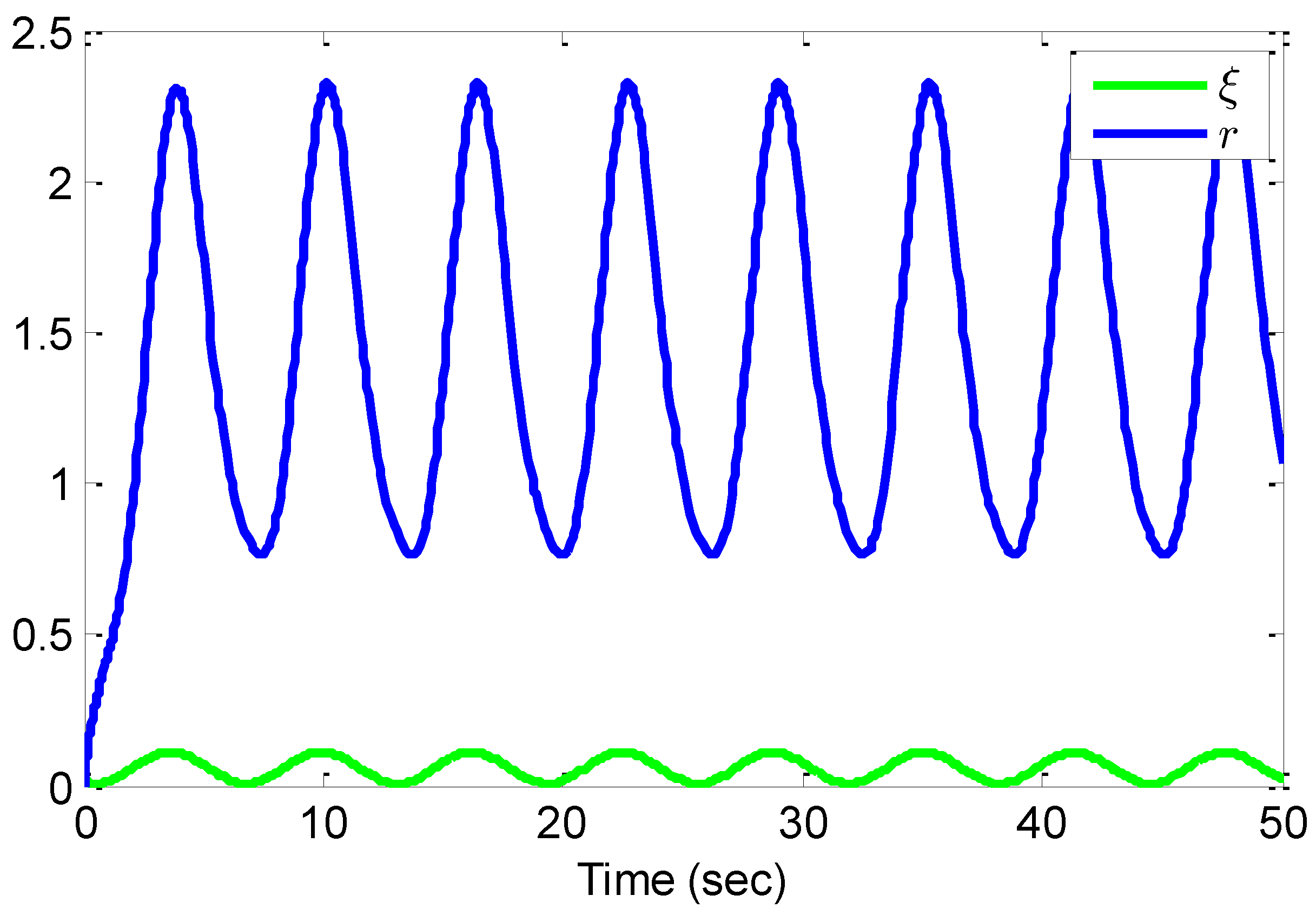
Figure 8.
Trajectories of y and .
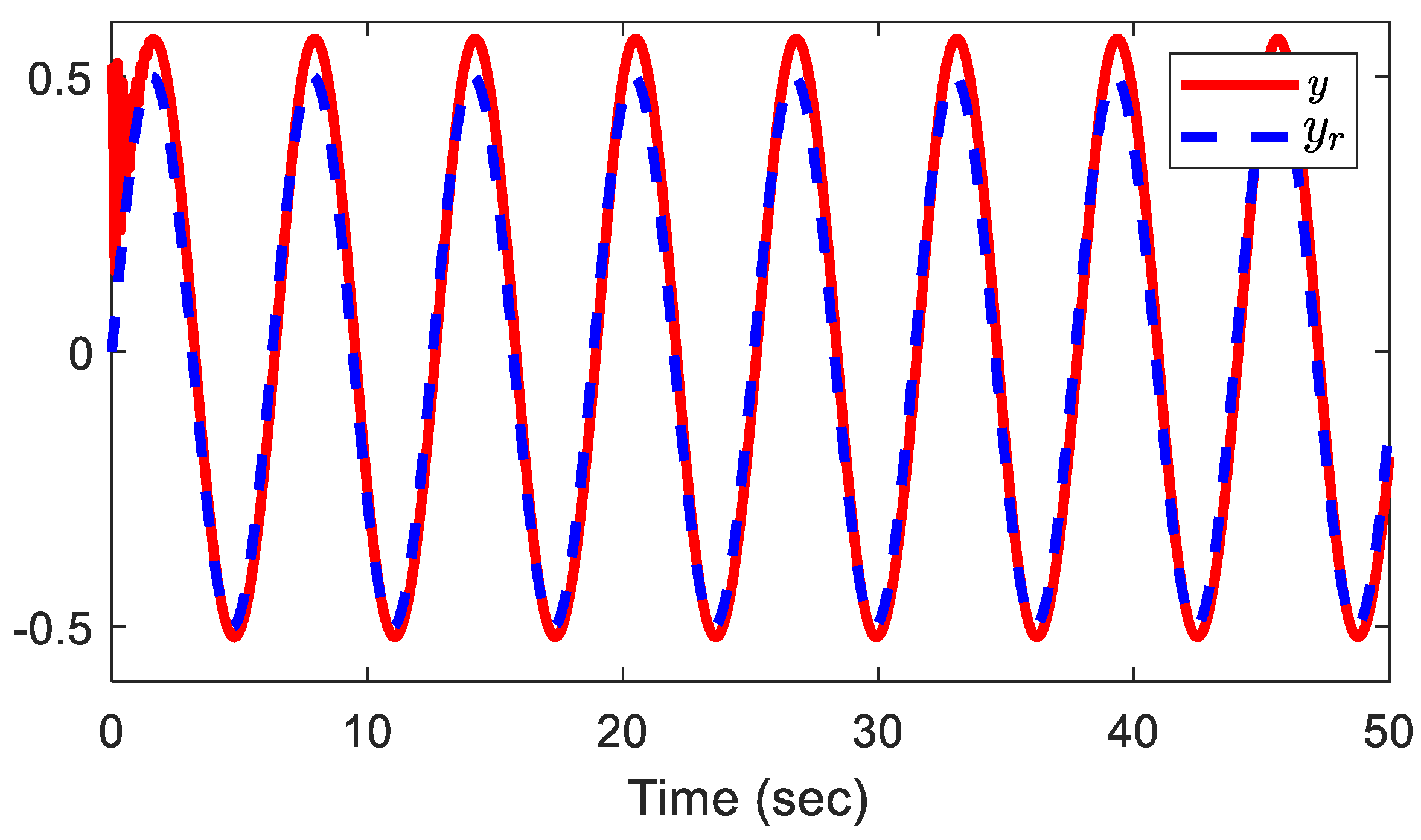
Figure 9.
The trajectory of the tracking error .
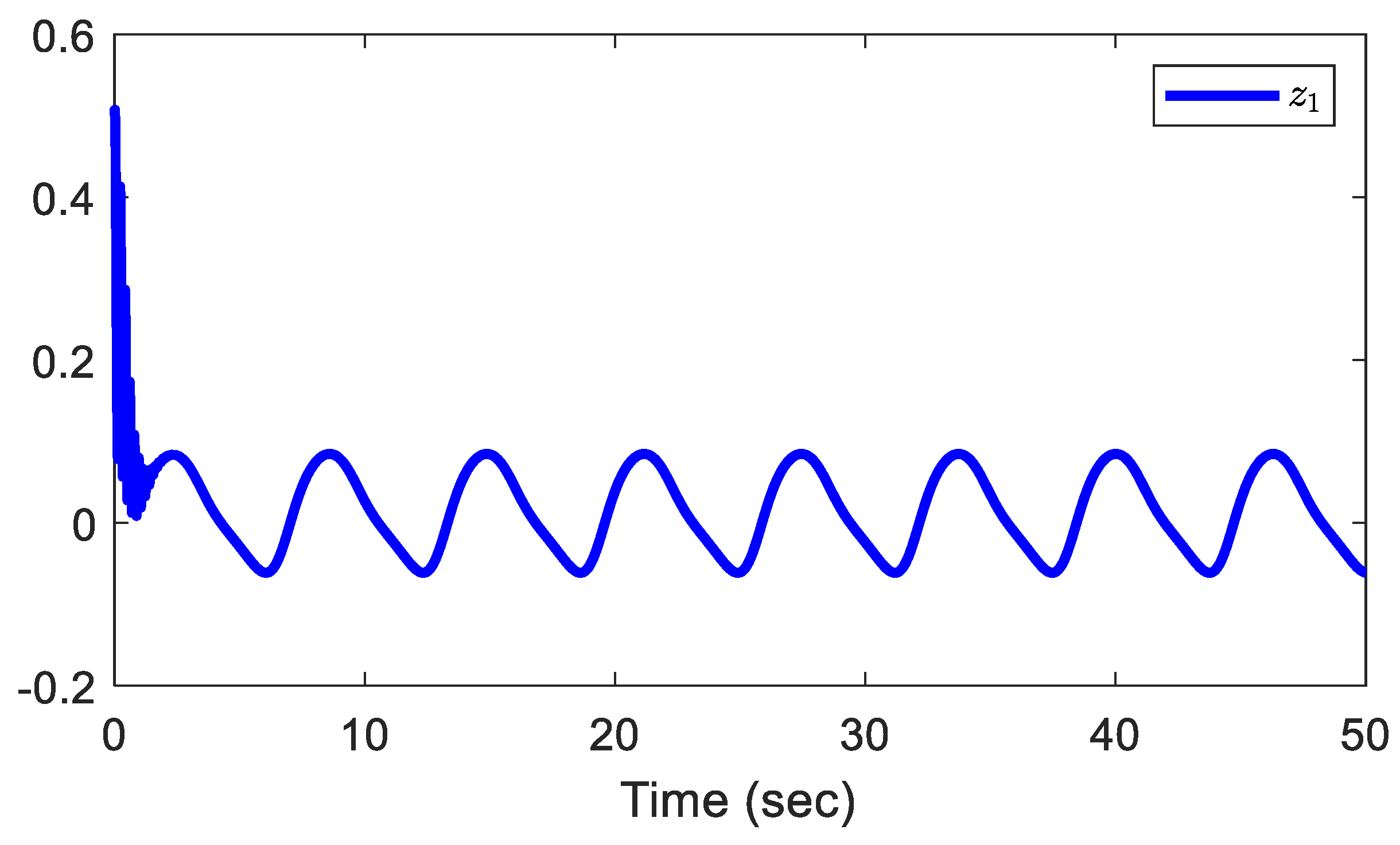
Figure 10.
State variables and .
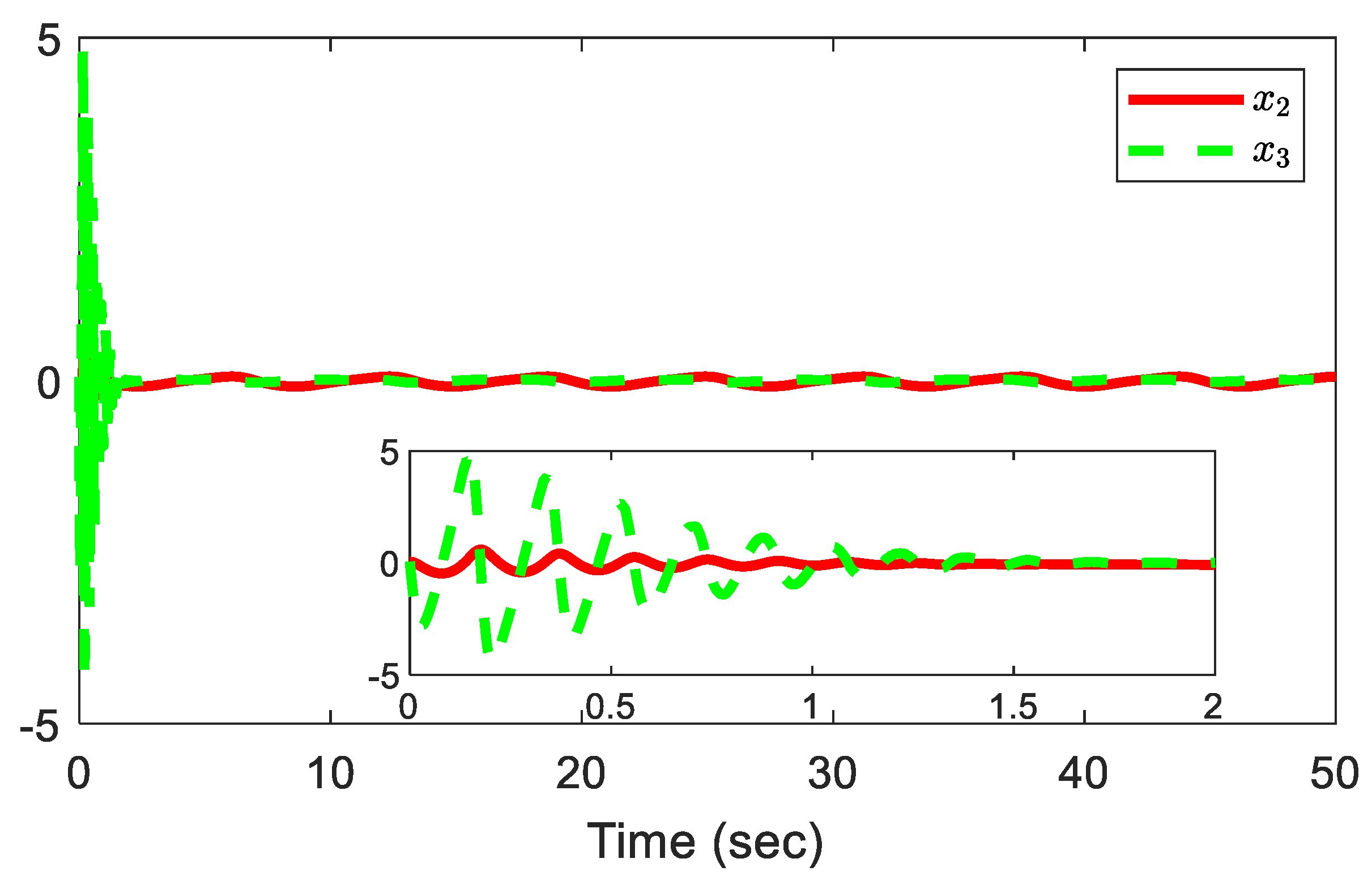
Figure 11.
Adaptive laws , , and .
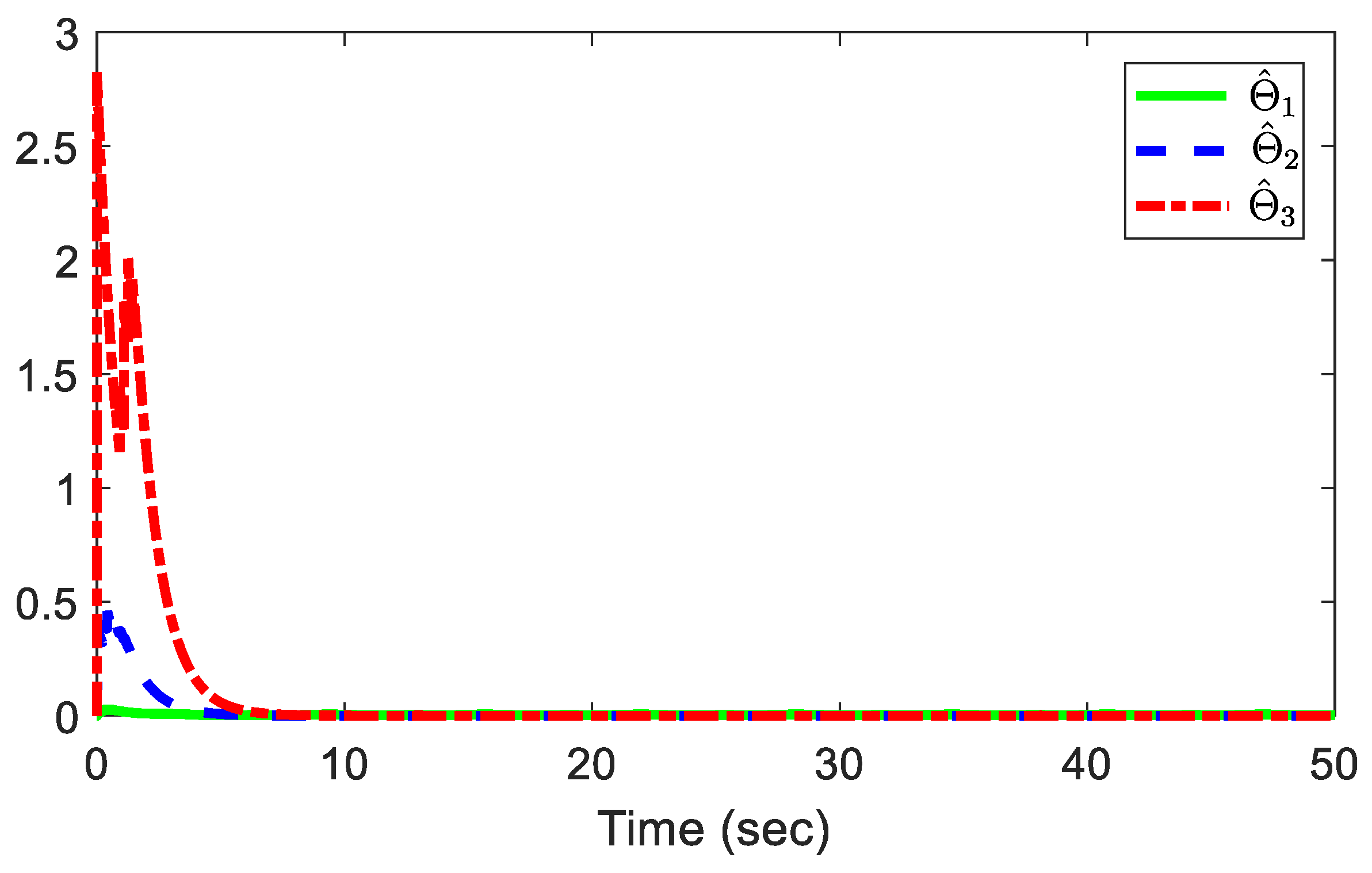
Figure 12.
Control input u and system input .
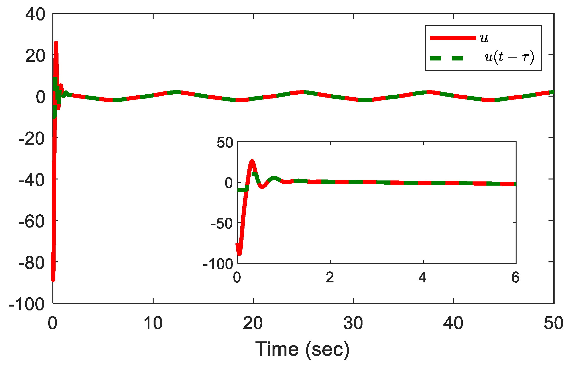
Figure 13.
Trajectories of and r.
Disclaimer/Publisher’s Note: The statements, opinions and data contained in all publications are solely those of the individual author(s) and contributor(s) and not of MDPI and/or the editor(s). MDPI and/or the editor(s) disclaim responsibility for any injury to people or property resulting from any ideas, methods, instructions or products referred to in the content. |
© 2026 by the authors. Licensee MDPI, Basel, Switzerland. This article is an open access article distributed under the terms and conditions of the Creative Commons Attribution (CC BY) license (http://creativecommons.org/licenses/by/4.0/).
Copyright: This open access article is published under a Creative Commons CC BY 4.0 license, which permit the free download, distribution, and reuse, provided that the author and preprint are cited in any reuse.


