Submitted:
30 January 2026
Posted:
02 February 2026
You are already at the latest version
Abstract
Radio-frequency (RF) antenna design traditionally proceeds in three phases. First, the design performance is modeled with expensive, proprietary software. Second, the design is built using precision metal machining or printed circuit board (PCB) fabrication. Third, the result is characterized using RF measurement tools. The process can include machine learning for optimization. We have developed an open-source alternative process that utilizes the MIT Electromagnetic Equation Propagator (MEEP) package for design and simulation, and open-source 3D printing with conductive polymer for fabrication. Using this process, we designed and fabricated a broadband RF horn antenna. The $\mathbf{E}$-plane and $\mathbf{H}$-plane radiation patterns, the VSWR, and the cross-polarization match MEEP calculations. These results indicate that our design is a linearly polarized, broadband RF horn antenna in the [5.5-6] GHz bandwidth. Though our data are limited to frequencies $\leq 6$ GHz, our MEEP calculations predict good performance above 6 GHz. Future work will include expanding the bandwidth with larger RF structures, and constructing a broadband RF phased array.
Keywords:
Computational Electromagnetism (CEM)
; additive manufacturing
; MEEP
; RF engineering
; open-source design
1. Introduction
Broadband RF antennas are ubiquitous tools within scientific instrumentation and communications. Traditionally, these are designed with expensive, proprietary software packages [1,2]. Designs are fabricated by cutting metal with precision machine tools (subtractive manufacturing). Compared to additive manufacturing techniques, subtractive manufacturing can be costly for rapid prototyping [3,4]. Open-source additive manufacturing boosts cost efficiency in both the design and fabrication, provided the 3D printing filament has sufficient conductivity.
Development of new RF antenna designs requires exploration of conductor shapes that set the boundary conditions for radiated signals. Developing new shapes that meet design requirements has been aided by machine learning (ML) strategies [5,6,7]. While mixing new ML algorithms into open CEM code is straightforward, incorporating them into proprietary software is often challenging. Ideally, RF engineers would keep the functionality of proprietary software, while retaining the flexibility to incorporate new ML techniques. Creating a design process based on open CEM tools achieves this goal.
Previously, J. C. Hanson (2021) demonstrated that the open-source MEEP software package may be used as an RF antenna design tool [8]. MEEP operates via the FDTD algorithm for Maxwell’s Equations on a Yee lattice [9]. The key to the technique is that MEEP is written to account for the scale-invariance of Maxwell’s Equations. Even though MEEP is tradiationally used for designs with wavelengths at the m scale, designs in with wavelengths at the cm scale may be created scaling length units within MEEP. Specifically, J. C. Hanson produced RF phased array designs in two and three dimensions using MEEP functionality [8]. The designs included broadband RF horn elements in the [0.5-5] GHz bandwidth. Further, J. C. Hanson demonstrated that open-source CAD software may be used to create complex designs that can be 3D printed [10].
In recent years, RF antenna systems have begun to be fabricated with 3D printing. The authors of [11] presented a hybrid strategy that combined traditional PCB fabrication, non-conductive 3D printing, and metallization of 3D printed structures. The assembled structure was a low-cost, electronically steerable MIMO array for mm-Wave 5G applications. The authors of [12] produced a waveguide-fed holographic beam-forming antenna using a dual print-head 3D printing system that combined non-conductive PLA supports with conductive filament. The result was a steerable beam at frequencies near 10 GHz. The authors of [13] produced a Mills-Cross, frequency-diverse, metasurface antenna capable of electronic steering in the K-band, using a mixture of non-conductive PLA and conductive filament. Finally, the authors of [14] printed a holgraphic metasurface antenna using the same technique found in [13] for Fresnel-zone focusing on and off-axis in the X-band.
In this work, we present the first open-source, broadband, 3D printed RF horn, designed with MEEP and fabricated entirely from conductive 3D-printer filament. In Sec. Section 2, we explain the open-source design, CAD, and fabrication techniques. In Sec. Section 3, we show that the -plane and -plane radiation patterns, the VSWR, and the cross-polarization ratios match predictions. In Sec. Section 4, we discuss the limitations of our analysis, summarize key results, and discuss applications and future directions for this research.
2. Methods and Materials
The goal of this work was to use open CEM tools to design, model, and fabricate a linearly polarized, broadband RF horn antenna in the multi-GHz bandwidth. Over the past decade, MEEP has most often been used to design photonics systems [15,16]. Recently, MEEP has been used to model electromagnetic propagation with wavelengths at the cm-scale [8,10]. Further, antenna designs created with open CAD tools like kLayout can be imported into MEEP. Using parametric CAD design, we can specify antenna shapes using analytic functions that are then translated into kLayout and MEEP. Designs in kLayout can also be translated into 3D printer files, ensuring the device and model match.
Our open fabrication technique hinges on the existence of commerically available conductive 3D printer filament. Multi3D1 has shown that a copper-doped thermoplastic serves as a 3D printer filament with resistivities of cm, depending on the printing pattern. Using a tungsten-tipped 3D printing head and Electrifi filament from Multi3D, we can complete antenna prints with volumes of in several hours. The printed structures are fitted with RF connectors and tested as receivers on custom mounts, while using a network analyzer connected to a log-periodic dipole array (LPDA) antenna as the transmitter. Figure 1 (left) contains a diagram of the design and fabrication process.
2.1. CEM Design and Open-Source CAD
The kLayout design of the RF horn is shown in Figure 1 (right). The open-source CEM design begins with choosing parametric design parameters for the exponential RF horn. The horn cavity is the rectangular volume where the coaxial cable attaches. The horn surfaces are the curved structures that connect the cavity to open space. The opening is the area where the surfaces stop and radiation exits the horn. Let the origin of an coordinate system refer to the center of the left edge of the cavity in Figure 1 (right). Let refer to the cavity length in the x-direction, refer to the cavity width in the y-direction, refer to the surface length in the x-direction, and w refer to the opening width in the y-direction. Using these variables, Equations 1 and specify the shape of the RF horn surfaces in the -plane:
The function in Equation 1 describes the upper surface in Figure 1, while describes the lower surface. Table 1 contains the values for , , , and w corresponding to our first 3D printed RF horn. The horn is designed to be linearly polarized in the y-direction. When we are performing calculations in 3D with MEEP, we give the RF horn a height z, out of the page in Figure 1 (right).
In previous studies [8], antenna structures were instantiated as native MEEP objects. For example, the following Python3 code with the Meep library imported as mp adds N 2D exponential horns to the overall geometry via the mp.Block() method:
for j in range(0,n_antenna):
y = j*d_y+y0
#Describe the cavity
cav_back_location = mp.Vector3(x0,y)
cav_location_pos = mp.Vector3(c_l/2.0+x0,c_w/2.0+y)
cav_location_neg = mp.Vector3(c_l/2.0+x0,-c_w/2.0+y)
backplate = mp.Block(backplate_size,center=cav_back_location,material=mp.metal)
cav_upper = mp.Block(side_plate_size,center=cav_location_pos,material=mp.metal)
cav_lower = mp.Block(side_plate_size,center=cav_location_neg,material=mp.metal)
geometry.append(cav_upper)
geometry.append(cav_lower)
geometry.append(backplate)
#Describe the horn surfaces
size_upper = mp.Vector3(dx,thickness)
size_lower = mp.Vector3(dx,thickness)
for i in range(0,n_slices):
center_upper = mp.Vector3(i*dx+c_l+x0,c_w/2*np.exp(k*(i*dx-c_l))+y)
center_lower = mp.Vector3(i*dx+c_l+x0,-c_w/2*np.exp(k*(i*dx-c_l))+y)
geometry.append(mp.Block(size_upper,center=center_upper,material=mp.metal))
geometry.append(mp.Block(size_lower,center=center_lower,material=mp.metal))
With appropriate constants defined, this code creates a one-dimensional phased array of 2D RF horns with MEEP conductors. There are two advantages to this parametric design: it is fast and simple to code, and no other tools or programs outside of MEEP are required. Structures can be quickly modified by exploring the parameter space defined by the constants in Tab. Table 1. The disadvantage is that complex structures must be assembled from simple ones with little visualization and a large high-performance computing (HPC) memory usage. Using open CAD programs like kLayout, however, antenna structures are designed visually and imported into MEEP.
This procedure relies adept coordination between MEEP and kLayout. First, we create a list of the vertices of the antenna structures using Python3 functions evaluating Eqs. 1- and other simple pouints for the cavity. Second, we create placeholder polygons in kLayout. Third, we copy the vertices into the kLayout polygons. This procedure results in 2D structures like those shown in Figure 1 (right). Figure 1 (right) is a design of the RF horn in the -plane. We give the design a height in the z-direction after importing to MEEP. MEEP accepts GDSII files produced by kLayout, which can also be converted to STL files suitable for 3D printing software. In practice, free tools like the educational version of AutoDesk Inventor are useful for fine-tuning designs.
2.1.1. Radiation Pattern Calculations
We compute the antenna radiation pattern in MEEP using near-to-far field projection2. First, a NearToFarRegion is created to fully enclose the structure, similar to a Gaussian surface in classical electrodynamics. Second, the get_farfield() function computes the and fields a distance r from the origin after the sim.run() function completes. In Figure 1, the -plane is the -plane, and the -plane is the -plane. We chose meters, given the dimensions of the horn (Tab. Table 1) and cm wavelengths. Third, we compute the normalized Poynting vector along the and -planes. The following code produces the normalized -plane radiation pattern, with MEEP as mp, NumPy as np, and proj_box as the NearToFarRegion:
def calculate_E_plane_rad_patt(sim,proj_box):
r = 1000
npts = 360
E = np.zeros((npts,3),dtype=np.complex128)
H = np.zeros((npts,3),dtype=np.complex128)
angles = 2*np.pi/npts*np.arange(npts)
for n in range(npts):
x = r*np.cos(angles[n])
y = r*np.sin(angles[n])
ff = sim.get_farfield(proj_box,mp.Vector3(x,y,0))
E[n,:] = [ff[j] for j in range(3)]
H[n,:] = [ff[j+3] for j in range(3)]
Px = np.real(np.conj(E[:,1])*H[:,2]-np.conj(E[:,2])*H[:,1])
Py = np.real(np.conj(E[:,2])*H[:,0]-np.conj(E[:,0])*H[:,2])
Pr = np.sqrt(np.square(Px) + np.square(Py))
directivity = 10.0*np.log10(Pr/max(Pr))
return (angles,directivity)
To obtain the radiation pattern, the sim.run() command must be executed such that sufficient radiation has passed through the NearToFarField region.
2.1.2. VSWR Calculations
The voltage standing wave radio (VSWR) is a standard RF figure of merit. The VSWR may be expressed in terms of the complex reflection coefficient, , between coaxial line and RF antenna input port:
To calculate VSWR, we send a pulse signal down the simulated coaxial cable, and measure . This strategy is based on FluxRegion objects, similar to NearToFarRegion objects3.
Figure 2 (left) shows the upper left region of the RF horn CAD, depicting the radiation source within the structure representing the coaxial cable. The coaxial cable model is built from outer conductors, dielectric materials, and an inner conductor with a radiating source polarized radially. While the radiation pattern analysis uses a continuous-wave source, the source in our VSWR analysis is a custom pulse signal with a broadband spectrum. In the middle of the cable, a MEEP FluxRegion is created. The FluxRegion records electromagnetic flux through a geometric region, simular to a Gaussian surface in classical electrodynamics. Both FluxRegion and NearToFarRegion objects can record information at multiple frequencies. In our radiation pattern analysis, we set the NearToFarRegion frequency to the source frequency. In our VSWR analysis, we chose 1024 frequencies ranging from [0-10] GHz for the FluxRegion.
The reflection coefficient is measured in two stages. First, the MEEP simulation is run for a time corresponding to the length of the coaxial cable, accounting for the speed of propagation in the dielectric material. The simulation is reset, and the original flux is multiplied by and pre-loaded into the FluxRegion. The simulation is then run for a factor of 2 longer, so that any reflections from the antenna have time to reach the FluxRegion a second time. The FluxRegion records the reflected flux, having already cancelled the input flux from the pre-loaded negative input flux. Thus, using one FluxRegion, the ratio of reflected to input flux, , can be calculated. The VSWR is then derived from (Eq. 3).
2.2. Fabrication Technique
The 3D printed RF horn was fine-tuned with Autodesk Inventor with the free Education Plan. The equations that decribe the RF horn, Eqs. 1 and , can be implemented with the parameters in Tab. Table 1 using the Equation Curve feature. Inventor accepts parametric modeling, meaning parameters from Tab. Table 1 can be edited to produce new designs. Merging the mathematical form of Eqs. 1 and required parameterization into a format useable by the Equation Curve feature. Other challenges that are unique to this process involve maintaining geometric design constraints. Since adjusting parameters or design offsets may result in a design that violates a design constraint, the process required fine tuning.
The 3D print workflow requires careful consideration. The Multi3D Electrifi filament was found to be more difficult to print than PLA or PETG. The tall and narrow nature of the model produced issues with build plate adhesion. To address this, two steps were added to the workflow: glue from a glue stick or spray can was applied to a layer of masking tape on the print bed, and removable buttresses were added to the print structure. The filament was printed between 135-145 degrees C, and no bed heating was required. Our printer is a dual print-head Prusa XL, with a modified tungsten tipped nozzle to reduce abrasion. The slicing program used to translate from CAD to printer firmware was PrusaSlicer, which has a method for including custom firmware commands. Crucially, a custom command was required to allow the printer to print below its minimum safety temperature.
2.3. Computational Hardware
We performed our MEEP calculations on a System76 Thelio Major, with an AMD Ryzen Threadripper 3990X 64-core motherboard. This motherboard enables hyper-threading, so the effective number of cores is 128. With 256 GB of memory, the memory per core is 2 GB. The FDTD approach for CEM modeling is memory intensive, so it was important to equip the system with sufficient memory. In practice, memory consumption peaks at about 32 GB when running MEEP in parallel across 64 cores when computing a 3D radiation pattern using near-to-far field projection. The enhanced memory per core allows multiple users to create runs exploring different antenna parameters.
In Figure 3, the times required for set up and completion of a 2D version of the -plane radiation pattern calculation are shown versus number of parallel cores used. In Figure 3 (left), the data correspond to the set_epsilon function. This function sets the boundary conditions that result from structures imported from our open-source CAD. These calculations represent the majority of the time required to complete the run. The total run times are shown in Figure 3 (right). The times scale with the resolution parameter, used to set the number of pixels per unit area. The expectation for a 2D calculation is that set-up time or total time scales with resolution squared. This expectation is represented by the solid black lines in Figure 3. While additional cores can accelerate set up and total times, too many cores yield only marginal gains, and can even slow the computation. However, using 16 or 32 cores reduces total run time below the resolution-squared expectation.
3. Results
Using the techniques described in Sec. Section 2.2, we fabricated an RF horn with the parameters in Tab. Table 1. Figure 4 contains photos of the results. As listed in Tab. Table 1, the RF horn is 16.5 cm long (see ruler in Figure 4). The dimensions of the opening are 2.5 x 8.5 cm. The SMA connector is mounted to the cavity, with a coaxial pin extending into the chamber such that the initial radiation is linearly polarized. The radiation pattern measurements were made in a co-polarized S21 configuration, and VSWR measurements are made with respect to a 50 RF coaxial cable connected to the printed RF horn.
3.1. Radiation Patterns
To measure radiation patterns, we bolted the RF horn on a camera mount, and configured it as the receiver into a network analyzer with [0-6] GHz bandwidth (Figure 5). For a transmitter, we used a rear-fed log-periodic dipole array (LPDA). The network analyzer was calibrated with a short element, open element, and 50 terminator. After calibration, the S21 measurement mode was activated, and the cables were connected together to form a closed loop without the antennas. The measured S21 showed a 0 dB loss across the 6 GHz bandwidth. The receiver and transmitter where then inserted, and the S21 measured versus frequency. The transmitter power was set to maximum, 20 dBm, meaning no amplifier was necessary. The distance between transmitter and receiver varied between 1-2 meters. Received power was measured above the noise floor in the bandwidth [5.5-6] GHz
We first verified qualitatively that the S21 power varied appropriately with -plane angle, -plane angle, and co-polarization angle. Next, the receiver and transmitter were mounted in a vertically polarized configuration so that -plane angle could be measured with a smartphone level tool (Figure 5). The S21 power was measured versus -plane angle. Next, the antennas were mounted in a horizontally polarized configuration, so that -plane angle could be measured with the same smartphone tool. The S21 power was normalized to the maximum received power, when the -plane and -plane angles were 0 and 90 degrees, respectively. The results are shown in Figure 6.
The polar plot ranges from -26 dB to 1 dB, and the data is normalized to 0 dB. In the spherical coordinate system for an RF antenna radiating in the x-direction, linearly polarized in the y-direction, the -plane angle is the azimuthal angle as measured from the x-axis. Thus, in Figure 6 (left) the data and MEEP model peak at 0 dB when the angle is 0 degrees. There is good agreement between the MEEP model and the measured S21 power. In the same coordinate system, the zenith angle is the -plane angle. Thus, in Figure 6 (right) the data and MEEP model peak at 0 dB when the angle is 90 degrees. As with the -plane, there is good agreement between the MEEP model and S21 power.
3.2. The VSWR
To measure the VSWR of the RF horn, we bolted the RF horn to the camera mount, and configured it as the transmitter on the network analyzer. Once again, the network analyzer was calibrated on [0-6] GHz. After calibration, the S11 measurement mode was activated, and we verified that we measured 50 resistance in the bandwidth of interest. Finally, we extracted the S11 reflection coefficient in dB from the network analyzer. We took two additional post-processing steps. First, we converted S11 in dB to linear S11, and then to VSWR using Eq. 3. Second, we smoothed the data with an 11-point running average. We chose the 11-point filter to remain symmetric about the sample of interest (5 points to either side). Though the S11 fluctuated, the 11-point running average revealed a trend that matches results from MEEP modeling. The results are shown in Figure 7.
After the two-stage post-processing, the VSWR from MEEP modeling matched the measured VSWR once we shifted the measured VSWR down by a factor of 4. The reason for this is the impedance mismatch between the line impedance from the coaxial cable, and the load impedance from the RF horn. For example, if , and , then the VSWR is a factor of 4 higher than it would be if the antenna were matched to the line (). Though the measured fluctuated between 50-200 , after converting to VSWR and scaling the data, we find a match to the MEEP calculation. Two additional observations are important to note. First, our VSWR calculation in MEEP was performed in 2D. This makes the calculation simpler, but it is not necessary. Second, the bandwidth of the network analyzer was limited to 6 GHz. Though our measured data stops at 6 GHz in Figure 7, the simulated VSWR in Figure 7 predicts good performance above 6 GHz.
3.3. Cross-Polarization Ratios
The final measurement we performed was the cross-polarization ratio. The 3D printed RF horn and LPDA were arranged in the same S21 configuration that was used to measure the radiation patterns. The RF horn was the receiver, and bolted to the mount such that an inclinometer would measure cross-polarization angle. The prediction for the dependence of received power versus cross-polarization angle is known from optics and antenna theory. Let be the received power, be the transmitted power, and be the cross-polarization angle. These are related by
When normalized, the ratio in dB is equivalent to normalized S21. The results are shown in Figure 8, and show good agreement with Eq. 4. The prediction from Eq. 4 tends to negative infinity in dB. In this regime we find a cross-polarization ratio approaching -15 dB, which is comparable to most side-lobes in broadband RF antennas.
3.4. Future Work: Expansion of Bandwidth via Scaled Design
One limitation of our current 3D printed RF horn is measuring the lower edge of the bandwidth. While the data in Figure 7 show equally efficient performance between [4-6] GHz, in practice, measuring S21 below 5.5 GHz is challenging due to decreased SNR at lower frequencies. We have scaled our RF horn design by a factor of 2, and are currently completing our first prints of this larger device. The predicted VSWR is shown in Figure 9, along with the VSWR corresponding to the open RF cable model and no RF horn.
In Figure 9, the VSWR data from Figure 7 is again plotted, but the frequencies have been scaled down by a factor of 2, corresponding to the larger 3D print design. The MEEP simulation uses an identical CAD file that has been scaled accordingly in kLayout, using the Scale feature. The data again matches the simulation. The dashed line represents the VSWR result if the RF horn structure is removed, leaving only the original RF cable. Only radiation at the highest frequencies leaves the open cable to free space. The MEEP simulation shows that a larger model should have better performance at low frequencies, and that a bandwidth of [1-6] GHz is expected.
4. Conclusions
The goal of this research is to demonstrate a fully open-source design and fabrication process for broadband RF phased arrays. The elimination of proprietary design software and the introduction of versitile 3D printing with conductive filament enhances RF phased array production in two ways. First, gains in cost-efficiency arise from the use of open-source tools and printing techniques. Second, new designs can be realized through innovative additive manufacturing techniques, rather than relying on traditional metal machining. We made progress towards these goals by producing our first fully open-source, 3D printed, broadband, linearly polarized RF horn. This is one of the first examples of a 3D printed broadband RF element using no metallization or post-printing procedures [11,12,13,14].
In Sec. Section 2.1, we shared example code that creates a 2D version of our 3D model using MEEP objects. We also shared how radiation patterns are calculated using MEEP algorithms, and outlined how we calculate the VSWR. We have created and run full 3D versions of the MEEP code used to produce the design calculations on our parallel HPC system. For 3D CAD, we selected kLayout to create detailed models of the RF horn that can be imported as MEEP structures. In Sec. Section 2.2, we described how our kLayout designs are translated to AutoDesk Inventor (Free education version), and fed to our PrusaXL 3D printing system. By relying on parametric design, the modeled system is geometrically identical to the fabricated system, within the precision of the 3D printer (about 0.2 mm). The simulation results behave as expected, and can be modified by changing the parametric design parameters. In Sec. Section 2.3, we list the computational time requirements, showing the advantages and disadvantages of parallel MEEP calculations.
In Secs. Section 3.1, Section 3.2 and Section 3.3, we showed that the measured radiation patterns in the and planes, the smoothed VSWR data, and the cross-polarization data all match MEEP calculations and theoretical expectations. The natural direction of the work is to expand RF bandwidth by enlarging the RF horn design, and to explore and optimize alternate designs in MEEP. In Sec. Section 3.4, we predicted an expanded bandwith for our new, larger RF horn under fabrication. Finally, we seek to print a set of N identical broadband RF elements to form a broadband RF phased array, as envisioned in [8]. We hope to explore operating the broadband RF phased array in a multibeam mode, using complex broadband source signals.
Author Contributions
J. C. Hanson (JCH) conceived of the open-source design process, produced the MEEP calculations that led to the RF horn design, identified the conductive 3D printer filament, incorporated open-source CAD, and produced fully three-dimensional CEM models to compute the VSWR and radiation patterns for the fabricated designs. A. Wildanger (AW) sourced materials, and imported CAD designs into 3D printing format, and completed 3D prints to produce the designs. Together, JCH and AW collected data using the RF measurement tools. JCH used the data to show that the MEEP calculations match the lab measurements. AW is exploring new models to be printed, including larger RF horn models.
Funding
This work was supported by NEEC grant N00178-25-0001 through NSWC Corona. Any opinions, findings, and conclusions or recommendations expressed in this material are those of the author and do not necessarily reflect the views of NSWC Corona or the Department of the Navy.
Data Availability Statement
Code and other resources available at https://github.com/918particle/Antenna-MEEP-project.
Acknowledgments
We would like to express our heartfelt gratitude to the Director of Research, Sponsored Programs, and Special Projects Administration at Whittier College: Lisa Newton. Lisa helped us write a successful grant application to the NAVSEA Naval Engineering Education Consortium (NEEC) program, and to properly acquire lab equipment using the funds. We would also like to thank the former Vice President of Academic Affairs for Whittier College: Sal Johnston. Sal supported the creation of our Educational Partnership Agreement (EPA) between Whittier College and NSWC Corona, which further aided in the acquisition of lab equipment and engineering training from colleagues at NSWC Corona.
Conflicts of Interest
The authors declare no conflicts of interest.
Abbreviations
The following abbreviations are used in this manuscript:
| CEM | Computational Electromagnetism |
| HPC | High-Performance Computing |
| LPDA | Log-periodic Dipole Array |
| MEEP | MIT Electromagnetic Equation Propagator |
| NEEC | Naval Engineering Education Consortium |
| NSWC Corona | Naval Surface Warfare Center, Corona Division |
| RF | Radio-frequency |
| PLA | Polylactice Acid |
| PETG | Polyethylene Glycol |
References
- 1. Ansys HFSS: Best-In-Class 3D High Frequency Structure Simulation Software. https://www.ansys.com/products/electronics/ansys-hfss. Accessed: 2025-12-02.
- XFdtd Software for 3D Electromagnetic Simulation. 02 12 2025. Available online: https://www.remcom.com/xfdtd-3d-em-simulation-software.
- Segovia-Guerrero, L.; Baladés, N.; Gallardo-Galán, J.J.; Gil-Mena, A.J.; Sales, D.L. Additive vs. Subtractive Manufacturing: A Comparative Life Cycle and Cost Analyses of Steel Mill Spare Parts. Journal of Manufacturing and Materials Processing 2025, 9, 138. [Google Scholar] [CrossRef]
- Additive Manufacturing vs. Subtractive Manufacturing: A Cost-Benefit Analysis. 02 12 2025. Available online: https://plentifulchoices.com/production-line/additive-manufacturing-cost.
- Gajbhiye, P.A.; Singh, S.P.; Sharma, M.K. A comprehensive review of AI and machine learning techniques in antenna design optimization and measurement. Discover Electronics 2025, 2, 46. [Google Scholar] [CrossRef]
- Goudos, S.K.; Kalialakis, C.; Mittra, R. Evolutionary Algorithms Applied to Antennas and Propagation: A Review of State of the Art. International Journal of Antennas and Propagation 2016, 2016, 1–12. [Google Scholar] [CrossRef]
- Linden, D.; Altshuler, E. Evolving wire antennas using genetic algorithms: a review. In Proceedings of the First NASA/DoD Workshop on Evolvable Hardware; 1999; pp. 225–232. [Google Scholar] [CrossRef]
- Hanson, J.C. Broadband RF Phased Array Design with MEEP: Comparisons to Array Theory in Two and Three Dimensions. Electronics 2021, 10, 415. [Google Scholar] [CrossRef]
- Oskooi, A.F.; Roundy, D.; Ibanescu, M.; Bermel, P.; Joannopoulos, J.; Johnson, S.G. Meep: A flexible free-software package for electromagnetic simulations by the FDTD method. Computer Physics Communications 2010, 181, 687–702. [Google Scholar] [CrossRef]
- MeepCon Broadband RF Phased Array Design with MEEP, MIT. MIT, 2022.
- Alkaraki, S.; Gao, Y. mm-Wave Low-Cost 3D Printed MIMO Antennas With Beam Switching Capabilities for 5G Communication Systems. IEEE Access 2020, 8, 32531–32541. [Google Scholar] [CrossRef]
- Yoo, I.; Gollub, J.; Ye, S.; Gray, A.; Yurduseven, O.; Deshpande, M.D.; Smith, D.R. Hollow Rectangular Waveguide-fed Holographic Beamforming Antenna Additively Manufactured (3D Printed) with Conductive Polymer. arXiv 2022, 2208.14531. [Google Scholar] [CrossRef]
- Yurduseven, O.; Flowers, P.; Ye, S.; Marks, D.L.; Gollub, J.N.; Fromenteze, T.; Wiley, B.J.; Smith, D.R. Computational microwave imaging using 3D printed conductive polymer frequency-diverse metasurface antennas. IET Microwaves, Antennas & Propagation 2017, 11, 1962–1969. [Google Scholar] [CrossRef]
- Yurduseven, O.; Ye, S.; Fromenteze, T.; Wiley, B.J.; Smith, D.R. 3D Conductive Polymer Printed Metasurface Antenna for Fresnel Focusing. Designs 2019, 3, 46. [Google Scholar] [CrossRef]
- Hammond, A.M.; Oskooi, A.; Chen, M.; Lin, Z.; Johnson, S.G.; Ralph, S.E. High-performance hybrid time/frequency-domain topology optimization for large-scale photonics inverse design. Optics Express 2022, 30, 4467. [Google Scholar] [CrossRef] [PubMed]
- Majumder, A.; Shen, B.; Polson, R.; Menon, R. Ultra-compact nanophotonic devices designed by computational metamaterials. Imaging and Applied Optics 2017 (3D, AIO, COSI, IS, MATH, pcAOP) 2017, p. IM2E.2. [Google Scholar] [CrossRef]
| 1 | |
| 2 | |
| 3 |
Figure 1.
(Left) Flow diagram for the open-source design and fabrication process. (Right) The kLayout CAD design for the RF horn (top view), with a coaxial cable attached. The x-direction is to the right, the y-direction is up, and the z-direction is out of the page. The white ruler gives 16.741 cm.
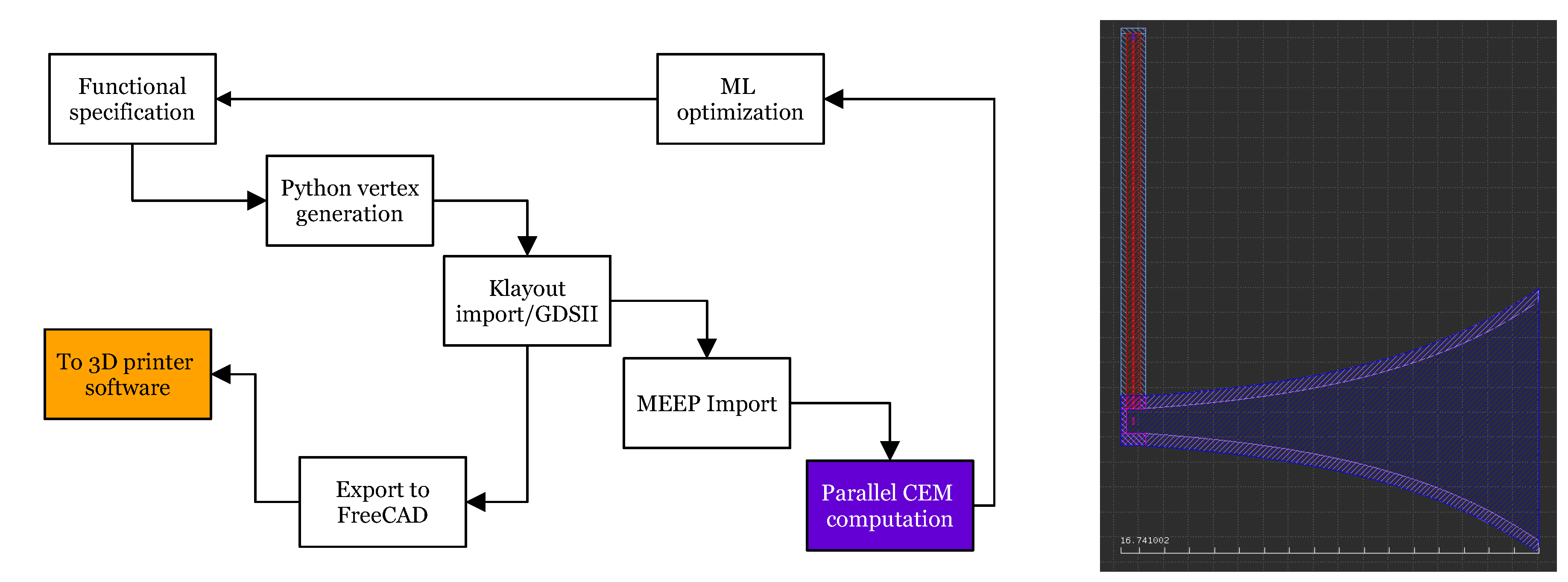
Figure 2.
(Left) The upper left region of Figure 1. The purple region is the radiating source used for VSWR analysis, the red regions are dielectric material, and the light blue regions are conductors. The combined structure represents a coaxial cable. (Right) The lower left region of Figure 1. The coaxial cable reaches the horn cavity, shown in light blue. The dark blue regions are the beginning of the horn surfaces. The pink structure in the center is the radiation source used for radiation pattern analysis.
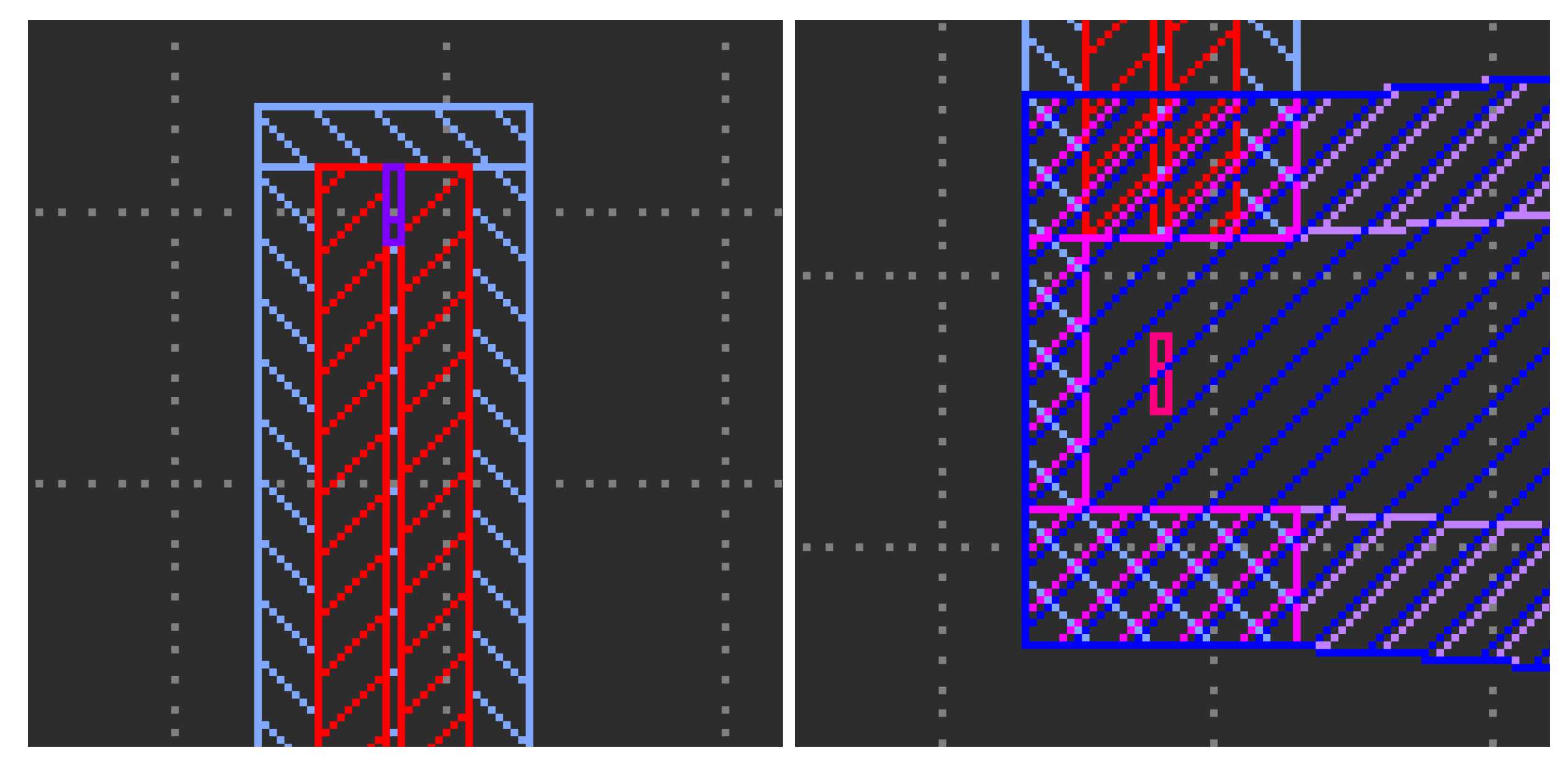
Figure 3.
(Left) Time (seconds) required to set boundary conditions in MEEP. (Right) Same as (left), to complete the run in MEEP, including near-to-far projection. Circles: resolution set to 10. Squares: resolution set to 20. Lines: resolution 10 data, scaled up by a factor of 4.
Figure 3.
(Left) Time (seconds) required to set boundary conditions in MEEP. (Right) Same as (left), to complete the run in MEEP, including near-to-far projection. Circles: resolution set to 10. Squares: resolution set to 20. Lines: resolution 10 data, scaled up by a factor of 4.
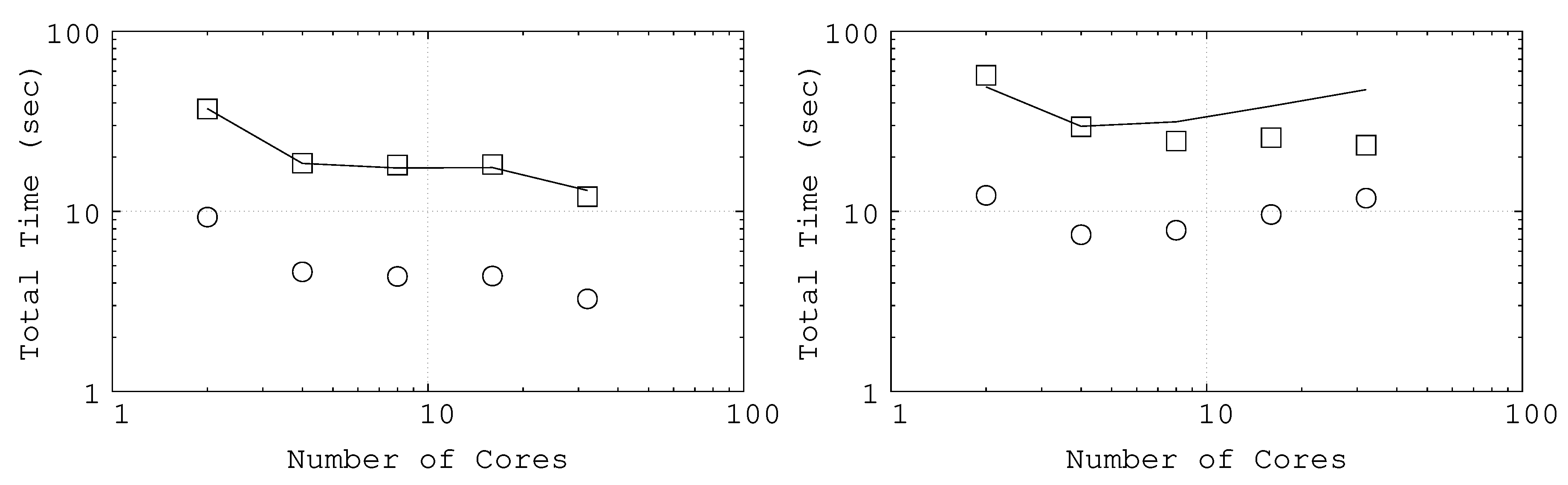
Figure 4.
(Left) The Prusa XL 3D printer beginning a print with the Electrifi filament. (Middle) The finished RF horn with SMA connector. (Right) The finished RF horn viewed with opening visible.
Figure 4.
(Left) The Prusa XL 3D printer beginning a print with the Electrifi filament. (Middle) The finished RF horn with SMA connector. (Right) The finished RF horn viewed with opening visible.
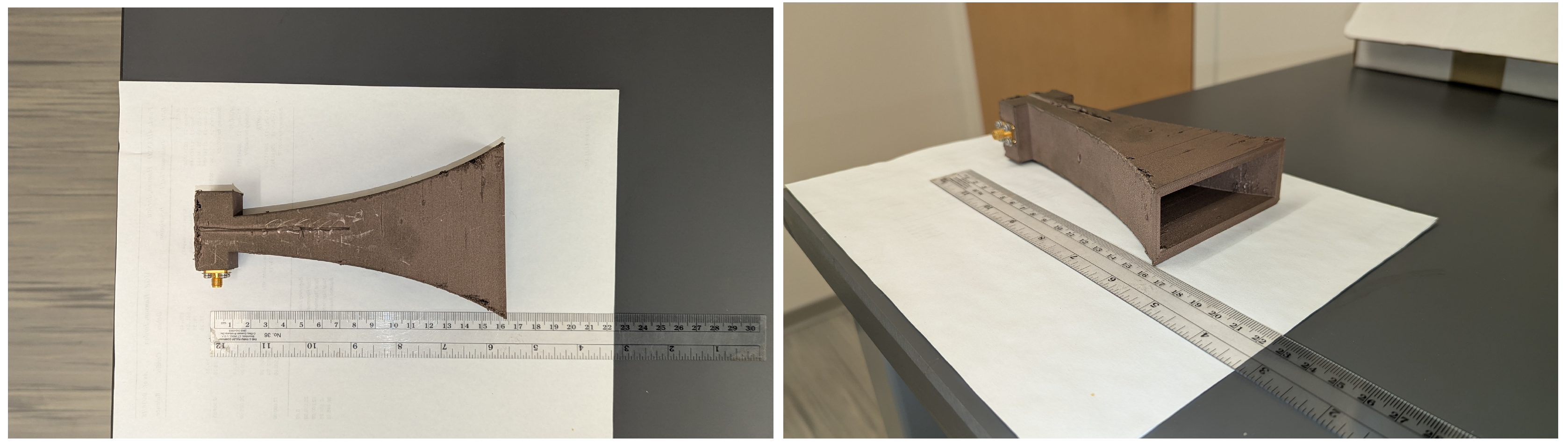
Figure 5.
The co-polarized configuration to measure the radiation pattern of the printed RF horn.
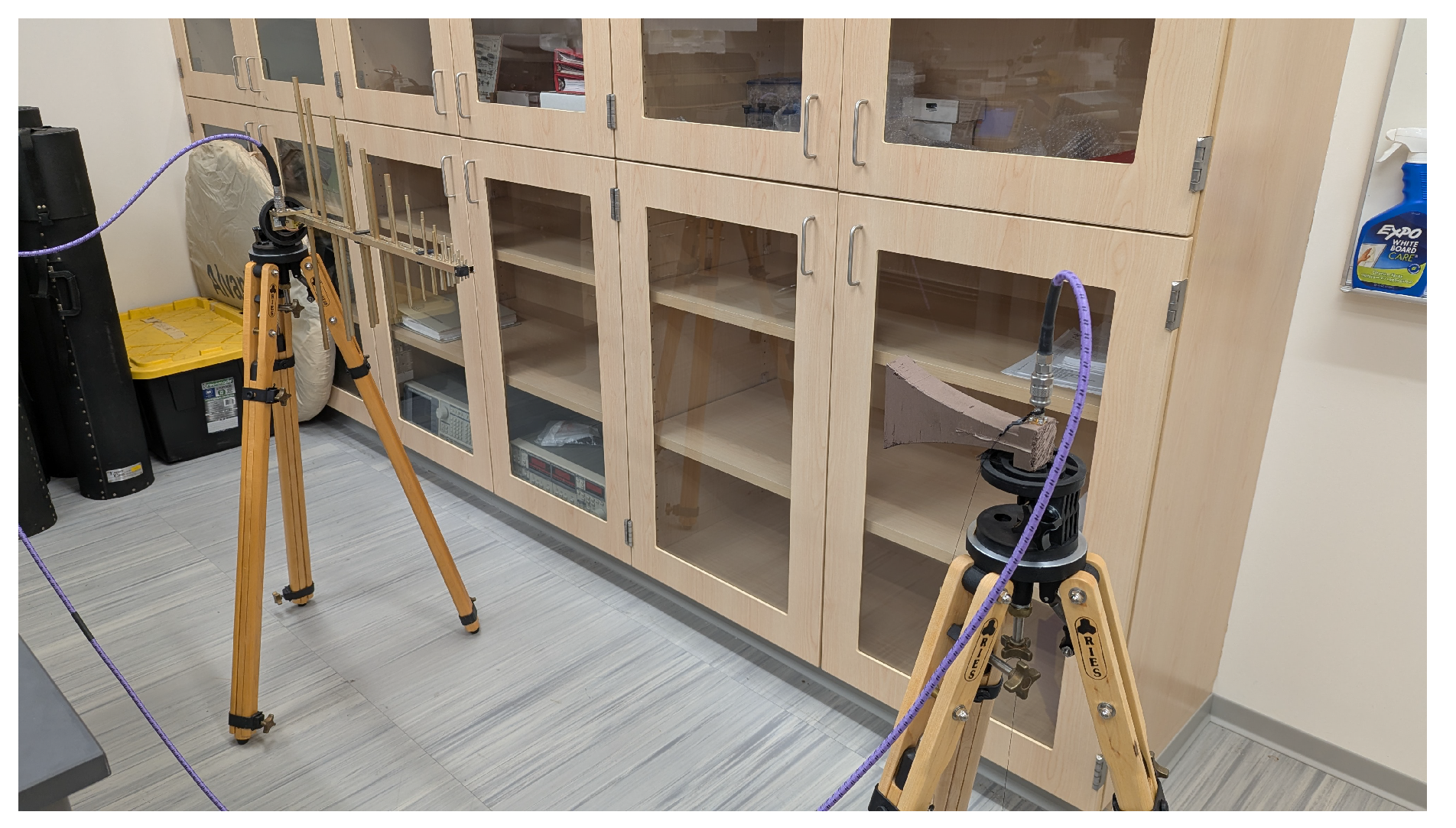
Figure 6.
(Left) Black circles: the -plane radiation pattern data (5.967 GHz). Black line: 3D MEEP simulation of -plane radiation pattern. (Right) Black crosses: the -plane radiation pattern data (5.85 GHz). Black line: 3D MEEP simulation of -plane radiation pattern.
Figure 6.
(Left) Black circles: the -plane radiation pattern data (5.967 GHz). Black line: 3D MEEP simulation of -plane radiation pattern. (Right) Black crosses: the -plane radiation pattern data (5.85 GHz). Black line: 3D MEEP simulation of -plane radiation pattern.
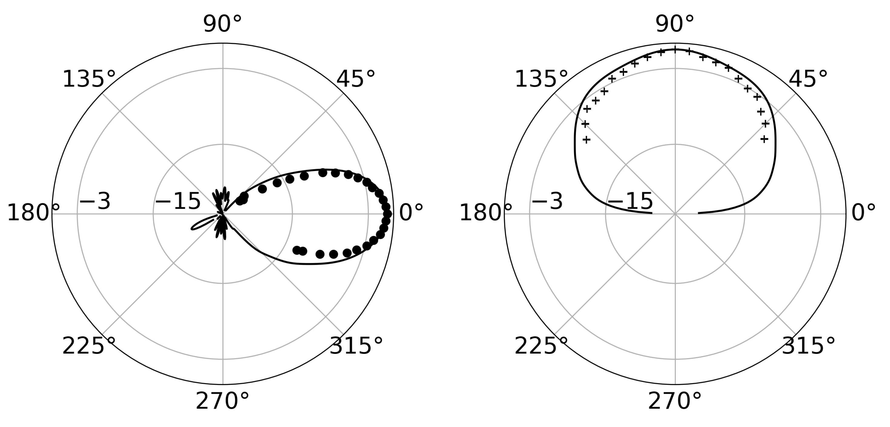
Figure 7.
Circles: measured VSWR data, smoothed with a running average filter. Line: VSWR from MEEP modeling. The black circles have been shifted down to account for the impedance mismatch between 3D printed RF horn and coaxial cable. See text for details.
Figure 7.
Circles: measured VSWR data, smoothed with a running average filter. Line: VSWR from MEEP modeling. The black circles have been shifted down to account for the impedance mismatch between 3D printed RF horn and coaxial cable. See text for details.
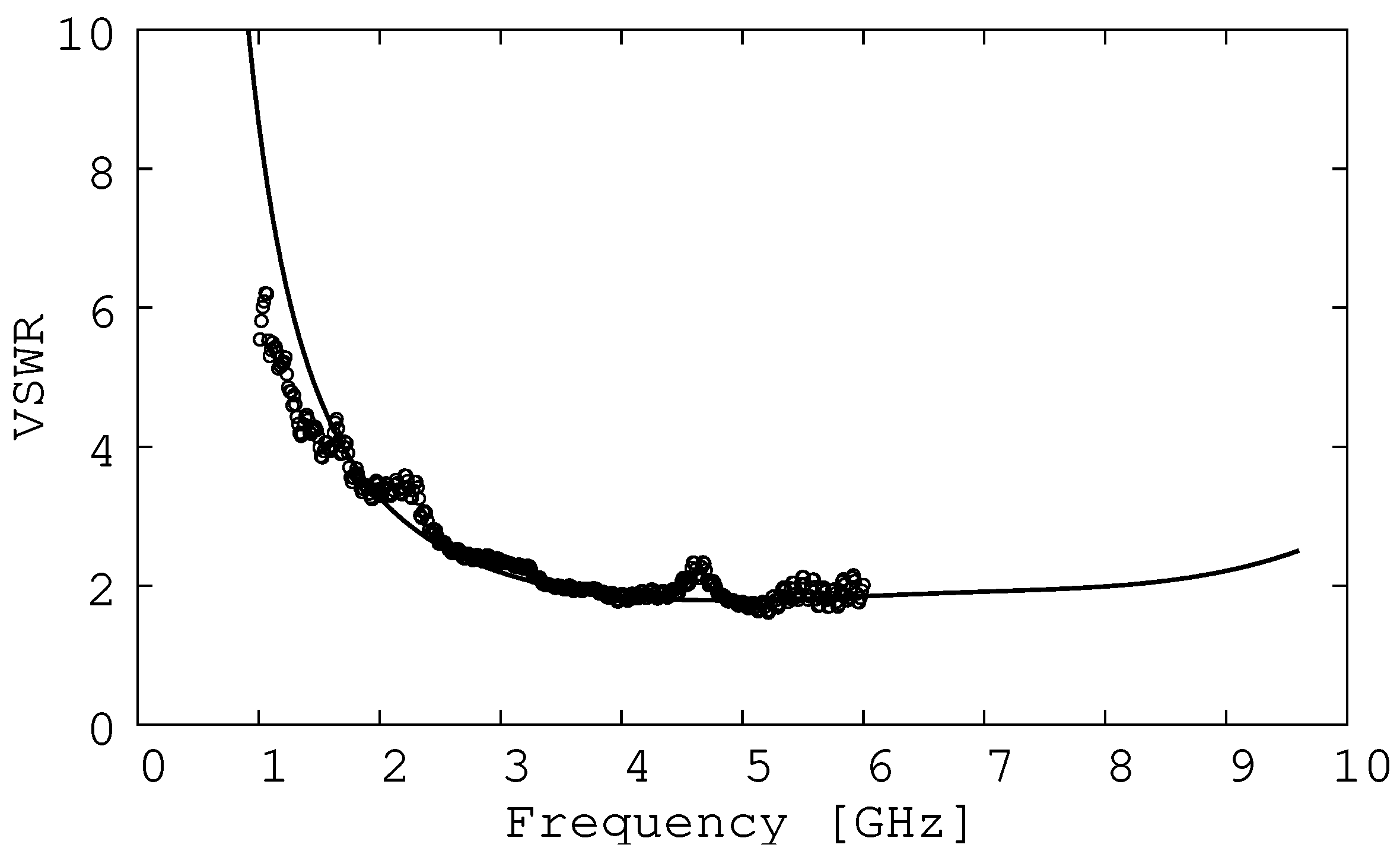
Figure 8.
Circles: measured cross-polarization ratio in dB relative to maximum power. Line: Prediction from Equation 4.
Figure 8.
Circles: measured cross-polarization ratio in dB relative to maximum power. Line: Prediction from Equation 4.
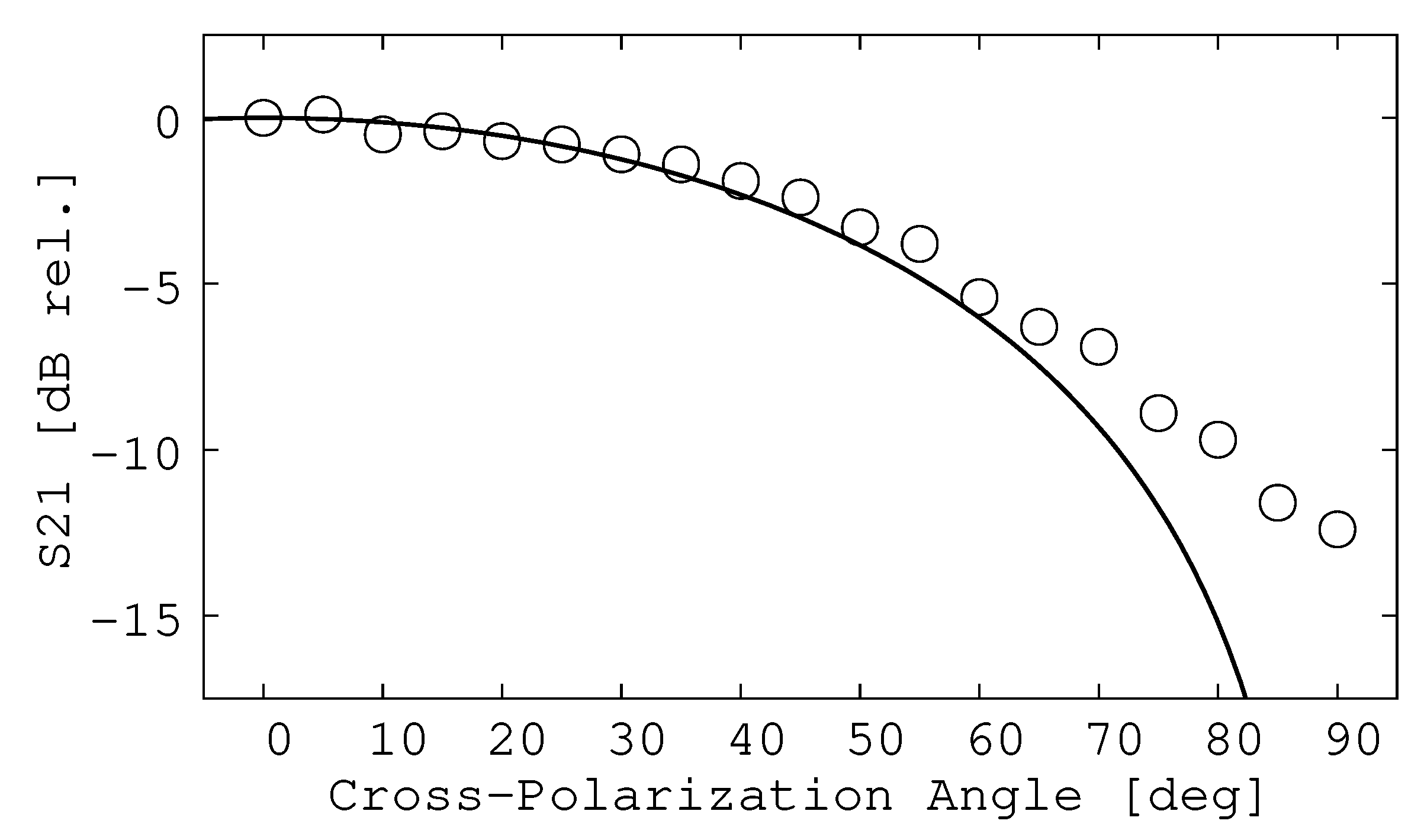
Figure 9.
Black circles: the VSWR data from Figure 7, with frequencies scaled down by a factor of 2. Solid black line: VSWR from MEEP simulation using a CAD model scaled by a factor of 2. Dashed line: the VSWR from MEEP simulation with RF cable and no RF horn.
Figure 9.
Black circles: the VSWR data from Figure 7, with frequencies scaled down by a factor of 2. Solid black line: VSWR from MEEP simulation using a CAD model scaled by a factor of 2. Dashed line: the VSWR from MEEP simulation with RF cable and no RF horn.
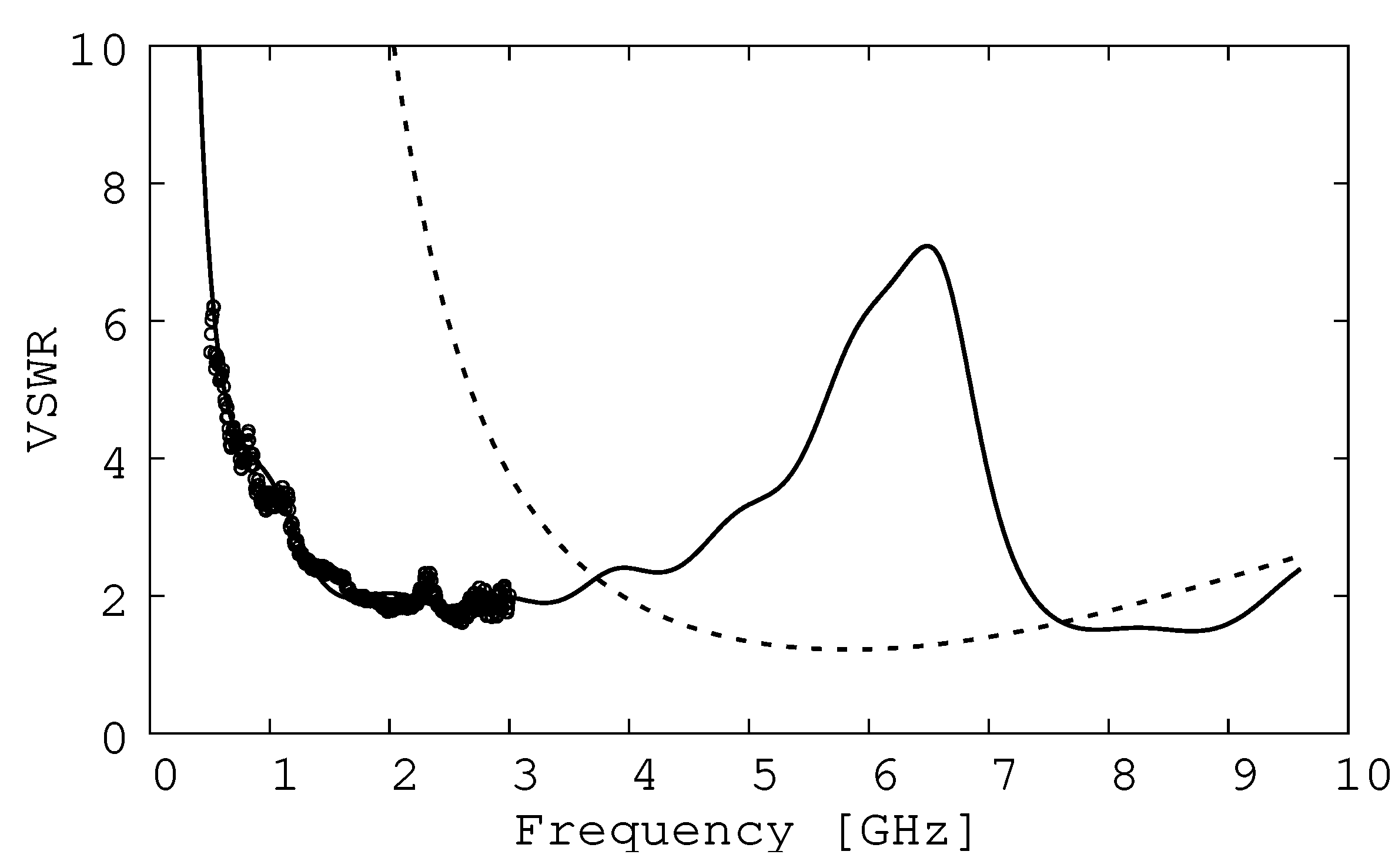

Table 1.
Design parameters for the RF horn antenna.
| Parameter | Variable Name | Value [cm] |
|---|---|---|
| Cavity Length | 0.77 | |
| Cavity Width | 1.00 | |
| Surface Length | 16.52 | |
| Opening Width | w | 9.59 |
| Height | z | 2.0 |
Disclaimer/Publisher’s Note: The statements, opinions and data contained in all publications are solely those of the individual author(s) and contributor(s) and not of MDPI and/or the editor(s). MDPI and/or the editor(s) disclaim responsibility for any injury to people or property resulting from any ideas, methods, instructions or products referred to in the content. |
© 2026 by the authors. Licensee MDPI, Basel, Switzerland. This article is an open access article distributed under the terms and conditions of the Creative Commons Attribution (CC BY) license (http://creativecommons.org/licenses/by/4.0/).
Copyright: This open access article is published under a Creative Commons CC BY 4.0 license, which permit the free download, distribution, and reuse, provided that the author and preprint are cited in any reuse.


