
Submitted:
18 July 2025
Posted:
22 July 2025
You are already at the latest version
Abstract
This paper presents an AI-driven approach to optimize a low-profile, multi-band antenna for direction-finding applications. A Feed-Forward Back Propagation (FFBP) neural network was trained on 84 antenna configurations, simulated using a Method of Moments (MoM)-based tool, to predict resonant frequencies, VSWR, and gain across four frequency bands (433 MHz, 877.5 MHz, 2.4 GHz, and 5.8 GHz). The proposed method dramatically reduces computational cost while maintaining accuracy. Compared to a brute-force approach requiring over 814 full-wave simulations, our technique achieves similar precision with only 84 simulations, followed by 85 rapid AI-based predictions, and a fine-tuning procedure targeting the segments with the highest contribution to the error figure. These results highlight the potential of machine learning to enhance antenna design, particularly for protecting sensitive areas e.g., distributed energy facilities from illegal drone incursions.
Keywords:
multi-band antenna
; artificial intelligence optimization
; machine learning
; neural network
; vehicular applications
; low-profile antenna
; electromagnetic source detection
; direction finding
; backpropagation algorithm
; distributed energy facilities protection
2 Doctoral School of Electronics, Telecommunications and Information Technology, National University of Science and Technology Politehnica of Bucharest, 061071 Bucharest, Romania
1. Introduction
Antenna design must often meet simultaneous and even contradictory constraints, e.g. optimal operation on several frequencies or in a broad frequency band, in terms of directivity, voltage standing wave ratio (VSWR), shape and/or physical size. An initial design can be generated based on physical principles; however, the results can still be different from the target characteristics. Simulation is generally a good choice for performing a fine tuning of the initial structure [1,2,3,4].
In order to avoid structure changes leading to divergent results some authors propose approaches based on evolutionary algorithms [5,6] and machine learning [7,8,9]. It should be noted that such approaches are really needed when physical modeling would be too complex and / or too many configurations have to be simulated.
Mimetic antennas [10,11] are essentially radiating structures that should fit into a given shape and size, as they could not be visually identified. Mobile direction finder equipment [12,13] may use such antennas resembling to a car luggage rack. As an example, triangulation with direction finding mobile equipment using mimetic antennas can be used for protecting energy facilities distributed on large areas from illegal drone incursions [14,15,16].
For multiple band or wideband operation the antenna should provide optimal resonant frequencies, directivity, and gain figures for a given shape and size. Under such constraints the only way to get optimal characteristics is to decide which parts of a fixed shape structure should be made out of a conducting or insulating material [17]. Adjustments may lead to a large number of structures to be simulated and therefore a well-trained machine learning algorithm might help to find the optimal structure much faster than simulating all possible conductor-insulator combinations.
To support the proposed optimization methodology, recent studies have emphasized the importance of prediction volume and model selection in achieving high-accuracy antenna designs. For instance,[18] demonstrates that even a limited number of simulation-based predictions, when strategically chosen, can effectively guide structural antenna optimization using machine learning. Similarly, [19,20,21,22] explore various learning algorithms (ANN, SVM, Random Forest, XGBoost), confirming that both model type and the number of predictions significantly influence the accuracy of VSWR and resonant frequency estimation. For the fine-tuning stage, [23] shows that scaling high-impact structural segments using Bayesian optimization leads to substantial performance gains. Complementarily, [24] illustrates how adjusting slot dimensions via support vector regression enables convergence toward target resonant behavior with minimal error.
In this paper, we propose a two-step procedure to optimize a luggage-rack-like antenna for four frequency bands centered on 433 MHz, 877.5 MHz, 2.4 GHz, and 5.8 GHz. The first step consists of encoding three-segment combinations of conductor and dielectric on each rack bar. We then develop a machine learning algorithm to efficiently choose among all possible configurations the optimal one that minimizes an error figure defined in terms of VSWR and resonant frequencies. The training was performed on a set of configurations chosen by analyzing the potential resonant paths and keeping them fixed. The AI prediction focused on varying the structure of the bars neighboring the potential resonant paths in the least-error configuration of the training set.
The second step of our procedure is a fine-tuning based on scaling the segments with the highest impact on the error figure. The results clearly show that the final antenna structure approaches the target characteristics at an error of less than 5%.
2. Methodology
The antenna should fit the shape of a 1 by 1.3-meter luggage rack with fourteen equally spaced, parallel bars (Figure 1). The gap between the antenna and the car roof acting as a ground should be kept at 10 cm, and the bar diameter at 1.5 cm.
Each bar is considered as made out of three equal length segments; each of them can be either a conductor, or a dielectric rod. We encoded each bar by using a three-bit binary word, where 1 means conductor and 0 dielectric; for a simpler description one can then convert the binary word into a decimal digit between 0 and 7. The most significant bit was considered on the excitation point side.
The first step in designing the initial radiator structure is to ensure that there it will be at least a current path close either to an odd multiple of a quarter wavelength (monopole mode resonance) or a halfwave multiple (patch mode resonance) for each resonant frequency. The configuration providing the closest approximation to a resonant length at each frequency of interest is that with the bars # 3, 5, 6, and 8 providing each of them an open-ended segment i.e., the corresponding code word should be either 4 or 5.
The current paths corresponding to each resonant frequency are shown in Figure 2, and Table 1 shows the resonant path length in terms of wavelength both for monopole mode and patch mode resonance.
A total number of 84 configurations were characterized by using a MoM-based simulator for wire antennas, by applying the resonant path constraint as described before.
A Feed-Forward Back Propagation (FFBP)-type, three-layer neural network algorithm was developed [25,26] and trained with the configurations described before. The input layer consisted of 14 neurons corresponding to the antenna bar encoded as shown above. The output layer had 12 neurons corresponding to the output characteristics i.e., VSWR, resonant frequency, and gain for each of the frequency bands to be covered, and the hidden layer comprised 20 neurons.
In order to assess the overall performance of a given antenna structure we have defined a normalized, multi-objective metric as follows:
where and are the computed resonant frequency for the n-th frequency band, and the corresponding voltage standing wave ratio, respectively; with and were denoted the target (objective) figures. The metric weights equally resonant frequencies and VSWR; it was set such as a VSWR figure below 2 has no effect on the error figure.
It should be emphasized that only configurations with a minimal gain of 2 dBi on each resonant frequency were retained. For each frequency band of operation, the resulting resonant frequency was chosen as corresponding to a minimum of VSWR within the range .
3. Results
The training set was defined as shown in Table 2 and Figure 3 respectively. Configuration #78 in the training set, with the bar sequence [5 6 5 6 5 5 1 5 6 1 6 1 6 1] yields the lowest error figure computed using (1) i.e., ϵ=14.24% along with a gain over 2 dBi on all resonant frequencies and was therefore chosen as a reference for assessing further improvement after applying the ML-based optimization.
After training the neural network, the resulting weights between the neuron layers were stored and used to predict the performance of different antenna structures in terms of resonant frequencies, VSWR, and gain over all the four frequency bands of interest.
For prediction, we analyzed three strategies for choosing the bars on which we scan all possible combinations of conductor and dielectric segments. First, we choose to scan all the combinations for the bars neighboring those corresponding to the resonant paths i.e., #2, 4, 7, and 9. The rationale behind this choice was based on the fact that the neighboring bars would mostly affect the resonance through mutual coupling. That is, the prediction was performed on a total number of 84 = 4,096 configurations. After excluding the structures providing a gain below 2dBi the resulting optimal configuration is [5 2 5 0 5 5 4 5 3 1 6 1 6 1] (Figure 4a). The resulting error figure for the optimal configuration is ϵ=13.47%.
Next, we also scanned all the conductor/dielectric combinations on bar #1; the first bar includes the feed point, and therefore the stub configuration may impact on the input impedance. We analyzed 85 = 32,768 configurations; by running the prediction algorithm, a minimum of the error figure i.e., ϵ=13.078% was found for the combination [5 0 5 0 5 5 4 5 7 1 6 1 6 6] (Figure 4b).
We further include in the scanning process the last bar i.e., #14. Thus, the prediction was performed on a total number of 86 = 262,144 configurations. The resulting optimal configuration is [4 0 5 0 5 5 4 5 7 1 6 1 6 7] (Figure 4c) yields an error figure ϵ=13.077%. It comes out that the last bar does not essentially impact on the error figure; conversely, the computing effort was multiplied by 8, compared to the second scanning strategy.
The optimal configuration was then simulated by using the same MoM simulator as for the training set, and the results were compared to those predicted by the ML algorithm (Table 3).
Figure 5, Figure 6, Figure 7and Figure 8 illustrate the VSWR variation for each frequency band considered, as well as the corresponding radiation patterns at the resonant frequency in the E-plane and H-plane.
In order to further optimize the antenna performances and ensure resonance at the target frequencies, a detailed analysis of the current distribution along each segment was conducted. The study revealed that the feed segment plays a predominant role in achieving a resonance at 2.4 GHz, whereas segment 1 of bar #1 has the most significant influence on the resonance at 433 MHz. Consequently, a fine-tuning approach based on segment scaling was applied, as follows:
the feed segment was lengthened from 5 cm to 6.25 cm to shift the resonance closer to 2.4 GHz;
segment 1 of bar #1 was extended from 33 cm to 38 cm to provide resonance at 433 MHz.
Figure 9 illustrates the antenna structure after the fine-tunning.
Figure 10 illustrates the VSWR variation for each frequency band for the optimized antenna structure. Table 4 shows the characteristics of the final antenna design. Figure 11, Figure 12 and Figure 13 show the radiation patterns corresponding to the resonance frequency in the E-plane and H-plane.
After performing the fine tuning as shown before the error figure as defined in (1) went down to 3.41%.
4. Conclusions
This work presents a method to generate a multi-band antenna, based on a fixed-shape structure imitating a car luggage-rack.
The first step was to encode each bar of the structure as a three-bit code word, and to apply an artificial intelligence approach to minimize an error figure targeting a VSWR less than 2 and to minimize the discrepancies between the resonant frequencies and the frequencies of interest.
The results demonstrate the effectiveness of the machine learning-based optimization in identifying an improved antenna configuration, with the error figure reduced from 14.24% to 13.078%. This improvement suggests that the best-performing configuration from the training set was already close to the optimal solution.
Moreover, the computational efficiency gain is substantial. While a brute-force approach would require 814 = 4,398,046,511,104 full-wave simulations, our method achieved comparable accuracy using only 84 simulations for training, followed by 85=32,768 rapid predictions. This represents a dramatic reduction in computational cost while maintaining precision, proving the capability of AI-driven techniques to accelerate and enhance antenna design optimization. We show that a higher number of predictions e.g., 86 = 262,144 configurations improves the error figure by only 0.001 % at a computing time eight times longer. We can therefore conclude that an error-to-computing time tradeoff has been reached for our three-bit bar encoding scheme.
The next step was to further reduce the error figure by scaling the segment dimensions to fine-tune the resonant frequencies, allowing for better control of the antenna multi-band operation. Size scaling targeted the segments virtually leading the higher shift in resonant frequency and thus, the final error figure was made as low as 3.41%.
Further enhancements can be achieved by refining both the antenna design parameters and the neural network model. Additionally, increasing the number of segments per bar would provide a finer mesh in the optimization process, potentially leading to superior configurations. Yet, increasing the number of segments leads to a larger number of configurations and might therefore increase the computing time more than size scaling on targeted segments would do.
From a machine learning perspective, several factors could be explored to enhance prediction accuracy. These include adjusting the number of neurons in the hidden layer, increasing the number of hidden layers, and evaluating alternative neural network architectures and training algorithms.
By integrating these refinements, the proposed approach can achieve even greater accuracy and efficiency, further advancing AI-driven antenna design methodologies.
Author Contributions
Conceptualization, R.D.T.; methodology, R.D.T.; software, R.D.T.; validation, R.D.T.; formal analysis, R.D.T.; investigation, R.D.T.; resources, R.D.T.; data curation, R.D.T.; writing—original draft preparation, R.D.T.; writing—review and editing, R.D.T.; visualization, R.D.T.; supervision, R.D.T.; project administration, R.D.T.; funding acquisition, R.D.T. All authors have read and agreed to the published version of the manuscript.
Data Availability Statement
Ongoing research project requiring confidential data status.
Acknowledgments
This work was supported under the project MAREHC, a grant of the Romanian Ministry of Research, Innovation and Digitalization, project number PNRR-C9-I8-760111/23.05.2023, code CF 48/14.11.2022, within PNRR. .
Conflicts of Interest
The authors declare no conflicts of interest.
Abbreviations
The following abbreviations are used in this manuscript:
| ANN | Artificial Neural Network |
| FFBP | Feed-Forward Back Propagation |
| ML | Machine Learning |
| MOM | Method of Moments |
| VSWR | Voltage Standing Wave Ratio |
References
- J. Khan and G. Kiani, “Parametric study of microstrip patch antenna on LCP substrate for 70 GHz applications,” in 2015 IEEE 4th Asia-Pacific Conference on Antennas and Propagation (APCAP), Jun. 2015, pp. 554–555. [CrossRef]
- F. Shariar and Md. F. Hossain, “Design and Analysis of a Triple Band Microstrip Patch Antenna for Wireless Applications,” in 2023 6th International Conference on Electrical Information and Communication Technology (EICT), Dec. 2023, pp. 1–6. [CrossRef]
- Constantin, G. Ifrim, and R. D. Tamas, “Innovative Dual-Band Antenna for Reliable LoRa IoT Connectivity,” in 2024 Advanced Topics on Measurement and Simulation (ATOMS), Aug. 2024, pp. 81–84. [CrossRef]
- C.-A. Heiman, A. C.-A. Heiman, A. Constantin, M. Pastorcici, and R. D. Tamas, “Wideband Circularly Polarized FSS-Horn Antennas,” in 2023 IEEE-APS Topical Conference on Antennas and Propagation in Wireless Communications (APWC), Oct. 2023, pp. 035–037. [CrossRef]
- J. Liu, Y. J. Liu, Y. Yang, N. Li, and K. Xie, “Optimization of Broadband Patch Antenna Based on Mind Evolutionary Algorithm,” in 2009 International Conference on Networks Security, Wireless Communications and Trusted Computing, Apr. 2009, pp. 361–364. [CrossRef]
- S. Bucuci et al., “A Compact Monopole Antenna for Underwater Acoustic Monitoring Beacons,” Sensors, vol. 22, no. 21, Art. no. 21, Jan. 2022. [CrossRef]
- N. Aulia Yusuf, P. D. N. Aulia Yusuf, P. D. Purnamasari, and F. Y. Zulkifli, “A Comparative Analysis of Machine Learning Algorithms for Predicting the Dimensions of Rectangular Microstrip Antennas,” in 2023 IEEE International Symposium On Antennas And Propagation (ISAP), Oct. 2023, pp. 1–2. [CrossRef]
- Gampala and C., J. Reddy, “Fast and Intelligent Antenna Design Optimization using Machine Learning,” in 2020 International Applied Computational Electromagnetics Society Symposium (ACES), Jul. 2020, pp. 1–2. [CrossRef]
- M. E. Misilmani and T. Naous, “Machine Learning in Antenna Design: An Overview on Machine Learning Concept and Algorithms,” in 2019 International Conference on High Performance Computing & Simulation (HPCS), Jul. 2019, pp. 600–607. [CrossRef]
- Alieldin, *!!! REPLACE !!!*; et al. , “A Camouflage Antenna Array Integrated with a Street Lamp for 5G Picocell Base Stations,” in 2019 13th European Conference on Antennas and Propagation (EuCAP), Mar. 2019, pp. 1–4. Accessed: Mar. 12, 2025. [Online]. Available: https://ieeexplore.ieee. 8739. [Google Scholar]
- Sanz-Izquierdo, F. Huang, and J. C. Batchelor, “Small size wearable button antenna,” in 2006 First European Conference on Antennas and Propagation, Nov. 2006, pp. 1–4. [CrossRef]
- “Radio Direction Finder (RDF),” Doppler Systems, LLC. Accessed: Mar. 17, 2025. [Online]. Available: https://dopsys.
- K. N. J. Purwanto, A. K. N. J. Purwanto, A. Yahya, N. H. H. Khamis, N. M. Nor, M. R. Shaari, and A. R. M. Sidek, “Development of Radio Direction Finder using 6 Log Periodic Dipole Array Antennas,” in 2018 5th International Conference on Information Technology, Computer, and Electrical Engineering (ICITACEE), Sep. 2018, pp. 157–160. [CrossRef]
- F.-L. Chiper, A. F.-L. Chiper, A. Martian, C. Vladeanu, I. Marghescu, R. Craciunescu, and O. Fratu, “Drone Detection and Defense Systems: Survey and a Software-Defined Radio-Based Solution,” Sensors, vol. 22, no. 4, Art. no. 4, Jan. 2022. [Google Scholar] [CrossRef]
- Famili, A. Stavrou, H. Wang, J.-M. (Jerry) Park, and R. Gerdes, “Securing Your Airspace: Detection of Drones Trespassing Protected Areas,” Sensors, vol. 24, no. 7, Art. no. 7, Jan. 2024. [Google Scholar] [CrossRef]
- Łukasiewicz and, A. Kobaszyńska-Twardowska, “Proposed method for building an anti-drone system for the protection of facilities important for state security,” Security and Defence Quarterly, Jun. 2022. [Google Scholar] [CrossRef]
- Heiman and R., D. Tamas, “Transforming Linear to Circular Polarization on Horn Antennas by Using Multiple-Layer Frequency Selective Surfaces,” Sensors, vol. 22, no. 20, Art. no. 20, Jan. 2022. [Google Scholar] [CrossRef]
- Bazgir, A. Sheikhi, and M. Dowlatshahi, “Resonance frequency prediction of dielectric antennas for liquid sensing via support vector regression,” Scientific Reports, vol. 14, Dec. 2024. [Google Scholar] [CrossRef]
- O. Singh, M. O. Singh, M. Bharamagoudra, H. Gupta, A. Dwivedi, P. RANJAN, and A. Sharma, “Microstrip line fed dielectric resonator antenna optimization using machine learning algorithms,” Sādhanā, vol. 47, Nov. 2022. [Google Scholar] [CrossRef]
- Heiman and R., D. Tamas, “Neural Network-Based Predictive Design of FSS Structures for Satellite Antenna Performance Enhancement,” IEEE International Conference on Antenna Measurements and Applications (CAMA)-Special Sessions: SPS16 New Technologies and Methodologies for Antenna Design, Antibes, France, Nov. 2025 (in press).
- Constantin and R., D. Tamas, “A Multi-Band AI-Miniaturized Patch Antenna for Environmental Monitoring,”IEEE International Conference on Antenna Measurements and Applications (CAMA)-Special Sessions: SPS16 New Technologies and Methodologies for Antenna Design, Antibes, France, Nov. 2025 (in press).
- RANJAN, H. Gupta, A. Sharma, S. Yadav, and M. Potrebićc, “Investigation and Optimization of Dielectric Resonator MIMO Antenna Using Machine Learning Approach,” 2022, pp. 645–655. [CrossRef]
- C.-H. Huang, A. C.-H. Huang, A. Ali, C.-C. Hsu, and H.-H. Tsao, Enhanced Antenna Design through Hyper parameter Optimization of Diverse Machine Learning Models Using Bayesian Optimization. 2024. [CrossRef]
- T. Khan and C. Roy, “Prediction of slot-position and slot-size of a microstrip antenna using support vector regression,” International Journal of RF and Microwave Computer-Aided Engineering, vol. 29, Dec. 2018. [CrossRef]
- O. A. Abdalla, M. N. O. A. Abdalla, M. N. Zakaria, S. Sulaiman, and W. F. W. Ahmad, “A comparison of feed-forward back-propagation and radial basis artificial neural networks: A Monte Carlo study,” in 2010 International Symposium on Information Technology, Jun. 2010, pp. 994–998. [CrossRef]
- E. Stamos, estamos/Neural-Network-Design-Solutions-Manual. (Feb. 20, 2025). R. Accessed: Mar. 14, 2025. [Online]. Available: https://github.
Figure 1.
Antenna shape.
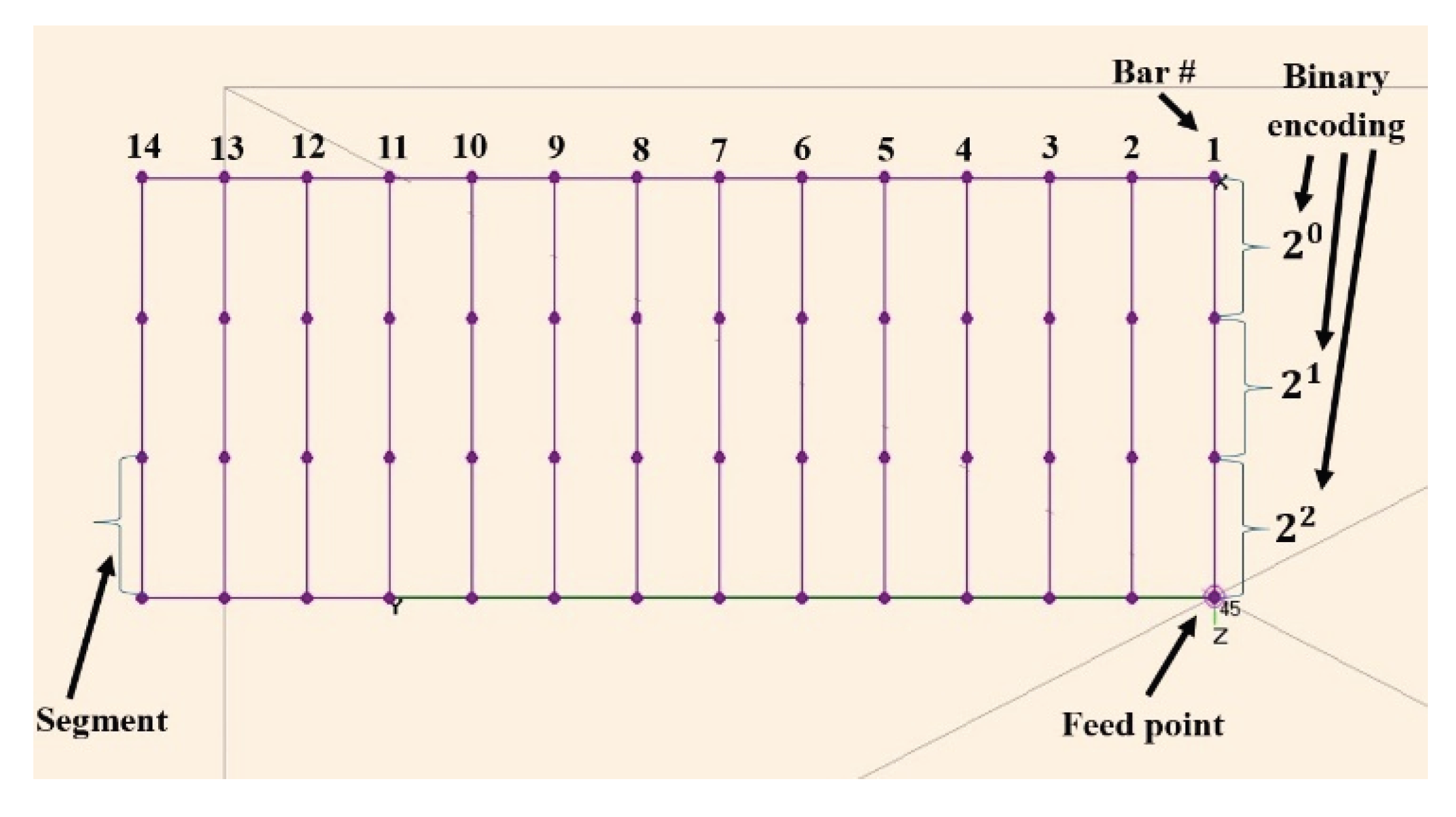
Figure 2.
Possible resonant current paths.
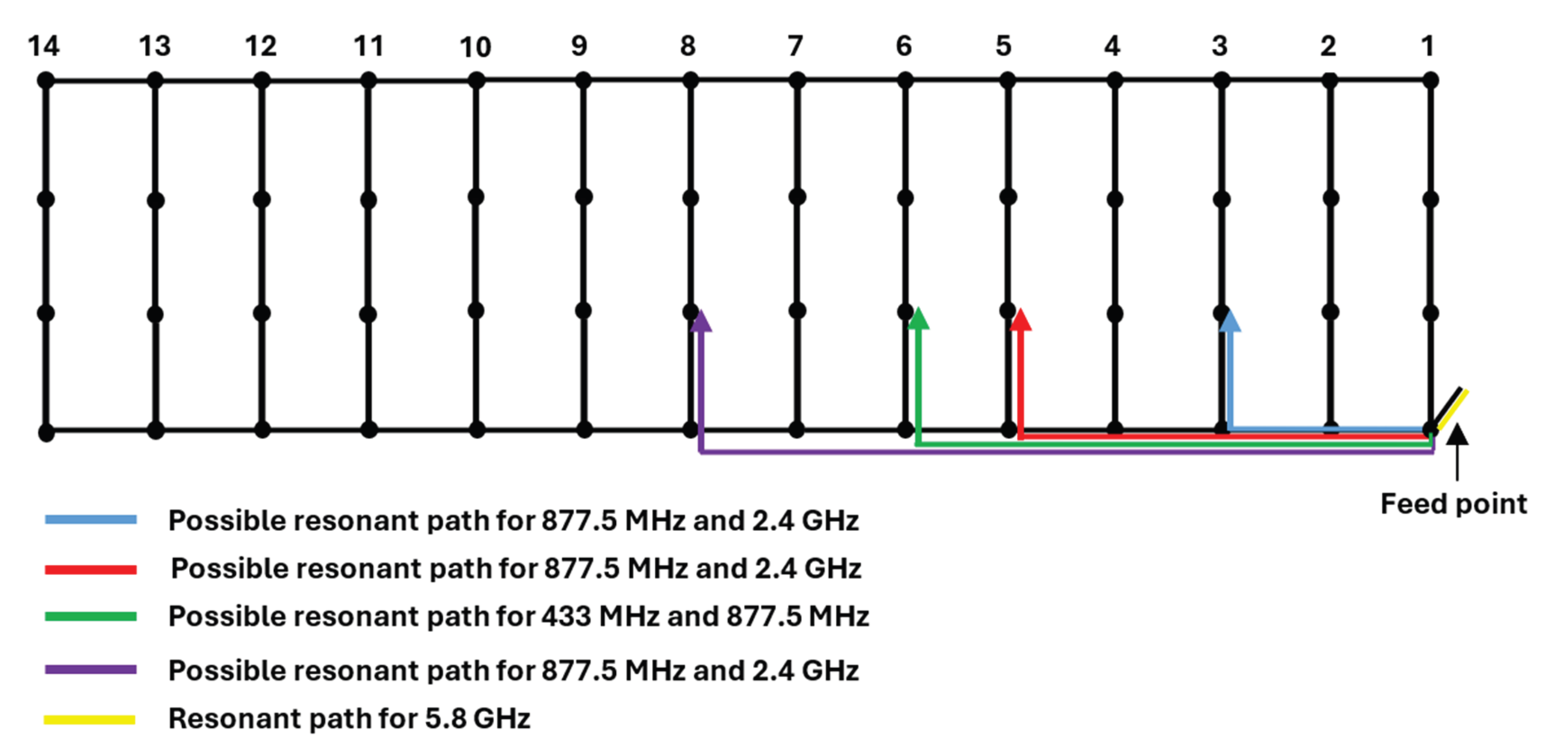
Figure 3.
(a) Configuration #1 – 42; (b) Configuration #43 – 63; (c) Configuration #64 – 84.
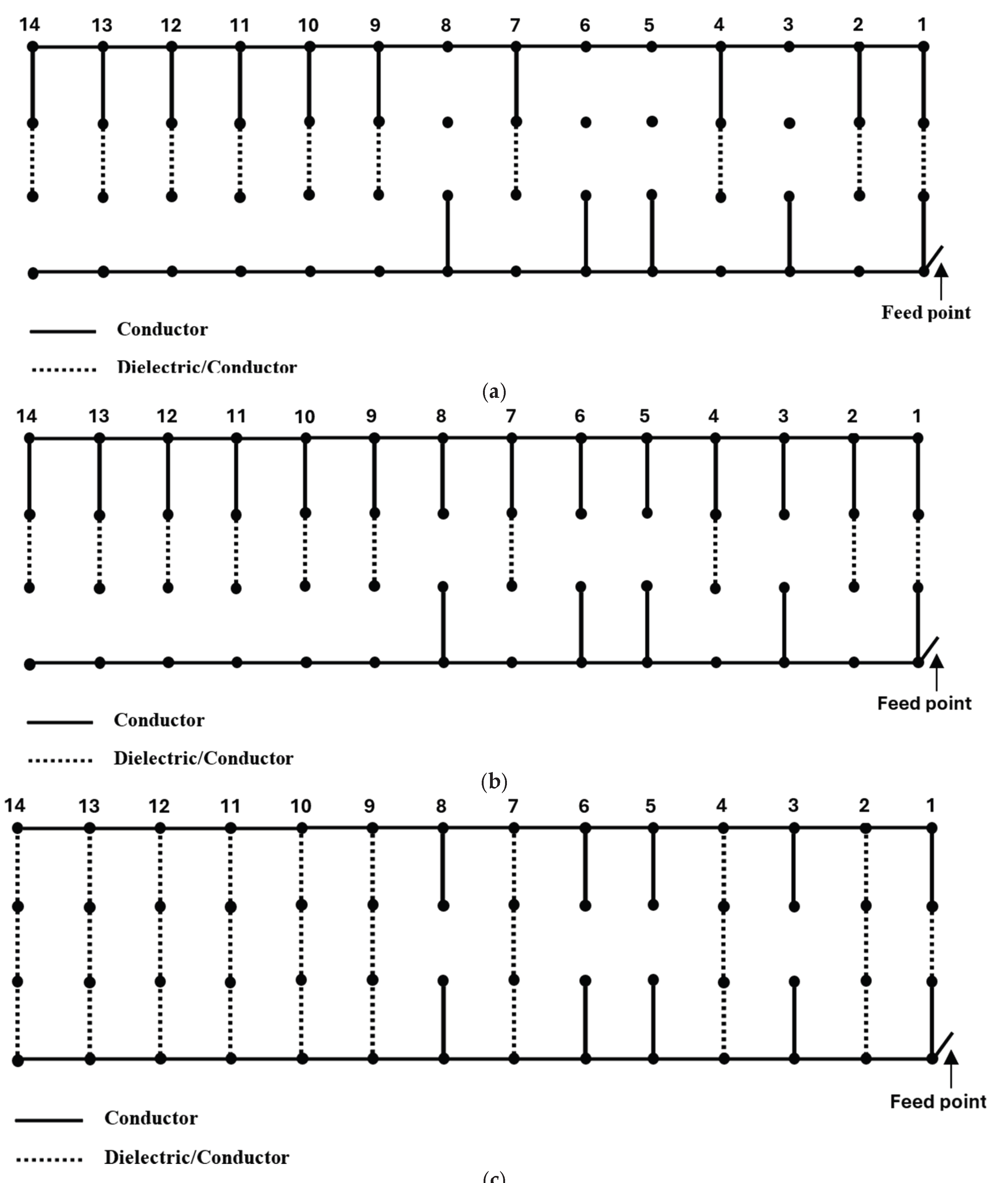
Figure 4.
Optimal configuration predicted by the ML algorithm for different strategies on scanning the combinations of conductor and dielectric segments: (a) bars neighboring the resonant paths; (b) first bar and bars neighboring the resonant paths; (c) first bar, last bar, and bars neighboring the resonant paths.
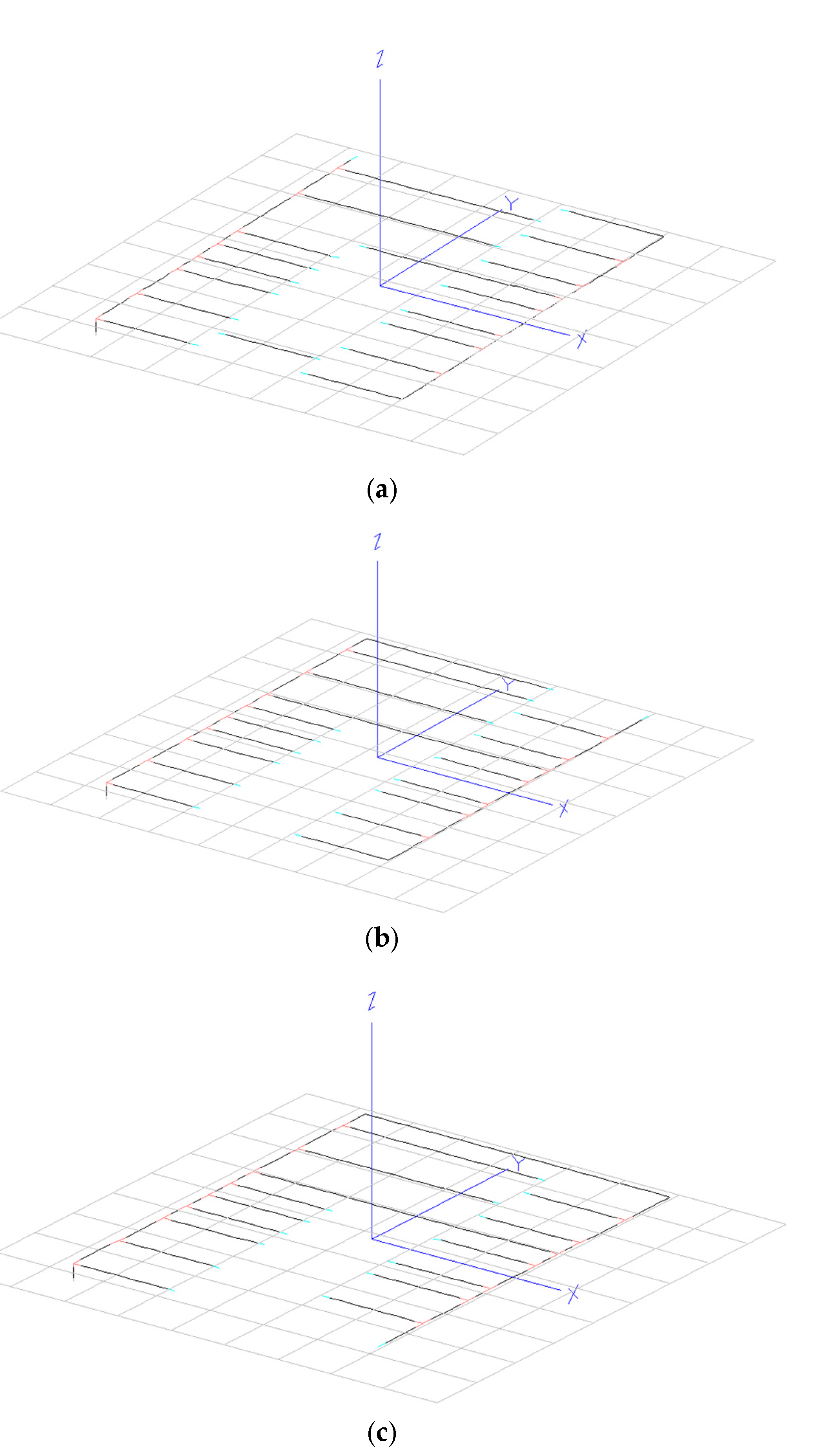
Figure 5.
VSWR variation for: (a) 433 MHz; (b) 877 MHz; (c) 2.4 GHz; (d) 5.8 GHz bands.
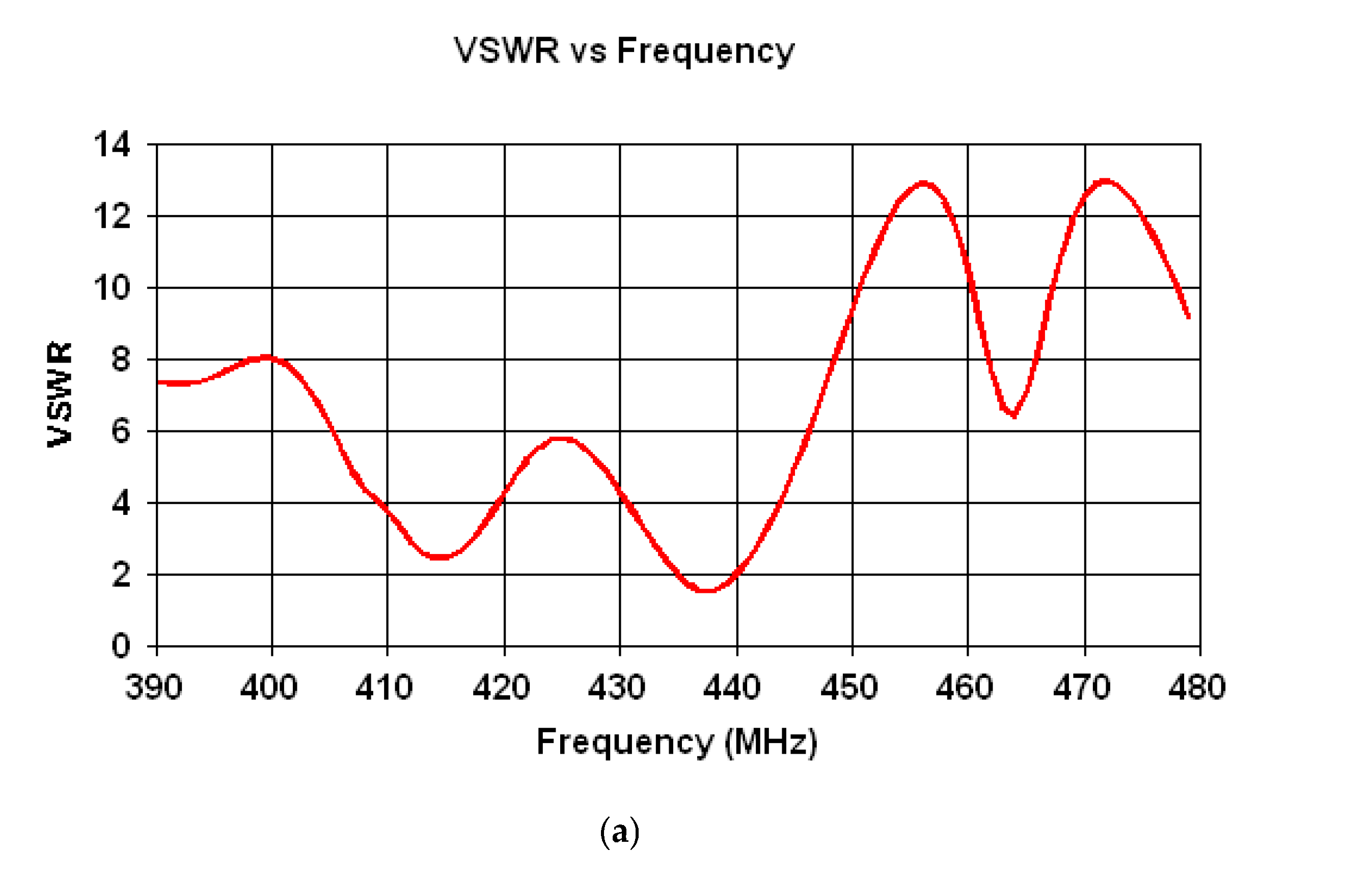
Figure 6.
Gain in the H-plane: (a) 433 MHz, θ=26°; (b) 877 MHz, θ=-42°; (c) 2.4 GHz, θ=53°; (d) 5.8 GHz, θ=-45°.
Figure 6.
Gain in the H-plane: (a) 433 MHz, θ=26°; (b) 877 MHz, θ=-42°; (c) 2.4 GHz, θ=53°; (d) 5.8 GHz, θ=-45°.
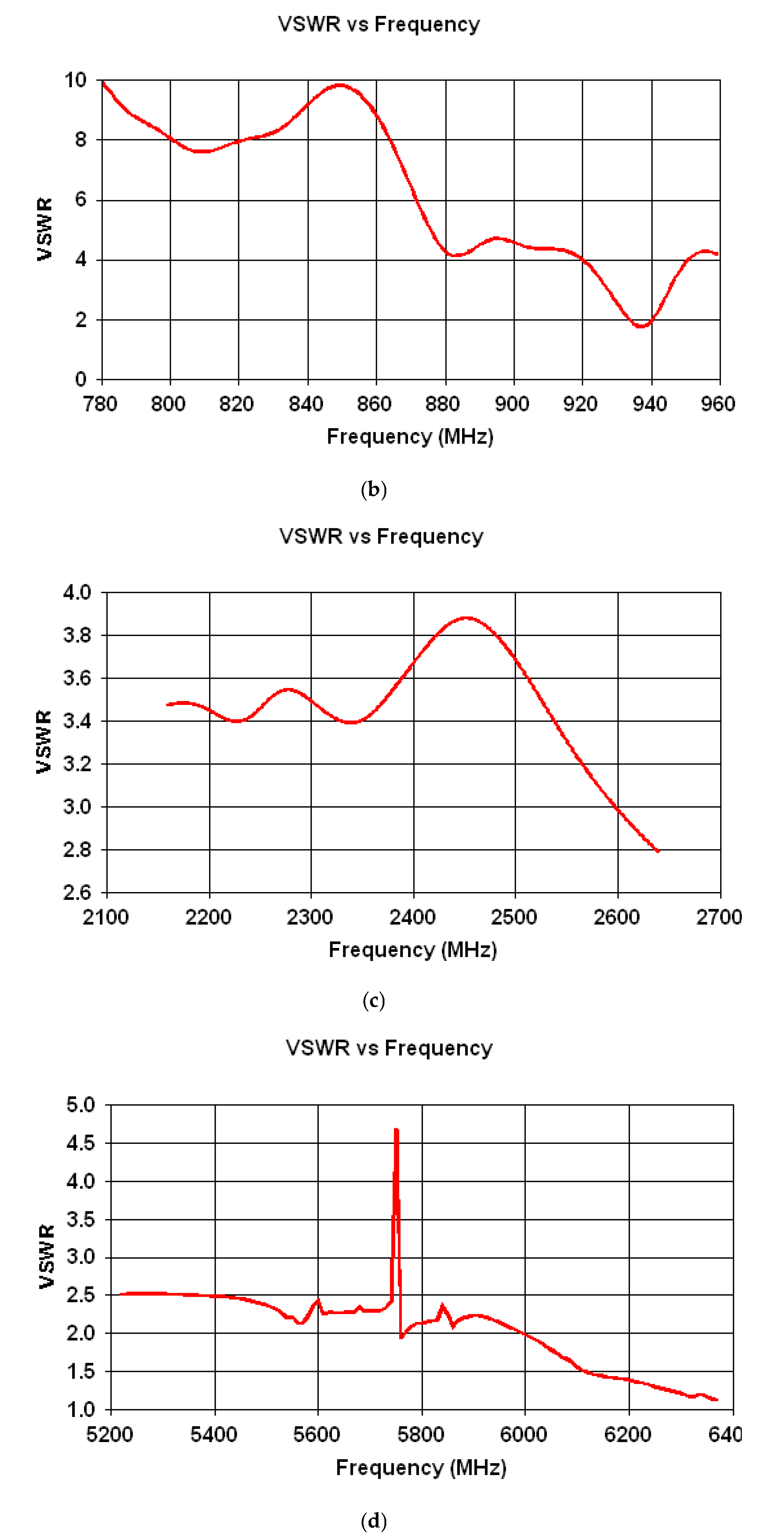
Figure 7.
Gain in the E-plane for : (a) 433 MHz; (b) 877 MHz; (c) 2.4 GHz; (d) 5.8 GHz.
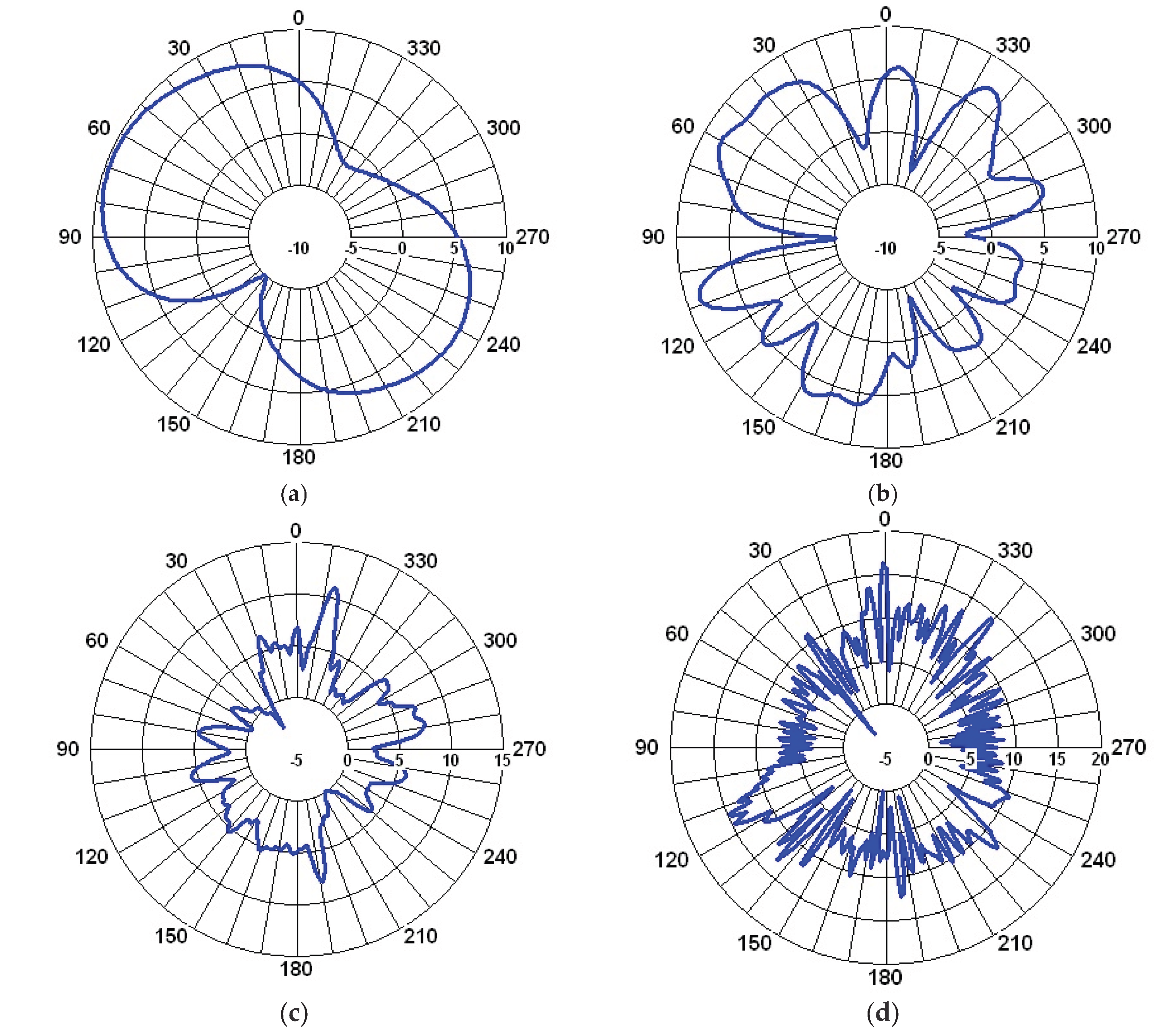
Figure 8.
Gain in the E-plane for : (a) 433 MHz; (b) 877 MHz; (c) 2.4 GHz; (d) 5.8 GHz.
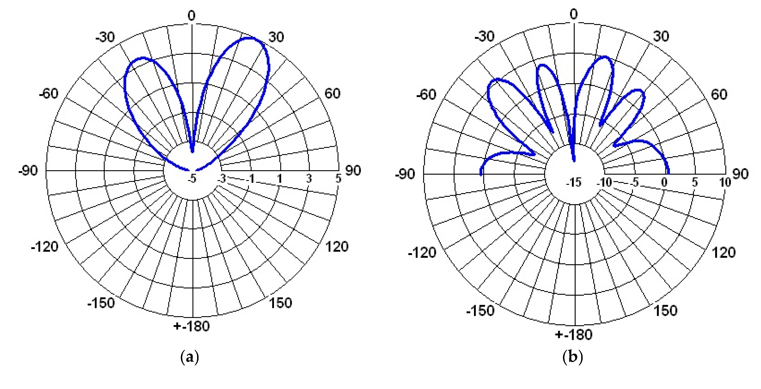
Figure 9.
Antenna structure after the fine-tunning.
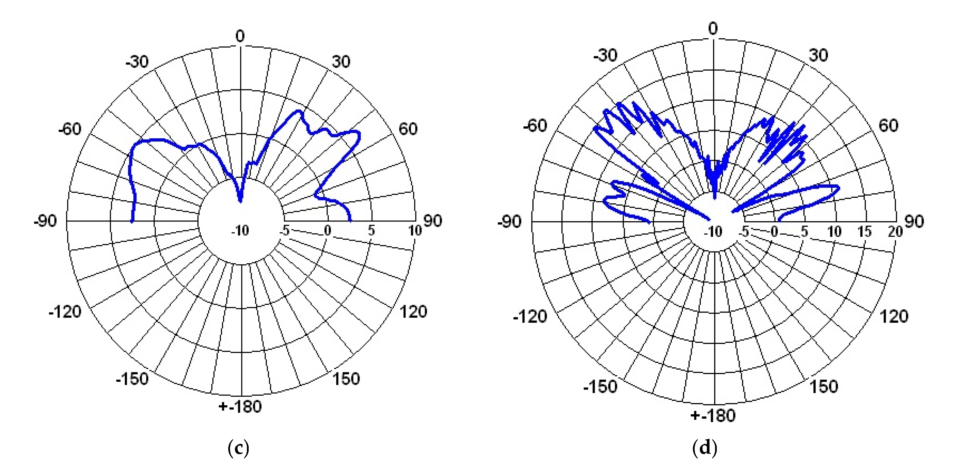
Figure 10.
VSWR variation for (a) 433 MHz; (b) 877 MHz; (c) 2.4 GHz; (d) 5.8 GHz bands.
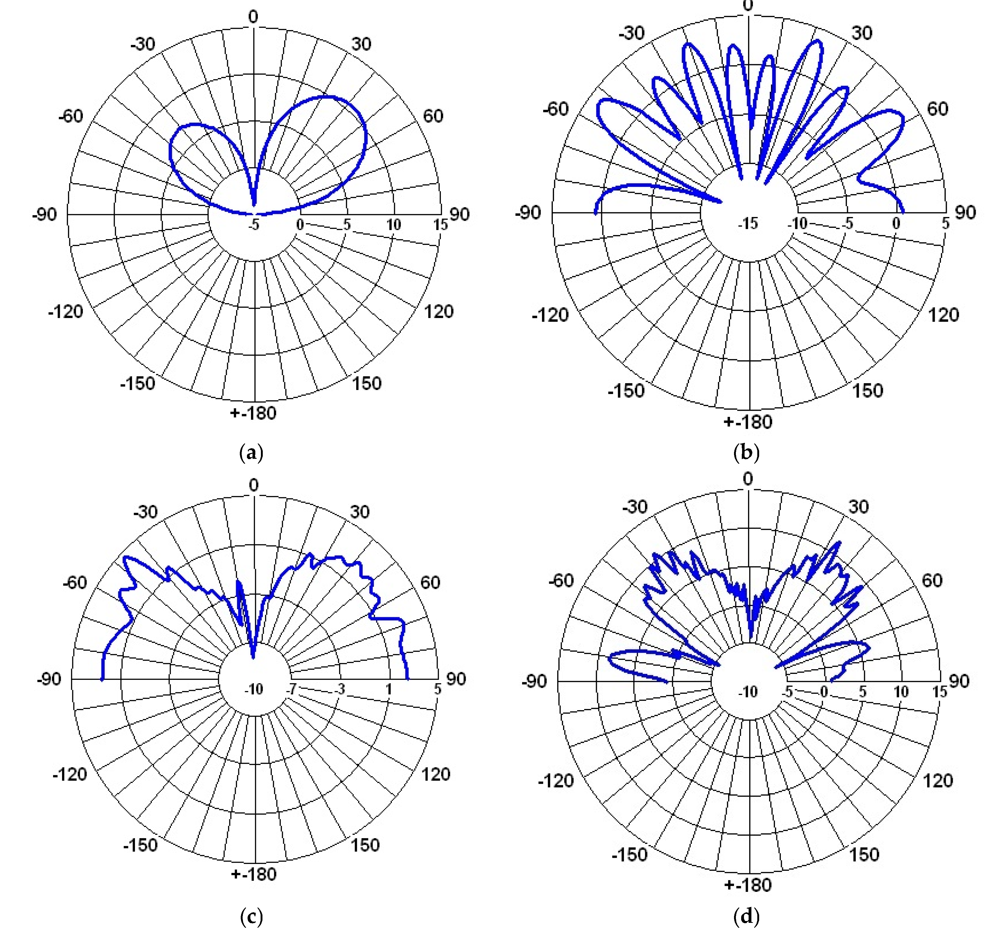
Figure 11.
Gain in the H-plane: (a) 433 MHz, θ=26°; (b) 877 MHz, θ=41°; (c) 2.4 GHz, θ=50°; (d) 5.8 GHz, θ=52°.
Figure 11.
Gain in the H-plane: (a) 433 MHz, θ=26°; (b) 877 MHz, θ=41°; (c) 2.4 GHz, θ=50°; (d) 5.8 GHz, θ=52°.
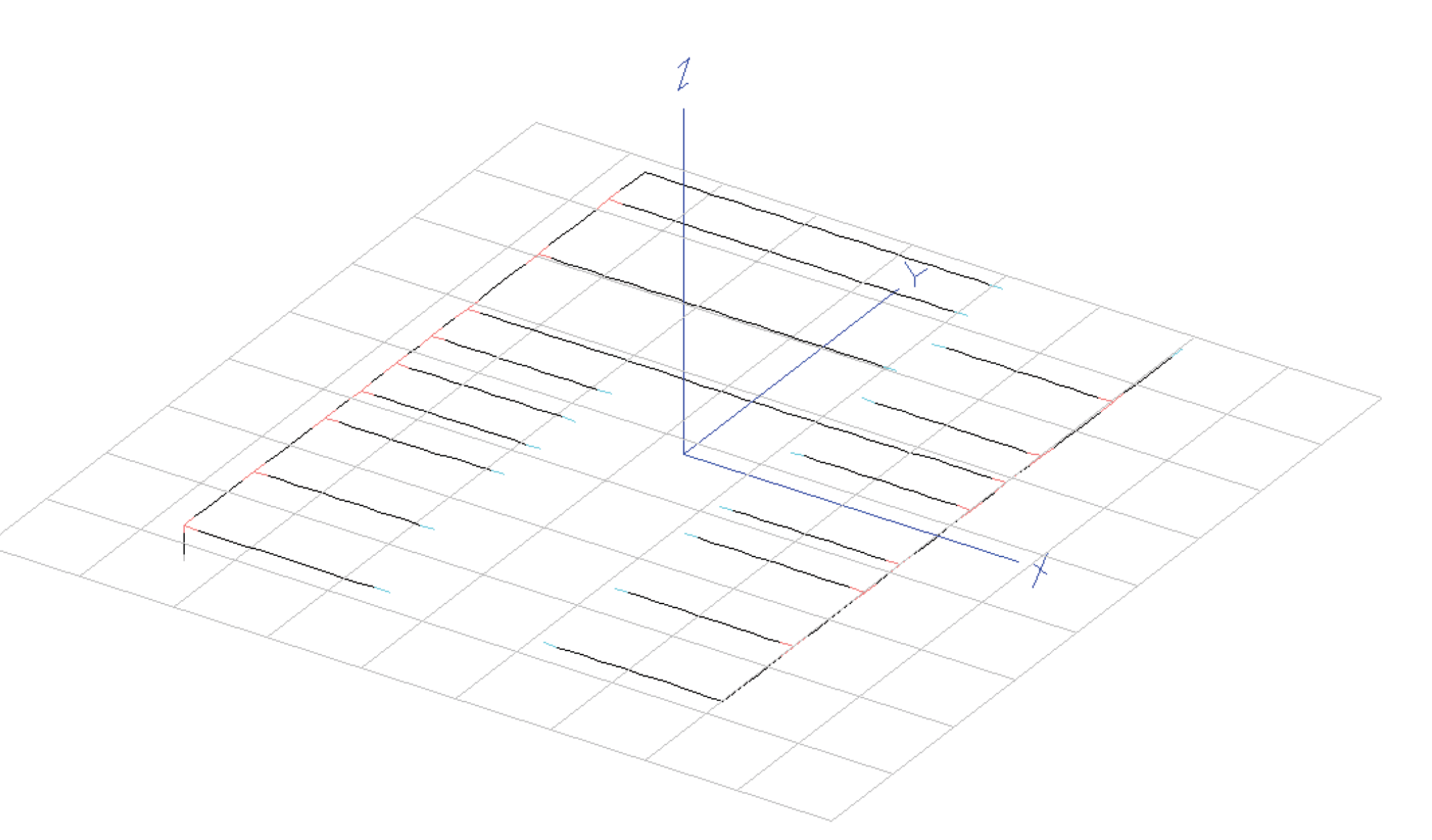
Figure 12.
Gain in the E-plane for : (a) 433 MHz; (b) 877 MHz; (c) 2.4 GHz; (d) 5.8 GHz.
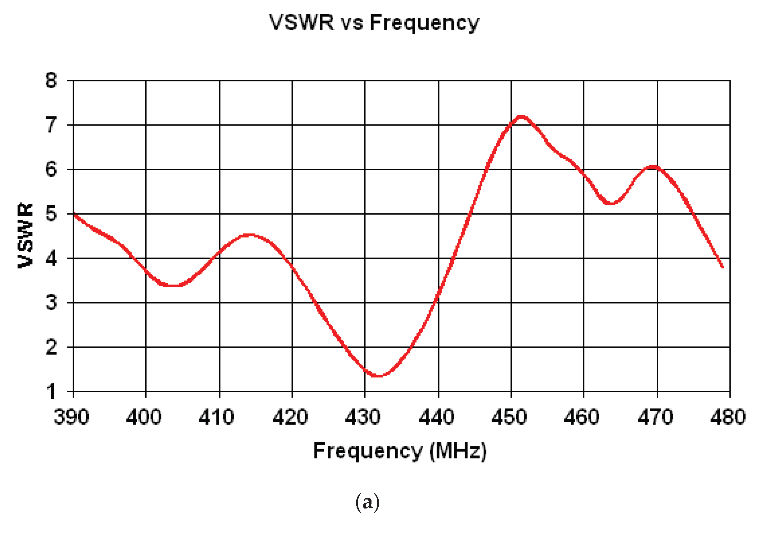
Figure 13.
Gain in the E-plane for : (a) 433 MHz; (b) 877 MHz; (c) 2.4 GHz; (d) 5.8 GHz.


Table 1.
Possible resonant path length in terms of wavelength: patch mode resonance and monopole mode resonance.
Table 1.
Possible resonant path length in terms of wavelength: patch mode resonance and monopole mode resonance.
| Resonant Path | Patch Mode Resonance (Multiple of λ/2) | Monopole Mode Resonance (Odd Multiple of λ/4) | |
|---|---|---|---|
| Color (ref. Figure 2) | Length [m] | ||
| Blue | 0.58 | 5 λ at 2.4 GHz | aprox. 1.75 λ at 877 MHz |
| Red | 0.78 | 6.5 λ at 2.4 GHz | aprox. 2.25 λ at 877 MHz |
| Green | 0.88 | 2.5 λ at 877.5 MHz | aprox. 1.25 λ at 433 MHz |
| Purple | 1.08 | 9 λ at 2.4 GHz 1.5 λ at 433 MHz |
aprox. 3.25 λ at 877 MHz |
| Yellow | 0.05 | aprox λ/2 at 2.4 GHz | aprox. λ at 5.8 GHz |
Table 2.
Training set.
| Configuration | Code Word for the Resonant Bars (#3, 5, 6, and 8) | Code Word for the Bars #1, 2, 4, 7, and 9 - 14 |
|---|---|---|
| #1 - 42 | 4 | 5 or 7 for #1; 1 or 3 for the rest |
| #43 - 63 | 5 | 5 or 7 for #1; 1 or 3 for the rest |
| #64 - 84 | 5 | 5 or 7 for #1; 1 or 6 for the rest |
Table 3.
Optimal configuration: prediction versus simulation.
| Frequency Band [MHz] | Resonant Frequency – Prediction [MHz] |
Resonant Frequency – Simulation [MHz] |
VSWR – Prediction |
VSWR – Simulation |
Gain – Simulation [dBi] |
Gain – Simulation [dBi] |
|---|---|---|---|---|---|---|
| 433 | 433 | 438 | 1.97 | 1.5 | 4.31 | 5 |
| 877.5 | 894 | 937 | 2.06 | 1.75 | 7.33 | 5.65 |
| 2400 | 2642 | 2640 | 2.68 | 2.79 | 6.73 | 6.9 |
| 5800 | 6293 | 6350 | 1 | 1.04 | 21.29 | 15.8 |
Table 4.
Optimal configuration characteristics.
| Resonant Frequency [MHz] | VSWR | Gain [dBi] |
|---|---|---|
| 433 | 1.38 | 5.95 |
| 877.5 | 2.07 | 5.1 |
| 2400 | 1.52 | 6.2 |
| 5800 | 2.18 | 13.8 |
Disclaimer/Publisher’s Note: The statements, opinions and data contained in all publications are solely those of the individual author(s) and contributor(s) and not of MDPI and/or the editor(s). MDPI and/or the editor(s) disclaim responsibility for any injury to people or property resulting from any ideas, methods, instructions or products referred to in the content. |
© 2025 by the authors. Licensee MDPI, Basel, Switzerland. This article is an open access article distributed under the terms and conditions of the Creative Commons Attribution (CC BY) license (http://creativecommons.org/licenses/by/4.0/).
Copyright: This open access article is published under a Creative Commons CC BY 4.0 license, which permit the free download, distribution, and reuse, provided that the author and preprint are cited in any reuse.


