
Submitted:
30 January 2026
Posted:
02 February 2026
You are already at the latest version
Abstract
Extreme precipitation events are increasing, requiring more efficient methods of managing hydrogeological hazards including landslides and mass-transportation by floods. We develop and assess a semi-automatic workflow for post-event rapid landslide detection from Sentinel-2 imagery with a U-Net segmentation model using NDVI and a persistence metric for identifying areas with sustained vegetation loss. The pipeline, including data acquisition, preprocessing, training, and predicting, was implemented in Python (Google Earth Engine) for transparency and reproducibility. Training and validation used well-verified inventories from two major events: Jølster (2019) and Hans (2023). Pixel-based performance assessment gave precision/recall = 0.53/0.53 for Jølster and 0.35/0.44 for Hans (F1 ≈ 0.53 and 0.39, respectively). Object-based evaluation showed 63/120 landslides in Jølster and 16/60 in Hans achieved ≥20% areal overlap with reference polygons. Qualitative diagnosis revealed systematic errors from residual clouds and misclassification of mass-transporting floods, as well as missed detections where the NDVI change is weak including for smaller landslides that are not clear in 10 m resolution images. Despite these limitations, full-tile inference can be completed within three hours, indicating clear potential for improving efficiency compared to manual mapping. We outline avenues to improve robustness and generalization, including improved cloud handling, integrating SAR and higher-resolution optical data, adding context layers, expanding and standardizing training labels. By establishing a workflow that can be continually improved with additional training data, or adapted for use in other regions, the presented workflow constitutes an important foundation toward improving the efficiency of landslide mapping.
Keywords:
landslides
; Sentinel-2
; U-Net
; deep-learning
; floods
; climate-adaptation
; Google Earth Engine
; machine learning
; artificial intelligence
1. Introduction
The increased frequency and intensity of extreme precipitation events is a salient concern for mountainous regions, where along with polar regions, changes in climate are observed to be occurring most rapidly [1]. The increased likelihood of triggering events places the geographically isolated Norwegian population at higher risk [2], from loss of life, closure of transport routes, isolation, and economic costs due to repairs, and disruption of economic activities [3]. In recent years, rockfalls [4], landslides [5,6], and floods [7] have impacted built-up areas, and major transport routes causing significant disruptions due to lack of alternative routes.
A common problem for landslide hazard management is a lack of data of previous events. To better understand landslide hazards in Norway, there have been significant efforts to improve the collection of landslide data over several years, using both ground-based and remote sensing approaches [8]. These improvement have been made through collaborations between relevant authorities, primarily The Norwegian Water Resources and Energy Directorate (Norges vassdrags- og energi direktorat; NVE) and The Norwegian Public Roads Administration (Statens vegvesen, SVV), with support from research institutions. Improvements have included systematic reporting of landslide events that impact roads by SVV, and continuous improvements in the design of the National Mass Movement Database (Nationale Skred Database, NSDB) managed by NVE, through development of IT-tools for reporting events and managing data, along with systematic mapping using remote sensing images from satellites and aerial photos.
The landslide inventories produced from systematic mapping from recent mass-triggering events have been used extensively to validate and improve existing practices around landslide hazard management, including improving threshold values for early warning models, verification of warnings, as input to hazard mapping, calibration, development and verification of runout models and performance evaluation of susceptibility and hazard mapping methods. Using remote sensing images overcomes some limitations of using ground-based observations alone as was the previous practice, including that the ground-based observations show strong spatial bias towards roads, with events that occur away from the roads rarely being reported, and that information such as the initiation point, size, and classification of the landslide may be missing or inaccurate [9].
Landslides were manually mapped using the change in Normalized Difference Vegetation Index (dNDVI) derived from Sentinel-2 images following extreme precipitation events at Jølster (30 July 2019) [9,10] and in southern Norway after the Hans storm (7-9 August 2023) [11]. However, freely available satellite images can only detect medium to large landslides and mapping with optical images is seasonally dependent. Higher resolution images from other satellites (including Planet, Pléiades, and WorldView), drones, and aerial photos have also been used to map landslides, and field visits and helicopter flights were also conducted for verification. Landslide polygons have also been produced for less significant triggering events, albeit on an ad hoc basis. Supplementing ground-based observations with remote sensing data has yielded significant improvements in the number of landslides reported. For example, following the Jølster event the number of landslides registered was increased from 14 by ground-based observations from the road authorities to 120 using Sentinel-2 images [9]. For Hans, this was 263 from ground-based observations to 648 from remote sensing data [11]. Copernicus Emergency Management Services (Copernicus EMS) mapped landslides in some of the flood-affected valleys based on Pléiades imagery (0.5 m resolution) after Hans [12,13], however systematic mapping was necessary to produce a complete inventory over the entire affected area.
Over the same time, there has been continual development in deep-learning models capable of image recognition. Manual landslide mapping with satellite images demands detailed, repetitive visual inspection over large areas, making it both time-consuming and resource intensive. Thus, there has been increasing research, both in Norway and internationally, to automate this process using deep learning [14,15]. While recent studies demonstrate potential to significantly advanced landslide mapping through improved data processing, feature extraction, and model scalability, challenges remain in an operational setting due to model generalizability across regions [16], accurately distinguishing between landslide types [17], and handling complex or temporally heterogeneous datasets [15]. Scarcity of high-quality landslide inventories is also a significant challenge both for training and verifying model performance.
For creating landslide inventories after a triggering event, it is necessary to distinguish between pre-existing landslides and new landslides. Some of the state-of-the art methods for landslide detection using high resolution imagery have only been trained on post-event images. For example, researchers using automatic detection models after the 2024 Taiwan earthquake, needed to run their pre-trained models separately, on images from before and after the event, then subsequently remove the pre-existing landslides [18]. They concluded it would have been more efficient to use a method that includes change detection inherently. The CERS Rapid Mapping uses manual change detection methods and visual inspection of imagery. High accuracy of automatic feature extraction can be achieved, however this is rarely used during emergency response, as it requires homogenous pre- and post-event imagery, from the same sensor and resolution, which is currently rarely available [13]. Presently, there remains a trade-off between image resolution and revisit frequency, and cost. Medium resolution images, for example from Sentinel, are more readily available and can be used as input for change detection based automatic detection models, however the mapping output is inherently less detailed compared to using higher resolution images.
Another major limitation of applying pre-trained detection models based on optical imagery after mass-triggering events to support disaster response is the time delay in obtaining cloud-free images. Synthetic Aperture Radar (SAR) imagery offers the advantage of being unaffected by cloud cover and landslide detection has been tested both in research [19,20,21,22], and post-disaster contexts—for example, following Tropical Storm Grace in Haiti, Cyclone Gabrielle in New Zealand, and the Hualien Earthquake in Taiwan [18,21,23]. However, current SAR-based approaches have not yet demonstrated sufficient accuracy for operational use. Landslide detection rates remain substantially higher using cloud-free optical images of similar resolution [9].
There are numerous examples of studies applying machine learning and deep learning models to automate the process of landslide detection from satellite images. Machine learning algorithms such as Random Forest (RF), Support Vector Machines (SVM), and Gradient Boosting Machines (GBM) are commonly used due to their ability to handle non-linear relationships and multi-source inputs [15]. Since 2015, there has been a growing shift toward the use of deep learning models, which are better suited for image recognition tasks [24,25]. Convolutional Neural Networks (CNNs) and U-Net architectures, in particular, have shown strong capability in capturing spatial patterns and contextual information, especially when high-resolution data are available [14] In regard to scarce training data, types of deep-learning models may be better suited to getting better results, such as self-supervised modes (Self-supervised Transformer Model) and YOLO (You Only Look Once) models [26], or by integrating multiple algorithms in ensemble frameworks [27]. Another limitation when using optical satellite imagery, is that other processes of vegetation removal (forestry, agriculture, river erosion or deposition) can give the same spectral signals as a landslide, leading to false positives in the model predictions. Hybrid models can combine physical-based models, or Object Based Image Assessment (OBIA) algorithms with data-driven deep-learning approaches, which often leads to better predictive performance [28,29].
The current study builds on previous work [9,11,16], and moves towards a robust method for semi-automatic landslide detection, that can be run by Norwegian authorities annually or following mass-triggering events, to improve the efficiency of landslide mapping. The objective was to develop and test a pre-operational U-Net model, that can be trained and run on multiple geomorphological regions. In addition to using multiple study areas, previous issues with data leakage due to overlapping training images have been rectified. Using the well-verified Jølster and Hans storm landslide inventories [11], we investigate the following;
- How effectively can the deep learning (U-Net) model detect post-storm landslides using Sentinel-2–based vegetation change and persistence metrics?
- Which factors most limit detection accuracy and how can these be mitigated?
- How can we set up a pipeline for general expansion of the study area?
To facilitate reproducibility, the entire process including setting up the environment, acquiring and pre-processing images, training and running the U-net model, has been converted to Python, and is available in a GitLab project (link: https://anonymous.4open.science/r/landslide_machine_learning-10B3/README.md , accessed: 24 November 2025).
2. Materials and Methods
The input data included Sentinel-2 satellite images from the European Space Agency (ESA), acquired through Google Earth Engine python-api. We used the Harmonized Level 2A product, surface reflection (SR) images, pre-processed from Level 1C products using sen2cor. Over 800 previously mapped landslide polygons from the 2019 Jølster [10] and 2023 Hans [11] storms were available as training and validation data, provided by NVE. The study areas are shown in Figure 1.
While the full set of Sentinel-2 tiles were included during initial model development, the experiments reported in the present article, show the results of a detailed study using only two tiles: the Jølster tile and one representative Hans tile (marked in red in Figure 1). The detailed study can be reproduced by running the script linked in the Data Availability Statement at the end of the article, under ‘investigate_one_tile.ipynb’. Using a limited subset allowed us to efficiently establish and validate the model workflow, assess performance under controlled conditions, and identify key limitations that need to be addressed before scaling to the full dataset. The detailed study involved focused manual inspection of individual landslides to identify cases where the model struggles to separate landslides from non-landslide features. Additionally, the automated cloud-removal preprocessing steps implemented did not give satisfactory results for the full area which introduced errors observed during the initial model development, thus a manual approach for tuning the cloud-removal was applied for the tiles in the detailed study.
Sentinel-2 surface reflectance imagery was preprocessed following the approach of [9], re-implemented in Python using Google Earth Engine [30]. For the Jølster area all available images from one month before and one month after the extreme weather event were used. For the Hans tile two months before and after was used, due to persistent clouds. Clouds, shadows, snow, and water were removed from the Sentinel-2 imagery using a combined masking approach. Pixels were excluded with cloud probability above 40% or classified in the Scene Classification Layer as clouds, shadows, snow, or water.
The resulting mask was applied before computing the greenest-pixel composites based on the maximum NDVI value per pixel, ensuring that only high-quality, clear-sky pixels were used for analysis. An additional persistence band was generated, representing the ratio of post-event cloud-free observations with NDVI values below the pre-event median, indicating the persistence of vegetation loss. The persistence score was for a given pixel, after filtering for cloudy pixels, calculated as follows:
The persistence score gives an indication if vegetation damage after the storm events was temporary (indicating superficial damages due to surface water flow or shallow silt deposition), or persistent (indicating significant erosion or deposition).
In total, four input channels were used; difference in NDVI, pre-NDVI, post-NDVI and Persistence. The landslide polygons were converted to a binary raster showing landslide or non-landslide pixels.
A standard U-Net model was used. The two tiles were divided into images with dimensions of 256 x 256 pixels, which corresponds to approximately 2560 x 2560 m in 10 m resolution imagery. Data augmentation was performed by rotating the images 45, 90 and 135 degrees. In total this gave 188 images for testing and training. Only images that contained landslides were included for training; this was done to reduce the model bias towards non-landslides. However, the model was tested on the full tile area, to understand how the model would work in operational settings where one does not have prior knowledge of where landslides have occurred. Each model was trained for 300 epochs.
During model development, the model performance was evaluated repeatedly using data separation to avoid data leakage. The images from the Jølster and Hans tiles were randomly divided into two independent subsets. The first subset was used to train Model 1, and the second to train Model 2. During testing, images used for training Model 2 were evaluated with Model 1, and vice versa, allowing for an unbiased assessment of model generalization within each area. Images that did not contain any landslide pixels were excluded from training and used only for testing, evaluated using Model 1. All augmented versions of the same image (rotated by 45°, 90°, and 135°) were kept within the same subset to ensure that no transformed variant of a training image appeared in the corresponding test set. This approach ensured complete separation between training and testing data and avoided inadvertent information transfer between datasets.
Model performance was evaluated quantitatively and qualitatively. The quantitative evaluation included both pixel-based and object-based approaches. The pixel-based evaluation used confusion matrix metrics to calculate precision, recall, and accuracy. From the pixel-based evaluation, the F1-score was also computed as the harmonic mean of precision and recall. This metric is suitable for assessing detection quality in datasets with strong class imbalance, such as those dominated by non-landslide pixels.
To better assess the ability of the model to identify individual landslides, which is more relevant in an operational setting, an additional object-based evaluation was conducted. In this approach, detected landslide polygons were compared with reference polygons, and the proportion of overlapping pixels was calculated for each pair. A landslide was considered detected when the predicted and reference pixel areas overlapped by (i) at least one pixel and (ii) at least 20%.
A qualitative evaluation was performed, through detailed inspection of the prediction results, to identify systematic errors that were affecting model performance. To explore why certain landslides were not detected, diagnostic plots were generated for each test image. These plots included the pre- and post-event RGB composites, NDVI difference images, persistence maps, and overlays of predicted versus reference polygons.
3. Results
3.1. Model Performance
The model achieved comparable performance for the Jølster and Hans test areas (Table 1, Figure 2 and Figure 3). Detection rates were higher for the Jølster event, with both precision and recall around 0.53, whereas performance decreased for Hans (precision = 0.35, recall = 0.44). The object-based evaluation showed that 63 of 120 landslides in Jølster and 16 of 60 in Hans had at least 20% areal overlap with the reference inventory.
3.3. Identification of Systematic Errors
To identify systematic errors the performance results from Figure 2 and Figure 3 were studied in detail. In addition, a qualitative, image-by-image evaluation of the model results was conducted to identify recurring sources of error and to better understand the conditions leading to false positives and undetected landslides. Several systematic issues were observed across both test sites.
False Positives
Two main sources of false positives were identified. The first relates to residual cloud contamination. Despite the application of cloud and shadow masking, it was not possible to completely remove all cloud effects. This appears to be an issue particularly over water areas. A trade-off exists between removing too many pixels, which results in data loss, and retaining residual clouds that may be misinterpreted as vegetation loss. As clouds typically have low NDVI values, residual cloud patches in the post-event composite can appear as areas of decreased NDVI and thus be misclassified as landslides, as seen in Figure 4.
The second source of false positives was associated with mass-transporting floods (masseførende flom) along rivers and streams. These flooding events can remove or cover vegetation along channels, producing the same spectral signatures to landslides. The physical process lies between floods and landslides and the impacts have not been consistently reported or mapped under either category. With these features sharing many similarities to landslides, the exclusion of these from the training dataset appears to create challenges for the model in predicting if these features are landslides or not. A clear example of this issue was observed along the Svidalselva river in the Jølster area (Figure 2; from [x=2000, y=1000] to [x=2400, y=1100, and the diagnostic plot in Figure 5]). Here it is seen in the Diff NDVI and Persistent Change Fraction subplots, that the signature of the tributary channel appears similar to those of the mapped landslides shown in red in the Truth subplot. However, the model has falsely predicted the changes along the channel as landslides, shown in blue.
Deposits from further downstream along Svidalselva are shown in Figure 6 (a) with deposits from a nearby debris flow shown for comparison in Figure 6 (b). Both mass transportation types have sufficient energy to transport boulders. In the examples shown the debris flow deposits are more sediment rich, while the mass-transporting flood occurs alongside a preexisting river channel and has deposited rocks and boulders. However, in practice the topographic and sediment content, and water content, occurs on a continuum, as debris flows also occur in preexisting channels, and mass-transporting floods also deposit finer sediments at their lateral extents where flow rates are weaker. The NDVI spectral signature for the two is similar as mentioned above. Another distinguishing factor is that mass-transporting floods occur along a channel and are likely more elongated than debris flows. However, debris flows can also transport masses a significant distance down a channel before depositing masses. One can also make a distinction between mass-transporting floods that occur in steep terrain, and those that occur on flatter terrain. Distinguishing between the types of mass-transportation processes at the boundaries of these categories is also a challenge for experienced geologists.
Missed Detections
The qualitative analysis revealed that the primary reason for missed detections was weak or absent NDVI change in the affected area. Since the model relies entirely on vegetation loss as its input signal, landslides that did not produce a pronounced NDVI decrease were often overlooked. Examples include several cases in Hans Tile 1 (Figure 7 and Figure 8), as well as landslides ID 42 and 43 in the Jølster area (Figure 9), which were not visible in NDVI difference imagery.
Interestingly, the model also failed to detect some landslides that were clearly visible in the NDVI difference images, such as landslide IDs 419 and 551 in the Hans area and IDs 9 and 110 in Jølster. These cases indicate that the model sometimes fails to capture even visible vegetation loss signals, possibly due to inconsistencies in the training data or local variations in illumination and surface conditions.
3.3. Up Scaling the Model
A framework to expand the model to all Hans tiles was developed, and the code is available online (https://anonymous.4open.science/r/landslide_machine_learning-10B3/README.md, accessed 5 December 2025). In this framework, one defines sets of tiles to train or test on. The same preprocessing steps described above are completed for all tiles with a one month pre- and post-event period used as a default setting for creating the composite images. As each tile can be handeled independently, the code was parallelized to improve efficiency using Python’s ThreadPoolExecutor from the concurrent.futures module. Execution of the entire pipeline, including data retrieval from Google Earth Engine, requires less than three hours on a standard laptop equipped with a single GPU. Due to the issues with persistent cloud coverage illustrated in Figure 4, the quality of the composite images used for creating the dNDVI image, were not of consistently high enough quality to be used as training or testing data. This led to poorer results on tests using the complete dataset, and the results from the full model tests are therefore not presented in this study. Further work is needed to implement cloud removal processes within the pipeline, that can automatically adapt the pre- and post-event periods according to the site-specific cloud coverage to ensure sufficient quality input images are used for training and testing the U-Net model.
4. Discussion
4.1. Model Performance
The results indicate that the model performed comparably across the two test sites, achieving a precision and recall of approximately 0.53 for Jølster and 0.35/0.44 for Hans. These values are consistent with those reported in other optical-based automatic landslide detection studies. For example, the pre-trained ALADIM model, applied to the 2021 Haiti earthquake and Tropical Storm Grace, achieved a precision of 76.9% and recall of 52.4% [23], although it used very high-resolution Pléiades imagery (0.5 m) and differed with more densely clustered, larger landslides than typically occur in Norway.
The morphological and geomorphological contrasts between the Norwegian and Caribbean or Asian case studies make direct comparisons difficult. In Haiti and Taiwan, wide, coalescing slope failures dominate due to seismic triggers, whereas in Norway, landslides triggered by intense rainfall are generally smaller, more elongated downslope, and more spatially dispersed. These differences highlight the importance of developing locally trained models tuned to the glacially sculpted terrain, steep fjord landscapes, and predominantly hydrometeorological triggering mechanisms found in Norway.
Despite moderate precision and recall achieved so far, the model demonstrates a clear potential for semi-automated, post-event mapping of landslides in Norway. With current processing speeds, full-tile predictions can be completed within a few hours, offering a significant time advantage over manual mapping. Nevertheless, human validation remains essential to ensure quality control and to correct systematic misclassifications, particularly in complex terrain and along water courses. However, to achieve useful results in an operational setting, the systematic errors identified in this detailed study must first be addressed.
4.2. Systematic Errors
The qualitative evaluation revealed several systematic sources of error that affected model performance. The most prominent false positives were linked to residual cloud contamination and misclassification of mass-transporting floods (in Norwegian: masseførende flom). Even after applying combined cloud and shadow masking, small residual cloud patches, especially over water or bright surfaces, produced data gaps, or low NDVI values that were erroneously classified as landslides. This limitation is inherent to optical data and reinforces the value of integrating complementary data sources such as aerial photos taken below clouds, and Synthetic Aperture Radar (SAR) images which are cloud-penetrating.
A second major challenge was the spectral similarity in the dNDVI between landslides and vegetation loss along river channels caused by mass-transporting floods. The spectral and spatial boundaries between debris flows and mass-transporting floods are often ambiguous. This was seen in Figure 5, where one can see that the signature of landslides and rivers overflowing in the diff NDVI image are indistinguishable. Currently, mass-transporting floods are not consistently mapped in either the flood or landslide databases. Such inconsistencies propagate into the training data, leading the model to learn contradictory patterns. This results in false positives in some areas and missed detections in others, particularly where the different mass-transportation mechanisms result in similar signatures.
Missed detections were primarily associated with landslides that did not produce strong NDVI change, either because they were small and involved limited vegetation removal or occurred in sparsely vegetated areas. In some cases, landslides that were visually clear in the NDVI difference images were still missed by the model. This is assumed to be caused by a combination of narrow landslides with weaker dNDVI signals, the limited data set used for training, and the mentioned ambiguity in mass-transporting floods.
4.3. Scaling Up
Previous studies have demonstrated that locally trained deep learning models outperform globally trained models in Norwegian settings, largely due to differences in geomorphology, land cover, and triggering mechanisms that limit model generalization [16]. However, earlier efforts were constrained to individual case studies due to limited data availability and technical capabilities. The development of the Hans landslide inventory in 2023 provided a valuable opportunity to continue refining a deep learning–based detection model within a Norwegian context and to test its transferability across multiple regions and events.
The framework presented in this article, is the first attempt of scaling up the workflow from a single-event case study to a regional framework. It currently includes all tiles from Jølster and Hans storm, however it is designed in a modular and reproducible way such that more data and new preprocessing methods can easily be added. The first results as presented in Section 3.2. using this framework shows the importance of adaptive cloud removal. In the detailed study, the cloud removal was manually adapted to the actual cloud conditions for the two tiles used. For a full-scale operational framework, the cloud removal process must be automated and standardized. To improve the results, one needs to be able to automatically adapt the cloud removal to each tile and possibly set a criterion to exclude training data images of insufficient quality. When using the model for detecting new landslides, one should also define criterion on the quality of the images where the model can be used.
Computationally, it was shown that the full dataset from both Hans and Jølster was well within the limits of what can be processed on local hardware, without requiring any external computational infrastructure.
4.4. Future Work and Operational Implications
The detailed evaluation highlighted several issues that must be addressed before scaling the model to detect landslides over larger regions or under operational settings. A central challenge is the inconsistent distinction and mapping of overlapping hydrogeological processes, which often exhibit similar NDVI-based signatures. Improved definitions of classifications, and either including mass-transporting floods in the training data or redefining the model objective to detect non-anthropogenic rapid vegetation loss more broadly, will be important steps toward reducing misclassification.
Further improvements should focus on increasing model robustness and generalizability. Integrating multi-sensor inputs, including higher-resolution optical imagery and Synthetic Aperture Radar (SAR), would help overcome cloud limitations and support detection of small or narrow landslides. Incorporating auxiliary datasets such as river networks, flood maps, and flow accumulation layers may also enhance the ability of the model to distinguish between slope failures and channel processes. Expanding and refining the training dataset to represent a wider range of geomorphological and seasonal conditions will be essential for improving transferability across regions. NVE currently has more landslide polygon data available that has not yet been incorporated in this workflow.
This workflow can easily be adapted for other locations where landslide polygons are available. Overall, while expert interpretation will remain necessary, the developed workflow demonstrates strong potential as a semi-automated and reproducible tool to support Norwegian authorities in post-event landslide mapping.
Author Contributions
Conceptualization, E.L. and M.S.B.; methodology, E.L., and H.H; software, H.H.; validation, E.L. and H.H.; formal analysis, H.H.; investigation, E.L and H.H.; resources, M.S.B.; data curation, M.S.B.; writing—original draft preparation, E.L.; writing—review and editing, E.L.; H.H., and M.S.B., visualization, H.H., and E.L.; project administration, M.S.B., and E.L.; funding acquisition, M.S.B., and E.L. All authors have read and agreed to the published version of the manuscript.
Funding
This research was funded by NVE, grant number 80629.
Data Availability Statement
The code repository is available for reproduction: https://anonymous.4open.science/r/landslide_machine_learning-10B3/README.md, accessed 5 December 2025.
Acknowledgments
During the preparation of this manuscript/study, the author(s) used Chat GPT, version 5.1 for the purposes of improving the readability of the text. The authors have reviewed and edited the output and take full responsibility for the content of this publication.
Conflicts of Interest
The authors declare no conflicts of interest.
Abbreviations
The following abbreviations are used in this manuscript:
| ALADIM | Automatic Landslide Detection Model |
| API | Application Programming Interface |
| EMS | Emergency Management Services |
| CNN | Convolutional Neural Network |
| dNDVI | Change in Normalized Difference Vegetation Index |
| ESA | European Space Agency |
| GEE | Google Earth Engine |
| GPU | Graphics Processing Unit |
| NVE | Norges vassdrags- og energidirektorat |
| NSDB | Nationale Skred Database |
| OBIA | Object-Based Image Analysis |
| OBE | Object-Based Evaluation |
| RGB | Red-Green-Blue Composite |
| SAR | Synthetic Aperture Radar |
| SCL | Scene Classification Layer |
| SR | Surface Reflectance |
| SVV | Statens vegvesen |
| U-Net | U-Net Convolutional Neural Network |
References
- González-Herrero, S.; Lemus-Canovas, M.; Pereira, P. Climate Change in Cold Regions. Science of The Total Environment 2024, 933, 173127. [Google Scholar] [CrossRef]
- Hanssen-Bauer, I.; Drange, H.; Førland, E.J.; Roald, L.A.; Børsheim, K.Y.; Hisdal, H.; Lawrence, D.; Nesje, A.; Sandven, S.; Sorteberg, A.; et al. Climate in Norway 2100. Background information to NOU Climate adaptation (In Norwegian: Klima i Norge 2100. Bakgrunnsmateriale til NOU Klimatilplassing), Oslo: Norsk klimasenter. 2009. [Google Scholar]
- Gariano, S.L.; Guzzetti, F. Landslides in a Changing Climate. Earth Sci Rev 2016, 162. [Google Scholar] [CrossRef]
- Norge Ble Delt i to Etter Ulykken: Dette Er Konsekvensene – NRK Nordland. Available online: https://www.nrk.no/nordland/norge-ble-delt-i-to-etter-ulykken_-dette-er-konsekvensene-1.17103256 (accessed on 30 October 2025).
- Norge Delt i to: Fullt Kaos. Available online: https://www.dagbladet.no/nyheter/norge-delt-i-to-fullt-kaos/83527046 (accessed on 30 October 2025).
- Frauenfelder, R.; Solheim, A.; Isaksen, K.; Romstad, B.; Dyrrdal, A. V; Ekseth, K.H.H.; Harbitz, A.; Harbitz, C.B.; Haugen, J.E.; Hygen, H.O.; et al. Impacts of Extreme Weather Events on Transport Infrastructure in Norway. Natural Hazards Earth Syst. Sci. Discuss 2017, 5194, 437. [Google Scholar] [CrossRef]
- Norwegian Steel Truss Rail Bridge Collapses as Storm Hans Wreaks Havoc for Nation | New Civil Engineer. Available online: https://www.newcivilengineer.com/latest/norwegian-steel-truss-rail-bridge-as-storm-hans-wreaks-havoc-for-nation-16-08-2023/ (accessed on 30 October 2025).
- Devoli, G.; Colleuille, H.; Sund, M.; Wasrud, J. Seven Years of Landslide Forecasting in Norway---Strengths and Limitations. In Understanding and Reducing Landslide Disaster Risk: Volume 3 Monitoring and Early Warning; Casagli, N., Tofani, V., Sassa, K., Bobrowsky, P.T., Takara, K., Eds.; Springer International Publishing: Cham, 2021; pp. 257–264. ISBN 978-3-030-60311-3. [Google Scholar]
- Lindsay, E.; Frauenfelder, R.; Rüther, D.; Nava, L.; Rubensdotter, L.; Strout, J.; Nordal, S. Multi-Temporal Satellite Image Composites in Google Earth Engine for Improved Landslide Visibility: A Case Study of a Glacial Landscape. Remote Sens (Basel) 2022, 14. [Google Scholar] [CrossRef]
- Ruther, D.C.; Hefre, H.; Rubensdotter, L. Extreme Precipitation-Induced Landslide Event on 30th 3 July 2019 in Jølster, Western Norway. In NORWEGIAN JOURNAL OF GEOLOGY; 2022. [Google Scholar]
- Rüther, D.C.; Lindsay, E.; Slåtten, M.S. Landslide Inventory: ‘Hans’ Storm Southern Norway, August 7–9, 2023. Landslides 2024, 21, 1155–1159. [Google Scholar] [CrossRef]
- Copernicus EMS Rapid Mapping EMSR683 - Flood in Norway. Available online: https://rapidmapping.emergency.copernicus.eu/EMSR683 (accessed on 31 October 2025).
- Detection Methods and Damage Assessment - Copernicus EMS Mapping | Copernicus EMS On Demand Mapping. Available online: https://mapping.emergency.copernicus.eu/about/rapid-mapping-manual/detection-methods-damage-assessment/ (accessed on 31 October 2025).
- Tang, X.; Tu, Z.; Wang, Y.; Liu, M.; Li, D.; Fan, X. Automatic Detection of Coseismic Landslides Using a New Transformer Method. Remote Sensing 2022, Vol. 14 14, 2884. [Google Scholar] [CrossRef]
- Chen, X.; Li, W.; Hsu, C.Y.; Arundel, S.T.; Higman, B. Harnessing Geospatial Artificial Intelligence and Deep Learning for Landslide Inventory Mapping: Advances, Challenges, and Emerging Directions. Remote Sensing 2025, 17, 1856. [Google Scholar] [CrossRef]
- Ganerød, A.J.; Lindsay, E.; Fredin, O.; Myrvoll, T.-A.; Nordal, S.; Rød, J.K. Globally-vs Locally-Trained Machine Learning Models for Land-Slide Detection: A Case Study of a Glacial Landscape. 2023. [Google Scholar] [CrossRef]
- Hungr, O.; Leroueil, S.; Picarelli, L. The Varnes Classification of Landslide Types, an Update. Landslides 2014, 11, 167–194. [Google Scholar] [CrossRef]
- Nava, L.; Novellino, A.; Fang, C.; Bhuyan, K.; Leeming, K.; Alvarez, I.G.; Dashwood, C.; Doward, S.; Chahel, R.; Mcallister, E.; et al. Brief Communication: AI-Driven Rapid Landslide Mapping Following the 2024 Hualien Earthquake in Taiwan. Natural Hazards and Earth System Sciences 2025, 25, 2371–2377. [Google Scholar] [CrossRef]
- Mondini, A.; Santangelo, M.; Rocchetti, M.; Rossetto, E.; Manconi, A.; Monserrat, O. Sentinel-1 SAR Amplitude Imagery for Rapid Landslide Detection. Remote Sens (Basel) 2019, 11, 760. [Google Scholar] [CrossRef]
- Mondini, A.C.; Guzzetti, F.; Chang, K.-T.; Monserrat, O.; Martha, T.R.; Manconi, A. Landslide Failures Detection and Mapping Using Synthetic Aperture Radar: Past, Present and Future. Earth Sci Rev 2021, 216, 103574. [Google Scholar] [CrossRef]
- Lindsay, E.; Ganerød, A.J.; Devoli, G.; Reiche, J.; Nordal, S.; Frauenfelder, R. Understanding Landslide Expression in SAR Backscatter Data: Global Study and Disaster Response Application. Remote Sens (Basel) 2025, 17, 3313. [Google Scholar] [CrossRef]
- Nava, L.; Bhuyan, K.; Meena, S.R.; Monserrat, O.; Catani, F. Rapid Mapping of Landslides on SAR Data by Attention U-Net. Remote Sens (Basel) 2022, 14, 1449. [Google Scholar] [CrossRef]
- Amatya, P.; Scheip, C.; Déprez, A.; Malet, J.P.; Slaughter, S.L.; Handwerger, A.L.; Emberson, R.; Kirschbaum, D.; Jean-Baptiste, J.; Huang, M.H.; et al. Learnings from Rapid Response Efforts to Remotely Detect Landslides Triggered by the August 2021 Nippes Earthquake and Tropical Storm Grace in Haiti. Natural Hazards 2023, 118:3 2023(118), 2337–2375. [Google Scholar] [CrossRef]
- Ghorbanzadeh, O.; Blaschke, T.; Gholamnia, K.; Meena, S.; Tiede, D.; Aryal, J. Evaluation of Different Machine Learning Methods and Deep-Learning Convolutional Neural Networks for Landslide Detection. Remote Sens (Basel) 2019, 11, 196. [Google Scholar] [CrossRef]
- Prakash, N.; Manconi, A.; Loew, S. Mapping Landslides on EO Data: Performance of Deep Learning Models vs. Traditional Machine Learning Models. Remote Sens (Basel) 2020, 12. [Google Scholar] [CrossRef]
- Chandra, N.; Vaidya, H.; Koch, M.; Bhookya, R.; Singh, S.; Meena, S.R. Optimized YOLOv8 with Multi-Level Attention for Satellite Image-Based Landslide Detection. Advances in Space Research 2025, 76, 2072–2085. [Google Scholar] [CrossRef]
- Ganerød, A.J.; Franch, G.; Lindsay, E.; Calovi, M. Automating Global Landslide Detection with Heterogeneous Ensemble Deep-Learning Classification. Remote Sens Appl 2024, 36, 101384. [Google Scholar] [CrossRef]
- Ghorbanzadeh, O.; Gholamnia, K.; Ghamisi, P. The Application of ResU-Net and OBIA for Landslide Detection from Multi-Temporal Sentinel-2 Images. Big Earth Data 2022, 1–26. [Google Scholar] [CrossRef]
- Ghorbanzadeh, O.; Shahabi, H.; Piralilou, S.T.; Crivellari, A.; la Rosa, L.E.C.; Atzberger, C.; Li, J.; Ghamisi, P. Contrastive Self-Supervised Learning for Globally Distributed Landslide Detection. IEEE Access 2024, 12, 118453–118466. [Google Scholar] [CrossRef]
- Gorelick, N.; Hancher, M.; Dixon, M.; Ilyushchenko, S.; Thau, D.; Moore, R. Google Earth Engine: Planetary-Scale Geospatial Analysis for Everyone. Remote Sens Environ 2017, 202, 18–27. [Google Scholar] [CrossRef]
Figure 1.
Study areas with landslide polygons used for training the model. The tiles are 20 km square, and show the areas included in the full U-net model: (a) Jølster, in Western Norway; (b) Hans, in Southern Norway. Note that while the model has been run over the full dataset during development, the results presented below are from a detailed study, using only the Jølster tile and the tile shown in red from the Hans set.
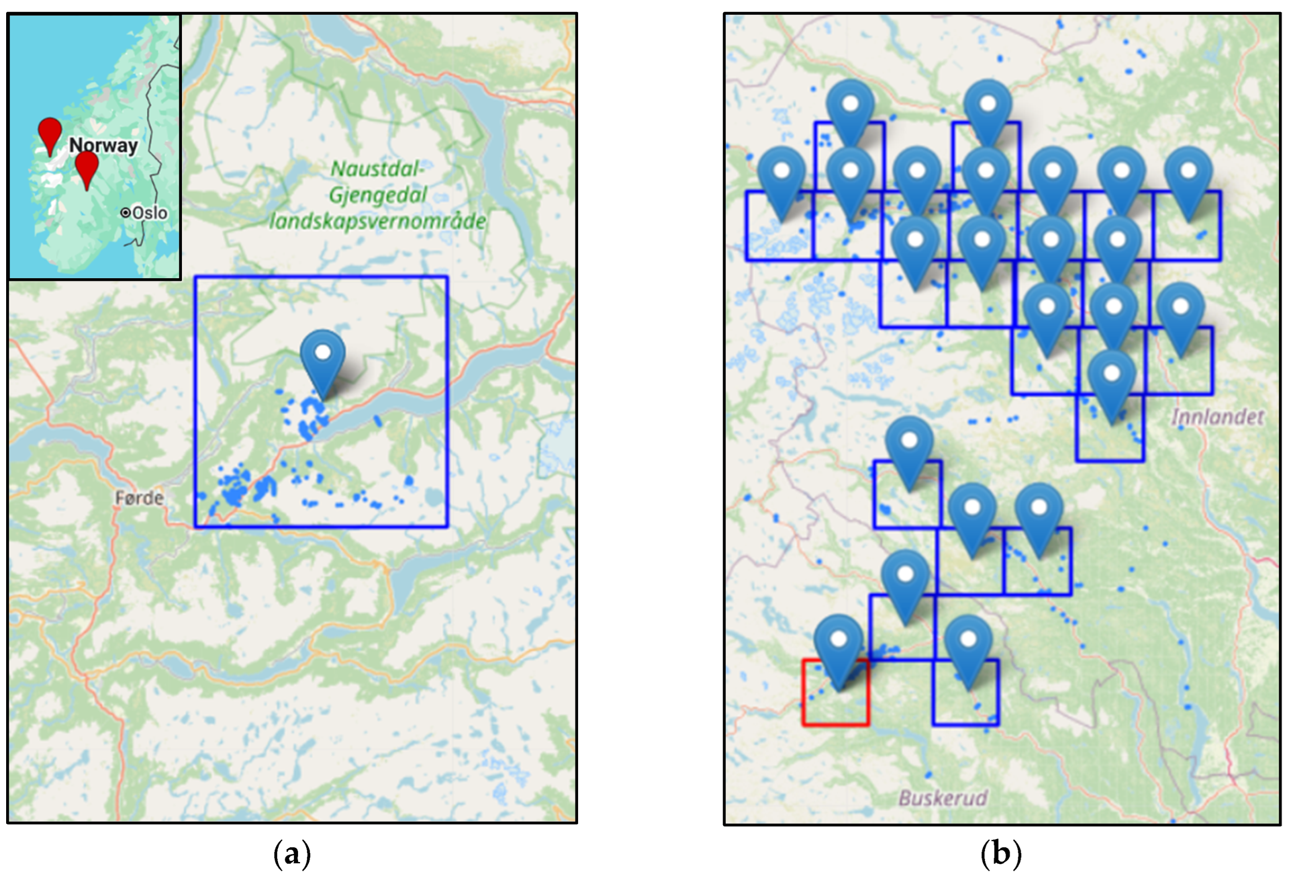
Figure 2.
Performance results from the Jølster test tile as a confusion image.
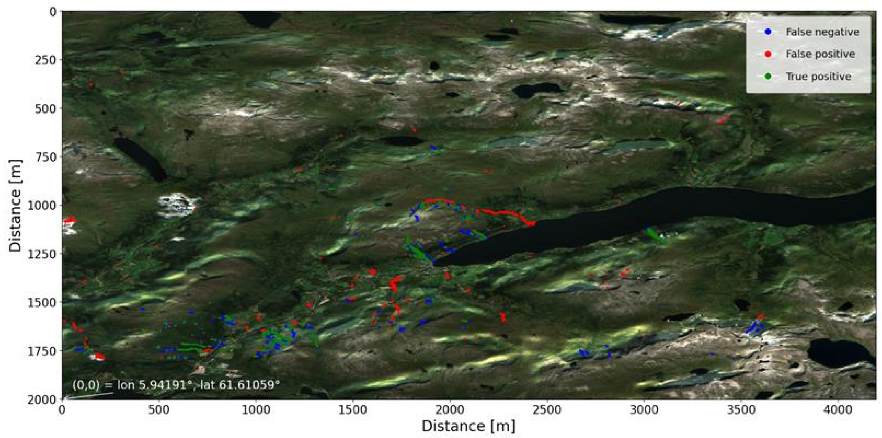
Figure 3.
Performance results from the Hans test tile as a confusion image.
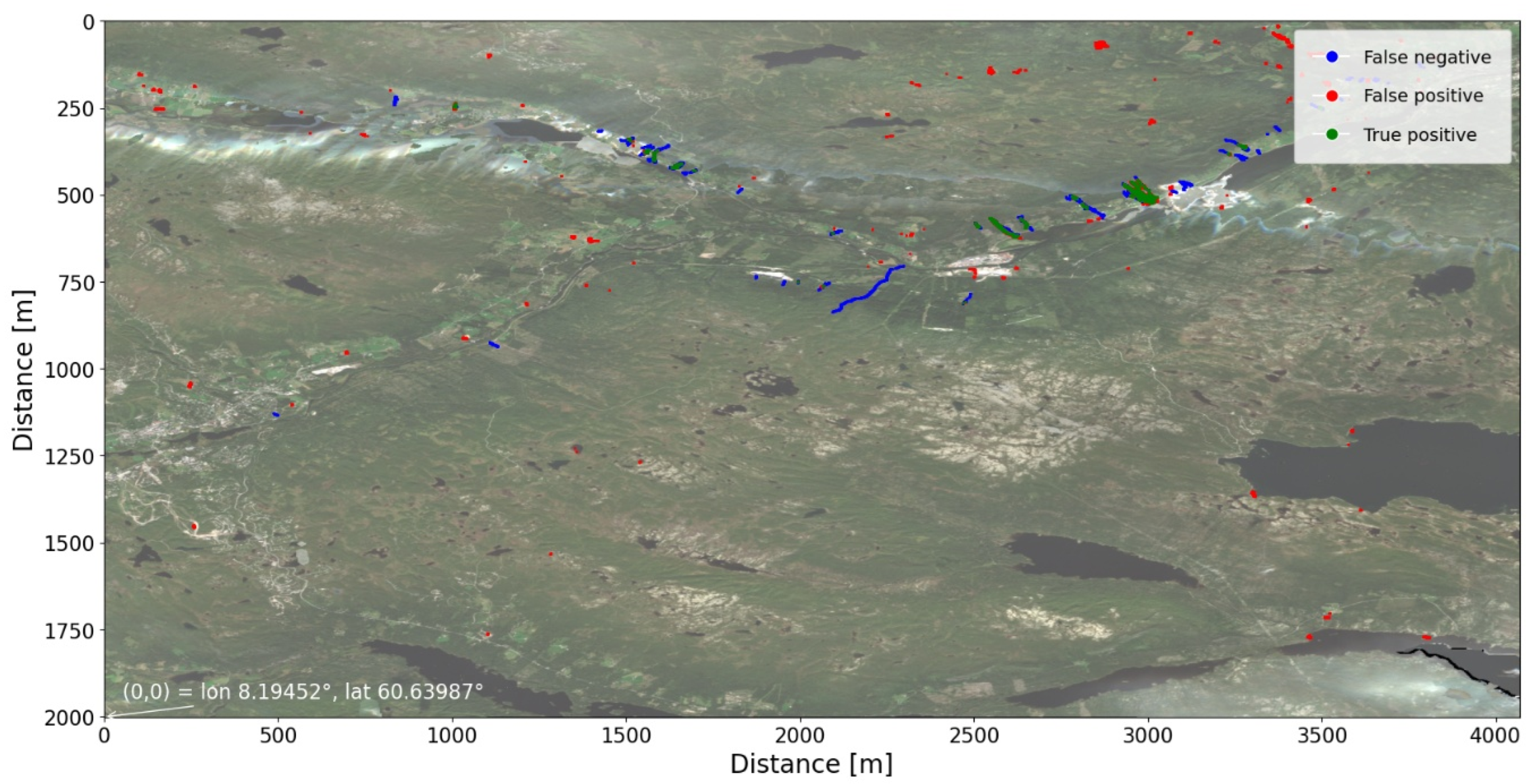
Figure 4.
Example from an excluded Hans tile showing false positives due to insufficient cloud filtering. The background image is a mosaic of the post-event images. Black shows areas with no data due to persistent cloud cover in the post-event period.
Figure 4.
Example from an excluded Hans tile showing false positives due to insufficient cloud filtering. The background image is a mosaic of the post-event images. Black shows areas with no data due to persistent cloud cover in the post-event period.
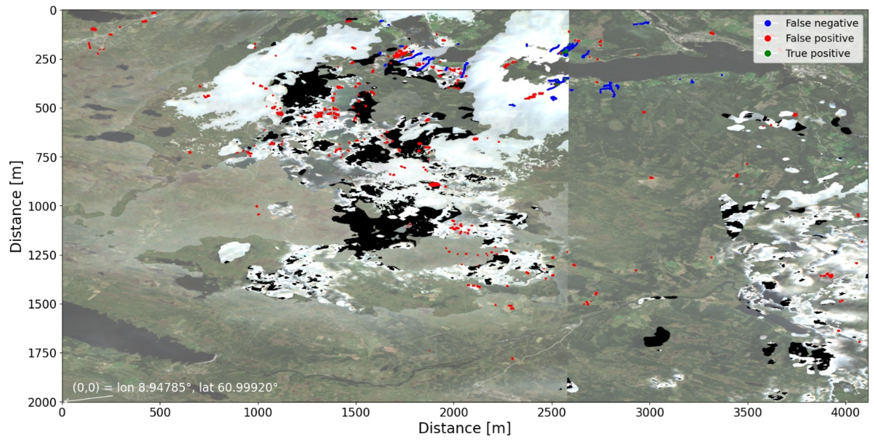
Figure 5.
Diagnostic plot shows false positives with the mass-transporting flood along the Svidalselva river predicted as a landslide. .
Figure 5.
Diagnostic plot shows false positives with the mass-transporting flood along the Svidalselva river predicted as a landslide. .
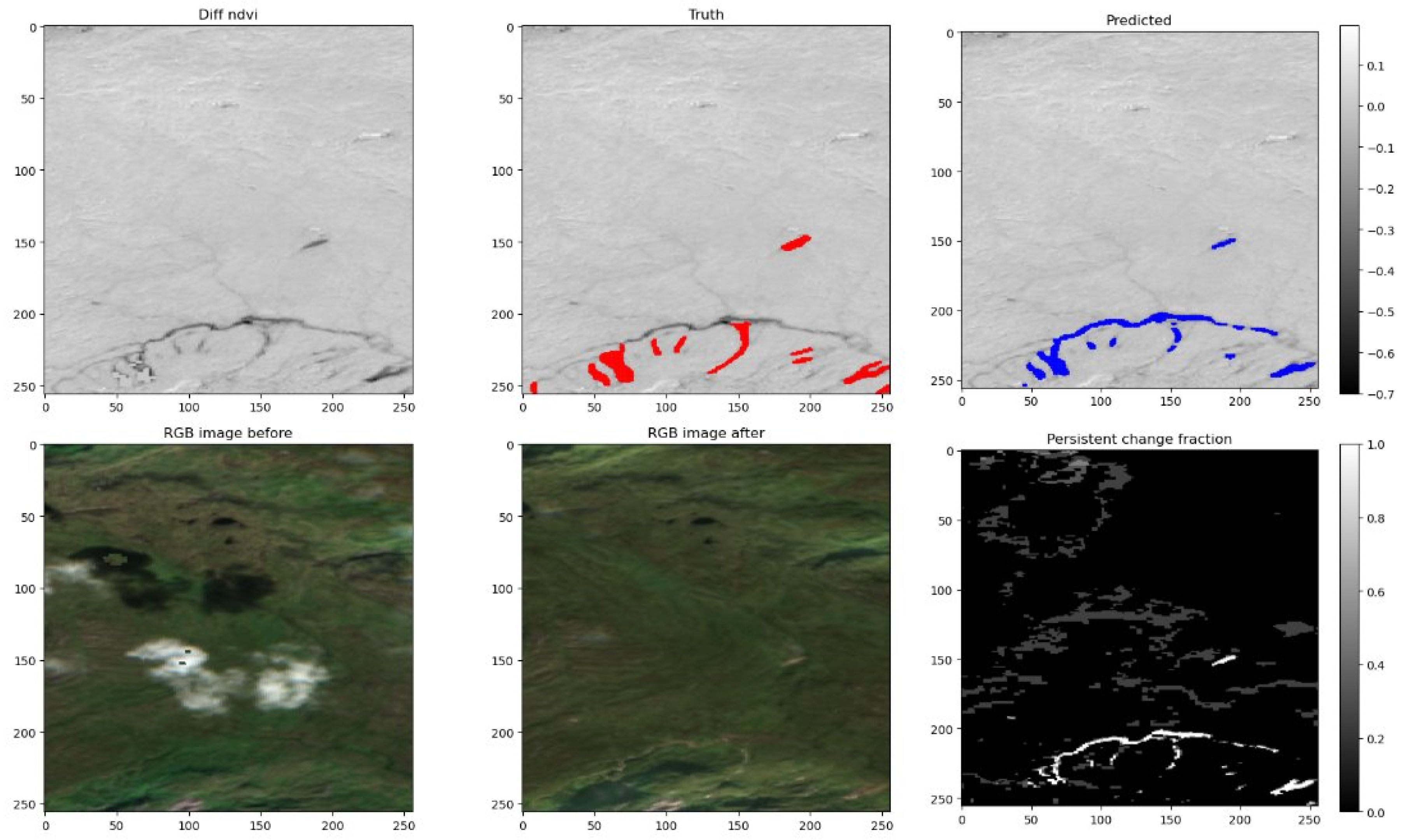
Figure 6.
Photos from a field visit to Jølster in October 2019: (a) deposits from a mass-transporting flood along Svidalselva river that were incorrectly predicted as a landslide by the model (false positive); (b) deposits from the large debris flow at Vassenden that terminated at the Western end of lake Jølster that were correctly predicted as a landslide (true positive).

Figure 7.
Diagnostic plot shows false negatives where there are small landslides that are not seen clearly in the Sentinel-2 images. Landslides with ID 42 and 43 are not visible.
Figure 7.
Diagnostic plot shows false negatives where there are small landslides that are not seen clearly in the Sentinel-2 images. Landslides with ID 42 and 43 are not visible.
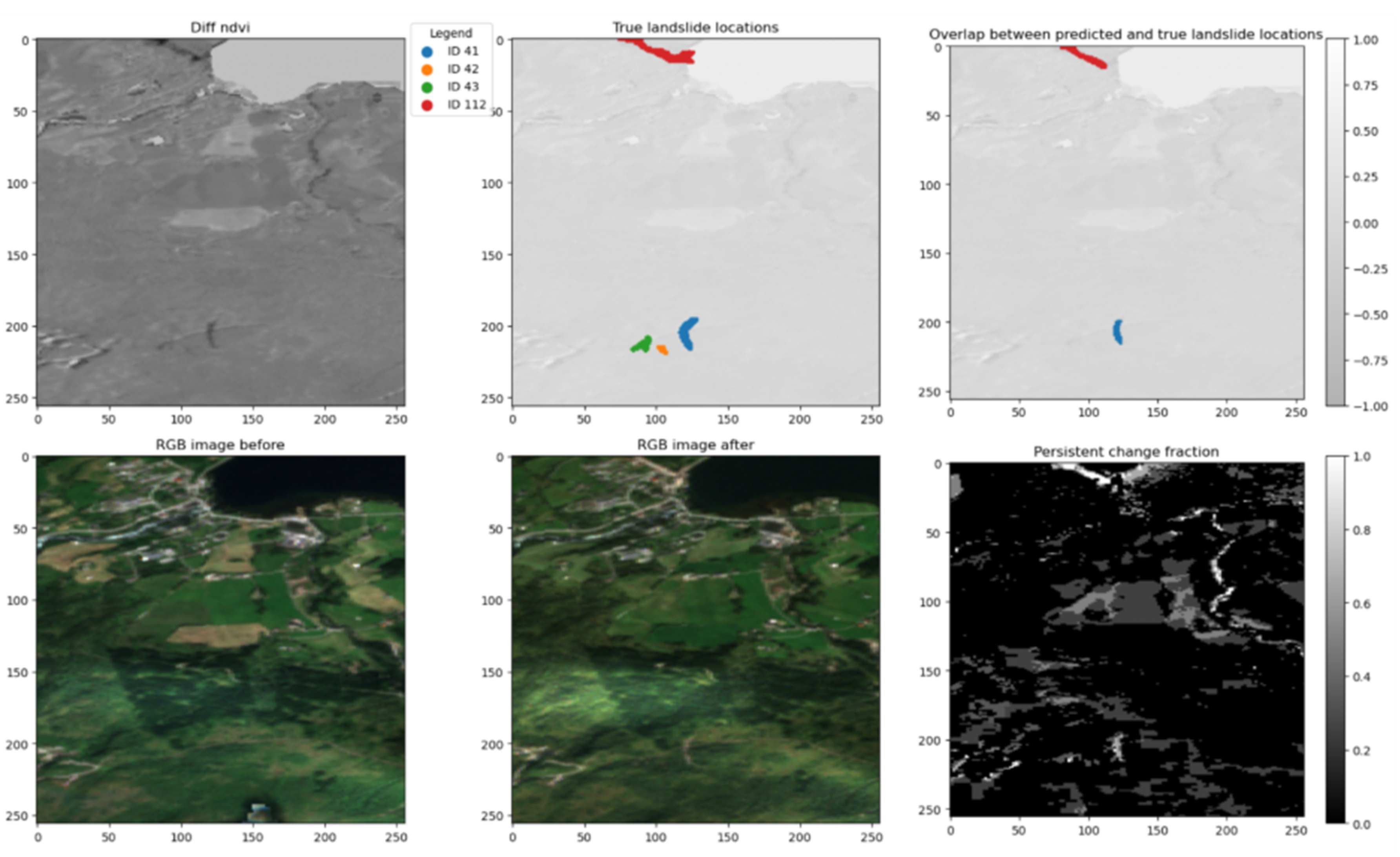
Figure 8.
Diagnostic plot shows landslides with ID 419 and ID 551 in the Hans area, that were only partially detected by the model, although expressed relatively clearly in the NDVI difference image.
Figure 8.
Diagnostic plot shows landslides with ID 419 and ID 551 in the Hans area, that were only partially detected by the model, although expressed relatively clearly in the NDVI difference image.
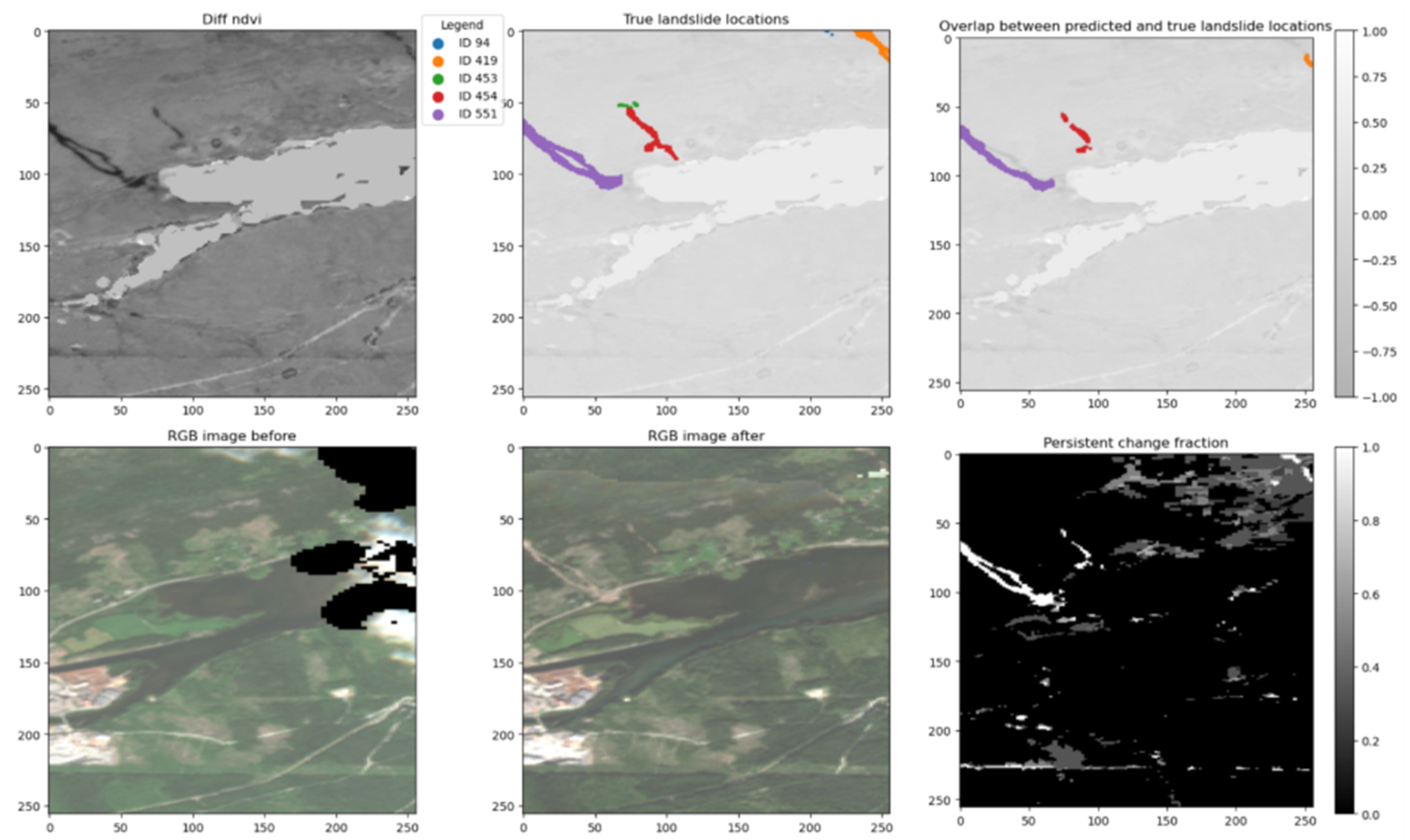
Figure 9.
Diagnostic plot shows landslides with ID 110, ID 9 and ID 7 in the Jølster area, that were missed or only partially detected by the model, although they are relatively clear in the NDVI difference image.
Figure 9.
Diagnostic plot shows landslides with ID 110, ID 9 and ID 7 in the Jølster area, that were missed or only partially detected by the model, although they are relatively clear in the NDVI difference image.
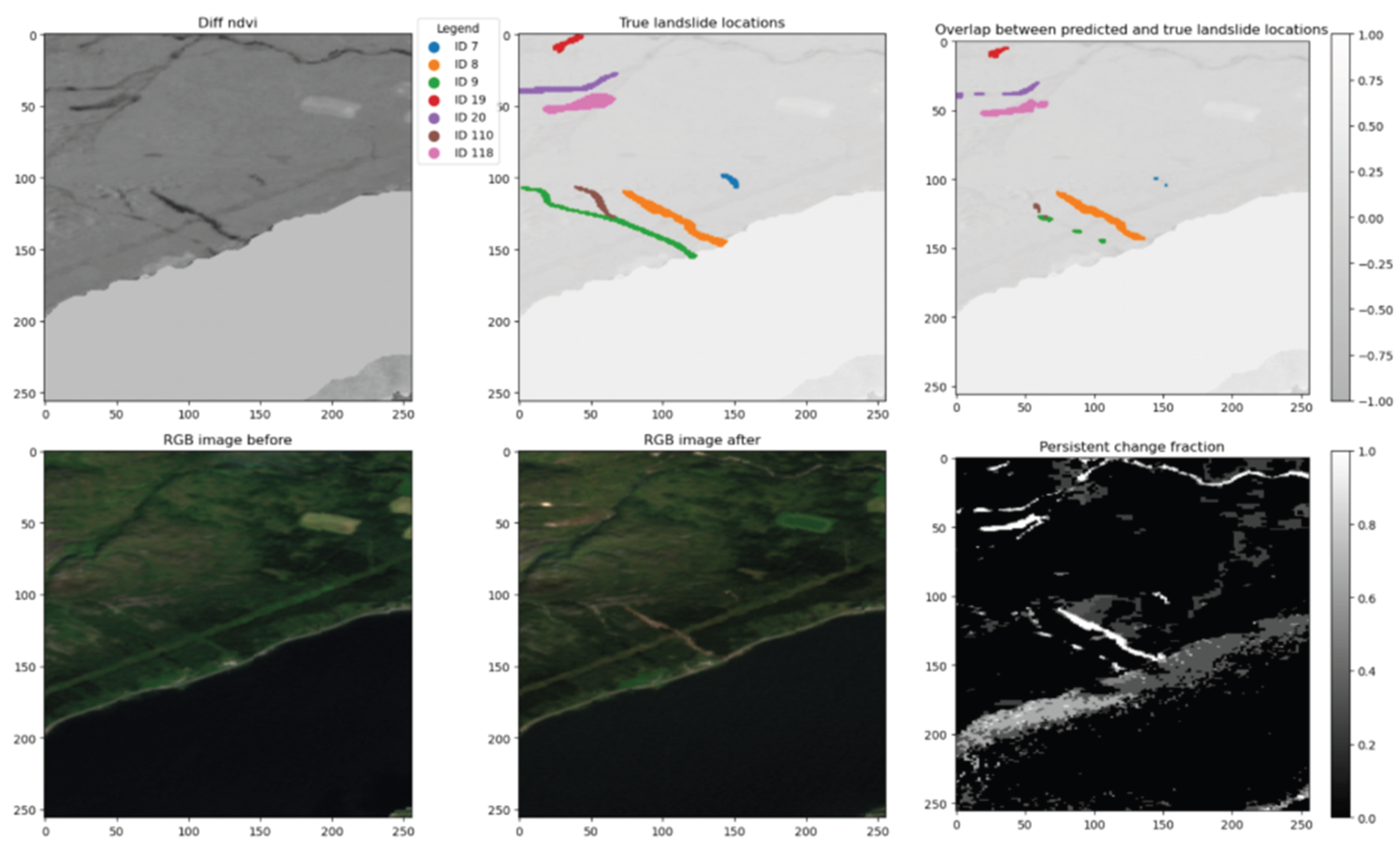

Table 1.
Model Performance for Jølster and Hans test areas.
| Results | Jølster | Hans |
|---|---|---|
| Total Landslides | 120 | 60 |
| At least 1 pixel overlap | 79 | 23 |
| At least 20% pixel overlap | 63 | 16 |
| Precision (%) | 53 | 35 |
| Recall (%) | 53 | 44 |
| Accuracy (%) | 99.8 | 99.9 |
| F1-score | 53 | 38.9 |
Disclaimer/Publisher’s Note: The statements, opinions and data contained in all publications are solely those of the individual author(s) and contributor(s) and not of MDPI and/or the editor(s). MDPI and/or the editor(s) disclaim responsibility for any injury to people or property resulting from any ideas, methods, instructions or products referred to in the content. |
© 2026 by the authors. Licensee MDPI, Basel, Switzerland. This article is an open access article distributed under the terms and conditions of the Creative Commons Attribution (CC BY) license (http://creativecommons.org/licenses/by/4.0/).
Copyright: This open access article is published under a Creative Commons CC BY 4.0 license, which permit the free download, distribution, and reuse, provided that the author and preprint are cited in any reuse.


