Submitted:
30 January 2026
Posted:
02 February 2026
You are already at the latest version
Abstract
Urban flood frequency analysis faces unique challenges as land development alters watershed hydrology, producing nonstationary flood records. This study demonstrates nonstationary flood frequency analysis (NSFFA) using RMC-BestFit, an open-source Bayesian software, through two Texas case studies. Brays Bayou at Houston (96 years of record) exemplifies an urbanized watershed with increasing flood trends; a step-logistic model captures both the abrupt increase in mean flood magnitude around 1968 and the progressive decrease in log-space variance as urbanization homogenized runoff response. O.C. Fisher Reservoir (169 years of record) exhibits decreasing trends attributed to brush encroachment and groundwater extraction; despite a sinusoidal model achieving best information criteria, a step function was selected based on physical reasoning, demonstrating that statistical fit alone should not dictate model selection. Results reveal contrasting frequency curve patterns: at O.C. Fisher, stationary and nonstationary curves differ uniformly (53\% reduction in 100-year flood), while at Brays Bayou, curves differ substantially for frequent events (48\% increase in 2-year flood) but converge in the extreme tail due to opposing trends in location and scale parameters. These findings underscore that NSFFA relevance depends on decision context. Bayesian methods offer key advantages including flexible integration of diverse data sources, comprehensive uncertainty quantification, and principled model comparison. Open-source software democratizes access to these methods, promoting transparency and reproducibility.
Keywords:
urban floods
; Bayesian analysis
; nonstationarity
; land use change
; uncertainty
; risk assessment
; open-source software
1. Introduction
Urban areas face disproportionate flood risks globally, with dense populations and critical infrastructure concentrated in floodplains. The Centre for Research on the Epidemiology of Disasters (CRED) reported that floods were the most common disasters worldwide in 2023, affecting several million people and causing over ten thousand deaths [1]. According to CRED, floods and severe storms (including tropical cyclones and convective events) accounted for more than 70% of natural disasters on average between 2003 and 2023. Urban areas experience particularly severe impacts due to concentrated development and hydrologic modifications. Furthermore, flood risk management infrastructure in the U.S. and globally is aging, making many existing structures vulnerable to the compounding impacts of climate change. Urban flood frequency analysis presents unique challenges as ongoing development fundamentally alters watershed runoff characteristics, producing flood records that violate the stationarity assumption underlying traditional frequency methods [2,3].
Both natural and anthropogenic influences can alter flood behavior over time. Conceptually, a warming climate increases the amount of precipitable water in the atmosphere, which could increase the likelihood of extreme floods. Conversely, land use changes such as agricultural intensification and groundwater extraction can reduce runoff generation in some watersheds. Therefore, incorporating climate change and land use evolution into flood hazard and risk analysis is crucial for dam and levee safety professionals, urban planners, and infrastructure managers.
Urbanization increases flood peaks through multiple mechanisms: expansion of impervious surfaces reduces infiltration capacity, channelization and drainage improvements increase conveyance efficiency, and loss of floodplain storage reduces attenuation [4]. These changes can be rapid, with urban watersheds experiencing order-of-magnitude increases in impervious cover over several decades. Consequently, flood frequency distributions estimated from historical data may poorly represent current or future conditions if temporal trends are not explicitly modeled [5,6].
1.1. The Stationarity Problem
Traditional flood frequency analysis assumes that flood magnitudes are independent and identically distributed samples from a stationary probability distribution [7]. This stationarity paradigm has been challenged as observational evidence increasingly demonstrates temporal nonstationarity in hydrologic extremes [2,8]. Bayazit [3] provided a comprehensive review of nonstationarity in hydrological records and methods for trend detection. For urban watersheds undergoing active development, the stationarity assumption is particularly problematic, as the watershed generating flood events today differs fundamentally from the watershed that produced historical flood observations.
Nonstationary flood frequency analysis (NSFFA) provides a framework for explicitly modeling temporally evolving flood risk. Rather than assuming constant distribution parameters, NSFFA allows location, scale, and shape parameters to vary with time or covariates [9,10,11]. Strupczewski et al. [9] introduced the foundational maximum likelihood framework for nonstationary at-site modeling. Recent advances have demonstrated various NSFFA approaches across multiple frameworks. Debele et al. [12,13] applied generalized additive models for location, scale, and shape (GAMLSS) parameters to Polish flood data. Cheng and AghaKouchak [14] developed nonstationary intensity-duration-frequency curves for precipitation extremes under climate change. Chen et al. [15] provided a comprehensive comparison of linear, nonlinear, parametric, and nonparametric regression models for NSFFA. Grego and Yates [16] recently introduced robust local likelihood estimation methods. Wasko et al. [17] provided a systematic review of climate change science relevant to Australian design flood estimation, including NSFFA approaches.
1.2. Bayesian Approaches to Flood Frequency Analysis
Bayesian methods have become increasingly prominent in flood frequency analysis due to their ability to incorporate prior information, quantify uncertainty comprehensively, and provide coherent probabilistic inference [18]. Foundational work by Kuczera [19,20] established Bayesian approaches for regional skew estimation and at-site flood frequency analysis using Monte Carlo methods. Reis and Stedinger [21] extended these methods to incorporate historical flood information through Markov Chain Monte Carlo (MCMC) sampling. Viglione et al. [22] developed a comprehensive Bayesian framework for flood frequency hydrology integrating multiple information sources. O’Connell et al. [23] demonstrated Bayesian analysis with paleohydrologic bound data, enabling incorporation of geologic evidence.
Regional Bayesian approaches have been developed to pool information across sites while accounting for spatial heterogeneity [24,25,26]. Kwon et al. [27] introduced climate-informed hierarchical Bayesian models for Montana flood frequency.
Bayesian approaches to NSFFA have been demonstrated by Renard et al. [10,28], Ouarda and El-Adlouni [29,30], Luke et al. [31], Xu et al. [32], and Bracken et al. [33]. Ouarda and El-Adlouni [30] provided a foundational discussion of Bayesian NSFFA with efficient estimation using generalized maximum likelihood methods. Bracken et al. [33] extended Bayesian hierarchical methods to multivariate nonstationary frequency analysis. International applications include Bossa et al. [34] in West Africa and Xiong et al. [35] analyzing 547 years of Yangtze River flood records under nonstationarity.
Despite these methodological advances, practical application of Bayesian NSFFA remains limited in engineering practice due to software availability, computational complexity, and challenges in selecting appropriate trend structures from numerous possible models.
1.3. Model Selection for Nonstationary Analysis
Model selection presents a critical challenge in both stationary and nonstationary flood frequency analysis. Di Baldassarre et al. [36] and Laio et al. [37] developed comprehensive frameworks for comparing candidate probability distributions using information criteria including AIC and BIC. Haddad and Rahman [38] demonstrated distribution and parameter estimation selection in Australian applications.
For nonstationary analysis, model selection must additionally address trend structure complexity. Parsimonious approaches are essential to avoid overfitting, particularly given typically limited flood record lengths. Serago and Vogel [39] introduced parsimonious NSFFA methods emphasizing the importance of balancing model complexity with predictive performance. Singh et al. [40] developed a diagnostic framework for comparing stationary and nonstationary analyses under changing climate.
1.4. RMC-BestFit Software
The U.S. Army Corps of Engineers (USACE) Risk Management Center developed RMC-BestFit as a Bayesian estimation and fitting software designed to enhance flood hazard assessments [41,42]. The software implements a comprehensive Bayesian framework that can incorporate multiple sources of hydrologic information including systematic streamflow data, historical flood records, paleoflood indicators, regional rainfall-runoff analyses, and expert elicitation [22,43,44].
RMC-BestFit employs MCMC methods to sample from posterior distributions of distribution parameters, providing full characterization of parameter uncertainty. The Differential Evolution Markov Chain with snooker update (DE-MCzs) algorithm [45] enables efficient exploration of complex posterior distributions. Recent enhancements include NSFFA capabilities allowing distribution parameters to vary with time through flexible trend functions: linear, polynomial, exponential, logistic, power, sinusoidal, and step functions. Model selection tools based on Akaike Information Criterion (AIC), Bayesian Information Criterion (BIC), and Deviance Information Criterion (DIC) help identify parsimonious trend structures balancing goodness-of-fit with complexity [37,38].
The software is freely available as open-source code on GitHub (https://github.com/USACE-RMC/RMC-BestFit), promoting transparency, reproducibility, and community development.
1.5. Objectives
This study demonstrates practical application of Bayesian NSFFA using RMC-BestFit through two contrasting case studies from Texas watersheds. The first case study examines Brays Bayou at Houston, one of the most intensively urbanized watersheds in the United States, where 96 years of flood data (1929–2024) including threshold-censored historical information reveal increasing trends in flood magnitude accompanied by decreasing variance as urbanization homogenized the watershed’s runoff response. The second case study analyzes O.C. Fisher Reservoir, where 169 years of historical and systematic data (1853–2021) show decreasing trends attributed to brush encroachment and groundwater extraction.
The objectives are to: (1) outline the Bayesian NSFFA methodology and suite of trend options implemented in RMC-BestFit; (2) demonstrate model selection procedures using multiple information criteria while emphasizing the critical role of physical reasoning; (3) evaluate how changes in both location and scale parameters interact to produce different patterns of difference between stationary and nonstationary frequency curves; (4) illustrate how the relevance of NSFFA depends on decision context (frequent events versus extreme events); and (5) provide practical guidance on trend model selection for different watershed types and nonstationarity mechanisms.
2. Materials and Methods
2.1. Likelihood Function
A key component of Bayesian flood frequency analysis is the likelihood function, which gives the probability of the observed data conditional on the distribution parameters [20]. For stationary analysis with exact (systematic) data only, the likelihood is:
where is the sample of observed annual maximum flows, represents the constant distribution parameters, and is the probability density function.
2.2. Nonstationary Likelihood Function
When distribution parameters vary with time, each observation at time t follows a distribution with time-dependent parameters [9,30]. The nonstationary likelihood becomes:
The likelihood can be extended to accommodate various data types commonly encountered in flood frequency analysis [20,21,23,46]:
where is the probability density function, is the cumulative distribution function, and superscripts U and L denote upper and lower bounds for censored observations. Left censoring indicates the observation is known to be below a threshold but the exact magnitude is unknown; right censoring indicates the observation exceeded a threshold. This flexibility allows incorporation of historical flood information following the foundational work of Stedinger and Cohn [47], as demonstrated by Xiong et al. [35] for multi-century flood records.
2.3. Bayesian Framework and Prior Information
In the Bayesian approach to flood frequency analysis, distribution parameters (representing location (), scale (), and shape ()) are treated as random variables rather than fixed constants [18,20]. This conceptualization enables explicit quantification of parameter uncertainty arising from limited data.
Bayesian inference combines observed data with prior information through Bayes’ theorem [20]:
where is the posterior probability distribution of the parameters given the observed data, is the likelihood function, is the prior distribution encoding information available before analyzing the current data, and the denominator serves as a normalizing constant.
The prior distribution is not derived from the observed flood data, but instead comes from other sources that can be either subjective (e.g., expert opinion) or objective (e.g., regional analysis, previous studies). This prior information is particularly valuable for constraining parameters that are poorly informed by limited data.
2.3.1. Prior Information on Parameters
Prior information for distribution parameters can include regional hydrologic knowledge [19,24], paleoflood evidence [23], or information from analogous watersheds. RMC-BestFit automatically develops default priors to ensure ease of use while maintaining statistical rigor. Flat (uniform) priors are applied to all distribution parameters (location, scale, and shape), centered near the likelihood with broad spread to remain relatively uninformative. Additionally, a Jeffreys’ prior is applied to the scale parameter by default, which provides appropriate behavior for positive-valued parameters and is equivalent to using a log-link function. Users can override these defaults with informative priors when regional or prior knowledge is available. While flat priors yield posterior inference that approximates maximum likelihood results for well-identified parameters, the Bayesian framework retains key advantages: proper uncertainty quantification through the full posterior distribution rather than asymptotic approximations, natural handling of complex likelihoods with censored data types, and posterior predictive distributions that integrate parameter uncertainty.
The joint prior probability of model parameters is given by:
where p is the number of parameters. In RMC-BestFit, parameters are treated as independent, so the joint prior simplifies to:
where is the probability density function for each parameter’s prior distribution.
2.3.2. Prior Information on Quantiles
Viglione et al. [22] presented a framework for incorporating causal information from rainfall-runoff modeling or regional analysis through quantile priors. Causal information expansion analyzes the generating mechanisms of floods in the catchment and is typically derived using rainfall-runoff models or expert elicitation.
A quantile prior specifies the distribution of a flood magnitude corresponding to a specific annual exceedance probability p:
where is a probability density function for the quantile prior and represents the hyperparameters of the chosen prior distribution (e.g., mean and standard deviation). RMC-BestFit supports several distribution options for quantile priors including Normal, Log-Normal, and Truncated Normal, allowing users to select the form most appropriate for their prior information. The flood quantile relates to distribution parameters through the inverse cumulative distribution function:
where are the distribution parameters at the final time step. The inverse CDF is then used to evaluate the quantile prior in parameter space:
During MCMC sampling, the quantile prior acts as a penalty function, rewarding parameter sets that produce flood quantiles consistent with the prior information and discounting those that do not. The complete posterior distribution combines all information sources:
This framework allows systematic integration of multiple data types: at-site observations through the likelihood, regional parameter knowledge through parameter priors, and rainfall-runoff or climate projection results through quantile priors.
RMC-BestFit also implements quantile priors following the method of Coles and Tawn [44], which provides a more complete mathematical treatment allowing multiple quantile priors to be specified simultaneously. This approach requires that the number of quantile priors equals the number of distribution parameters; for a three-parameter distribution such as Log-Pearson Type III, exactly three quantile priors must be specified (e.g., at the 0.10, 0.01, and 0.001 exceedance probabilities). The O.C. Fisher case study demonstrates this approach using quantile priors derived from rainfall-runoff modeling.
Critical for nonstationary analysis: Prior distributions on parameters and quantiles are applied at the final time step T (representing current or future conditions). This ensures that prior knowledge about current flood behavior appropriately constrains the temporal evolution of the distribution through the trend functions [22]. The trend parameters themselves (slopes, change points, etc.) typically receive uninformative priors.
2.3.3. Incorporating Climate Projections
Global Climate Model (GCM) projections can be incorporated into Bayesian NSFFA through quantile priors in RMC-BestFit. For sites where climate projections indicate continued changes in runoff, the mean flows of quantile priors ( in Equation 7) can be adjusted accordingly to reflect projected future conditions. This approach provides a principled mechanism for integrating climate science with flood frequency analysis, supporting forward-looking infrastructure planning decisions.
2.4. Detecting Nonstationarity
Detecting changes in the time series data is a critical first step in NSFFA. A nonstationary time series will often exhibit a trend or jump that can be increasing or decreasing and may be linear or nonlinear. The cause of the nonstationarity can be gradual changes in hydrological and climatological factors, or anthropogenic changes such as alterations in land use and land cover.
RMC-BestFit provides several widely used hypothesis tests for evaluating flood series properties [48,49]. Some tests assess whether the independence and identical distribution (i.i.d.) assumptions are satisfied, while others specifically detect nonstationarity. These include:
- Jarque-Bera test for detecting departures from normality [50];
- Ljung-Box Q test for autocorrelation indicating periodicity [51];
- Mann-Whitney U test for differences in distribution between subperiods [55];
- Linear regression trend test for slope significance [48];
- Student’s t-test (equal and unequal variance) for differences in means between subperiods [58];
- F-test for differences in variance between subperiods [58];
- Mixture model test for unimodality versus multimodal distributions [59].
Table 2 and Table 5 present hypothesis test results for the two case study watersheds. Multiple tests rejecting the null hypothesis of stationarity, combined with visual inspection of flood chronology plots showing clear patterns, provide strong motivation for nonstationary modeling.
The autocorrelation function (ACF) provides additional insight into the nature of nonstationarity and informs trend model selection. Persistent positive autocorrelation with slow exponential decay indicates a strong monotonic trend, while oscillatory ACF patterns with peaks at specific lags may suggest periodicity, though such patterns can also arise as artifacts of abrupt regime shifts combined with sampling variability. ACF analysis for each case study is presented alongside hypothesis test results in Section 3.
2.5. Return Period Interpretation and Risk Communication Under Nonstationarity
The interpretation of return periods and risk under nonstationary conditions requires careful reconsideration of traditional concepts. Read and Vogel [60] provided comprehensive analysis of reliability, return periods, and risk under nonstationarity, demonstrating that traditional return period interpretations become problematic when exceedance probabilities vary with time. Their subsequent work [61] introduced hazard function analysis and reliability-based methods as alternative frameworks for flood planning under nonstationary conditions.
This study employs a complementary approach based on the “Time Index” concept [14], which provides annual exceedance probability (AEP) inference conditioned on a specific time step rather than computing time-integrated reliability measures. Since distribution parameters vary with time in NSFFA, the exceedance probability and corresponding return period of a flow value also varies with time. In a stationary frequency analysis, the return period provides a straightforward and consistent measure of the likelihood of an event occurring. For example, a flood with a return period of 100 years has a 1% chance of being exceeded in any given year.
However, in nonstationary frequency analysis where statistical properties change over time, the concept of a return period becomes more complex. The return period can vary over time, reflecting the changing probabilities of event magnitudes [60]. Consequently, the return period in a nonstationary analysis must be carefully interpreted, often focusing on specific time steps or conditions to provide meaningful insights.
The Time Index approach determines which time step to use for evaluating the nonstationary frequency distribution [14]. For dam and levee safety applications, risk is typically evaluated using current conditions rather than forecasted or hindcasted conditions. Thus, parameters from the most recent time step are used for flood hazard prediction in risk analysis, providing AEP estimates conditional on present-day watershed conditions. However, users can choose any time step within the study period and forecast into the future to support scenario-based planning decisions [62]. This time-conditioned AEP inference differs from reliability-based methods [60,61] but provides a practical framework for engineering applications where decisions are based on current or projected future conditions. Application of this approach is demonstrated in the case study results (Section 3).
2.6. Trend Model Formulations
RMC-BestFit implements multiple trend model options for location, scale, and shape parameters. In practice, insufficient data typically precludes reliable estimation of time-varying shape parameters, so trend modeling focuses primarily on location and occasionally scale parameters [30,62]. Serago and Vogel [39] emphasized the importance of parsimony in trend model selection.
Table 1 summarizes trend model options with typical use cases relevant to hydrology and flood frequency analysis.
2.7. Probability Distribution Selection
The Log-Pearson Type III (LP3) distribution was selected for both case studies presented in this paper, consistent with federal guidelines established in Bulletin 17C [7]. The LP3 distribution has been the standard for flood frequency analysis in the United States since 1967 and remains the recommended distribution for federal agencies. This distribution is particularly well-suited for modeling flood data because it: (1) accommodates the positive skewness typically observed in flood records, (2) provides flexibility through three parameters (location, scale, and shape), and (3) has been extensively validated across diverse hydrologic regimes.
In RMC-BestFit’s implementation, the LP3 distribution is fit to the logarithms of annual maximum flows. For nonstationary analysis, the location () and scale () parameters can vary with time according to specified trend functions, while the shape parameter (skewness) is typically held constant due to data limitations for reliable estimation of time-varying skewness [30,62]. While RMC-BestFit supports multiple probability distributions (Generalized Extreme Value, Generalized Logistic, Normal, etc.), the LP3 was selected here to maintain consistency with standard practice and facilitate comparison with conventional stationary analyses.
2.8. Model Selection Using Multiple Criteria
Selecting appropriate trend structures presents a critical challenge in NSFFA [37,39]. RMC-BestFit implements three information criteria:
Akaike Information Criterion (AIC):
Bayesian Information Criterion (BIC):
2.9. Posterior Inference
RMC-BestFit employs MCMC methods using the DE-MCzs algorithm [45] to sample from the posterior distribution. Xu et al. [32] demonstrated adaptive Metropolis-Hastings optimization for Bayesian NSFFA.
The posterior predictive distribution integrates over parameter uncertainty to characterize the distribution of future floods [22]:
This distribution accounts for both parameter uncertainty (epistemic) and natural variability (aleatory), providing comprehensive uncertainty quantification essential for risk-informed decision making [20,63]. This Bayesian formulation has conceptual parallels to the expected probability distribution, which has a long history in U.S. flood frequency analysis for incorporating parameter uncertainty into quantile estimates [64,65].
The 90% credible intervals reported in this study are derived from the posterior predictive distribution, capturing both parameter uncertainty and natural variability. These intervals provide a probabilistic range within which future flood quantiles are expected to fall, given the observed data and model assumptions.
2.10. Practical Implementation for Engineering Applications
While Bayesian MCMC methods are mathematically sophisticated, RMC-BestFit is designed to shield practitioners from implementation complexity, allowing engineers to focus on hydrologic interpretation rather than computational details. Key features enabling practical application include:
Automatic Prior Generation: The software automatically constructs default priors based on the observed data range and distribution support, enabling immediate use without requiring prior specification. Flat priors are applied to location, scale, and shape parameters, with an additional Jeffreys’ prior on the scale parameter. Users can optionally specify informative priors when regional or causal knowledge is available.
Adaptive Sampling: The DE-MCzs algorithm automatically adapts proposal distributions during burn-in, removing the need for manual tuning of step sizes and acceptance rates that traditionally require MCMC expertise.
Convergence Diagnostics: Built-in diagnostics (Gelman-Rubin statistics, effective sample size, trace plots) are computed automatically, alerting users to potential convergence issues without requiring interpretation of raw MCMC output.
Default Settings: Recommended chain lengths, burn-in periods, and thinning intervals are provided as defaults, based on extensive testing across diverse flood datasets.
Graphical Interface: The user interface guides workflow from data import through model specification, estimation, and results visualization, requiring no programming or scripting knowledge.
These features enable engineers familiar with traditional flood frequency analysis to apply Bayesian NSFFA methods without specialized statistical training, democratizing access to advanced uncertainty quantification approaches.
3. Results
The following case studies are presented holistically, integrating watershed description, data characteristics, and frequency analysis results for each site to maintain narrative coherence. This organization follows the case study presentation format common in applied flood hydrology literature.
3.1. Case Study Watersheds
This study examines two watersheds in Texas selected to represent contrasting nonstationary behaviors relevant to urban flood management. Case Study 1 (Brays Bayou, Houston) represents a heavily urbanized watershed exhibiting increasing flood trends resulting from rapid land use conversion, following the analytical framework demonstrated by Villarini et al. [5]. Case Study 2 (O.C. Fisher Reservoir, west Texas) represents a watershed with decreasing flood trends attributed to brush encroachment, groundwater extraction, and climate variability.
3.2. Case Study 1: Brays Bayou at Houston, Texas
The first case study examines Brays Bayou, a major urban waterway in southwest Houston that exemplifies the flood challenges facing rapidly urbanizing watersheds. Annual maximum streamflow data were obtained from USGS gage 08075000 (Brays Bayou at Houston, TX), located near the Main Street Bridge in Harris County. The drainage area upstream of the gage is approximately 246 km2 (94.9 mi2).
3.2.1. Flood Data
The systematic record spans water years 1936–2024, providing 89 years of continuous annual maximum instantaneous streamflow data. In addition to the systematic record, a significant flood event occurred in 1929 and was included as exact (uncensored) historical data. For the intervening period 1930–1935, a perception threshold of 994 m3/s was applied, indicating confidence that no flood during this six-year period exceeded the magnitude of the 2017 Hurricane Harvey event (the largest flood in the systematic record). This threshold-censored treatment follows established methods for incorporating historical information into flood frequency analysis [21,47].
The resulting dataset comprises 90 exact observations (1929 plus 1936–2024) and 6 threshold-censored years (1930–1935), spanning a total of 96 years. The combination of systematic and historical data substantially improves parameter estimation, particularly for the upper tail of the frequency distribution [47]. Figure 1 presents the flood chronology, illustrating the clear increasing trend associated with urbanization.
3.2.2. Watershed Characteristics
Brays Bayou is a principal tributary of Buffalo Bayou, flowing approximately 50 km (31 mi) from the western edge of Harris County, south of Barker Reservoir near the Fort Bend County border, eastward to its confluence with Buffalo Bayou at Harrisburg. The stream corridor traverses some of Houston’s most densely developed neighborhoods and districts, including Meyerland, Braeswood Place, the Texas Medical Center, and Riverside Terrace.
The Brays Bayou watershed represents one of the most intensively urbanized drainage basins in the United States. The broader watershed encompasses approximately 334 km2 (129 mi2) and supports a population exceeding 700,000 residents. The drainage network includes over 200 km (124 mi) of open-channel waterways, the majority of which are artificial drainage channels constructed to convey stormwater through the urban landscape. This combination of high population density, extensive impervious surface coverage, and limited flood control infrastructure renders Brays Bayou exceptionally susceptible to flash flooding.
3.2.3. Urbanization History
Urbanization within the Brays Bayou basin, consistent with broader Houston metropolitan development patterns, accelerated dramatically during the mid-20th century. Post-World War II population growth, successive petroleum industry expansions, and the emergence of the Houston Ship Channel as a major industrial corridor drove rapid conversion of agricultural and natural lands to urban uses. The most intensive development occurred between the 1970s and 2010s, during which impervious surface coverage increased substantially as residential subdivisions, commercial centers, and transportation infrastructure replaced permeable landscapes.
This transformation fundamentally altered watershed hydrology. Natural infiltration capacity diminished as concrete, asphalt, and rooftops replaced vegetated surfaces, while channelization projects increased conveyance efficiency but reduced floodplain storage. The combined effect has been a progressive increase in flood peaks and volumes for storms of equivalent magnitude, providing strong physical justification for nonstationary flood frequency analysis [5,6].
Houston’s flood history includes several catastrophic events that underscore the region’s vulnerability, including Tropical Storm Allison (2001) and Hurricane Harvey (2017). The watershed’s urban development timeline coincides with observed increases in flood frequency and magnitude, motivating explicit modeling of temporal trends in flood risk.
3.2.4. Hypothesis Testing
Table 2 presents hypothesis test results for the Brays Bayou annual maximum flow series. All trend tests reject the null hypothesis of stationarity at the level. The significant F-test () indicates changing variance between early and late periods, while the mixture model test confirms multimodality, consistent with distinct pre- and post-urbanization flow regimes.

Table 2.
Hypothesis test results for Brays Bayou at Houston.
| Test | Null Hypothesis | p-value | Sig. |
|---|---|---|---|
| Jarque-Bera | Normality | 0.0015 | ** |
| Ljung-Box Q | No autocorrelation | <1E-15 | *** |
| Wald-Wolfowitz | Independence/stationarity | 1.84E-10 | *** |
| Mann-Whitney U | Homogeneity/stationarity | 4.55E-11 | *** |
| Mann-Kendall | No monotonic trend | 1.33E-13 | *** |
| Linear Trend (slope) | <1E-15 | *** | |
| Equal Variance t-test | 4.23E-13 | *** | |
| Unequal Variance t-test | 5.91E-12 | *** | |
| F-test | 8.76E-07 | *** | |
| Mixture Model | Unimodality | 0.0004 | *** |
Significance codes: *** ; ** ; * ; ·.
The autocorrelation function (Figure 2) exhibits persistent positive autocorrelation with slow exponential decay, characteristic of a strong monotonic trend. This pattern, combined with the highly significant trend tests, confirms that nonstationarity must be explicitly modeled.
3.2.5. Model Estimation and Selection
Given the strong evidence for nonstationarity in both mean and variance (Table 2), seven candidate models were evaluated using the Log-Pearson Type III distribution. The significant F-test () and multimodal mixture test results motivated testing trend models on both location () and scale () parameters. Candidate models included: (1) stationary (constant parameters); (2) linear trend on ; (3) logistic trend on ; (4) step function on ; (5) linear on with logistic on ; (6) logistic on with logistic on ; and (7) step function on with logistic on .
Table 3 presents model comparison results. The logistic-logistic model achieved the lowest AIC and BIC values, while the step-logistic model (step function on , logistic on ) achieved the lowest DIC. Given that DIC is specifically designed for Bayesian model comparison and the step function provides an identifiable change point with clear physical interpretation, the step-logistic model was selected.
The step-logistic model is also physically compelling. The estimated mean change point of 1968 corresponds closely to the onset of Houston’s most intensive urbanization period in the early 1970s, when post-war suburban expansion accelerated dramatically. Notably, the logistic trend on the scale parameter indicates decreasing variance in log-space over time (negative slope ). While this may seem counterintuitive given the visually apparent spread of flows in recent years, examination of the log-transformed data reveals that early-period floods spanned over one order of magnitude (approximately 20–300 m3/s), whereas the post-urbanization period shows roughly half an order of magnitude spread (approximately 200–800 m3/s).
This decreasing log-space variance has a compelling physical interpretation: urbanization homogenizes the watershed’s runoff response. In the pre-development era, flood magnitudes were highly sensitive to antecedent soil moisture, vegetation state, and seasonal factors. Wet years produced dramatically different responses than dry years. As impervious surfaces came to dominate the watershed, these natural sources of variability diminished. A heavily urbanized watershed produces a more consistent, predictable (though higher magnitude) flood response regardless of antecedent conditions, because runoff generation is controlled primarily by impervious area rather than infiltration-dependent processes.
Figure 3 illustrates the fitted trends for four representative models, showing the time-varying 2-year flood (median annual maximum): (a) stationary baseline, (b) linear–logistic, (c) logistic–logistic, and (d) the selected step–logistic model. The step–logistic model captures both the abrupt increase in mean flood magnitude around 1968 and the progressive reduction in flood variability as urbanization homogenized the watershed response.
3.2.6. Frequency Analysis Results
Table 4 presents flood quantile estimates comparing stationary and nonstationary analyses using current conditions (2024). A notable feature of the Brays Bayou results is the convergence of stationary and nonstationary frequency curves in the extreme right tail, with the largest differences occurring for frequent events. This convergence pattern arises from the opposing trends in location (increasing) and scale (decreasing) parameters, with implications for practice discussed in Section 4.2.
The quantitative differences are substantial for frequent events but diminish toward the tail. The 2-year flood is 48% larger under the nonstationary model (511 versus 346 m3/s), and the 5-year flood is 9% larger (661 versus 607 m3/s). However, differences diminish rapidly: the 10-year floods are nearly identical (749 versus 744 m3/s, less than 1% difference), and the 100-year floods are essentially equivalent (996 versus 993 m3/s). This convergence pattern contrasts sharply with O.C. Fisher, where uniform differences occur across all return periods.
Figure 4 presents the flood frequency curves comparing stationary and nonstationary analyses. The convergence of curves in the extreme tail is clearly visible, with substantial differences for frequent events.
3.3. Case Study 2: O.C. Fisher Reservoir, West Texas
O.C. Fisher Dam is located on the North Concho River in west Texas with a catchment area of approximately 3,885 km2. Period-of-record systematic inflows were obtained from 1916 to 2021, providing 106 years of annual maximum 2-day average inflow data. The largest flood during the systematic period occurred on September 17, 1936, and was estimated to be approximately 1,150 m3/s.
The observed decline in flood magnitudes at O.C. Fisher coincides with significant changes in the North Concho watershed during the mid-20th century. Progressive encroachment of mesquite and juniper, which accelerated from the late 1800s through the 1950s due to overgrazing and fire suppression, fundamentally altered watershed hydrology [66]. These deep-rooted woody plants intercept precipitation through transpiration, depleting soil moisture and reducing aquifer recharge. Concurrently, agricultural irrigation pumping from the Edwards-Trinity aquifer lowered regional water tables, with documented declines exceeding 100 feet in portions of the watershed between the 1930s and 1960s. These combined effects depleted shallow aquifers that historically fed springs, converting perennial streams to intermittent channels. The Upper Colorado River Authority documented that streamflow at Carlsbad decreased to less than 22% of pre-1960 levels despite slightly increased rainfall [66].
Based on historical records and reports, the largest flood on the North Concho River occurred in 1853 and was at least as large as the 1936 event. Multiple other large events occurred between 1854 and 1915, but none exceeded the 1936 flood magnitude. In RMC-BestFit, the historical period from 1853 to 1915 was treated as binomial-censored following methods established by Stedinger and Cohn [47], where data points during this period have magnitudes known to be below a threshold value, with one flood (1853) known to exceed the threshold, but exact magnitudes are unknown. This treatment has been extended to nonstationary contexts by Machado et al. [46] and Xiong et al. [35]. The resulting dataset spans 169 years (1853–2021), combining systematic observations with threshold-censored historical information. Figure 5 presents the flood chronology, illustrating the clear decreasing trend.
Preliminary hypothesis tests applied to the combined systematic and historical dataset indicate statistically significant nonstationarity (Table 5), consistent with frameworks established by Gül et al. [8]. These statistical tests, combined with visual inspection of the flood chronology showing clear declining pattern, provide strong motivation for nonstationary modeling [3].
Table 5.
Hypothesis test results for O.C. Fisher Reservoir.
| Test | Null Hypothesis | p-value | Sig. |
|---|---|---|---|
| Jarque-Bera | Normality | 0.6571 | |
| Ljung-Box Q | No autocorrelation | 4.08E-08 | *** |
| Wald-Wolfowitz | Independence/stationarity | 0.0544 | · |
| Mann-Whitney U | Homogeneity/stationarity | 4.23E-06 | *** |
| Mann-Kendall | No monotonic trend | 1.01E-06 | *** |
| Linear Trend (slope) | 2.23E-07 | *** | |
| Equal Variance t-test | 5.25E-07 | *** | |
| Unequal Variance t-test | 5.41E-07 | *** | |
| F-test | 0.4213 | ||
| Mixture Model | Unimodality | 0.5650 |
Significance codes: *** ; ** ; * ; ·. Subperiod tests use 1916–1960 vs. 1961–2021.
The autocorrelation function (Figure 6) exhibits oscillatory behavior with peaks around lags 9–12 years. This lag range is consistent with known climate teleconnection periods that influence Texas hydrology, including ENSO (2–7 years) and PDO (10–20 years) [67,68]. As discussed below, however, the fitted sinusoidal trend model does not successfully capture this potential signal.
3.3.1. Quantile Priors from Rainfall-Runoff Modeling
As discussed in Section 2.3.1, regional precipitation-frequency and rainfall-runoff modeling results can be incorporated in the Bayesian analysis through quantile priors [22,44]. For the O.C. Fisher analysis, the Rainfall-Runoff Frequency Tool (RMC-RRFT), a cloud-based system for stochastically sampling HEC-HMS rainfall-runoff models, was used to estimate quantile priors for the 0.10, 0.01, and 0.001 AEPs [69,70].
Global Climate Model (GCM) projections were also incorporated through the quantile priors. Downscaled hydrology projections from a multi-model ensemble [71] were processed for the watershed, indicating that runoff would continue to decrease by approximately 5% on average over the next 30 years. The mean flows of the quantile priors were reduced accordingly, demonstrating how climate science can be integrated with flood frequency analysis to support forward-looking infrastructure decisions. Quantile priors were specified as log-normal distributions with means and standard deviations estimated from the RMC-RRFT stochastic sampling results.
3.3.2. Model Estimation and Selection
Given the oscillatory ACF pattern (Figure 6) and the non-significant F-test for variance change (), four candidate trend models were evaluated for the location parameter only: (1) stationary (constant); (2) linear trend; (3) sinusoidal; and (4) step function.
Table 6 presents model comparison results following the information-theoretic framework of Laio et al. [37]. Notably, the sinusoidal model achieved the lowest AIC, BIC, and DIC values across all candidates. However, the step function model was selected as the preferred model despite inferior information criteria, illustrating a critical principle in NSFFA: statistical fit alone should not dictate model selection when physical justification is lacking.
The sinusoidal model achieved the best statistical fit but presents interpretive challenges. While the ACF exhibits peaks at lags consistent with known teleconnection periods, the fitted sinusoidal model converged to a period of approximately 50–60 years, which aligns with neither the ACF peaks (9–12 years) nor established teleconnection periodicities (2–7 years for ENSO, 10–20 years for PDO). This mismatch suggests the model is not successfully isolating any real periodic signal. Furthermore, if both a secular decline and teleconnection-driven oscillation are present, a standalone sinusoidal function cannot capture both simultaneously. In contrast, the step function model has clear causal support: decades of progressive brush encroachment combined with groundwater extraction for irrigation collectively reduced runoff generation capacity by the 1960s [66]. The encroachment of deep-rooted mesquite and juniper increased transpiration, depleting shallow aquifers that historically fed perennial springs, while agricultural pumping from the Edwards-Trinity aquifer lowered water tables substantially. Given that the sinusoidal model’s fitted period lacks physical justification and the step function aligns with documented watershed changes, the step function was selected. Future investigations using covariate-based approaches with teleconnection indices or compound trend formulations could better evaluate potential climate oscillation influences. This case demonstrates that practitioners should always require physical explanations for trend structures, using information criteria to guide rather than dictate model selection [62].
Figure 7 illustrates the fitted trends for all four candidate models. Visual comparison reveals that while the sinusoidal model fits the oscillatory pattern in the data, it implies physically implausible future behavior. The step function model captures the essential regime shift while maintaining interpretability.
3.3.3. Frequency Analysis Results
After estimating and selecting the step function model, flood hazard predictions and risk analyses can be performed for dam safety applications. The parameters from the most recent time step (2021) were used for prediction, representing current watershed conditions. For O.C. Fisher Dam, the Probable Maximum Flood (PMF) provides an important reference point for evaluating spillway capacity and dam safety margins.
The stationary posterior predictive frequency curve suggests the PMF (estimated at approximately 7,930 m3/s) has an annual exceedance probability of approximately 2×10⁴ (5,000-year return period). In contrast, the nonstationary posterior predictive curve indicates the PMF has an AEP slightly less than 1×10⁴ (10,000-year return period), reflecting the reduced flood hazard under current conditions. More significantly for operations planning, the 100-year flood (0.01 AEP) is substantially reduced with the nonstationary model.
Table 7 compares stationary vs. nonstationary flood quantile estimates using current conditions (year 2024). The 100-year flood estimate decreased from 947 m3/s (stationary) to 444 m3/s (nonstationary current), representing a 53% reduction. The 90% credible intervals, derived from the posterior predictive distribution, properly reflect substantial parameter uncertainty and natural variability [22,60]. This substantial reduction in design flood estimates presents an opportunity to potentially reallocate flood control storage for water supply, thereby enhancing climate resiliency in this semi-arid region.
Figure 8 presents flood frequency curves comparing stationary and nonstationary analyses. Unlike Brays Bayou where curves converge in the tail, O.C. Fisher exhibits uniform differences across all return periods because only the location parameter changes.
3.4. Summary of Frequency Curve Contrasts
The two case studies exhibit fundamentally different patterns in how stationary and nonstationary frequency curves differ. At O.C. Fisher, the nonstationary curve is shifted uniformly downward across all return periods (53% reduction in 100-year flood). At Brays Bayou, curves differ substantially for frequent events (48% increase in 2-year flood) but converge in the extreme tail (less than 1% difference in 100-year flood) due to opposing trends in location (increasing) and scale (decreasing) parameters. These contrasting patterns have important implications for practice, discussed in Section 4.
4. Discussion
4.1. Model Selection and Trend Model Use Cases
The two case studies demonstrate the importance of combining statistical model selection with physical understanding [39,40]. At Brays Bayou, the step-logistic model was selected based on lowest DIC and the identifiable 1968 change point corresponding to documented urbanization. At O.C. Fisher, the step function model was selected despite the sinusoidal model achieving superior information criteria across all metrics, because the step function has clear causal support from documented brush encroachment and groundwater extraction, while the sinusoidal model’s fitted period does not align with any known physical mechanism.
Model selection under nonstationarity is a crucial issue, as complex trend options may fit the data well but might not be parsimonious. The modeler should select a simple model that can explain much of the variance of the data while being supported by hydrological or climatological reasoning.
It is recommended to always start with a stationary model as a baseline, which has the lowest number of parameters, and then test incrementally more complex models. This involves progressively adding parameters and checking whether each alternative model significantly improves over the previous one. When comparing multiple models, additional parameters often yield larger optimized log-likelihood values. AIC, BIC, and DIC penalize for more complex models with additional parameters; however, for BIC, the penalty is a function of sample size and is typically more severe than that of AIC. DIC is specifically designed for Bayesian model comparison and may provide better guidance when AIC and BIC disagree.
Critically, a model with the smallest information criteria may not always be the most appropriate choice if there is no hydrological or climatological explanation for the trend pattern. The O.C. Fisher case study exemplifies this principle: the sinusoidal model achieved the lowest AIC, BIC, and DIC, yet was rejected because its fitted period of approximately 50–60 years does not align with any known physical mechanism. The step function model, with clear causal support from documented brush encroachment and groundwater extraction, was selected despite a DIC of only 2.28, a minimal statistical “cost” for physical plausibility.
General guidance by watershed type includes: (1) early-stage urbanization: start with linear, then test logistic [5]; (2) rapid urban expansion: test power or quadratic; (3) post-disturbance recovery: test exponential for approach to new equilibrium; (4) known regime shift: test step function; (5) long-term records with climate influence: test sinusoidal cautiously [27,72].
4.2. Contrasting Patterns in Frequency Curve Differences
The two case studies exhibit fundamentally different patterns in how stationary and nonstationary frequency curves differ, with important implications for practice.
At O.C. Fisher Reservoir, where only the location parameter () changes over time, the nonstationary frequency curve is shifted uniformly downward from the stationary curve across all return periods. The 100-year flood decreases by 53%, and similar proportional reductions occur throughout the frequency range. This pattern arises because a decrease in with constant simply translates the entire distribution to lower values.
At Brays Bayou, where both location and scale parameters change (increasing , decreasing ), the frequency curves exhibit a more complex relationship. The 2-year flood increases by 48%, but this difference diminishes with decreasing AEP: the 10-year floods differ by less than 1%, and the 100-year floods are essentially identical. This convergence occurs because the increasing mean shifts the distribution upward while the decreasing variance produces a narrower distribution. For frequent events near the median, the upward shift dominates; for extreme events, the narrower spread partially offsets the higher mean.
This finding has practical significance: the most appropriate choice between stationary and nonstationary analysis depends on the decision context. For Brays Bayou, stationary analysis may adequately estimate extreme floods relevant to dam safety, but would substantially underestimate the frequent flooding that drives stormwater infrastructure design, flood insurance rates, and routine flood damages experienced by residents. Practitioners should consider which portion of the frequency curve is most relevant to their specific application.
4.3. Implications for Dam Safety and Storage Reallocation
The NSFFA results have direct implications for dam safety risk analysis and reservoir operations. For dam safety applications, the nonstationary flow-frequency curve must be transformed to reservoir water levels using reservoir routing software such as RMC-RFA [73], with results then imported to quantitative risk analysis software for comprehensive dam safety assessment [74].
In the coming decades, reallocation to balance competing objectives such as flood storage and water supply will undoubtedly be necessary to address climate change impacts. The direction of reallocation depends critically on whether flood hazard is increasing or decreasing at a given site:
For sites where flood hazard is increasing due to climate change or urbanization, more conservative dam safety modifications that provide higher levels of protection will be preferable. Infrastructure investments should anticipate continued growth in flood magnitudes and design for conditions expected at the end of the project life.
For sites where flood hazard is decreasing, as demonstrated at O.C. Fisher, less flood storage capacity will be needed to maintain the same level of flood protection. This reduction in required capacity presents an opportunity to reallocate flood control storage for water supply, thereby enhancing climate resiliency, particularly valuable in the semi-arid western United States where water supplies are increasingly stressed.
Increasing water supply storage will tend to increase the likelihood of spillway discharge at lower water levels, thereby increasing potential flood damages during spillway operations. However, if the flood hazard is decreasing over time, the net increase in these damages could be negligible, allowing for positive net benefits and increased water supply without compromising safety.
4.4. Limitations and Future Research
This study demonstrates practical application of nonstationary flood frequency analysis for urban watersheds, but several important limitations should be acknowledged. First, both case studies employ at-site analysis only, estimating distribution parameters independently at each location. Regional analysis approaches that pool information across multiple sites through hierarchical Bayesian models could substantially improve parameter estimation, particularly for sites with limited record lengths [26]. Regional hierarchical models that share nonstationary trend parameters across climatically or hydrologically similar sites while preserving site-specific characteristics represent an important direction for future research.
Second, this analysis relies on a single probability distribution (Log-Pearson Type III) selected for consistency with federal guidelines. While appropriate for demonstrating methodology, more sophisticated analyses should evaluate alternative distributions (Generalized Extreme Value, Generalized Logistic, etc.) as distribution selection can interact with trend model specification [72]. RMC-BestFit supports multiple distributions, enabling systematic comparison using DIC to inform selection.
Third, the trend models presented use time as the independent variable rather than physical covariates. Covariate-based approaches using actual physical drivers (e.g., impervious surface percentage, reservoir storage indices, climate oscillation indices, or downscaled precipitation projections) may improve both predictive performance and physical interpretability [5,17]. Such models enable scenario-based projections tied to specific land use or climate futures rather than simple temporal extrapolation. Incorporating climate-informed covariates would provide a more mechanistic basis for trend specification.
Fourth, this study demonstrates single best model selection based on information criteria and physical plausibility. However, when multiple trend models achieve similar statistical fit (as observed at O.C. Fisher where the sinusoidal and step function models differed by only DIC = 2.28), single-model selection discards potentially useful information. Bayesian Model Averaging (BMA) provides a principled alternative, where posterior model probabilities derived from DIC differences weight predictive distributions across competing models [37]. This yields ensemble forecasts that account for both parameter and model structural uncertainty, propagating epistemic uncertainty about the “true” trend structure into final quantile estimates. The combination of multiple probability distributions with multiple trend models can produce a large candidate model space; BMA offers a rigorous framework for managing this complexity. While available in RMC-BestFit, BMA application is beyond the scope of this introductory demonstration but represents an important direction for comprehensive methodological guidance in subsequent publications.
Fifth, RMC-BestFit does not currently support compound trend models that superimpose multiple signals (e.g., a step function combined with a periodic oscillation). For watersheds potentially influenced by both anthropogenic regime shifts and climate teleconnections, such compound formulations or covariate-based approaches using teleconnection indices may be necessary to isolate and properly attribute different sources of nonstationarity.
Finally, both case studies analyze annual maximum series which may not capture sub-annual flood seasonality changes. Partial duration series approaches that model all peaks above a threshold could provide additional insights into changing flood behavior, particularly for urban watersheds where multiple events per year can cause significant damages [12,13].
Despite these limitations, the case studies successfully demonstrate that open-source Bayesian software can make sophisticated nonstationary methods accessible to the broader engineering community, promoting transparency and reproducibility in flood risk assessment. These advanced approaches (regional analysis, covariate-based models, BMA, alternative distributions) will be addressed in subsequent publications focused on comprehensive methodological guidance.
5. Conclusions
This study demonstrated practical application of nonstationary flood frequency analysis using RMC-BestFit through contrasting Texas case studies. The results indicate that nonstationary models provide a more accurate and nuanced understanding of flood risks compared to stationary models, particularly in the context of changing climatic conditions and land use. Key findings include:
- 1.
- Nonstationarity substantially impacts flood risk estimates, but the pattern of impact depends on which parameters are changing. At O.C. Fisher, floods from the 2-year to the 100-year decreased uniformly by 40–55%, reflecting a shift in location parameter only. At Brays Bayou, the 2-year flood increased by 48%, but curves converged in the extreme tail with less than 1% difference at the 100-year level due to opposing trends in location (increasing) and scale (decreasing) parameters.
- 2.
- Model selection should integrate multiple criteria with physical understanding [37,38]. At O.C. Fisher, the sinusoidal model achieved the best AIC, BIC, and DIC but was rejected for lack of physical mechanism; the step function model was selected based on documented brush encroachment and groundwater extraction.
- 3.
- Both location and scale parameters may exhibit nonstationarity. At Brays Bayou, urbanization increased the mean flood magnitude while simultaneously decreasing variance in log-space, as impervious surfaces homogenized the watershed’s runoff response.
- 4.
- 5.
- Historical and threshold-censored data greatly improve analyses [21,35,47]. At O.C. Fisher, the 1853–2021 record incorporating threshold-censored historical observations enabled confident detection of long-term trends. At Brays Bayou, the 1929 flood event and 1930–1935 perception threshold extended the record to 96 years.
- 6.
- The relevance of NSFFA depends on the decision context. For applications focused on frequent events (stormwater design, flood insurance), NSFFA may be critical; for extreme events (dam safety), stationary and nonstationary estimates may be similar depending on how location and scale parameters co-vary.
- 7.
- Open-source software promotes accessibility and reproducibility [41]. The free availability of RMC-BestFit democratizes access to sophisticated Bayesian methods for the broader engineering community.
As climate change continues to impact hydrological patterns, it is crucial to adopt flexible and forward-looking approaches in dam and levee safety and water resource management. The methodologies and insights from this study provide a foundation for adaptive strategies, ensuring better preparedness and optimized resource allocation in the face of evolving flood risks.
Author Contributions
Conceptualization, C.H.S.; methodology, C.H.S. and B.S.; software, C.H.S.; validation, C.H.S.; formal analysis, C.H.S.; investigation, C.H.S.; writing–original draft preparation, C.H.S.; writing–review and editing, C.H.S., B.S. and D.A.M.; supervision, D.A.M. All authors have read and agreed to the published version of the manuscript.
Funding
This research was supported by the U.S. Army Corps of Engineers Risk Management Center.
Institutional Review Board Statement
Not applicable.
Informed Consent Statement
Not applicable.
Data Availability Statement
Brays Bayou streamflow data are publicly available from the U.S. Geological Survey National Water Information System (https://waterdata.usgs.gov/nwis). The 2-day average inflow data for O.C. Fisher Reservoir were developed by the USACE Risk Management Center. All flood data and RMC-BestFit model files used in this study are available from the corresponding author upon request. RMC-BestFit software and documentation are available at https://github.com/USACE-RMC/RMC-BestFit.
Acknowledgments
The RMC-BestFit software would not exist without the support of Risk Management Center leadership, in particular the former RMC Director Nathan J. Snorteland (retired) and RMC Lead Engineers David A. Margo (retired) and John F. England. RMC-BestFit was developed in collaboration with Brian Skahill (retired) at the USACE Engineer Research and Development Center Coastal and Hydraulics Laboratory. The authors are grateful to all who have contributed to the development of RMC-BestFit and the content of this paper.
Conflicts of Interest
The authors declare no conflicts of interest.
Abbreviations
The following abbreviations are used in this manuscript:
| AEP | Annual Exceedance Probability |
| AIC | Akaike Information Criterion |
| BIC | Bayesian Information Criterion |
| CRED | Centre for Research on the Epidemiology of Disasters |
| DIC | Deviance Information Criterion |
| MCMC | Markov Chain Monte Carlo |
| NSFFA | Nonstationary Flood Frequency Analysis |
| USACE | U.S. Army Corps of Engineers |
| USGS | U.S. Geological Survey |
References
- Centre for Research on the Epidemiology of Disasters (CRED). 2023 Disasters in Numbers. Technical report, CRED, Brussels, Belgium, 2024. [Google Scholar]
- Milly, P.C.D.; Betancourt, J.; Falkenmark, M.; Hirsch, R.M.; Kundzewicz, Z.W.; Lettenmaier, D.P.; Stouffer, R.J. Stationarity is dead: Whither water management? Science 2008, 319, 573–574. [Google Scholar] [CrossRef]
- Bayazit, M. Nonstationarity of hydrological records and recent trends in trend analysis: A state-of-the-art review. Environmental Processes 2015, 2, 527–542. [Google Scholar] [CrossRef]
- Leopold, L.B. Hydrology for Urban Land Planning—A Guidebook on the Hydrologic Effects of Urban Land Use. In Circular 554; U.S. Geological Survey, 1968. [Google Scholar]
- Villarini, G.; Smith, J.A.; Serinaldi, F.; Bales, J.; Bates, P.D.; Krajewski, W.F. Flood frequency analysis for nonstationary annual peak records in an urban drainage basin. Advances in Water Resources 2009, 32, 1255–1266. [Google Scholar] [CrossRef]
- Gilroy, K.L.; McCuen, R.H. A nonstationary flood frequency analysis method to adjust for future climate change and urbanization. Journal of Hydrology 2012, 414–415, 40–48. [Google Scholar] [CrossRef]
- England, J.F.; Cohn, T.A.; Faber, B.A.; Stedinger, J.R.; Thomas, W.O.; Veilleux, A.G.; Kiang, J.E.; Mason, R.R. Guidelines for Determining Flood Flow Frequency. In Bulletin 17C. Techniques and Methods 4-B5; U.S. Geological Survey: Reston, VA, USA, 2018. [Google Scholar] [CrossRef]
- Gül, G.O.; Aşıkoğlu, Ö.L.; Gül, A.; Yaşoğlu, F.G.; Benzeden, E. Nonstationarity in flood time series. Journal of Hydrologic Engineering 2014, 19, 1349–1360. [Google Scholar] [CrossRef]
- Strupczewski, W.G.; Singh, V.P.; Feluch, W. Non-stationary approach to at-site flood frequency modelling I. Maximum likelihood estimation. Journal of Hydrology 2001, 248, 123–142. [Google Scholar] [CrossRef]
- Renard, B.; Lang, M.; Bois, P. Statistical analysis of extreme events in a non-stationary context via a Bayesian framework: Case study with peak-over-threshold data. Stochastic Environmental Research and Risk Assessment 2006, 21, 97–112. [Google Scholar] [CrossRef]
- Skahill, B.E.; AghaKouchak, A.; Cheng, L.; Byrd, A.; Kanney, J. Bayesian Inference of Nonstationary Precipitation Intensity-Duration-Frequency Curves for Infrastructure Design; Technical Note ERDC/CHL CHETN-X-2, U.S. Army Corps of Engineers, Engineer Research and Development Center, Vicksburg, MS, USA, 2016. [Google Scholar]
- Debele, S.E.; Strupczewski, W.G.; Bogdanowicz, E. A comparison of three approaches to non-stationary flood frequency analysis. Acta Geophysica 2017, 65, 863–883. [Google Scholar] [CrossRef]
- Debele, S.E.; Bogdanowicz, E.; Strupczewski, W.G. Around and about an application of the GAMLSS package to non-stationary flood frequency analysis. Acta Geophysica 2017, 65, 885–892. [Google Scholar] [CrossRef]
- Cheng, L.; AghaKouchak, A. Nonstationary precipitation intensity-duration-frequency curves for infrastructure design in a changing climate. Scientific Reports 2014, 4, 7093. [Google Scholar] [CrossRef]
- Chen, M.; Papadikis, K.; Jun, C.; Macdonald, N. Linear, nonlinear, parametric and nonparametric regression models for nonstationary flood frequency analysis. Journal of Hydrology 2023, 616, 128772. [Google Scholar] [CrossRef]
- Grego, J.M.; Yates, P.A. Robust local likelihood estimation for non-stationary flood frequency analysis. Journal of Agricultural, Biological and Environmental Statistics 2024, 29, 571–591. [Google Scholar] [CrossRef]
- Wasko, C.; Westra, S.; Nathan, R.; Pepler, A.; Raupach, T.H.; Dowdy, A.; Grose, M.R.; Trenham, C.; Evans, J.P.; Johnson, F.; et al. A systematic review of climate change science relevant to Australian design flood estimation. Hydrology and Earth System Sciences 2024, 28, 1251–1285. [Google Scholar] [CrossRef]
- Gaumé, É. Flood frequency analysis: The Bayesian choice. WIREs Water 2018, 5, e1290. [Google Scholar] [CrossRef]
- Kuczera, G. A Bayesian surrogate for regional skew in flood frequency analysis. Water Resources Research 1983, 19, 821–829. [Google Scholar] [CrossRef]
- Kuczera, G. Comprehensive at-site flood frequency analysis using Monte Carlo Bayesian inference. Water Resources Research 1999, 35, 1551–1557. [Google Scholar] [CrossRef]
- Reis, D.S.; Stedinger, J.R. Bayesian MCMC flood frequency analysis with historical information. Journal of Hydrology 2005, 313, 97–116. [Google Scholar] [CrossRef]
- Viglione, A.; Merz, R.; Salinas, J.L.; Blöschl, G. Flood frequency hydrology: 3. A Bayesian analysis. Water Resources Research 2013, 49, 675–692. [Google Scholar] [CrossRef]
- O’Connell, D.R.H.; Ostenaa, D.A.; Levish, D.R.; Klinger, R.E. Bayesian flood frequency analysis with paleohydrologic bound data. Water Resources Research 2002, 38, 1058. [Google Scholar] [CrossRef]
- Seidou, O.; Ouarda, T.B.M.J.; Barbet, M.; Bruneau, P.; Bobée, B. A parametric Bayesian combination of local and regional information in flood frequency analysis. Water Resources Research 2006, 42, W11408. [Google Scholar] [CrossRef]
- Ribatet, M.; Sauquet, E.; Grésillon, J.M.; Ouarda, T.B.M.J. A regional Bayesian POT model for flood frequency analysis. Stochastic Environmental Research and Risk Assessment 2008, 22, 327–339. [Google Scholar] [CrossRef]
- Guo, S.; Xiong, L.; Chen, J.; Guo, S.; Xia, J.; Zeng, L.; Xu, C.Y. Nonstationary regional flood frequency analysis based on the Bayesian method. Water Resources Management 2022, 36, 6809–6831. [Google Scholar] [CrossRef]
- Kwon, H.H.; Brown, C.; Lall, U. Climate informed flood frequency analysis and prediction in Montana using hierarchical Bayesian modeling. Geophysical Research Letters 2008, 35, L05404. [Google Scholar] [CrossRef]
- Renard, B.; Sun, X.; Lang, M. Bayesian methods for non-stationary extreme value analysis. In Extremes in a Changing Climate; Springer, 2012; pp. 39–95. [Google Scholar] [CrossRef]
- Ouarda, T.B.M.J.; El-Adlouni, S.E. Bayesian inference of non-stationary flood frequency models. In Proceedings of the Proceedings of the World Environmental and Water Resources Congress 2008; American Society of Civil Engineers, 2008. [Google Scholar] [CrossRef]
- Ouarda, T.B.M.J.; El-Adlouni, S. Bayesian nonstationary frequency analysis of hydrological variables. Journal of the American Water Resources Association 2011, 47, 496–505. [Google Scholar] [CrossRef]
- Luke, A.; Vrugt, J.A.; AghaKouchak, A.; Matthew, R.A.; Sanders, B.F. Predicting nonstationary flood frequencies: Evidence supports an updated stationarity thesis in the United States. Water Resources Research 2017, 53, 5469–5494. [Google Scholar] [CrossRef]
- Xu, W.; Jiang, C.; Yan, L.; Li, L.; Liu, S. An adaptive Metropolis-Hastings optimization algorithm of Bayesian estimation in non-stationary flood frequency analysis. Water Resources Management 2018, 32, 1343–1366. [Google Scholar] [CrossRef]
- Bracken, C.; Holman, K.D.; Rajagopalan, B.; Moradkhani, H. A Bayesian hierarchical approach to multivariate nonstationary hydrologic frequency analysis. Water Resources Research 2017, 53, 4481–4505. [Google Scholar] [CrossRef]
- Bossa, A.Y.; Akpaca, J.d.D.; Hounkpè, J.; Yira, Y.; Badou, D.F. Non-stationary flood discharge frequency analysis in West Africa. GeoHazards 2023, 4, 316–327. [Google Scholar] [CrossRef]
- Xiong, B.; Xiong, L.; Guo, S.; Xu, C.Y.; Xia, J.; Zhong, Y.; Yang, H. Nonstationary frequency analysis of censored data: A case study of the floods in the Yangtze River from 1470 to 2017. Water Resources Research 2020, 56, e2020WR027112. [Google Scholar] [CrossRef]
- Di Baldassarre, G.; Laio, F.; Montanari, A. Design flood estimation using model selection criteria. Physics and Chemistry of the Earth 2009, 34, 606–611. [Google Scholar] [CrossRef]
- Laio, F.; Di Baldassarre, G.; Montanari, A. Model selection techniques for the frequency analysis of hydrological extremes. Water Resources Research 2009, 45, W07416. [Google Scholar] [CrossRef]
- Haddad, K.; Rahman, A. Selection of the best fit flood frequency distribution and parameter estimation procedure: A case study for Tasmania in Australia. Stochastic Environmental Research and Risk Assessment 2011, 25, 415–428. [Google Scholar] [CrossRef]
- Serago, J.M.; Vogel, R.M. Parsimonious nonstationary flood frequency analysis. Advances in Water Resources 2018, 112, 1–16. [Google Scholar] [CrossRef]
- Singh, J.; Hari, V.; Singh, T.; Karmakar, S.; Ghosh, S. A framework for investigating the diagnostic trend in stationary and nonstationary flood frequency analyses under changing climate. Journal of Climate Change 2015, 1, 47–56. [Google Scholar] [CrossRef]
- Smith, C.H. RMC-TR-2020-02: Verification of the Bayesian Estimation and Fitting Software (RMC-BestFit). Technical report. 2020. [Google Scholar]
- Smith, C.H.; Doughty, M. RMC-TR-2020-03: RMC-BestFit Quick Start Guide; Technical report; U.S. Army Corps of Engineers, Risk Management Center: Lakewood, CO, USA, 2020. [Google Scholar]
- Smith, C.H.; Skahill, B.E. Estimating design floods with a specified annual exceedance probability. In Proceedings of the NZSOLD ANCOLD Combined Conference 2019, Sydney, Australia, 2019. [Google Scholar]
- Coles, S.G.; Tawn, J.A. A Bayesian analysis of extreme rainfall data. Journal of the Royal Statistical Society: Series C (Applied Statistics) 1996, 45, 463–478. [Google Scholar] [CrossRef]
- ter Braak, C.J.F.; Vrugt, J.A. Differential evolution Markov chain with snooker updater and fewer chains. Statistics and Computing 2008, 18, 435–446. [Google Scholar] [CrossRef]
- Machado, M.J.; Botero, B.A.; López, J.; Francés, F.; Díez-Herrero, A.; Benito, G. Flood frequency analysis of historical flood data under stationary and non-stationary modelling. Hydrology and Earth System Sciences 2015, 19, 2561–2576. [Google Scholar] [CrossRef]
- Stedinger, J.R.; Cohn, T.A. Flood frequency analysis with historical and paleoflood information. Water Resources Research 1986, 22, 785–793. [Google Scholar] [CrossRef]
- Maity, R. Statistical Methods in Hydrology and Hydroclimatology; Springer: Singapore, 2018. [Google Scholar] [CrossRef]
- Naghettini, M. Fundamentals of Statistical Hydrology; Springer: Switzerland, 2017. [Google Scholar] [CrossRef]
- Jarque, C.M.; Bera, A.K. A Test for Normality of Observations and Regression Residuals. International Statistical Review 1987, 55, 163–172. [Google Scholar] [CrossRef]
- Ljung, G.M.; Box, G.E.P. On a Measure of Lack of Fit in Time Series Models. Biometrika 1978, 65, 297–303. [Google Scholar] [CrossRef]
- Wald, A.; Wolfowitz, J. An Exact Test for Randomness in the Non-Parametric Case Based on Serial Correlation. The Annals of Mathematical Statistics 1943, 14, 378–388. [Google Scholar] [CrossRef]
- Meylan, P.; Favre, A.C.; Musy, A. Predictive Hydrology: A Frequency Analysis Approach; CRC Press: Boca Raton, FL, 2012. [Google Scholar] [CrossRef]
- Rao, A.R.; Hamed, K.H. Flood Frequency Analysis; CRC Press: Boca Raton, FL, USA, 2000. [Google Scholar] [CrossRef]
- Mann, H.B.; Whitney, D.R. On a Test of Whether One of Two Random Variables is Stochastically Larger than the Other. The Annals of Mathematical Statistics 1947, 18, 50–60. [Google Scholar] [CrossRef]
- Mann, H.B. Nonparametric Tests Against Trend. Econometrica 1945, 13, 245–259. [Google Scholar] [CrossRef]
- Kendall, M.G. Rank Correlation Methods, 4th ed.; Charles Griffin: London, UK, 1975. [Google Scholar]
- Snedecor, G.W.; Cochran, W.G. Statistical Methods, 8th ed.; Iowa State University Press: Ames, IA, USA, 1989. [Google Scholar]
- McLachlan, G.J.; Peel, D. Finite Mixture Models; John Wiley & Sons: New York, 2000. [Google Scholar] [CrossRef]
- Read, L.K.; Vogel, R.M. Reliability, return periods, and risk under nonstationarity. Water Resources Research 2015, 51, 6381–6398. [Google Scholar] [CrossRef]
- Read, L.K.; Vogel, R.M. Hazard function analysis for flood planning under nonstationarity. Water Resources Research 2016, 52, 4116–4131. [Google Scholar] [CrossRef]
- Smith, C.H. Nonstationary flood frequency analysis with RMC-BestFit. In Proceedings of the ANCOLD Conference 2024, Sydney, Australia, 2024. [Google Scholar]
- Apostolakis, G. The Concept of Probability in Safety Assessments of Technological Systems. Science 1990, 250, 1359–1364. [Google Scholar] [CrossRef]
- Beard, L.R. Probability Estimates Based on Small Normal-Distribution Samples. Journal of Geophysical Research 1960, 65, 2143–2148. [Google Scholar] [CrossRef]
- Stedinger, J.R.; Vogel, R.M.; Foufoula-Georgiou, E. Frequency Analysis of Extreme Events. In Handbook of Hydrology; Maidment, D.R., Ed.; McGraw-Hill: New York, NY, USA, 1993; Volume chapter 18, pp. 18.1–18.66. [Google Scholar]
- Upper Colorado River Authority. North Concho River Watershed Brush Control Planning, Assessment and Feasibility Study. Technical report. Upper Colorado River Authority, San Angelo, TX, 1999. [Google Scholar]
- Mishra, A.K.; Singh, V.P.; Özger, M. Seasonal streamflow extremes in Texas River basins: Uncertainty, trends, and teleconnections. Journal of Geophysical Research: Atmospheres 2011, 116, D08108. [Google Scholar] [CrossRef]
- Tootle, G.A.; Piechota, T.C.; Singh, A. Coupled oceanic-atmospheric variability and U.S. streamflow. Water Resources Research 2005, 41, W12408. [Google Scholar] [CrossRef]
- Avance, A.; Mahoney, M.; Smith, C.H. Incorporating regional rainfall-frequency into flood frequency using RMC-RRFT and RMC-BestFit. In Proceedings of the ASDSO Conference 2021, Lexington, KY, USA, 2021. [Google Scholar]
- Quebbeman, J.; Carney, S.; Denno, M.; Smith, C.H. Integrating USACE RMC-RRFT within a risk-informed framework for SQRAs. In Proceedings of the USSD Conference 2023, Charleston, SC, USA, 2023. [Google Scholar]
- Maurer, E.P.; Brekke, L.; Pruitt, T.; Duffy, P.B. Fine-resolution climate projections enhance regional climate change impact studies. Eos, Transactions American Geophysical Union 2007, 88, 504. [Google Scholar] [CrossRef]
- Vasiliades, L.; Galiatsatou, P.; Loukas, A. Nonstationary frequency analysis of annual maximum rainfall using climate covariates. Water Resources Management 2015, 29, 339–358. [Google Scholar] [CrossRef]
- Smith, C.H. A robust and efficient stochastic simulation framework for estimating reservoir stage-frequency curves with uncertainty bounds. In Proceedings of the ANCOLD Conference 2018, Sydney, Australia, 2018. [Google Scholar]
- Smith, C.H.; Fields, W.L. A New Comprehensive Risk Analysis Software, RMC-TotalRisk. In Proceedings of the ANCOLD Conference 2022, Sydney, Australia, 2022. [Google Scholar]
Figure 1.
Chronology of annual maximum instantaneous streamflow for Brays Bayou at Houston (1929–2024). The 1929 flood is included as exact historical data; the period 1930–1935 (shaded region) is treated as threshold-censored below 994 m3/s. A clear increasing trend is evident, associated with progressive urbanization of the watershed.
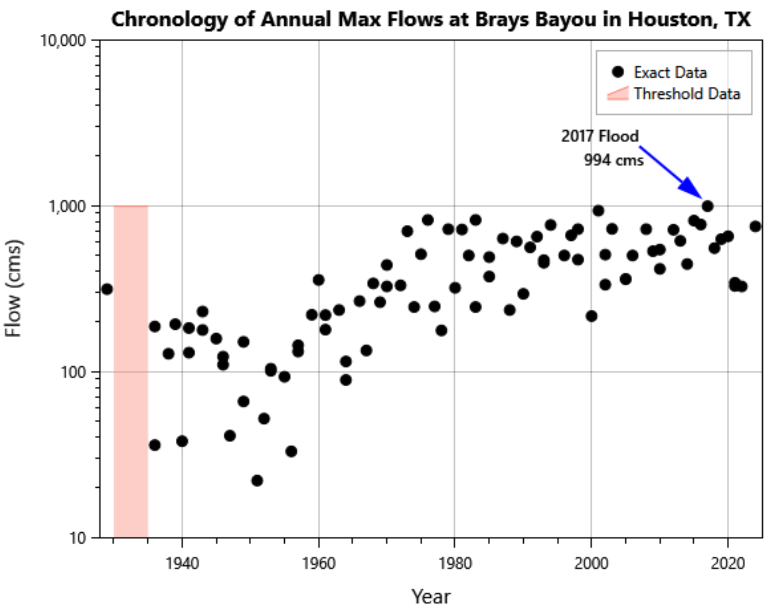
Figure 2.
Autocorrelation function for Brays Bayou at Houston. Persistent positive autocorrelation with slow decay is characteristic of a strong monotonic trend. Dashed lines indicate 95% confidence bounds.
Figure 2.
Autocorrelation function for Brays Bayou at Houston. Persistent positive autocorrelation with slow decay is characteristic of a strong monotonic trend. Dashed lines indicate 95% confidence bounds.
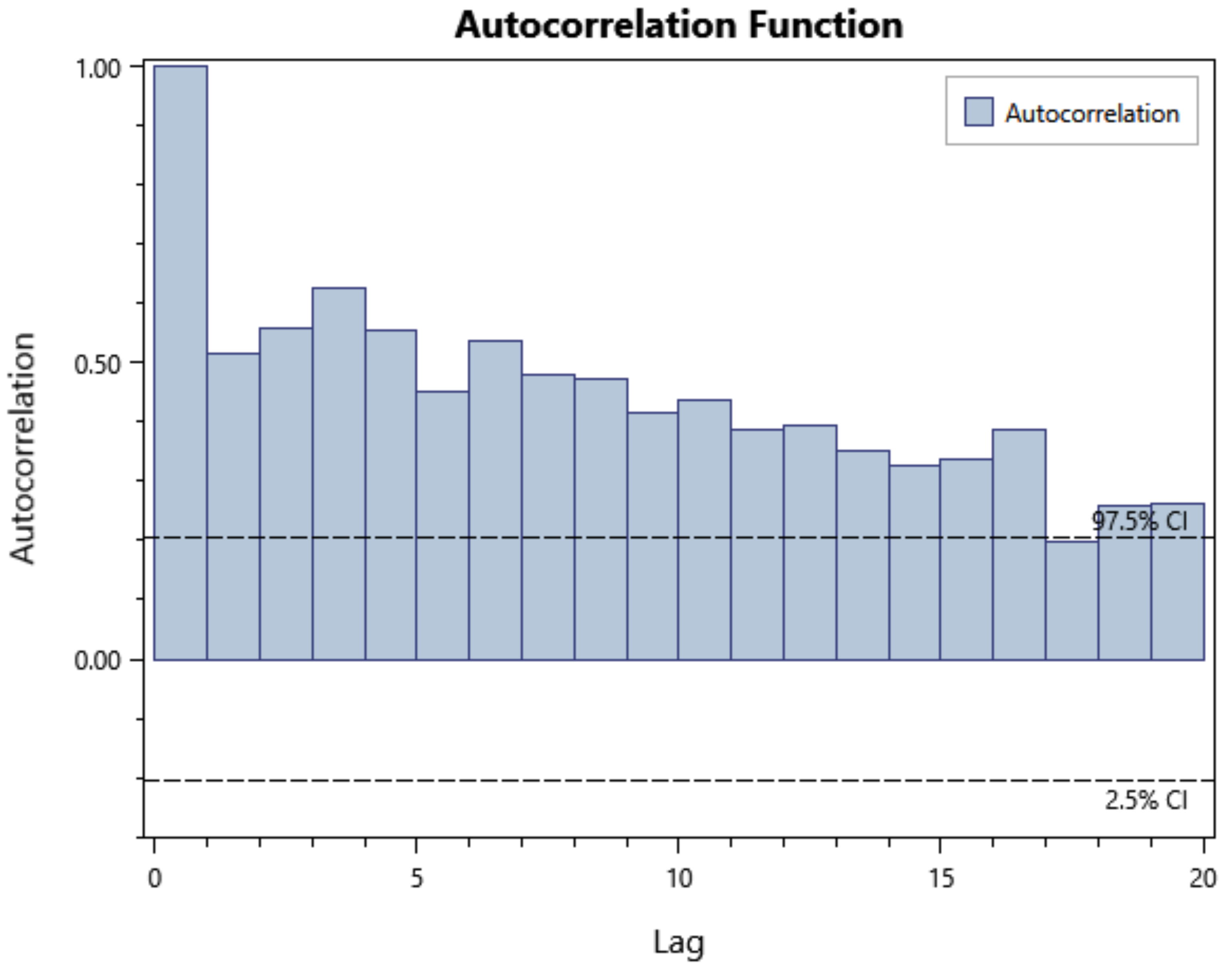
Figure 3.
Comparison of trend model fits for Brays Bayou showing the time-varying 2-year flood distribution: (a) stationary, (b) linear–logistic (–) [DIC = 16.74], (c) logistic–logistic (–) [DIC = 4.95], and (d) step–logistic (–) [selected, DIC = 0]. Dashed lines indicate posterior mean; shaded regions show 90% credible intervals. The selected step–logistic model (d) captures both the regime shift in mean flood magnitude around 1968 and the decreasing variance as urbanization homogenized the watershed’s runoff response.
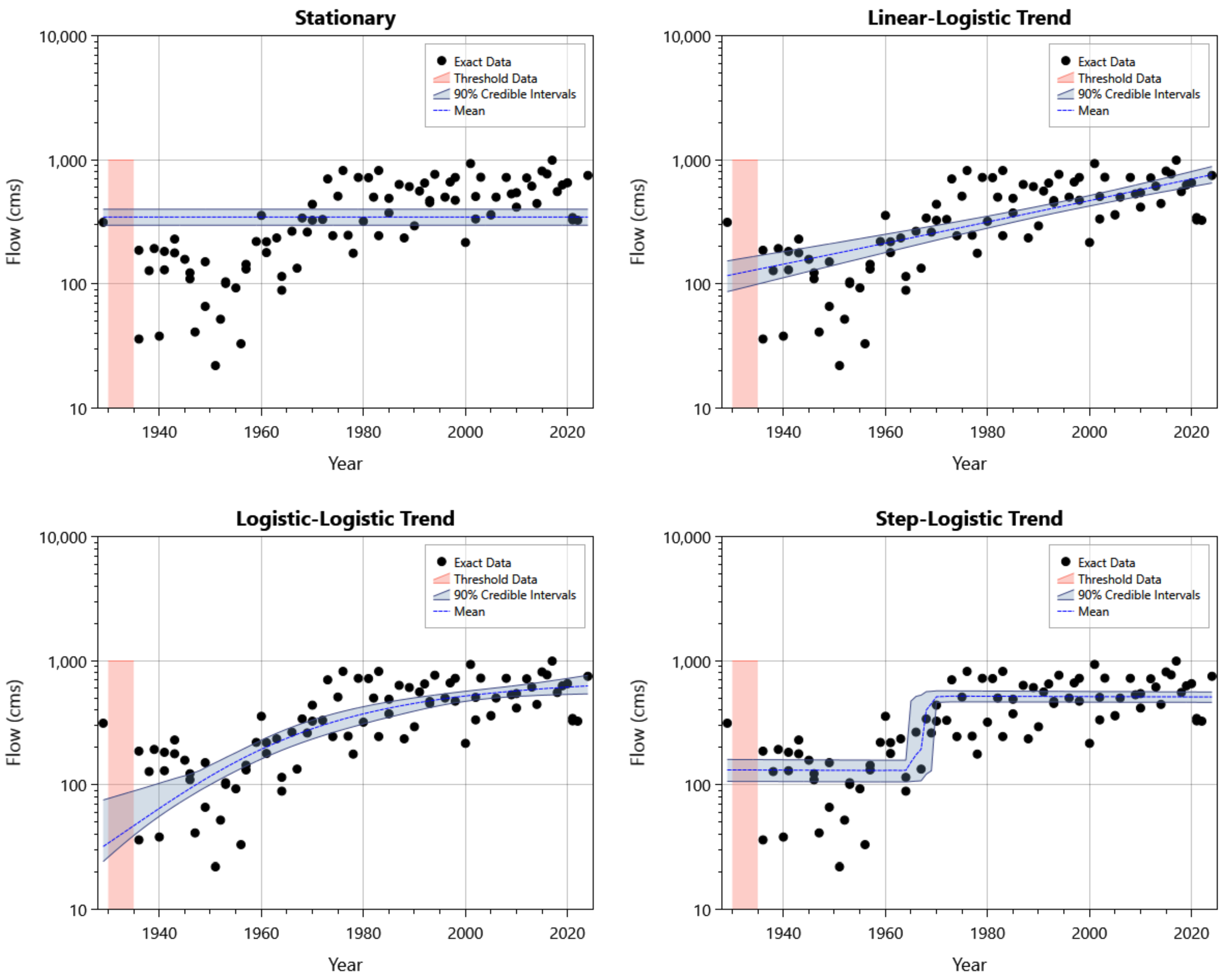
Figure 4.
Flood frequency curves for Brays Bayou at Houston comparing stationary (blue) and nonstationary (red) analyses. Dashed lines represent posterior predictive estimates; shaded regions show 90% credible intervals. The nonstationary curve reflects current watershed conditions (2024). Curves differ substantially for frequent events but converge in the extreme tail due to opposing trends in location and scale parameters. Plotting positions for observed data use the Hirsch-Stedinger formula and implicitly assume stationarity, highlighting the inherent challenge of visualizing nonstationary frequency curves.
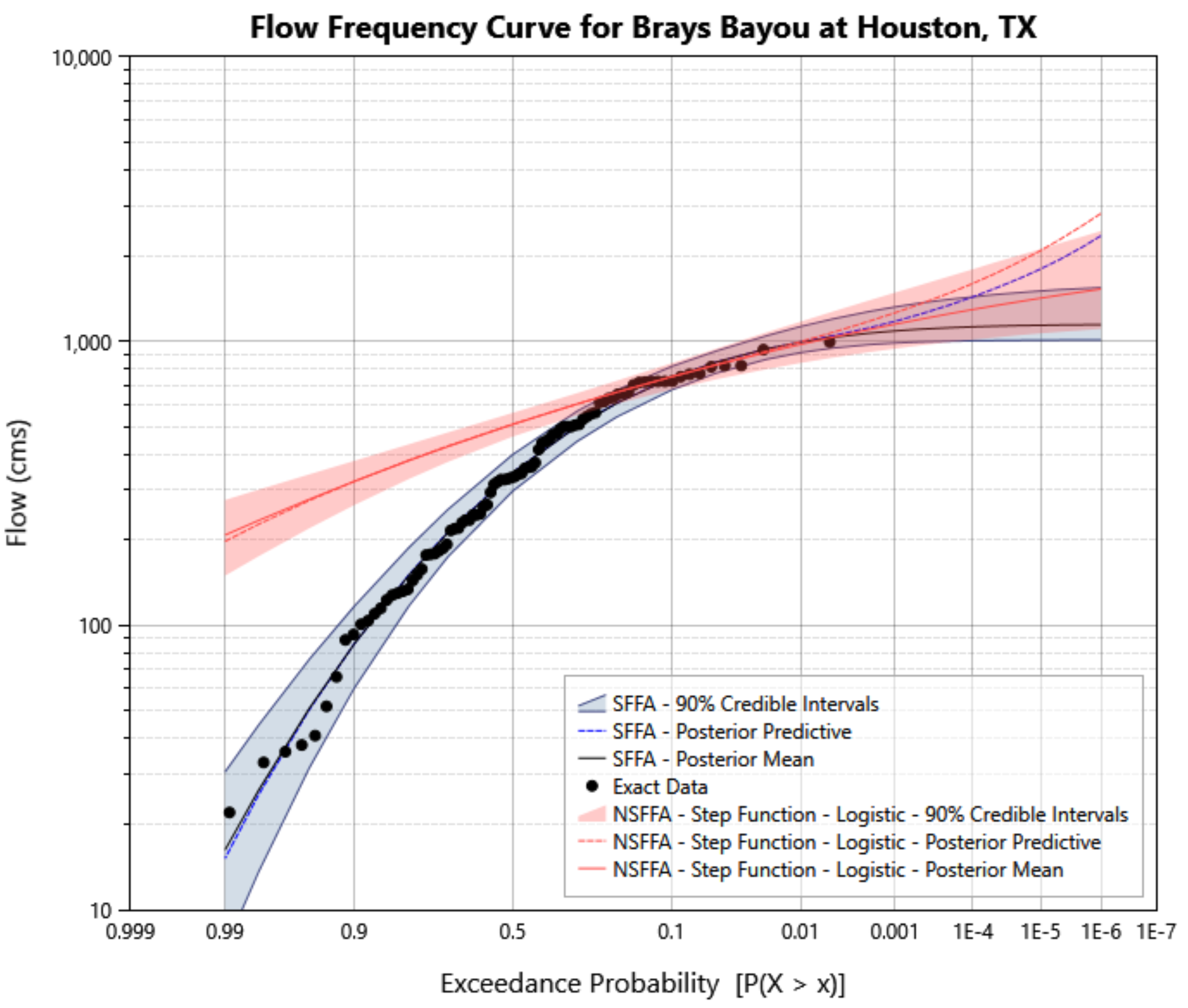
Figure 5.
Chronology of annual maximum 2-day average inflow for O.C. Fisher Reservoir (1853–2021). The historical period 1853–1915 (shaded region) is treated as threshold-censored below the 1936 flood magnitude of 1,150 m3/s. A clear decreasing trend is evident, attributed to brush encroachment and groundwater extraction.
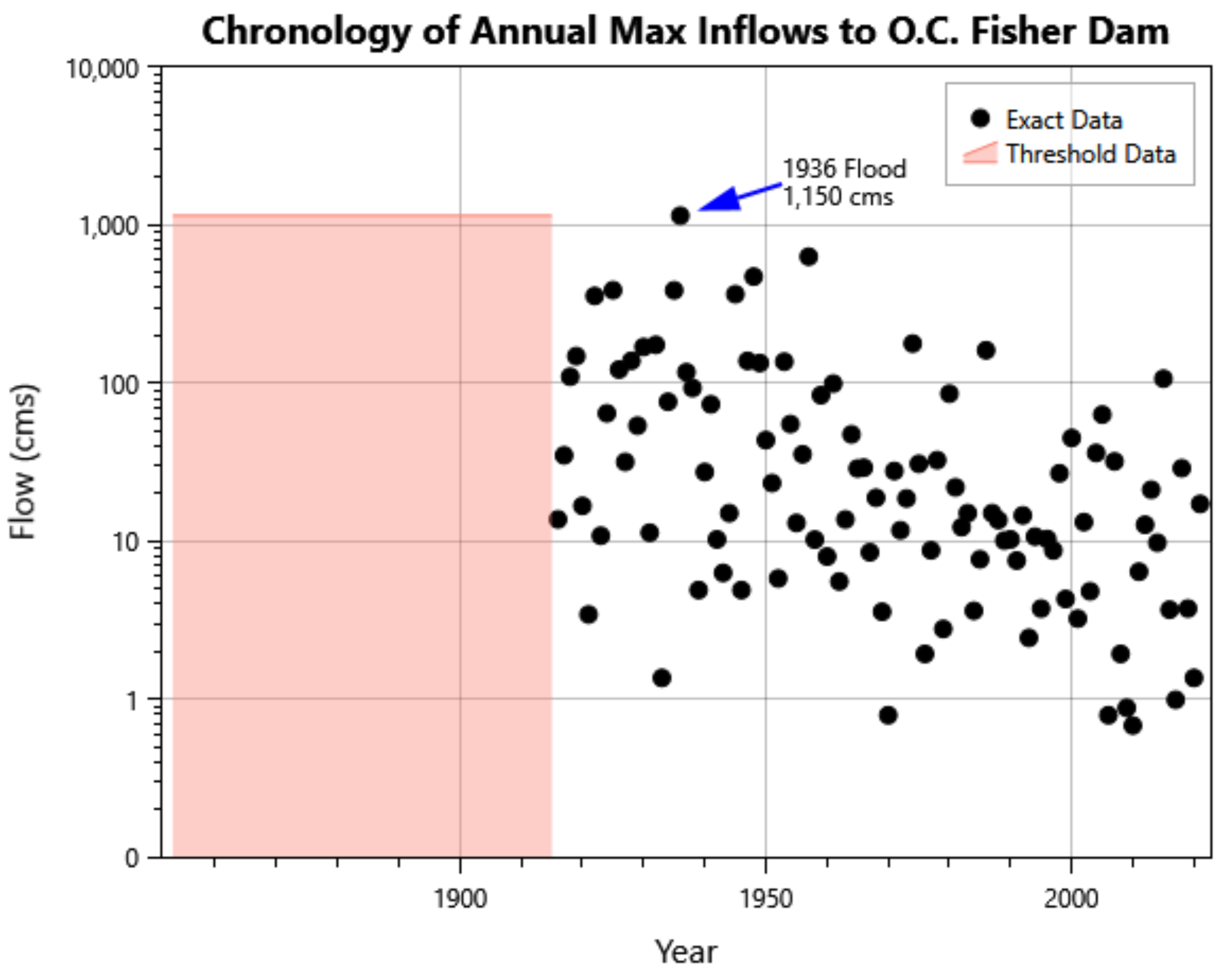
Figure 6.
Autocorrelation function for O.C. Fisher Reservoir. Oscillatory behavior with peaks around lags 9–12 years is consistent with known teleconnection periods (ENSO, PDO); however, the fitted sinusoidal model converged to a period of approximately 50–60 years that does not match these signals, informing selection of the step function model. Dashed lines indicate 95% confidence bounds.
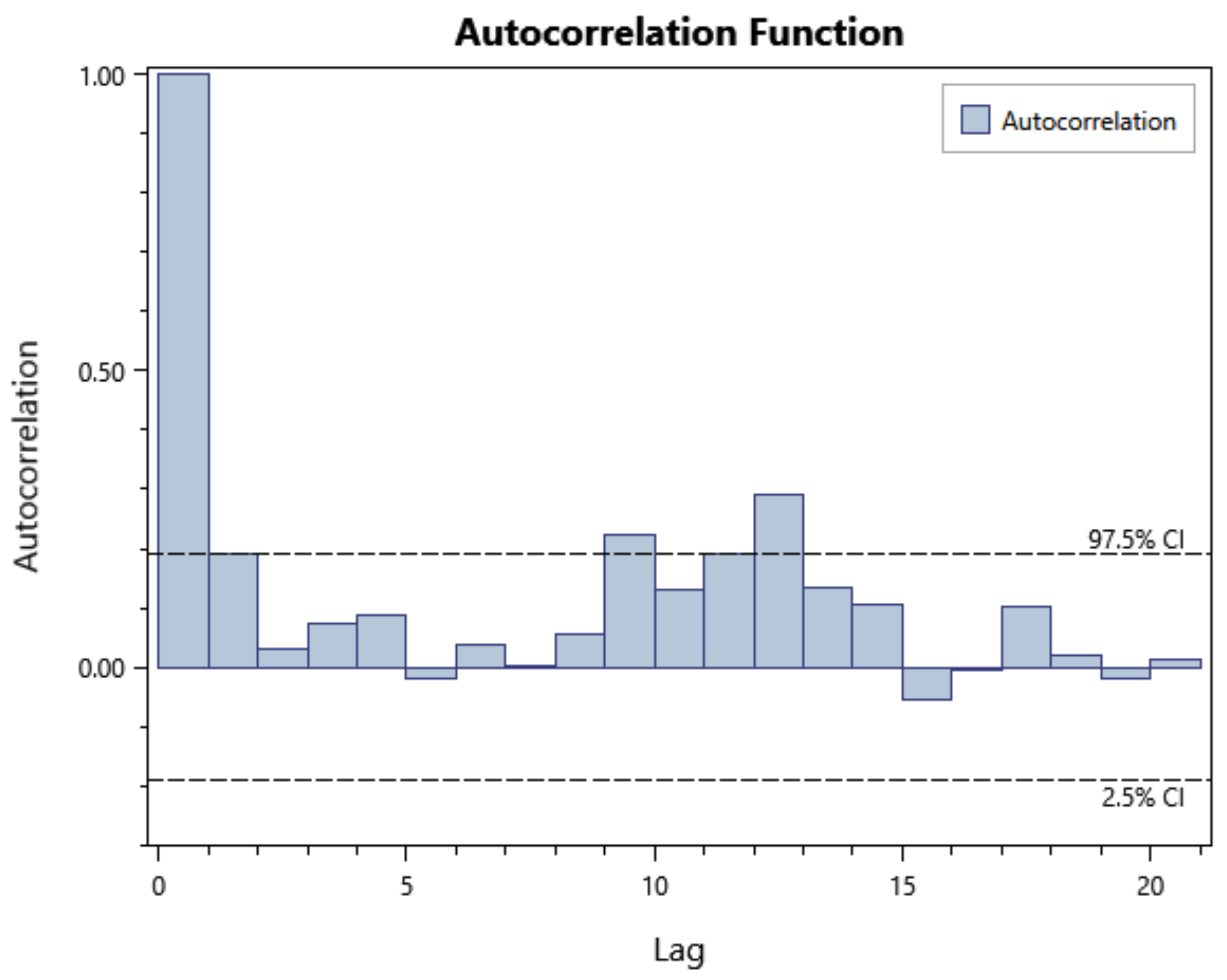
Figure 7.
Comparison of trend model fits for O.C. Fisher Reservoir showing the time-varying 2-year flood distribution: (a) stationary, (b) linear trend, (c) step function, and (d) sinusoidal. Dashed lines indicate posterior mean; shaded regions show 90% credible intervals. Historical threshold-censored period (1853–1915) shown in pink shading. The sinusoidal model (d) achieves the best statistical fit but implies physically implausible cyclic behavior; the step function model (c) was selected based on physical reasoning.
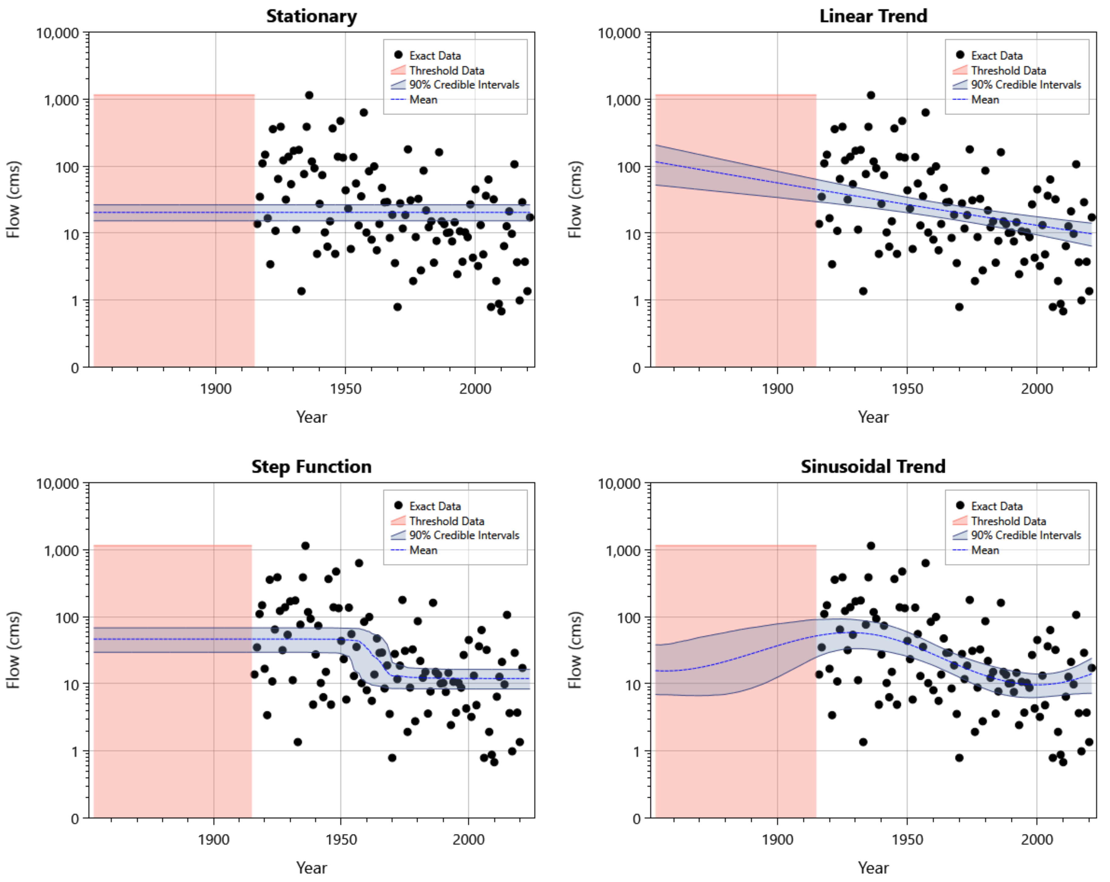
Figure 8.
Flood frequency curves for O.C. Fisher Reservoir comparing stationary (blue) and nonstationary (red) analyses. Dashed lines represent posterior predictive estimates; shaded regions show 90% credible intervals. The nonstationary curve reflects current watershed conditions (2024). The Probable Maximum Flood (PMF) is shown as a horizontal dashed line for dam safety reference. Uniform difference across all return periods reflects the decrease in location parameter only.
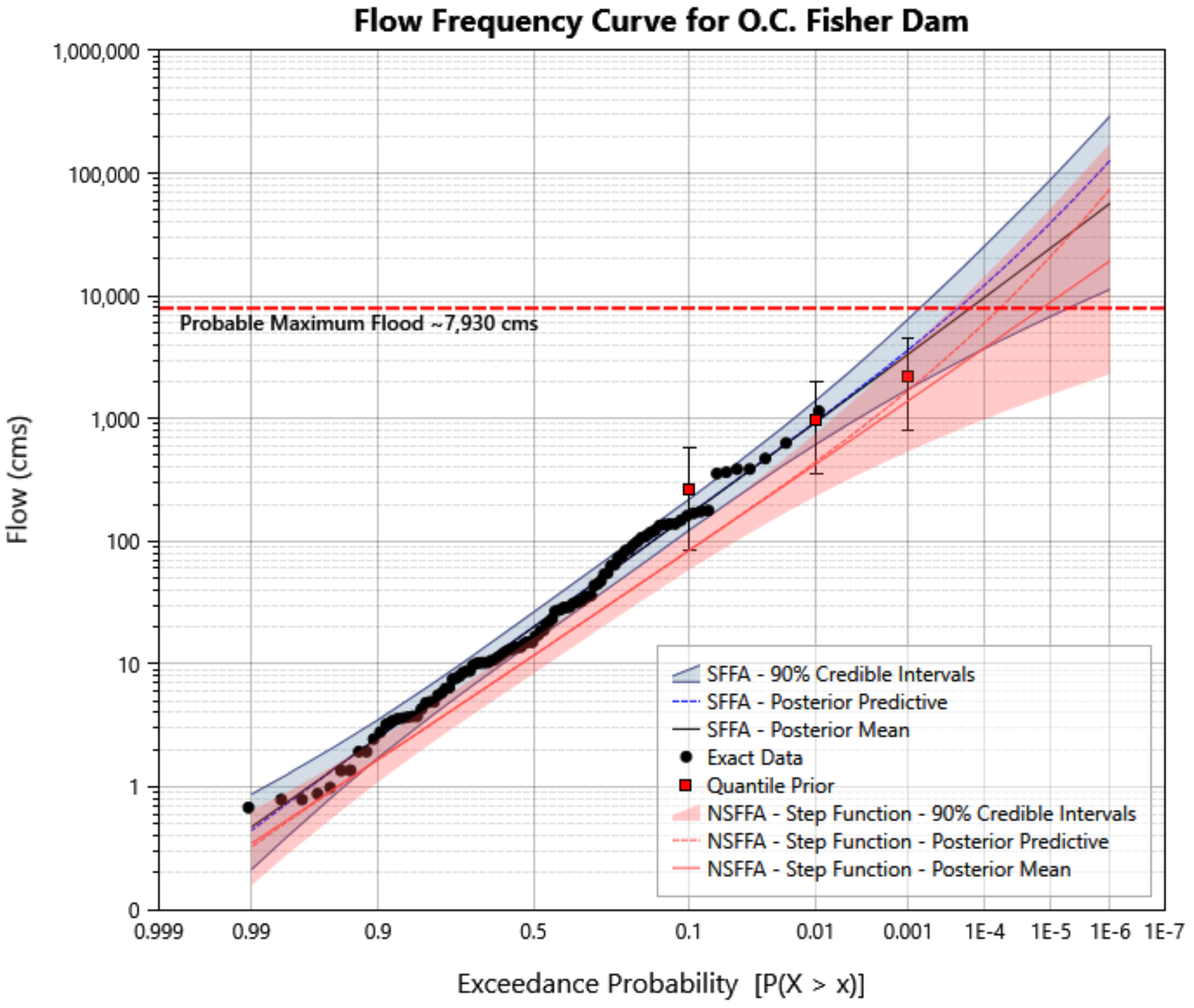
Table 1.
Trend model formulations and applications for urban watersheds.
| Model | Formulation | Use-Case and Hydrologic Example |
|---|---|---|
| Constant | No detectable trend. Rural watershed with no significant land use changes. | |
| Linear | Steady trends in flood magnitude. Increasing flood peaks due to gradual urban expansion [5]. | |
| Exponential | Rapidly decelerating trends. Slowing trend as watershed stabilizes after land use changes. | |
| Logistic | Saturating growth behavior. Urban sprawl drives flood risk upward but plateaus as zoning reaches capacity [6]. | |
| Power | Accelerating trends. Impervious surface growth outpaces population in rapidly urbanizing areas. | |
| Quadratic | Turning points or parabolic behavior. Floods increase then plateau following green infrastructure. | |
| Cubic | Complex evolution with multiple inflection points. A basin affected by sequential changes: deforestation → partial reforestation → late-stage sprawl. | |
| Sinusoidal | Oscillatory behavior. Multidecadal climate cycles influencing rainfall variability [27]. | |
| Step Function | Sudden shifts in flood regime. Significant land cover change in known year. |
Table 3.
Model comparison for Brays Bayou case study.
| Model | k | AIC | BIC | DIC | DIC |
|---|---|---|---|---|---|
| Stationary | 3 | 1233.73 | 1241.23 | 1228.36 | 73.06 |
| Linear () | 4 | 1182.14 | 1192.14 | 1180.76 | 25.45 |
| Logistic () | 4 | 1179.94 | 1189.94 | 1179.23 | 23.93 |
| Step () | 5 | 1177.04 | 1189.54 | 1162.28 | 6.98 |
| Linear–Logistic (–) | 5 | 1168.70 | 1181.20 | 1172.04 | 16.74 |
| Logistic–Logistic (–) | 5 | 1161.46 | 1173.96 | 1160.26 | 4.95 |
| Step–Logistic (–) | 6 | 1165.24 | 1180.24 | 1155.30 | 0.00 |
k = number of parameters. Bold indicates selected model (lowest DIC with identifiable change point).
Table 4.
Flood quantile estimates for Brays Bayou at Houston.
| Stationary | Nonstationary (2024) | |||
|---|---|---|---|---|
| AEP (Return) | Posterior Predictive | 90% CI | Posterior Predictive | 90% CI |
| 0.50 (2-yr) | 346 | [297, 400] | 511 | [462, 560] |
| 0.20 (5-yr) | 607 | [542, 673] | 661 | [603, 727] |
| 0.10 (10-yr) | 744 | [674, 815] | 749 | [675, 836] |
| 0.02 (50-yr) | 940 | [865, 1,046] | 924 | [798, 1,076] |
| 0.01 (100-yr) | 993 | [912, 1,126] | 996 | [838, 1,172] |
AEP = Annual Exceedance Probability; CI = Credible Interval from posterior predictive distribution; Units: m3/s.
Table 6.
Model comparison for O.C. Fisher case study.
| Model | k | AIC | BIC | DIC | DIC |
|---|---|---|---|---|---|
| Stationary | 3 | 1061.42 | 1069.41 | 1051.80 | 24.96 |
| Linear | 4 | 1044.61 | 1055.26 | 1034.06 | 7.22 |
| Step Function | 5 | 1054.21 | 1067.52 | 1029.12 | 2.28 |
| Sinusoidal | 6 | 1044.27 | 1060.25 | 1026.84 | 0.00 |
k = number of parameters. Bold indicates selected model based on physical reasoning despite not having lowest information criteria.
Table 7.
Flood quantile estimates for O.C. Fisher Reservoir.
| Stationary | Nonstationary | |||
|---|---|---|---|---|
| AEP (Return) | Posterior Predictive | 90% CI | Posterior Predictive | 90% CI |
| 0.50 (2-yr) | 20 | [15, 26] | 12 | [8, 16] |
| 0.20 (5-yr) | 80 | [60, 106] | 43 | [30, 60] |
| 0.10 (10-yr) | 165 | [123, 220] | 85 | [59, 120] |
| 0.02 (50-yr) | 598 | [414, 844] | 285 | [166, 458] |
| 0.01 (100-yr) | 947 | [616, 1,405] | 444 | [232, 764] |
AEP = Annual Exceedance Probability; CI = Credible Interval from posterior predictive distribution; Units: m3/s
Disclaimer/Publisher’s Note: The statements, opinions and data contained in all publications are solely those of the individual author(s) and contributor(s) and not of MDPI and/or the editor(s). MDPI and/or the editor(s) disclaim responsibility for any injury to people or property resulting from any ideas, methods, instructions or products referred to in the content. |
© 2026 by the authors. Licensee MDPI, Basel, Switzerland. This article is an open access article distributed under the terms and conditions of the Creative Commons Attribution (CC BY) license (http://creativecommons.org/licenses/by/4.0/).
Copyright: This open access article is published under a Creative Commons CC BY 4.0 license, which permit the free download, distribution, and reuse, provided that the author and preprint are cited in any reuse.


