Entropy in Statistical Mechanics: Back to Boltzmann

Evgenii Rudnyi

doi:10.20944/preprints202602.0005.v1

Submitted:

30 January 2026

Posted:

02 February 2026

You are already at the latest version

Abstract

Statistical entropy introduced in Boltzmann's combinatorial argument played a crucial role in the development of modern physics, yet it is limited to ideal monatomic gases. Statistical mechanics developed by Gibbs is suitable for any system, and this approach yielded important practical results. Unfortunately, the Gibbs statistical entropy remains constant during an irreversible process in the isolated system. This led to the conclusion that entropy is subjective — that entropy of a system is related to ignorance or information gained by an external observer during measurement. At present, arguments for the objectivity of entropy are related to the microcanonical Boltzmann entropy in the system phase space. The advantages and disadvantages of the Boltzmann entropy are discussed. Carnap's principle of physical magnitudes is also considered.

Keywords:

statistical mechanics

;

Boltzmann entropy

;

Gibbs entropy

;

arrow of time

Subject:

Physical Sciences - Thermodynamics

Introduction

Ludwig Boltzmann made important contributions to the development of kinetic theory [1,2]. Statistical entropy and the statistical interpretation of the second law played a major role in the development of physics. For example, Planck’s theory of blackbody thermal radiation, that is, the first discretization of energy, is based on Boltzmann’s ideas [3]. Historian Stephen Brush [4] also emphasizes the importance of discussions on the role of probability in deterministic kinetic theory in the second half of the 19th century on the subsequent arrival of probabilities in quantum mechanics.

Boltzmann’s analysis was limited to a monatomic ideal gas, and the treatment in the general case became possible with the Gibbs ensembles [5]. The Gibbs method led to important results in the development of statistical mechanics. However, formally, the Gibbs statistical entropy in a non-equilibrium process in the isolated system remains constant, and thus there is a contradiction with the second law of thermodynamics. Gibbs himself noted this fact and proposed possible solutions, which were more formally expressed in the Ehrenfests paper in 1911 [6].

The Gibbs statistical entropy gave rise to a subjective interpretation of statistical entropy. This situation was worsened with the arrival of Shannon’s information entropy, which formally resembles the Gibbs statistical entropy. As a result, the interpretation of statistical entropy as a measure of ignorance or as a measure of information about a system from an external observer became rather widespread.

I briefly discuss Rudolf Carnap’s unsuccessful attempt to convince physicists in the mid-1950s in the objectivity of entropy, and then I focus on the modern movement for the objectivity of entropy under the slogan ‘Back to Boltzmann’.

The first section, ‘Boltzmann Statistical Entropy’, briefly examines Boltzmann’s combinatorial argument and its limitations. Due to its clarity, this method is widely used in teaching as an explanation of what entropy is. Unfortunately, its limitations are often not emphasized. This approach is only applicable to a monatomic ideal gas, and hence the properties of a monatomic ideal gas are inadvertently transferred to all systems.

The section ‘Gibbs Statistical Entropy’ then describes the approach by Gibbs and its successes by solving practical problems. The research of mathematicians related to the Gibbs hypothesis of mixing in phase space is presented. The reasons for the arrival of the subjective interpretation of statistical entropy are also outlined.

The section ‘Carnap for Objective Entropy’ discusses Carnap’s arguments based on the principle of physical magnitudes. After that, the main section ‘Back to Boltzmann’ discusses the advantages and disadvantages of the microcanonical Boltzmann entropy. In conclusion, practical research in non-equilibrium statistical mechanics is examined and the problems of statistical entropy are discussed from this viewpoint.

Boltzmann Statistical Entropy

Boltzmann developed the statistical interpretation of entropy in the 1877 paper ‘On the relationship between the second law of mechanical heat theory and probability theory in thermal equilibrium theorems’ [7]:

‘If we apply these to the second law, the quantity that we usually refer to as entropy can be identified with the probability of a respective state. ... The system of bodies we are talking about is in some state at the beginning of time; through the interaction of the bodies this state changes; according to the second law this change must always occur in such a way that the total entropy of all the bodies increases; according to our present interpretation this means nothing other than the probability of the overall state of all these bodies becomes ever greater; the system of bodies always passes from some less probable to some more probable state.’

The state probability, in turn, was associated with the number of microstates corresponding to a macrostate. Let us briefly consider Boltzmann’s method. Boltzmann divided the six-dimensional μ-space of N atoms of the ideal monatomic gas into separate cells by discretizing the values of coordinates and impulses. The state of all atoms in a single cell is considered to be the same as the average values of energy, coordinates, and impulses. The number of cells is equal to p, and it is required that the number of cells is much smaller than the number of atoms N.

N atoms are placed in p cells, and this gives a set of cell occupation numbers: {n₁, n₂, n₃, …, np}; the sum of all occupation numbers is equal to N. This state is referred to as the macrostate; it describes how many molecules have given energy, coordinate, and impulse values in the cells. Now let us enumerate atoms; this is a transition to a microstate. Replacing two atoms in different cells changes the microstate but does not affect the macrostate. Thus, the number of microstates corresponding to a macrostate is determined by the number of possible permutations W(E, V) that depends on energy and volume of the system in question:

W = \frac{N!}{\prod_{i} n_{i}!}

The equilibrium state corresponds to the maximum value of W; the search for a maximum for given values of total energy and volume leads to the Maxwell-Boltzmann energy distribution. All other macrostates have a smaller number of microstates, and hence they are less probable than the equilibrium macrostate.

The number of possible permutations is in turn used in the Boltzmann equation for the entropy of the system, in modern notation:

S = k ln W(E, V)

where k is the Boltzmann constant.

As already mentioned, the statistical interpretation of the second law played a major role in the development of statistical and quantum mechanics, but unfortunately it is often presented as the final answer to the question of what entropy is. This leads to persistent but incorrect metaphors about entropy, such as entropy as the number of permutations and entropy as disorder (see, for example, [8]). Below is a list of limitations for the Boltzmann method.

At present, it is necessary to keep in mind the indistinguishability of atoms. This was already recognized by Gibbs from the requirement of entropy additivity and was further confirmed in quantum statistics. In the quasi-classical approximation, this is achieved by dividing N!, which, however, makes it difficult to interpret the Boltzmann entropy as the ‘number of permutations of microstates’.

The Boltzmann method does not consider kinetics. Non-equilibrium entropies of macrostates are analogous to the entropies of non-equilibrium states in classical thermodynamics. However, in classical thermodynamics time is absent, but statistical mechanics is assumed to be a complete solution also for non-equilibrium thermodynamics. Therefore, the connection between statistical interpretation of entropy and kinetics as well as continuum mechanics remains an open question.

The macrostate in the Boltzmann method is not yet a macrostate in classical thermodynamics. Additional effort is required to find the temperature and pressure fields in the macrostates introduced by Boltzmann. The most important, the Boltzmann method is limited to the ideal monatomic gas and cannot be used in the presence of interactions between atoms and molecules. Thus, this cannot in principle give the universal answer to the question of what entropy is.

Gibbs Statistical Entropy

Gibbs proposed a general framework to consider an arbitrary system with interacting atoms and molecules. Ludwig Boltzmann praised Gibbs’ book; in the lecture ‘On Statistical Mechanics‘ in 1904 the role of Gibbs was emphasized:

‘The merit of having systematized this system, described it in a sizable book and given it a characteristic name belongs to one of the greatest of American scientists, perhaps the greatest as regards pure abstract thought and theoretical research, namely Willard Gibbs, until his recent death professor at Yale College. He called this science statistical mechanics.’

Gibbs introduced an ensemble of systems to visualize the probability density in a multidimensional Γ-space. A deterministic trajectory of a mechanical system is represented as a line, and a single point represents the current state of the system (coordinates and impulses of all particles). The Gibbs ensemble allows for a frequency interpretation of the probability density. In the development of statistical mechanics, it was the Gibbs method that was extended to quantum mechanics, that in turn formally introduced the quasi-classical approximation.

The Gibbs ensemble method in equilibrium statistical mechanics led to the relationship between the Helmholtz energy and the partition function [9,10], making it possible in some cases to compute thermodynamic properties of a substance from molecular constants. Let me note the 2023 paper ‘Ab initio calculation of fluid properties for precision metrology’ [11], in which the accuracy of the results of first-principles calculations of helium properties exceeds that of existing experimental results.

However, in the Gibbs method, the problem of the arrow of time remains. The change in probability density in time is governed by the Liouville equation, which is derived from the Hamilton equations of motion; as a result, the Liouville equation is also symmetric with respect to time. Gibbs introduced the system entropy as the average logarithm of the probability density [5,6]; this is a generalization of the Boltzmann H-function. Below there is the equation for Gibbs entropy in the discrete case:

S = - k \sum_{i} p_{i} (E_{i}) l n p_{i} (E_{i})

This is the sum over all energy levels of the system; the average logarithm of the probability of the system is converted to entropy by multiplying the Boltzmann constant and by changing the sign, like the case of the Boltzmann H-function.

In the equilibrium state, the system obeys the Gibbs energy distribution, and the equation above leads to the correct entropy associated with the partition function. Thus, in equilibrium systems, there are no issues with the Gibbs statistical entropy; actually, this equation is used to derive the relationship between the partition function and the Helmholtz energy of the system.

However, due to the peculiarities of the Liouville equation (the Liouville theorem), when the probability density changes, the average logarithm of the probability density remains constant [5,6]. As a result, the Gibbs statistical entropy remains formally constant during an irreversible process in the isolated system, which contradicts the second law of thermodynamics.

Gibbs understood the limitation of the statistical entropy he introduced. In his book, ideas were proposed as possible solutions: phase volume mixing and the need to change the order of averaging to estimate entropy. These ideas were expressed as equations in the paper ‘The Conceptual Foundations of the Statistical Approach in Mechanics‘ by Ehrenfests in 1911 [6], where the concepts of coarse-grained and fine-grained probability density, as well as coarse-grained and fine-grained Gibbs statistical entropy, were introduced. The coarse-grained Gibbs statistical entropy uses the coarse-grained probability density in the isolated system and thus increases as expected.

In practical work, additional assumptions are used to obtain correct results. For example, in the BBGKY (Bogoliubov-Born-Green-Kirkwood-Yvon) chain of equations, a path was proposed for deriving kinetic equations by introducing time asymmetry at the final stage. Another successful application of non-equilibrium statistical mechanics is related to the development of the linear response theory to assess the transport properties. In this case, time asymmetry was also deliberately introduced during the solution process. An expressive quote from R. Peierls’ lectures on the theory of transport processes quoted from Zubarev’s book is below [12]:

‘In every theoretical study of transport processes, it is necessary to clearly understand where irreversibility is introduced. If it is not introduced, the theory is incorrect. An approach that preserves time-reversal symmetry inevitably leads to zero or infinite values for transport coefficients. If we do not see where irreversibility has been introduced, we do not understand what we are doing.’

At the same time, physicists want to find the arrow of time in statistical mechanics without additional hypotheses. The fundamental laws of physics are time-symmetric, but since these laws are fundamental, a general solution must be found at this level. Additional hypotheses imply that the fundamental laws of physics are incomplete, which is unacceptable to physicists.

Phase Space Mixing

One argument for the arrow of time in the general form is related to Gibbs’ idea of phase space mixing. Mathematicians introduced a formal definition of this process (Hopf, 1937) and found a distinction between mixing and ergodicity (the idea that the time average is equal to the ensemble average). A few theorems were proved, and the ideas of mixing were combined with the development of the formalism of deterministic chaos. Below there are quotes from Mukhin’s dissertation ‘Development of the Concept of Dynamic Chaos in the USSR‘ [13]:

‘Mixing systems formed the basis of Nikolai Sergeevich Krylov’s pioneering work on the foundations of statistical mechanics, a very talented and early deceased student of V. A. Fock. ... According to Krylov, “... the laws of statistics and thermodynamics exist because for statistical systems (which are mixing-type systems), the uniform law of distribution of initial microscopic states within the empirically determined region of phase space ΔГo is valid. ... In this work, the concept of ergodicity is not considered. We reject the acceptance of the ergodic hypothesis. We proceed from the notion of motions of the mixing type. … Such a mixing is due to the fact that in the n-dimensional configuration space, trajectories close at the beginning diverge very quickly, so that their normal distance increases exponentially».’

‘Krylov’s idea is expressed quite clearly. At the heart is the concept of mixing, which can be used to describe the physical process of relaxation — the transition of a system to a stationary state, regardless of its initial state. Since Gibbs, the idea of the need for mixing in statistical mechanics has been repeatedly proposed, but it is probably Krylov who first connected mixing with the local characteristic of motion in such systems — exponential instability.’

Unfortunately, it is impossible to provide a general proof of the existence of mixing for all systems considered in physics, and a simple reference to the large number of particles in the system is insufficient:

‘In physics, it has been common to think that in systems with a large number of degrees of freedom, such as systems of statistical mechanics, the transitive case and mixing are of primary importance, while systems with a small number of degrees of freedom exhibit regular behavior. Kolmogorov notes that this idea appears to be based on a predominant focus on linear systems and a small set of integrable classical problems, and that these ideas have limited significance. Kolmogorov’s key idea is that there is no gap between two types of behavior – regular and complex, irregular – multidimensional systems can demonstrate regular motion, and systems with a small number of degrees of freedom can be chaotic.’

Thus, the use of mixing with deterministic chaos to explain the arrow of time remains at the level of a general hypothesis without complete proof.

From Gibbs Entropy to Subjective Entropy

For many reasons, the Gibbs ensemble method led to the conclusion that entropy is subjective. For example, the Ehrenfests’ explanation with coarse-grained entropy was interpreted as the need for human intervention and thus evidence in favor of the entropy subjectivity. This was further influenced by Shannon’s information theory that appeared in 1948, where the expression for information entropy is like that of the Gibbs statistical entropy.

Also, probabilities in the Gibbs ensemble method began to be interpreted as a measure of ignorance. Kinetic theory was limited to rarefied gases and thus the probabilities could be interpreted as statistics. For example, Maxwell’s velocity distribution represents the statistics of the motion of all atoms. At a given moment in time, the number of atoms moving within a given velocity interval, regardless of their location, makes a histogram. The probability of an atom having a velocity within the range of v±dv is equal to the ratio of the number of atoms with velocities within this interval to the total number of atoms. Thus, the probability for Maxwell’s velocity distribution or the Maxwell-Boltzmann energy distribution has a simple and intuitive frequency interpretation.

In the Gibbs ensemble method, the situation becomes significantly more complex. Let me start with the quote by Gibbs in the introduction to statistical mechanics [5]. Gibbs introduces the transition to an ensemble of systems this way:

‘We may imagine a great number of systems of the same nature, but differing in the configurations and velocities which they have at a given instant, and differing not merely infinitesimally, but it may be so as to embrace every conceivable combination of configuration and velocities. And here we may set the problem, not to follow a particular system through its succession of configurations, but to determine how the whole number of systems will be distributed among the various conceivable configurations and velocities at any required time, when the distribution has been given for some one time.’

In textbooks, systems included in the Gibbs ensemble are called mental or imaginary copies. This provides a visual model and allows us to consider the practical application of formalism after that. The conceptual model of the Gibbs ensemble defines a frequency interpretation of the probability density distribution in phase space and thus supports objectivity of probabilities (frequency interpretation) employed to find connections between the micro- and macrosystems.

However, a transfer from such a view to the real world raises serious difficulties. This is particularly controversial among philosophers of physics, who attempt to build a bridge from statistical mechanics to the worldview. A good example is a recent article by philosophers on this topic with the expressive title ‘Can somebody please say what Gibbsian statistical mechanics says?’ [14].

The main point is that during transfer to the world, the Gibbs ensemble must correspond to a single system under study, since only in this case can we proceed to consider real experiments. As a result, an interpretation of probability for a single system must be found. In this case, it is difficult to preserve probability as an objective quantity, and this has provided additional arguments in favor of interpreting probability as a measure of ignorance. Thus, entropy and probabilities in statistical mechanics often are associated with human ignorance of the real state of affairs at the microscopic level.

Carnap for Objective Entropy

Rudolf Carnap wrote a book on entropy between 1952 and 1954 during his stay at the Institute for Advanced Study in Princeton, but the book was published just in 1977 posthumously [15,16]. Carnap’s interest in entropy in statistical mechanics was related to his work on inductive logic. He believed that interpretation of probability within the framework of logic could lead to a partial verification approach. At present, the similarity between Carnap’s ideas and the later development of Bayesian statistical inference is emphasized.

Carnap saw the similarity of mathematical formalism in the statistical interpretation of thermodynamic entropy and in solution of inductive logic problems within the framework of partial verification. Carnap compares the task of distributing gas molecules among the cells of μ-space in the Boltzmann method with the task of object classification into categories that arises in inductive logic. The number of possible arrangements of objects into categories coincides with the number of distributions of gas molecules among the cells, resulting in two entropies that formally appear to be the same.

At the same time, Carnap emphasized the fundamental difference between these tasks; he believed that the similarity of mathematical formalism does not lead to the identical meaning in both tasks, therefore, to the same meaning of both entropies. In his autobiography written in 1963, Carnap described the atmosphere of that time as follows:

‘I had some talks separately with John von Neumann, Wolfgang Pauli, and some specialists in statistical mechanics on some questions of theoretical physics with which I was concerned. I certainly learned very much from these conversations; but for my problems in the logical and methodological analysis of physics, I gained less help than I had hoped for. … My main object was not the physical concept, but the use of the abstract concept for the purposes of inductive logic. Nevertheless, I also examined the nature of the physical concept of entropy in its classical statistical form, as developed by Boltzmann and Gibbs, and I arrived at certain objections against the customary definitions, not from a factual-experimental, but from a logical point of view. It seemed to me that the customary way in which the statistical concept of entropy is defined or interpreted makes it, perhaps against the intention of the physicists, a purely logical instead of physical concept; if so, it can no longer be, as it was intended to be, a counterpart to the classical macro-concept of entropy introduced by Clausius, which is obviously a physical and not a logical concept. The same objection holds in my opinion against the recent view that entropy may be regarded as identical with the negative amount of information. I had expected that in the conversations with the physicists on these problems, we would reach, if not an agreement, then at least a clear mutual understanding. In this, however, we did not succeed, in spite of our serious efforts, chiefly, it seemed, because of great differences in point of view and in language.’

Carnap assumes the objectivity of entropy in classical thermodynamics:

‘The concept of entropy in thermodynamics (S_th) had the same general character as the other concepts in the same field, e.g., temperature, heat, energy, pressure, etc. It served, just like these other concepts, for the quantitative characterization of some objective property of a state of a physical system, say, the gas g in the container in the laboratory at the time t.’

This in turn implies the objectivity of entropy in statistical mechanics, and Carnap introduced the principle of physical magnitudes, which states that physical descriptions of a quantity at the micro and macro levels should lead to the same results within the experimental error.

The main difference between two entropies, in statistical mechanics and inductive inference, is related to microstate entropy. In the classification problem, for a specific microstate all uncertainties disappear, and the information entropy becomes zero. Carnap referred to this solution as the second method for determining microstate entropy (Method II). Carnap believed that this solution was suitable for logical problems, as there was no contradiction between the non-zero entropy of the macrostate and the zero entropy of the microstate.

However, this approach is inconsistent with the principle of physical magnitudes and therefore Carnap believed that such a solution could not be used in statistical mechanics. The microstate belongs to a physical system, and therefore its properties are as objective as the properties of the macrostate. According to Carnap, experimental measurements correspond to the trajectory of a single system over time, and averaging over phase space is merely a technical method for finding time averages.

A microstate specifies a certain trajectory in time, so the physical properties of the system under study must also relate to a single microstate. Hence, Carnap concluded that the microstate entropy must be equal to the macrostate entropy; otherwise, it becomes unclear how a macrostate can have a non-zero entropy as the system moves along its trajectory. Carnap refers to this solution as the first method for calculating microstate entropy (method I).

At the end, Carnap’s main conclusion was that the first method of calculating the microstate entropy should be used in statistical mechanics as a branch of theoretical physics, and the second method should only be considered when solving epistemological problems. This led to serious disagreements with physicists. John von Neumann and Wolfgang Pauli believed that the second method was correct for entropy in statistical mechanics (the entropy of a microstate is equal to zero), and that Carnap’s book was therefore undesirable. Pauli wrote after reviewing Carnap’s draft as follows:

‘Dear Mr. Carnap! I have studied your manuscript a bit; however I must unfortunately report that I am quite opposed to the position you take. Rather, I would throughout take as physically most transparent what you call “Method II”. In this connection I am not all influenced by recent information theory (…) Since I am indeed concerned that the confusion in the area of foundations of statistical mechanics not grow further (and I fear very much that a publication of your work in this present form would have this effect).’

Similar arguments were made by von Neumann. As a result, Carnap abandoned the idea of publishing the book.

Back to Boltzmann

Technically, statistical Gibbs entropy is associated with the integral over the entire phase space, while the Boltzmann entropy is associated with the number of microstates. This gives Boltzmann entropy a clearer physical meaning, since in this interpretation, probabilities appear only after the introduction of entropy. This was already noted in the Ehrenfests’ paper [6]:

‘it is also clear that Gibbs’s measure of entropy is unable to replace Boltzmann’s measure of entropy in the treatment of irreversible phenomena in isolated systems, since it indiscriminately includes the initial nonequilibrium states with the final equilibrium.’

This line is advanced by a few physicists using the Boltzmann method in the microcanonical ensemble. Thus, the microcanonical Boltzmann entropy becomes the main foundation for the arrow of time, and a service role is left for the Gibbs statistical entropy. I quote from the conclusion of the paper by theoretical physicists ‘Gibbs and Boltzmann entropy in classical and quantum mechanics‘ [17]:

‘The Gibbs entropy is an efficient tool for computing entropy values in thermal equilibrium when applied to the Gibbsian equilibrium ensembles, but the fundamental definition of entropy is the Boltzmann entropy. We have discussed the status of the two notions of entropy and of the corresponding two notions of thermal equilibrium, the “ensemblist” and the “individualist” view. Gibbs’s ensembles are very useful, in particular as they allow the efficient computation of thermodynamic functions, but their role can only be understood in Boltzmann’s individualist framework.’

To a greater extent, this point of view is dramatized in the works of philosophers of physics, who search for an ideal foundation for statistical mechanics. Below there are quotes from the paper ‘Philosophy of Statistical Mechanics‘ [18] (BSM and GSM refer to Boltzmann and Gibbs statistical mechanics, respectively):

‘philosophical discussions in statistical mechanics face an immediate difficulty because unlike other theories, statistical mechanics has not yet found a generally accepted theoretical framework or a canonical formalism.’

‘Finally, there is no way around recognising that BSM is mostly used in foundational debates, but it is GSM that is the practitioner’s workhorse. When physicists have to carry out calculations and solve problems, they usually turn to GSM which offers user-friendly strategies that are absent in BSM. So either BSM has to be extended with practical prescriptions, or it has to be connected to GSM so that it can benefit from its computational methods.’

Let us consider the basic idea of the microcanonical Boltzmann entropy (below just Boltzmann entropy) using a figure from the website universe-review.ca - Thermodynamics [19] and quotes from Penrose’s book [20]:

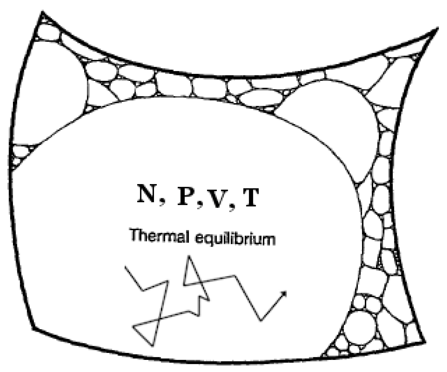
In the figure, the surface of the phase space with a given energy is shown. This surface is of very high dimensionality, but a simple plane is used for simplicity. Each cell represents a macrostate with many microstates, and the area of the cell is proportional to the number of microstates. The largest cell represents the equilibrium state with uniform temperature, while the other cells represent non-equilibrium states. The difference with the Boltzmann equation is the transition from μ-space to Γ-space and the replacement of the number of permutations with the area of the surface in Γ-space. The transition to Γ-space allows us to speak about the universality of such an explanation.

Below there are quotes from Roger Penrose’s book ‘Fashion, Faith, and Fantasy in the New Physics of the Universe‘ [20], which explain the idea shown in the figure in more detail:

‘What, then, is this “measure of entropy”? Roughly speaking, what we do is to count all the different possible submicroscopic states that could form a particular macroscopic state, and the number of these states N is a measure of the entropy of the macroscopic state. The larger N is, the greater the entropy.’

‘This is, indeed, essentially the famous definition of entropy given by the great Austrian physicist Ludwig Boltzmann in 1872.’

‘it is best that we return to the notion of phase space … the phase space P, of some physical system, is a conceptual space, normally of a very large number of dimensions, each of whose points represents a complete description of the submicroscopic state of the (say, classical) physical system being considered.’

‘Now, in order to define the entropy, we need to collect together - into a single region called a coarse-grained region - all those points in P which are considered to have the same values for their macroscopic parameters. In this way, the whole of P will be divided into such coarse-graining regions. … Thus, the phase space P will be divided up into these regions, and we can think of the volume V of such a region as providing a measure of the number different ways that different submicroscopic states can go to make up the particular macroscopic state defined by its coarse-graining region.’

It is important to note that the picture above is not scaled correctly, and the areas of the non-equilibrium states have been exaggerated for clarity. In the equilibrium microcanonical distribution, the statistical weight corresponds to the entire area in the figure, including the non-equilibrium states. This means that the equal a priori probability principle includes all states, both equilibrium and non-equilibrium, and in turn it shows that the area corresponding to the equilibrium macrostate cell is significantly larger than the areas of the non-equilibrium state cells; the latter would be almost invisible on a proper scale.

Macrostate Entropy

The macrostate entropy in the new approach is related to the statistical weight of a single cell W_v in the Γ-space:

S = k ln W_v

The statistical weight of the equilibrium state using W_v is almost equal to the statistical weight using the entire area, so the entropy of the equilibrium macrostate is indistinguishable from the entropy in the equilibrium microcanonical ensemble. At the same time, this approach defines the entropies of non-equilibrium states, which can be used now as a foundation for the arrow of time. Penrose gives the final conclusion as follows:

‘In order to see how this helps in our understanding of the 2nd Law, it is important to appreciate how stupendously different in size the various coarse-graining regions are likely to be, at least in the kind of situation that is normally encountered in practice. The logarithm in Boltzmann’s formula, together with the smallness of k in commonplace terms, tends to disguise the vastness of these volume differences, so that it is easy to overlook the fact that tiny entropy differences actually correspond to absolutely enormous differences in coarse-graining volumes. … Since the (vastly) larger volume corresponds to an (albeit usually only slightly) larger entropy, we see, in general rough terms why the expression for the entropy increases unstoppably over time. This is exactly what we would expect according to the second law.’

Proponents of the new approach argue that the connection of microstates with macrostates excludes subjectivity in the entropy of non-equilibrium states. In parallel, the concept of typicality (typical behavior) is introduced, and it is considered a solution to the Loschmidt and Zermelo paradoxes. For example, the figure above shows that the reversal of velocities for the absolute majority of microstates in the equilibrium state leaves the trajectory of the system in this cell. The direction of the trajectory plays a role only for a negligible number of microstates that are at the boundary of the macrostate; in this sense, the trajectories in the equilibrium state represent the typical behavior of the system.

The figure above also allows us to better understand Carnap’s logic related to the entropy of a microstate. A macrostate corresponds to a system under study, and the macrostate has entropy. On the other hand, the macrostate under study belongs to a specific trajectory of the system, which is a sequence of microstates that belong to the solution of the Hamilton equation of motion. Carnap’s principle of physical magnitudes requires that the entropy in both cases be consistent within the experimental errors; this requires the presence of entropy of the system for a specific trajectory of motion.

In this explanation, which is presented more formally in [17] (see also references to other works), the entropy measure is indeed more objective. Entropy is linked to the properties of the Γ-space, and probabilities are considered after the entropy has been already defined. At the same time, it remains unclear whether this qualitative idea can be translated into the quantitative level. The main difficulty is related to the question of what is a macrostate and how to determine whether a microstate belongs to a given macrostate. The problem of Boltzmann’s original statistical interpretation also remains: the proposed solution cannot be used to consider kinetics and transport equations of continuum mechanics. These issues are considered in the next two sections.

Non-Equilibrium Macrostates and Microstates

To find the connection between macrostate and microstates, Boltzmann used the discretization of cells by the values of coordinates and momenta in μ-space. However, this is impossible in Γ-space. Moreover, as already noted, even in the original Boltzmann method we do not obtain a macrostate in classical thermodynamics. Carnap’s principle of physical magnitudes is specifically designed to the comparison of the macrostate in continuum mechanics with the description in statistical mechanics, since it primarily concerns the interpretation of experiments conducted in continuum mechanics. This is the main problem with the modified Boltzmann equation for the entropy of non-equilibrium states. The equation expresses an idea, but it remains unclear how it could be possible to implement it.

The general idea in [17] is to introduce the properties of a macrostate, and then to enumerate the microstates. For each microstate, macroscopic properties should be evaluated, and this way microstates could be assigned to macrostates. Of course, this procedure is not feasible in practice, but it is assumed that it is possible in principle. In his book Penrose immediately moves on to the universe and the problem of the past hypothesis, which addresses the origin of the low-entropy state in the Big Bang. I limit myself to a more prosaic example of the candle combustion — whether such an idea is possible even in principle.

Let us start with a non-equilibrium state in continuum mechanics, which is characterized by fields of temperature, pressure, and concentrations. The goal is then to determine the necessary fields from a given microstate to compare it with one of the macrostates in continuum mechanics. I believe that this task is unsolvable. Let us consider this issue with the temperature field as an example. We need to convert the coordinates and impulses of all particles in each microstate into a temperature field. In kinetic theory, there is the relationship between temperature and the average kinetic energy of atoms, but this equation is only valid for systems in equilibrium. A more correct way for temperature in statistical mechanics is associated with the achievement of the Maxwell-Boltzmann distribution and with the identification of thermodynamic temperature with the parameter of the Maxwell-Boltzmann distribution.

Hence, the correct way to find the temperature field for a microstate is to introduce a local Maxwell-Boltzmann distribution and identify the local temperature with the parameter of this distribution; this is analogous to the principle of local equilibrium. It remains unclear how this task can be practically accomplished for a given microstate, since at the microstate level a much richer choice of non-equilibrium states appears compared to those in continuum mechanics.

Relaxation time is needed for the energy to be redistributed among different degrees of freedom, and therefore there are macrostates in which there are Maxwell-Boltzmann distributions with different values of the temperature for different degrees of freedom. In these macrostates, the translational, rotational, and vibrational temperatures differ from each other. Statistical mechanics has demonstrated the possibility of new states that were not even imaginable in continuum mechanics.

Other non-equilibrium macrostates are associated with the case where local equilibrium is not reached for all degrees of freedom — the case of non-equilibrium temperature or absence of temperature. Thus, there are macrostates for which relaxation is needed to establish the local Maxwell-Boltzmann distribution. The concept of entropy in such states is beyond the entropy of classical and non-equilibrium thermodynamics, although from experience it is expected that the relaxation processes are rather fast.

The question is as to whether in the microcanonical Boltzmann method one can unambiguously determine to which macrostate a given microstate belongs. Such a postulate forms a basis for the Boltzmann method, but it remains unclear whether this problem could be solved even in principle.

Entropy of Non-Equilibrium States and Kinetics

In the new Boltzmann method, the same problem remains as in the original Boltzmann method. Macrostates are ranked according to their entropy value, as in classical thermodynamics, but time is completely absent.

The absence of time is a distinctive feature of classical thermodynamics. It is possible to predict the direction of a spontaneous process, but it is impossible to say how quickly the process occurs. During the development of thermodynamics and continuum mechanics, this served as a distinction between thermodynamics and transport processes in continuum mechanics (see, for example, [21]). The Clausius inequality belonged to classical thermodynamics, while the question of the process time belonged to kinetics and continuum mechanics. Statistical mechanics, on the other hand, contains time and it should provide an explanation for all processes, including the transport equations of continuum mechanics. The absence of time in the modified Boltzmann method limits the scope of applications of statistical mechanics.

Discussing the typical behavior of a system without considering the actual kinetics is insufficient. Let us take a candle in an air atmosphere in the isolated system. The final global equilibrium state is related to the combustion products, but the combustion does not start on its own. Therefore, a candle in an air atmosphere is also an example of typical behavior. In this case, statistical interpretation of entropy does not explain why the system does not spontaneously move from a state with lower entropy to a state with higher entropy.

On the other hand, explicit inclusion of time is necessary when considering the process of candle combustion. This process continues for a significant amount of time and can also be considered a typical behavior. Candle combustion is kind of a quasi-stationary process, as new reactants are continuously added to the reaction, but the flame remains in a relatively stable state. To achieve such a state, specific rates must be maintained. It is unclear how the modified Boltzmann equation could be useful in this case.

Discussion

Let us return to the Gibbs method in non-equilibrium statistical mechanics. The problem with the Gibbs statistical entropy is related to the Liouville theorem, according to which the Gibbs statistical entropy remains constant in an irreversible process in the isolated system. However, these are general equations that cannot be solved. This is just a short form of extremely long mathematical equations. This is only sufficient for proving mathematical theorems, but the results cannot be used in practice to consider specific cases.

The way to practical problems in non-equilibrium statistical mechanics is based on a hierarchy of approximations. Since the goal is to deal with kinetic experiments, such as relaxation processes, the priority belongs to kinetics and not to the entropy of non-equilibrium states. As a result, the Liouville theorem does not hinder the use of non-equilibrium statistical mechanics for practical applications.

Let me take the book by Zubarev, Morozov and Röpke ‘Statistical Mechanics of Nonequilibrium Processes‘ as an example. The authors discuss the problem of Gibbs entropy and suggest possible solutions related to the order of averaging. However, the coarse-graining and fine-graining Gibbs entropies are not used as a solution to practical problems.

The non-equilibrium states beyond the scope of continuum mechanics are treated by means of different characteristic times; as a result, there are different approaches to kinetics at different stages. The book deals with simplified descriptions of non-equilibrium systems, and there are three different regimes with different characteristic times: dynamic, kinetic, and hydrodynamic. First, there is fast relaxation kinetics followed by a transition to a regime close to the Navier-Stokes equations. The entropy in the book is considered only after the kinetic equations have been derived.

For practical problems, it is necessary to find probability distributions that are relevant to the system in question. In the book, the formalism of the non-equilibrium statistical operator is developed. There are also other methods for finding relevant probability distributions, such as the Zwanzig-Mori projection operator method. In general, physicists understand the specifics of the required solutions, and there are no particular problems with the Gibbs method. Because of the approximations employed to find kinetic equations, the entropy of the system increases as expected.

Now let us recall the original problem. The fundamental equations of classical and quantum mechanics are time symmetric. However, in the isolated macroscopic system, equilibrium is established, and therefore the behavior of the isolated system is asymmetric in time. In practical applications of statistical mechanics, additional assumptions are always introduced in one way or another to describe such system behavior.

The goal of the new Boltzmann method is to find foundations for the arrow of time in the general case without considering practical applications. It must be admitted that at the qualitative level, this approach provides a good visual picture of what is happening. However, there is no clear way to move from a qualitative discussion of the arrow of time to practical applications. In this sense, there is a gap between this explanation and practical work in non-equilibrium statistical mechanics; it’s unclear how this gap could be bridged.

In any case, before moving on to cosmology and the past hypothesis, it would be useful to discuss the application of the Boltzmann method to candle combustion. Since Boltzmann’s time, the search for the foundation of statistical mechanics has traditionally been associated with the task of reducing classical thermodynamics to statistical mechanics. However, classical thermodynamics does not explicitly contain time and the Clausius inequality is a bridge between classical thermodynamics and continuum mechanics [21].

Time is explicit in the equations of continuum mechanics, and these equations are time asymmetric. For example, it is now quite possible to compute candle combustion with numerical methods. Therefore, it would be more reasonable to search for the arrow of time in statistical mechanics by exploring the possibility of deriving time-asymmetric equations of continuum mechanics. In other words, the main question should be whether continuum mechanics could be reduced to statistical mechanics.

References

Cercignani, C. Ludwig Boltzmann: the man who trusted atoms; 1998. [Google Scholar]
Uffink, J. Boltzmann’s Work in Statistical Physics; Zalta, Edward N., Ed.; The Stanford Encyclopedia of Philosophy. First published 2004; substantive revision 2014.
M. J. Klein, Max Planck and the beginnings of the quantum theory. Archive for History of Exact Sciences 1962, 1, 459–479.
Brush, S. The Kind of Motion We Call Heat; 1976. [Google Scholar]
Gibbs, J. W. Elementary Principles in Statistical Mechanics: Developed with Especial Reference to the Rational Foundation of Thermodynamics; 1902. [Google Scholar]
Ehrenfest, P.; Ehrenfest, T. The Conceptual Foundations of the Statistical Approach in Mechanics (1911); 1959. [Google Scholar]
L. Boltzmann, Wissenschaftliche Abhandlungen, Vol. I, II, and III, 1909. Über die beziehung dem zweiten Haubtsatze der mechanischen Wärmetheorie und der Wahrscheinlichkeitsrechnung respektive den Sätzen über das Wärmegleichgewicht. 1877, v. II, paper 42, 164–223.
Rudnyi, E. Erwin Schrödinger and Negative Entropy; 2025; preprint. [Google Scholar] [CrossRef]
Atkins, P.; de Paula, J. Atkins’ Physical Chemistry; 2002. [Google Scholar]
Ya, A. Borshchevsky, Physical Chemistry. In Statistical Thermodynamics; 2023; Volume 2. (In Russian) [Google Scholar]
Garberoglio, G.; Gaiser, C.; Gavioso, R. M.; et al. Ab initio calculation of fluid properties for precision metrology. Journal of Physical and Chemical Reference Data 2023, 52(no. 3). [Google Scholar] [CrossRef]
Zubarev, D. N.; Morozov, V.; Röpke, G. Statistical Mechanics of Nonequilibrium Processes; 1996. [Google Scholar]
Mukhin, R. R. Development of the Concept of Dynamic Chaos in the USSR. In 1950-1980s; (in Russian). 2010. [Google Scholar]
Frigg, R.; Werndl, C. Can somebody please say what Gibbsian statistical mechanics says? The British Journal for the Philosophy of Science 2021, 72:1, 105–129. [Google Scholar] [CrossRef]
Carnap, R. Two essays on entropy; Univ of California Press, 1977. [Google Scholar]
J. Anta Pulido, Historical and Conceptual Foundations of Information Physics. PhD Thesis, 2021.
Goldstein, S.; Lebowitz, J. L.; Tumulka, R.; Zanghì, N. Gibbs and Boltzmann entropy in classical and quantum mechanics. Statistical mechanics and scientific explanation: Determinism, indeterminism and laws of nature 2020, 519–581. [Google Scholar]
Frigg, R.; Werndl, C. Philosophy of Statistical Mechanics. In The Stanford Encyclopedia of Philosophy; 2023. [Google Scholar]
Review of the Universe. , Thermodynamics, Entropy, universe-review.ca, дoступ 16.11 2025.
Roger Penrose, Fashion, Faith, and Fantasy in the New Physics of the Universe, 2016. 3. Fantasy. 3.3. The second law of thermodynamics.
Rudnyi, E. Clausius Inequality in Philosophy and History of Physics; 2025; preprint. [Google Scholar] [CrossRef]

Disclaimer/Publisher’s Note: The statements, opinions and data contained in all publications are solely those of the individual author(s) and contributor(s) and not of MDPI and/or the editor(s). MDPI and/or the editor(s) disclaim responsibility for any injury to people or property resulting from any ideas, methods, instructions or products referred to in the content.

© 2026 by the authors. Licensee MDPI, Basel, Switzerland. This article is an open access article distributed under the terms and conditions of the Creative Commons Attribution (CC BY) license (http://creativecommons.org/licenses/by/4.0/).

Copyright: This open access article is published under a Creative Commons CC BY 4.0 license, which permit the free download, distribution, and reuse, provided that the author and preprint are cited in any reuse.