
Submitted:
29 January 2026
Posted:
30 January 2026
You are already at the latest version
Abstract
A geomagnetic storm is a typical solar eruption activity. When high-speed solar wind or coronal mass ejections generated by solar eruptions impact the Earth, it can cause severe disturbances in the Earth's magnetic field within a short period of time, leading to changes in the ionosphere. For low-frequency time-code signals that rely on the ionosphere as a reflecting medium for long-distance propagation, the signal field strength and time deviation will also undergo corresponding changes, which will affect the normal propagation and reception of signal in space. This paper selects the geomagnetic storm phenomenon that occurred from November 10 to 15, 2025, and utilizes a low-frequency time-code signal monitoring system to conduct experimental research on the impact of geomagnetic storms on low-frequency time-code signals. The test group measured and analyzed the signal field strength data and time deviation data during this period, while combining parameters such as solar activity data and geomagnetic data, in an attempt to explore the causes and patterns of signal changes. The results indicate that a geomagnetic fluctuation occurred on November 12, resulting in a decrease in signal field strength over 2.3dBμV/m, time deviation data showed significant fluctuations, increasing by over 2.4ms, exhibiting a highly discrete state. The reason is that when a local geomagnetic storm occurs, the ionization level in the ionosphere increases. When low-frequency time code signals pass through the D layer, the equivalent emission height of the low ionosphere gradually decreases, resulting in signal attenuation and phase delay, which in turn leads to an increase in time deviation.
Keywords:
low-frequency time-code signal
; geomagnetic storm
; field strength
; time deviation
1. Introduction
Due to the close relationship between Earth and the Sun, observations of the Earth's magnetic field have long been crucial not only for studying astrophysics and the Sun itself, but also provide excellent opportunities for researching radio propagation that relies on the ionosphere as both an incoming and reflecting medium. When a geomagnetic storm occurs, high-energy charged particles in the magnetosphere are accelerated and precipitate into the high-latitude ionosphere, resulting in the phenomenon of "particle precipitation". Simultaneously, collisions between high-energy particles and molecules in the upper atmosphere release a large amount of energy, causing a sharp increase in the temperature of neutral gases and a decrease in their density, which in turn leads to a reduction in the concentration of electrons produced by ionization. These changes significantly affect the field strength, phase, and other parameters of radio signals (especially low-frequency time-code signal) that rely on the low ionosphere for long-distance propagation. Therefore, based on the significant impact of geomagnetic storms on the propagation of low-frequency time-code signal, researchers explore the relationship between these changes and the ionosphere by observing and analyzing the variations in low-frequency time-code signal parameters at receiving points, attempting to deduce the mechanism of interaction between geomagnetic storms and the ionosphere.
Scholars both domestically and internationally have long been studying the impacts of geomagnetic storms. Zehra Can·Hasan, et.al. investigated the effects of the velocity (v) and density (Np) of solar plasma reaching Earth on geomagnetic storms, starting from solar storms (the primary cause of geomagnetic storms) [1]. ÇİFT Çİ, E, et.al. assessed the level of planetary activity using traditional Kp and Dst indices from sub-auroral observatories [2]. Yuxuan, Zhu employed the SECS-MT and SECS-ITF methods to model the geoelectric field during multiple geomagnetic storms in the UK [3]. Meng Sun utilized SABER data covering a latitude range from 80°S to 50°N to systematically analyze the spatiotemporal variation characteristics and related physicochemical processes of the mesospheric temperature during two geomagnetic storms on September 8 and 15, 2003 [4]. Li Site calculated the Ground Induced Current (GIC) levels at the neutral point of transformers in the Ximeng power grid using GMD data from geomagnetic storms in May and October 2024, November 2004, and March 1989 [5]. Chen Yi, et.al. analyzed the pseudo-range single-point positioning performance of GPS positioning before and after the geomagnetic storm event on March 24, 2023, based on observation data from five stations of the International GNSS Service (IGS) [6]. Wang Liu, et.al. analyzed the positioning error, total electron content changes, and cycle slip characteristics during geomagnetic storms based on GNSS observation data from Canada [7]. G. Venkata Ramana, et.al. obtained real-time oscillation amplitude indices from 26 dual-frequency Global Positioning System (GPS) receivers specifically deployed for ionospheric oscillation and Total Electron Content (TEC) monitoring (GISTM) in the GPS-aided Augmented Navigation (GAGAN) project in India [8]. Lawrence E, et.al. used geomagnetic observation data and a geoelectric field model based on magnetoelectric sounding data combined with high-voltage power grid network information to estimate the geomagnetic induced current (GIC) at substations during storms [9]. Yu, H, et.al. studied the comprehensive impact of solar radiation intensity and geomagnetic storm intensity on the orbital decay of Low Earth Orbit (LEO) satellites by analyzing 130 representative intense geomagnetic storms from 1965 to 2025 [10]. Denny M. Oliveira, et.al. conducted a qualitative analysis of the possible impact of a solar magnetic storm on the accelerated re-entry of a Starlink satellite from Very Low Earth Orbit (VLEO) on October 10, 2024 [11]. Li S Y, et.al. investigated the thermospheric response characteristics and their variations with local time during the geomagnetic storm on December 1-2, 2023 [12]. These studies fully demonstrate that geomagnetic storms have become a hot topic among scholars worldwide.
Various forms of geomagnetic storms occur frequently, affecting the ionosphere above the Earth at any time and place. These storms may bring complex chemical and dynamical processes to the ionosphere, causing changes in its morphology, structure, and dynamical behavior. Scholars both domestically and internationally have conducted extensive research and observational experiments on the changes in the ionosphere during solar activity. Zhao Hongyu et al. analyzed the ionospheric disturbances during two orange-level geomagnetic storms that occurred in March-April 2023 using the sliding quartile method [13]. Chali Idosa Uga et al. investigated the impact of solar activity on the total electron content (TEC) of the ionosphere in low, mid, and high latitude regions on October 28, 2021, as well as the impact of the magnetic storm on these regions on November 4, 2021 [14]. Nayak, C. et al. utilized on-site data from the "Swarm" satellite constellation to explore the impact of the super geomagnetic storm on the ionosphere over the equator and low latitudes on May 10-11, 2024 [15]. Based on the observation data from IGS global observation stations and IGS ionospheric grid data, Wang Shang et al. analyzed the anomalous changes in total electron content (TEC) and the quality of observational data in the northern hemisphere region caused by the geomagnetic storm event on August 26, 2018 [16].
As the only time service method strongly recommended by the ITU, low-frequency time-code time service technology possesses natural development advantages due to its low power consumption for terminal equipment reception and convenient and rapid use [17]. The National Time Service Center , Chinese Academy of Sciences began researching low-frequency time-code time service technology in the 1990s. In April 2000, a low-frequency time-code test system was established in Pucheng, Shaanxi Province, with the call sign "BPC", a transmission frequency of 68.5 kHz, and a transmission power of 50 kW. Due to the relatively low transmission power and limited geographical coverage, it was difficult to achieve widespread application. In order to further promote research on low-frequency time-code time service technology, the National Time Service Center, based on key technological breakthroughs and extensive field testing, established a high-power low-frequency time-code time service station in Shangqiu, Henan Province, in 2007. The station transmits continuously for 21 hours (with downtime from 05:00 to 08:00 daily) and has a transmission power of 100kW. The Shangqiu station has been operating continuously for 18 years, providing standard time and frequency services to nearly 100 million users in North China, East China, and Southeast China [18].
However, during geomagnetic storms, the research on the propagation mechanism of low-frequency time-code signal and the variation patterns of signal parameters remains a gap in the current studies on low-frequency time-code systems. Therefore, this paper takes low-frequency time-code signal as an example to conduct experimental research on the impact of geomagnetic storms on these signals. Utilizing a signal monitoring system, we analyze the monitoring data during the geomagnetic storm period from November 10th to 15th, 2025, and combine this analysis with geomagnetic data to explore the variation patterns of signal parameters. By assessing the impact of geomagnetic storms on low-frequency time-code signal and analyzing the mechanism of this impact, this paper aims to enhance the stability and continuity of the operation of low-frequency time-code systems, thereby meeting the application needs of time and frequency signals in space science, aerospace, and other related technological industries.
2. Methodology
2.1. Formation of Geomagnetic Storms
The formation mechanism of geomagnetic storms is a complex physical process involving the interaction between solar activity and the Earth's magnetic field [12]. When the sun is in an active state, the coronal layer ejects a massive cloud of charged particles into space, accompanied by energy bursts in local solar atmosphere, releasing intense electromagnetic radiation and high-energy particle streams that carry the energy of the solar magnetic field and impact the Earth [4]. At this time, the high-speed plasma cloud collides with the Earth's magnetosphere, causing the dayside of the magnetosphere to be compressed and the nightside magnetotail to stretch and deform. When the direction of the solar magnetic field carried by the coronal mass ejection turns southward, that is, opposite to the direction of the geomagnetic field, the solar wind and the Earth's magnetic field undergo magnetic reconnection at the magnetopause or magnetotail, where magnetic field lines break and reconnect, instantly releasing magnetic energy. During this process, charged particles in the plasma sheet accelerate and are injected into the Earth's ring current region, causing a large number of high-energy particles (protons, electrons, etc.) to gather and drift around the Earth, forming currents with intensities up to millions of amperes, leading to a significant decrease in the horizontal component of the global geomagnetic field [7]. Over time, particles gradually lose their energy through charge exchange or wave scattering, the ring current weakens, and the geomagnetic field recovers to normal levels within hours to days.
Based on the above analysis, geomagnetic storms can be divided into three phases: the initial phase, the main phase, and the recovery phase. During the initial phase, the magnetosphere is compressed, and the horizontal component of the geomagnetic field experiences a transient enhancement or slow variation. In the main phase, the electrojet is at its strongest, and the horizontal component of the geomagnetic field drops sharply to a minimum value, which is the core characteristic of a geomagnetic storm. During the recovery phase, the electrojet decays, and the geomagnetic field gradually returns to its normal state [14].
2.2. Propagation Principle of Low-Frequency Time-Code Signals
The transmission channels for low-frequency time-code signal are the Earth's surface and the lower ionosphere. Among them, the ground wave signal diffracted along the Earth's surface and the sky wave signal reflected along concentric spherical shells between the ionosphere and the Earth's surface exhibit different characteristics during propagation depending on the propagation distance [19]. Generally, when the propagation distance is within 300km, the low-frequency time-code signal are dominated by ground wave. When the propagation distance exceeds 2000km, they are dominated by sky wave. In the distance between these two ranges, both ground wave and sky wave coexist, forming an interference zone, where the signals received on the receiving point exhibit a superposition state of ground wave and sky wave [20]. It should be noted that in actual propagation processes, due to complex changes in the ionosphere caused by factors such as time and location, as well as the possibility of signal interference along the spatial propagation path, approximate methods must be adopted when studying the propagation mechanism of low-frequency time-code signal. Specifically, the propagation modes of ground wave and sky wave of low-frequency time-code signal should be explored separately.
2.2.1. Propagation Characteristics of Ground Wave Signal
Ground wave refers to radio waves that propagate along the surface of the earth, following the undulations of the terrain and changes in the medium. When low-frequency time-code signal are radiated outward from the transmitting antenna, they will inevitably be affected by the medium of the earth's surface (including mountains, basins, forests, etc.) along the propagation path [21]. Therefore, studying the propagation mechanism of ground wave signal is of guiding significance for exploring the variation patterns of low-frequency time-code signal field strength in the near-field region [22].
In practical engineering applications, when both the vertical electric dipole and the receiving point are located on an ideal conductive plane, the electromagnetic field generated can be considered as a superposition of the source dipole and its mirror image dipole [23]. At this time, the signal field strength E can be expressed as:
In the formula, d is the large circular distance between the transmitting station and the receiving point, with the unit being meters. The unit of the transmitting power Pt of the transmitting station is kilowatts.is called the wavenumber, andis the wavelength. is the function of the ground wave attenuation factor.
2.2.2. Propagation Characteristics of Sky Wave Signal
Due to the excellent reflection characteristics of the earth's surface and ionosphere for low-frequency electromagnetic waves, when the distance between the transmitting station and the receiving point exceeds 300km, the low-frequency time-code signal not only propagates along the earth's surface, but also relies on reflection to propagate over long distances in the concentric spherical space formed by the earth's surface and ionosphere (the D layer during the day and the bottom of the E layer at night), which is called sky wave. Therefore, when irregular abnormal changes occur due to certain physical events on the sun or the earth, they will cause corresponding changes in the ionosphere above the earth [26]. At this time, the field strength and phase of the low-frequency time-code signal skywave will change.
The sky wave propagation model for low-frequency time-code signal can be explained using the "hopping method". The hopping method is applicable to low-frequency time-code signal with long propagation distances [27]. It represents the electromagnetic energy path between the transmitter and the receiver in a geometric form, and considers the low-frequency time-code signal as propagating along a specific path defined by one or multiple ionospheric reflections.
Figure 1.
Propagation characteristics of sky wave signal.
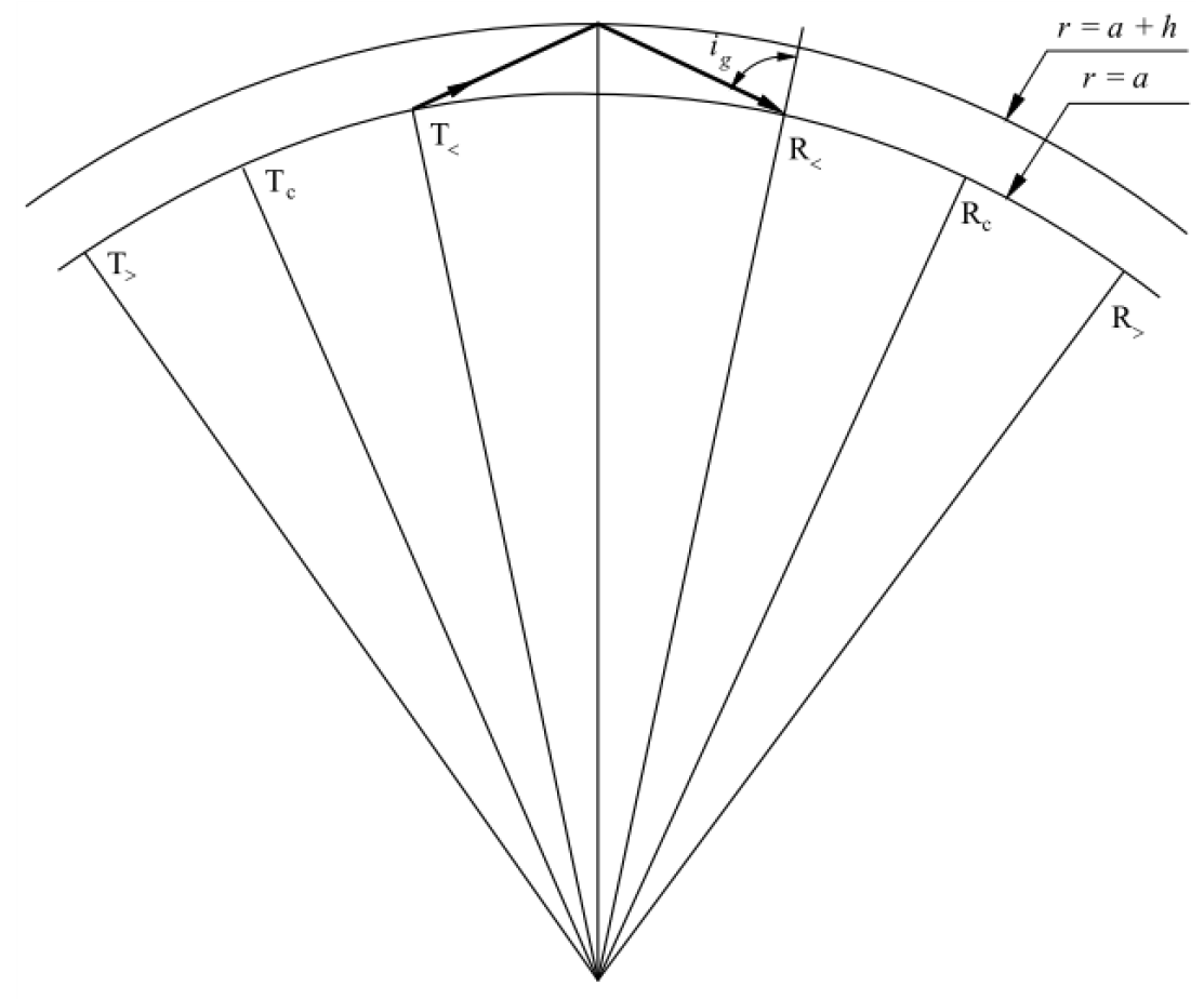
Assuming h represents the ionospheric height and r=a is used to define a smooth Earth's surface, the ionosphere r=a+h is located at a concentric spherical surface [28]. Assuming the transmitting antenna is a short vertical dipole, the signal strength of the electromagnetic wave after reflection by the ionosphere before reaching the ground is:
In the formula, L represents the skywave path length,denotes the ionospheric reflection system, D stands for the ionospheric focusing coefficient, Ft represents the transmitting antenna coefficient, denotes the transmitting and receiving angle, and Vu represents the electric field strength of the transmitting antenna.
3. Measurement Principle and Experimental Design
3.1. Principle of Field Strength Measurement for Low-Frequency Time-Code Signal
Based on the characteristics of low-frequency time-code signal, the signal within the first 400ms after being triggered by a 1PPS signal may all be amplitude drop points. Considering the impact of path delay in radio wave propagation, the data within the first 500ms may all be amplitude drop points (a path delay of 100ms corresponds to a propagation distance of 30,000km, which is much larger than the coverage range of a low-frequency time code timing station). Therefore, when calculating field strength, the first 500ms of sampled data per second are discarded, and only the signals within the last 500ms per second are retained. At this time, the signal is a sine signal with a single frequency.
To minimize the impact of interference on measurement results, the data involved in the calculation is first transformed into the frequency domain through FFT. Assuming the sampling frequency is Fs and the number of sampling points is N, after FFT transformation, the frequency represented by a certain point n (n starts from 1) is:
By dividing the amplitude spectrum modulus at this point by the front-end amplification factor, i.e., N/2, we can obtain the amplitude of the signal at this frequency, which is:
In the formula, AFs represents the signal amplitude, and denotes the Fn amplitude spectrum modulus.
Based on the above analysis, the field strength measurement process for low-frequency time-code signal is shown in Figure 2. The induced electrical signal on the antenna is amplified, filtered, and subjected to FFT transformation. After that, synchronous sampling is performed under the trigger of a standard 1PPS second signal, with a sampling frequency of Fs. The amplitude spectrum modulus of is calculated to obtain the amplitude of the sampled signal. By dividing this value by the amplification factor N/2 of the front-end signal, the amplitude value of the signal can be obtained. Considering the system errors such as transmission cable loss between the receiving antenna and the measuring instrument, the field strength value can be calculated after deducting these errors. The formula for calculating the field strength is as follows:
Where, E is the signal field strength value, AFs is the signal amplitude value, K is the receiving antenna factor, and L is the attenuation value of the transmission cable and other accessories.
3.2. Principle of Time Deviation Measurement for Low-Frequency Time-Code Signal
Based on the characteristics of low-frequency time-code timing streams, the various time delays of low-frequency time-code can be divided into four parts, as shown in the Figure 3. UTC(NTSC) is the standard time generated by the National Time Service Center, and the time delay between it and the UTC is τ0; the time delay between the low-frequency time-code transmitting station and UTC(NTSC) is τ1, which is the traceability time delay, and the low-frequency time-code transmitting station itself has a transmitting control time delay τ2; the signal propagation time delay is τ3; the low-frequency time-code receiver channel time delay is τ4 ; and the total time delay of the entire low-frequency time-code signal propagation is τ.
According to Figure 3, assuming the deviation from BIPM is not considered, if the time of the low-frequency time-code transmitting station is BPCt, then:
Then, the time of the low-frequency time-code receiver can be calculated using the following formula:
Combining Equations (6) and (7), the low-frequency time-code timing model can be expressed as:
3.2. Data Source
The signal monitoring data used in this study sourced from the time service signal monitoring station in Xi'an, Shaanxi Province, China. The geographical location of Xi'an Station is approximately 670 km away from the time signal transmission station, belonging to the interference zone of sky waves and ground waves. Therefore, the Xi'an station can ensure that the sky wave signal can be stably received, and the fluctuation in signal amplitude can effectively reflect changes in sky wave conditions.
At the same time, the timing deviation data involved in the experimental data acquisition requires a standard time-frequency signal as a reference during acquisition. The UTC (NTSC) 1PPS provided by the National Time Service Center, Chinese Academy of Sciences to Xi'an Station provides necessary conditions for collecting timing deviation data. It should be noted that the time service signal uses negative pulse amplitude modulation to transmit time information. In the area where both sky wave and ground wave can be received at the same time, the signal obtained at the receiving end is the superposition of the two. Due to the limitation of the modulation method, in the area where the sky wave and the ground wave act together, the two cannot be separated effectively, so the phase of the received signal is actually the synthesized phase after the fusion of the sky wave and the ground wave, instead of the pure phase of the sky wave.
As can be seen from Figure 4, the measurement equipment, on one hand, completes the reception of low-frequency time-code signals through the receiving antenna and performs field strength measurements. On the other hand, it demodulates 1PPS signals and measures time deviations using a high-precision time interval counter, providing authentic and reliable data for the entire experiment.
4. Data Processing Strategies and Analysis
4.1. Field Strength Data Analysis
Figure 5 shows the field strength measurement data of low-frequency time-code signal for a total of six days from November 10 to November 15, 2025. To ensure the accuracy of measurement data, test data is collected from 10:00 to 15:00 every day. During this period, the ionosphere is in a stable state, which can minimize the interference of other factors on the signal. The measuring equipment fully captured the data on the changes in the field strength of the low-frequency time-code signal.
As can be seen from Figure 5, through analyzing the field strength data of low-frequency time-code signal, it is observed that the field strength fluctuates with time and the receiving environment. The field strength data on November 12th (represented by the red curve in the figure) has a lower mean value compared to other dates. Table 1 displays the statistical results of signal field strength from November 10th to November 15th, 2025. Upon analysis, it was found that the signal field strength on November 12th decreased over 2.3dBμV/m compared to the previous and following two days.
4.2. Time Deviation Data Analysis
Figure 6 shows the time deviation measurement data of low-frequency time-code signal for six days from November 10 to November 15, 2025. Similar to signal field strength testing, to ensure the accuracy of measurement data, test data is collected from 10:00 to 15:00 every day.
As can be seen from Figure 6, through analyzing the time difference data of low-frequency time-code signal, the mean and standard deviation of the time deviation data on November 12 (represented by the red curve in the figure) are relatively large, exhibiting a more dispersed characteristic. Table 2 presents the statistical results of time differences from November 10 to November 15, 2025. Upon analysis, it was found that compared to the previous and following two days, the time difference on November 12 increased over 2.4ms.
5. Discussion
Based on the experimental data above, it can be observed that the signal field strength and time difference data on November 12, 2025, exhibit phenomena different from those on other dates. The signal field strength decreased, while the time difference data increased and multiple discrete points appeared. To verify whether the changes in the above data are caused by geomagnetic storms triggered by solar activity, it is necessary to analyze and comprehensively determine them in conjunction with solar activity data, Dst data, and so on.
5.1. Solar Activity Data
Table 3 presents the solar activity data from November 10 to November 15, 2025. Upon analyzing the data in the table, it is observed that the number of solar rotation cycles during this week is 2622. Both the number of sunspots and the 10.7cm radio flux exhibit similar trends, with both values being high simultaneously, indicating frequent solar activity.
5.2. Dst Data
The geomagnetic index used at stations at mid- and low-latitudes is called the Dst index. This index is measured hourly and primarily indicates the intensity variation of the horizontal component of the geomagnetic field. Figure 7 shows the Dst data for November 2025 (data sourced from the Kyoto Geomagnetic Center). Table 4 presents the Dst data from November 10 to November 15, 2025. Analysis of the data in Table 4 reveals that on November 12, 2025, the Dst data showed a significant increase and remained at a high level, with a maximum value of -209 (nT). It can be inferred that a magnetic storm occurred at this time.
Figure 8 and Figure 9 respectively show the changes in signal field strength and time deviation data from November 10 to November 15, 2025, as a function of Dst data fluctuations. It should be noted that due to the fact that the Shangqiu low-frequency time-code station does not broadcast signals from 05:00 to 08:00 every day, the invalid data in this segment has been removed during data processing, and the data in other time periods are all original measurement data.
From Figure 8, it can be seen that the Dst data from November 10th to November 11th remained relatively stable, with violent fluctuations starting from November 12th and reaching a maximum of -209nT on November 12th. The average signal field strength on that day was 59.9634dBμV/m, a decrease of more than 2.3 dBμV/m compared to the previous two days. when the Dst value increased significantly on November 12th, the geomagnetic field underwent drastic changes, and the signal field strength and time deviation also changed accordingly
From Figure 9, it can be seen that when the Dst data began to fluctuate violently on November 12th, there were a large number of outliers in the time deviation measurement values, and they showed a highly discrete state. According to statistics, on November 12th alone, there were 152 invalid data points, accounting for 2.1% of the total day's data. This has had a certain impact on the timing performance of low-frequency time-code signal.
5.3. Kp Index and AE Index
Generally speaking, the geomagnetic index is a grading indicator that describes the intensity of geomagnetic disturbances within each time period, or a physical quantity that indicates the intensity of a certain type of magnetic disturbance (see Earth's variable magnetic field). The time intervals are divided according to Universal Time. In this article, we choose the first type of index to describe the overall level of geomagnetic activity, regardless of the specific type of magnetic disturbance, including the C and Ci indices, k and kp indices, Ak and Ap indices, etc. We have queried the geomagnetic data from November 10 to November 15, 2025, as shown in Table 5.
The Kp index is an index used by a single geomagnetic observatory to describe the intensity of geomagnetic disturbances within each 3-hour period each day, known as the three-hour index or magnetic condition index. By analyzing the data in Table 5, it is found that the total sum of the Kp index for the entire day on November 12 was 357, and it remained at a high value throughout the day, proving the occurrence of geomagnetic disturbances in the area where the test point is located. Similar to the trend shown in Figure 8 and Figure 9, when the Kp value increased significantly on November 12th, the signal field strength and time deviation also changed accordingly.
The AE index represents the sum of the absolute values of the maximum positive change (AU index) and the maximum negative change (AL index) within each hour.
By analyzing the data in Figure 10, it is observed that during the period from November 12th to November 13th, the AL index exhibited a rapid growth trend, meanwhile, the minimum value on November 12th has exceeded -2000(nT), indicating a significant increase in the solar wind containing charged particle streams at that time.
5.4. Analysis of Low-Frequency Time-Code Signal Changes During Geomagnetic Storms
After analyzing solar activity data, Dst data, and Kp data separately, we can preliminarily determine that the low-frequency time-code signal was affected by a geomagnetic storm on November 12, 2025, resulting in a decrease in field strength and an increase in time deviation. The reasons for this are as follows:
(1) Regarding signal field strength, due to the influence of solar activity, the ionization degree of ions and electrons in the lower ionosphere is enhanced, and the healing speed of the ionosphere gradually slows down. This results in small daily data fluctuations during geomagnetic storms, but the overall trend remains relatively stable, without any extreme maximum or minimum values, and the numerical changes are also within a reasonable range.
(2) Regarding time deviation, as the local magnetic data increases, there will be greater fluctuations in the low-frequency time-code timing deviation data and an increase in time deviation. This is because the equivalent emission height of the low ionosphere gradually decreases on the propagation path of the low-frequency time-code signal. When the signal passes through the D layer, the attenuation of the signal increases and phase delay occurs, resulting in an increase in time deviation. After the local magnetic data gradually returned to normal, the equivalent reflection height of the low ionosphere gradually increased, and the time deviation slowly returned to the reference day situation.
6. Conclusions
This paper regards the geomagnetic storm phenomenon that occurred from November 10 to November 15, 2025, and the testing team established a signal monitoring system in Xi'an, Shaanxi Province, using low-frequency time-code signal as an example. They conducted detailed tests on the field strength and time deviation of signal. Through detailed analysis of the measured data, the testing team can draw the following conclusions:
(1) When the high-speed solar wind or coronal mass ejection generated by solar eruptions impacts the Earth, it can cause drastic changes in the Earth's magnetic field within a short period of time. For low-frequency time code timing signals that rely on ionospheric reflection for long-distance transmission, this phenomenon can lead to a decrease in signal field strength and an increase in time deviation. The reason behind this is that as the signals pass through the D layer, the degree of ionization in the ionosphere increases [29], and the equivalent emission height of the lower ionosphere gradually decreases [30], resulting in increased signal attenuation and phase delay, which leads to a larger time difference.
(2) Thanks to the propagation characteristics of low-frequency signals, low-frequency time-code timing signals exhibit a certain degree of anti-interference capability during geomagnetic storms. This capability is primarily manifested in the power level of the signals within the coverage area. The higher the power, the stronger the anti-interference capability. During geomagnetic storms, the overall signal field strength remains relatively high (with a minimum of 58.8577dBμV/m on November 12th), it can basically ensure normal reception for users within the coverage area. This is also related to the fact that during geomagnetic storms, solar mass ejections shift towards the poles along magnetic field lines, without continuously affecting the ionosphere directly above the receiving point.
(3) Lastly, it should be noted that in this observation experiment, when the transmitting power of the transmitter remains constant, the low-frequency time code timing signal, which relies on skywave reflection for long-distance propagation, will also undergo corresponding changes when the ionosphere changes. Both the signal field strength and time deviation will be affected by changes in the geomagnetic field. For the low-frequency time code timing system, how to consider targeted countermeasures when the ionosphere undergoes drastic changes to ensure that the timing signal is not affected becomes a question that we need to consider next.
Author Contributions
X.W. designed the mathematical model of the proposed algorithm and wrote the article; F.Z. performed the experiments and completed the data preprocessing, X.R. and P.F. analyzed the test data, S.Z and X.L. helped to frame the idea. All authors have read and agreed to the published version of the manuscript.
Funding
This research was funded by Guangdong Provincial Science and Technology Plan Project, NO.2019B090904006.
Data Availability Statement
The Low-Frequency time-code signal strength data and time deviation data can be accessed through the Comprehensive Monitoring Platform of the Timing System at the National Time Service Center , Chinese Academy of Sciences. According to the confidentiality regulations of the National Time Service Center, external individuals and institutions are not granted access. External researchers can contact the National Time Service Center (http://english.ntsc.cas.cn/) to submit a reasonable request for authorization. Once authorized, the corresponding author will access the data on their behalf. Solar activity data is provided by British Geological Survey (BGS), and the data source can be accessed at http://www.geomag.bgs.ac.uk/data_service/space_weather/home.html. Dst data, Kp data and AE data is provided by Kyoto Geomagnetic Center, and the data source can be accessed at https://wdc.kugi.kyoto-u.ac.jp/.
Acknowledgments
The authors would like to thank their colleagues for the testing of the data provided in this manuscript. We are also very grateful to our reviewers who provided insight and expertise that greatly assisted the research.
Conflicts of Interest
The authors declare no conflict of interest.
Abbreviations
The following abbreviations are used in this manuscript:
| IGS | International GNSS Service |
| GPS | Global Positioning System |
| TEC | Total Electron Content |
| GAGAN | GPS-aided Augmented Navigation |
| GIC | Ground Induced Current |
| LEO | Low Earth Orbit |
| VLEO | Very Low Earth Orbit |
| PPS | Pulse Per Second |
| FFT | Fast Fourier Transform |
References
- Zehra Can·Hasan ¸ Safak Erdag˘, Effect of Solar Parameters on Geomagnetic Storm Formation in the Ascending Phase of the 25th Solar Cycle. Solar Physics 2025, 300, 20. [CrossRef]
- ÇİFTÇİ, E; HACIOĞLU, Ö. Geomagnetic activity for the Kp = 7.3 geomagnetic storm in November 2023 assessed by observational data. Turkish Journal of Earth Sciences 2025, 34(6), 724–733. [Google Scholar] [CrossRef]
- Yuxuan,Zhu, Modeling And Analysis Of Geoelectric Fields During Geomagnetic Storms, Master Thesis of Harbin Institute of Technology,2025.01.
- Meng Sun, Research on the Response of Temperature and Density in the Mesosphere-Lower Thermosphere to Geomagnetic Storms, Doctoral Dissertation of Nanjing University of Information Science and Technology, 2025.06.
- LI Site, JIANG Guangxin, HAN Jinsi, XIE Zongtao, GAO Xuelian, LIU Lianguang, Geomagnetic Disturbance Impact on Transformers in AC/DC UHV Stations of the Ximeng Power Grid, Power System Technology, 2025.
- Chen Yi, Rui Zhang, Analysis of the Impact of Geomagnetic Storms on Pseudorange Single Point Positioning, Modern navigation, NO.4,2024.
- Liu, WANG; Lizhi, LOU; Ling, YANG. Impact of geomagnetic storms on GNSS positioning performance and data quality. Beijing Surveying and Mapping 2025, 39(8), 121 8–1224. [Google Scholar]
- Ramana, G. Venkata; Sridhar, M.; Rao, T. Venkateswara; Ratnam, D. Venkata. Superposed epoch analysis of GPS ionospheric TEC and scintillations over low latitude Indian region during multiple geomagnetic storm events. Earth Science Informatics 2025, 18, 51. [Google Scholar] [CrossRef]
- Lawrence, E; Beggan, CD; Richardson, GS; Reay, S; Thompson, V; Clarke, E; Orr, L; Hübert, J; Smedley, ARD. The geomagnetic and geoelectric response to the May 2024 geomagnetic storm in the United Kingdom. Front. Astron. Space Sci. 2025, 12, 1550923. [Google Scholar] [CrossRef]
- Yu, H.; Chen, L.; Chen, B. Impact of Solar Irradiance on Low-Earth-Orbit Satellite Orbital Decay During Geomagnetic Storm. Aerospace 2025, 12, 1084. [Google Scholar] [CrossRef]
- Denny M. Oliveira, Eftyhia Zesta, Dibyendu Nandy, The 10 October 2024 geomagnetic storm may have caused the premature reentry of a Starlink satellite, Physics.space-ph(19 Dec 2024),doi: arXiv:2411.01654v2.
- Li, S Y; Ren, Z P; Yu, T T; et al. Study of the thermospheric responses over Beijing during the geomagnetic storm on December 1-2, 2023[J]. Chinese Journal of Geophysics 2025, 68(6), 2028–2038. [Google Scholar]
- Hongyu, ZHAO; Shuhua, ZHOU; Yingcai, KUANG; Ning, WANG. Global Ionospheric Response to the Geomagnetic Storms from March to April 2023. Chinese Journal of Space Science (in Chinese). 2025, 45(5), 1220–1229. [Google Scholar] [CrossRef]
- Idosa Uga, Chali; Uluma, Edward; Adhikari, Binod; Giri, Ashutosh; Belay, Negasa. Impact of the October 28, 2021 Solar Flare and the November 4,2021 Geomagnetic Storm on the Low, Middle, and High-Latitude Ionosphere. Discover Space 2024, 128, 4. [Google Scholar] [CrossRef]
- Nayak, C.; Buchert, S.; Yiğit, E.; Ankita, M.; Singh, S.; Tulasi Ram, S.; Dimri, A. P. Topside low-latitude ionospheric response to the 10–11 May 2024 super geomagnetic storm as observed by Swarm: The strongest storm-time super-fountain during the Swarm era? Journal of Geophysical Research: Space Physics 2025, 130, e2024JA033340. [Google Scholar] [CrossRef]
- Wang Shang, Lou Guangzhen,Ionospheric monitoring during geomagnetic storms and analysis of perturbation under different GNSS observation modes, Geotechnical Investigation & Surveyina,NO 6,2024.
- Qi, Z.; Huang, L.; Wang, X.; Zhao, F.; Cheng, L.; Liu, Q.; et al. Research on the impact of differences in solar flare backgrounds of the same-class on low-frequency time code time service signal. Journal of Geophysical Research:Space Physics 2025, 130, e2025JA033801. [Google Scholar] [CrossRef]
- Qi, Z.; Ren, X.; Liu, Q.; Zhao, F.; Huang, L.; Chen, Y.; et al. Study on thevariation of low-frequency time code signals during medium to large solar flare events. Radio Science 2025, 60, e2024RS008186. [Google Scholar] [CrossRef]
- ITU-R,P.368-9,Ground-Wave Propagation Curvrs for Frequencies between 10kHz and 30MHz, 2007.
- ITU-R,P.684-7,Prediction of field strength at frequencies below about 150 kHz,2016.
- Liu Jun, The theory and the technique of engineering on low-frequency time-code in time service system[D].Graduate University of Chinese Academy of Sciences,2002.
- BAI Chun-hui, Method to Enhance Veracity of Measuring Radio Signal's Electric Field Intensity[J]. COMMUNICATION COUNTERMEASURES, 2007.3:62-64.
- Tianming, Xiang. Television Signal Field Strength Measurement and Air Manage-ment[J]. CHINA CABLE TELEVISION 2002, 10, 48–50. [Google Scholar]
- Yuan, Zhang. Method and Application of Field Intensity of Medium and Short Wave Broadcasting Signal[J]. INFORMATION SYSTEM ENGINEERING 2019, 2, 88. [Google Scholar]
- Xin, Dong. Analysis on the Key Problems of Field Strength Measurement of FM TV[J]. Wireless Internet Technology 2016, 4, 3–5. [Google Scholar]
- Wakai, Noboru; Kurihara, Noriyuki; Otsuka, Atsushi; Imamura, Kuniyasu; Takahashi, Yukio. Wintertime survey of LF field strengths in Japan. RADIO SCIENCE 2006, VOL. 41, RS5S13. [Google Scholar] [CrossRef]
- Wang Na, Study on Field Strength and Delay of Low frequency Ground-wave[D]. Graduate University of Chinese Academy of Sciences,2012.
- Wei Xu, Robert A. Marshall, Antti Kero, Esa Turunen, Douglas Drob, Jan Sojka, and Don Rice, VLF Measurements and Modeling of the D-Region Response to the 2017 Total Solar Eclipse, IEEE TRANSACTIONS ON GEOSCIENCE AND REMOTE SENSING, P1-P10, 2019.
- Jiang, Huang; Baichang, Deng; Jie, Xu; Linfeng, Huang; Weifeng, Liu; Wenhua, Zhao. Study of the South China ionospheric TEC disturbances during June-July 2009. Chin. J. Space Sci. 2011, 31(6), 739–746. [Google Scholar] [CrossRef]
- Bai-xian, Liang; Jun, Li; Shu-ying, Ma. PROGRESS OF IONOSPHREIC RESREACH IN CHINA. ACTA GEOPHYSICA SINICA 1994, Vol.37, Supp.1. [Google Scholar]
Figure 2.
Field strength measurement process.
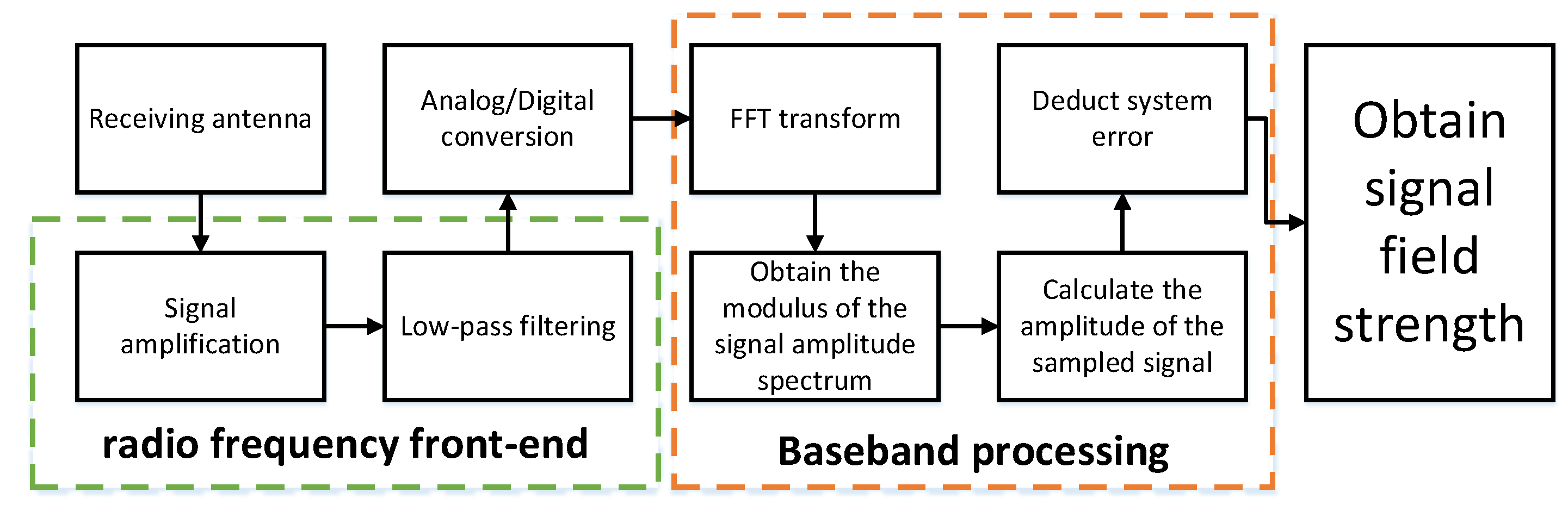
Figure 3.
Various time delays of low-frequency time-code.
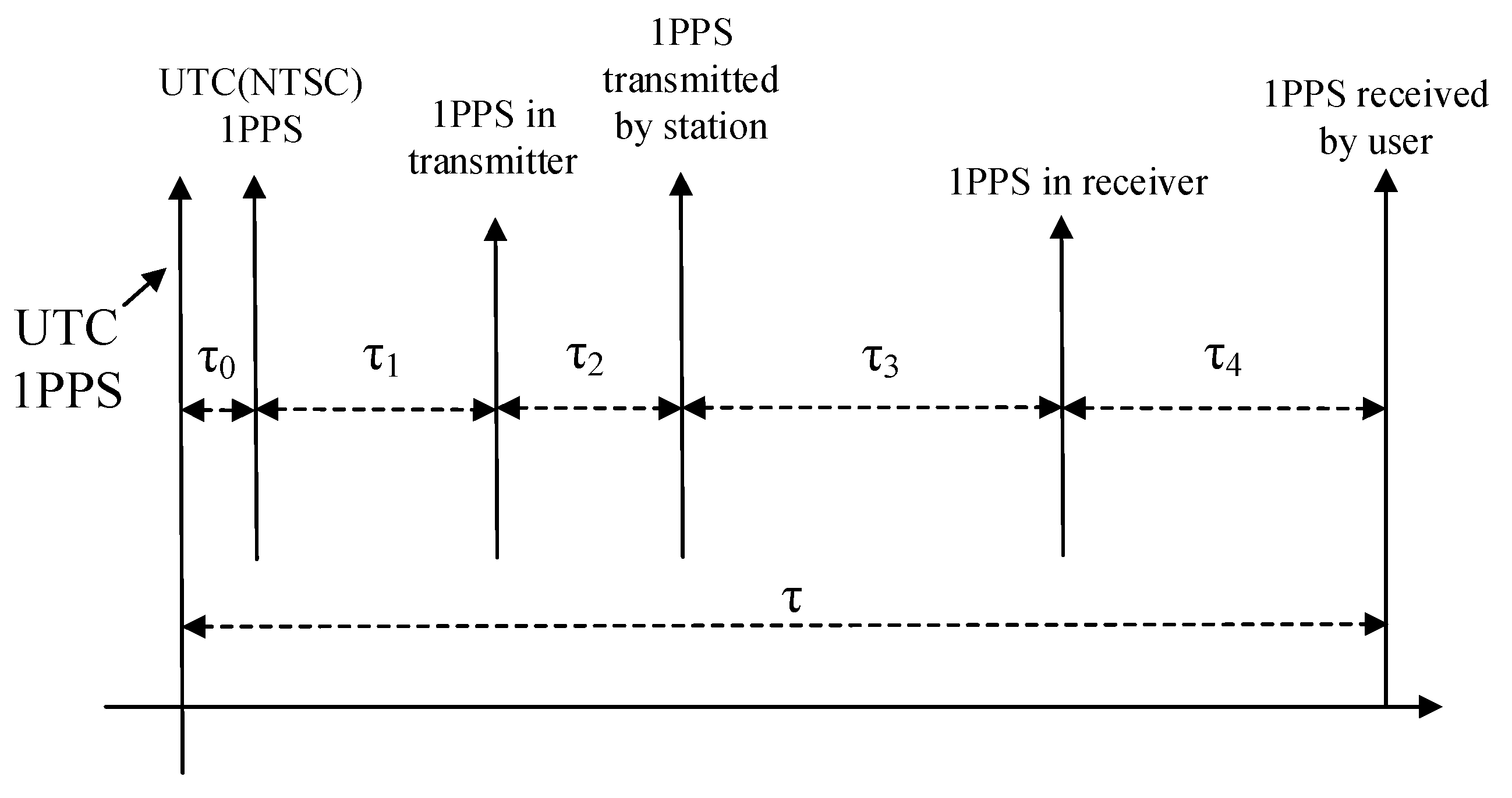
Figure 4.
Signal measurement principle and instrument.
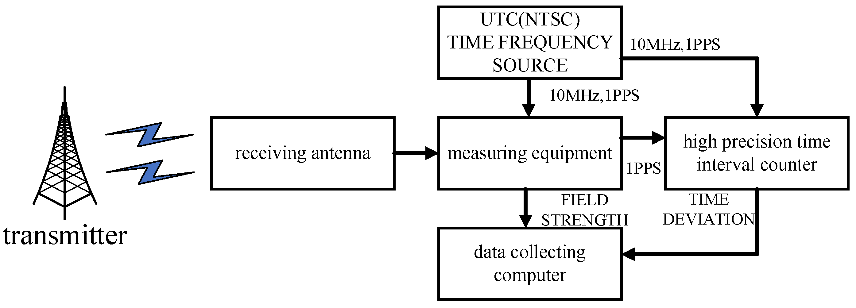
Figure 5.
Field strength measurement data from November 10 to November 15, 2025.
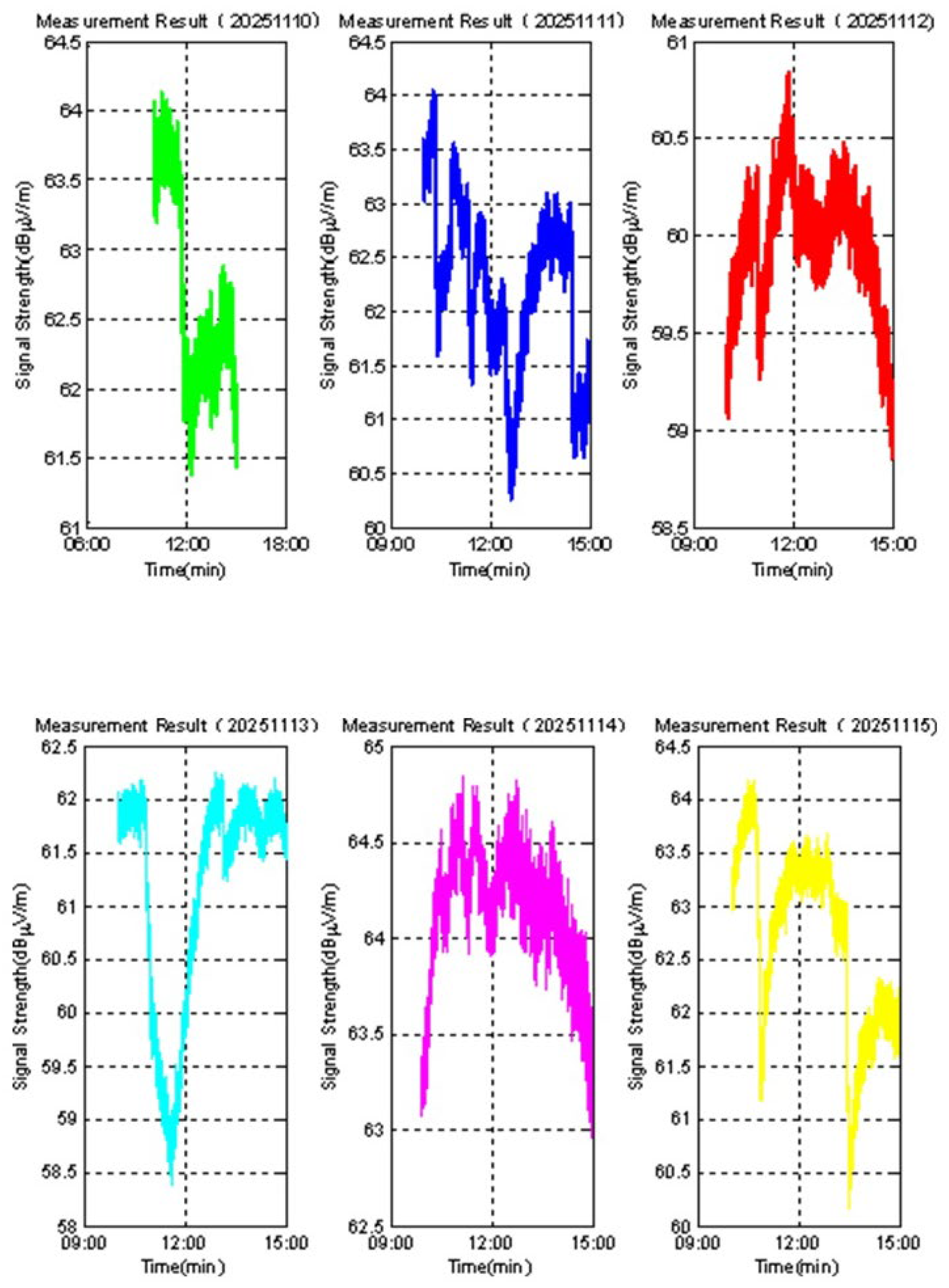
Figure 6.
Time deviation measurement data from November 10 to November 15, 2025.
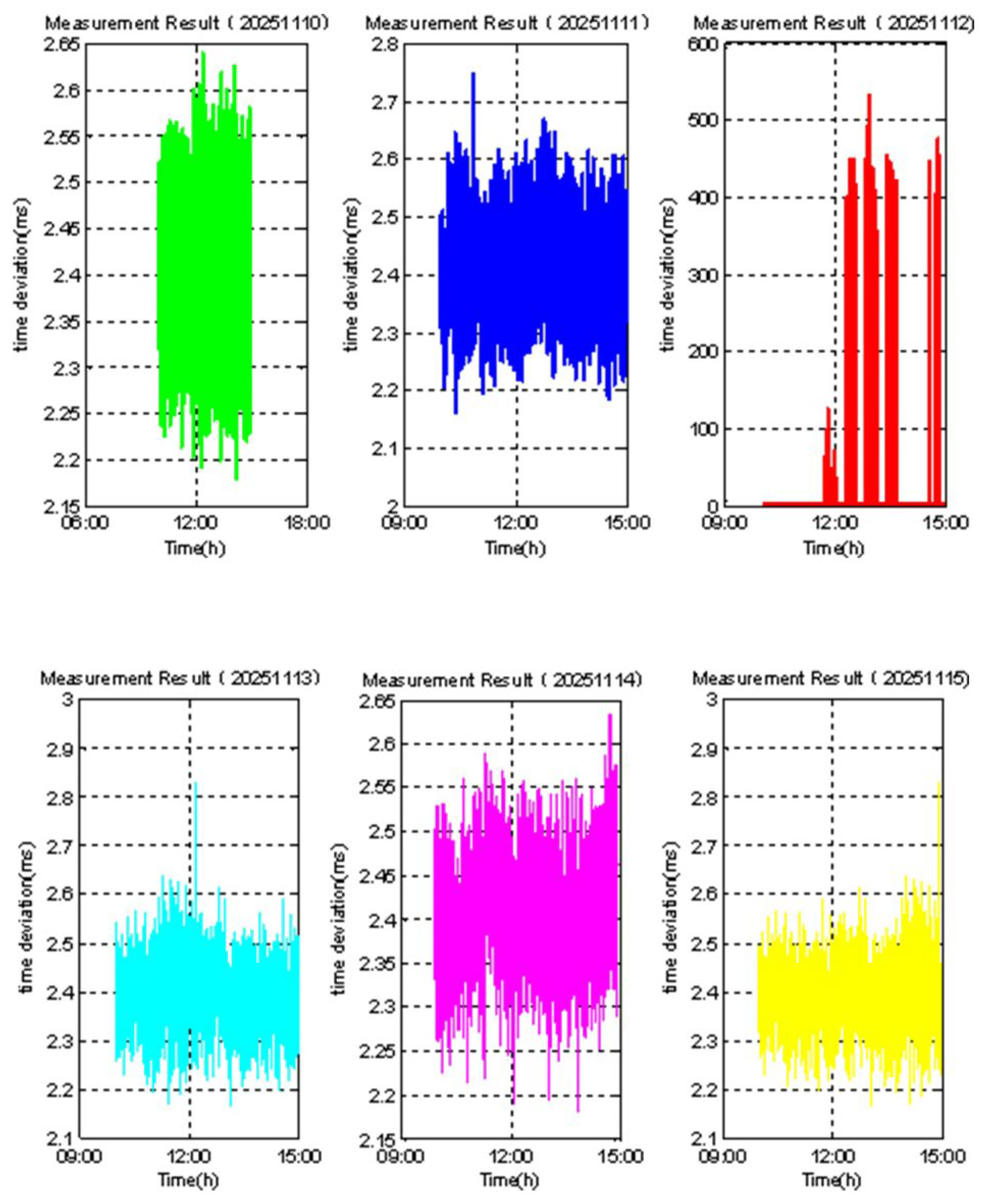
Figure 7.
Dst data in November 2025 (data sourced from Kyoto Geomagnetic Center https://wdc.kugi.kyoto-u.ac.jp/wdc/Sec3.html ).
Figure 7.
Dst data in November 2025 (data sourced from Kyoto Geomagnetic Center https://wdc.kugi.kyoto-u.ac.jp/wdc/Sec3.html ).
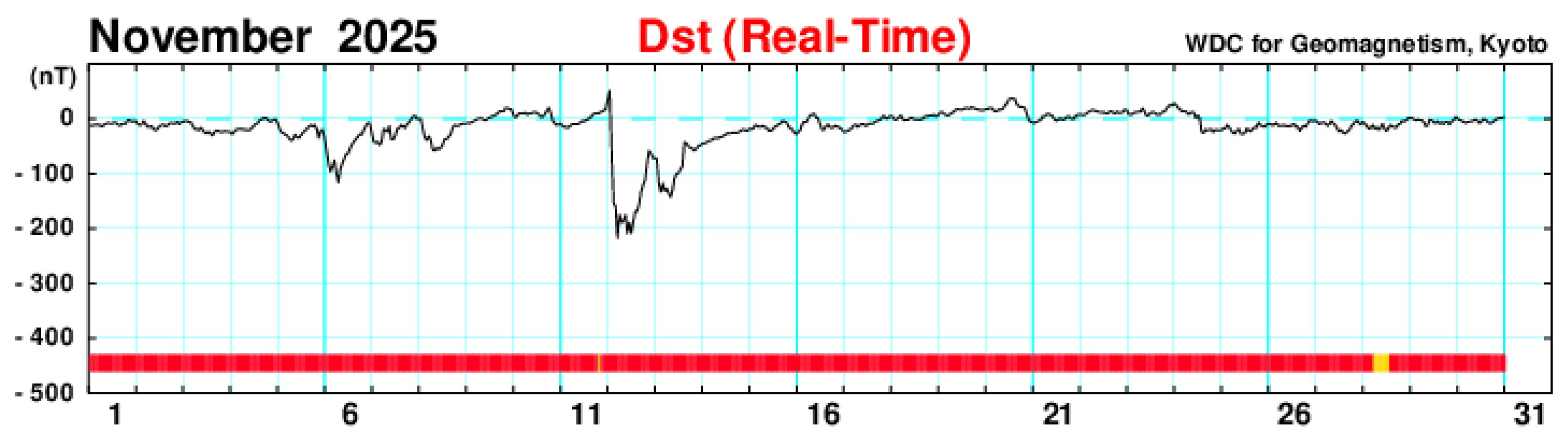
Figure 8.
Signal measurement principle and instrument.
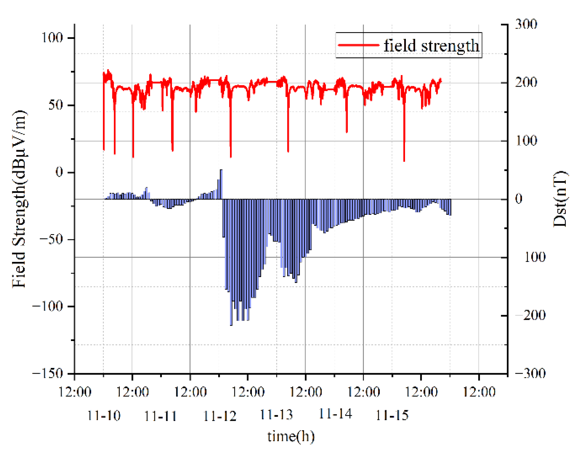
Figure 9.
Signal measurement principle and instrument.
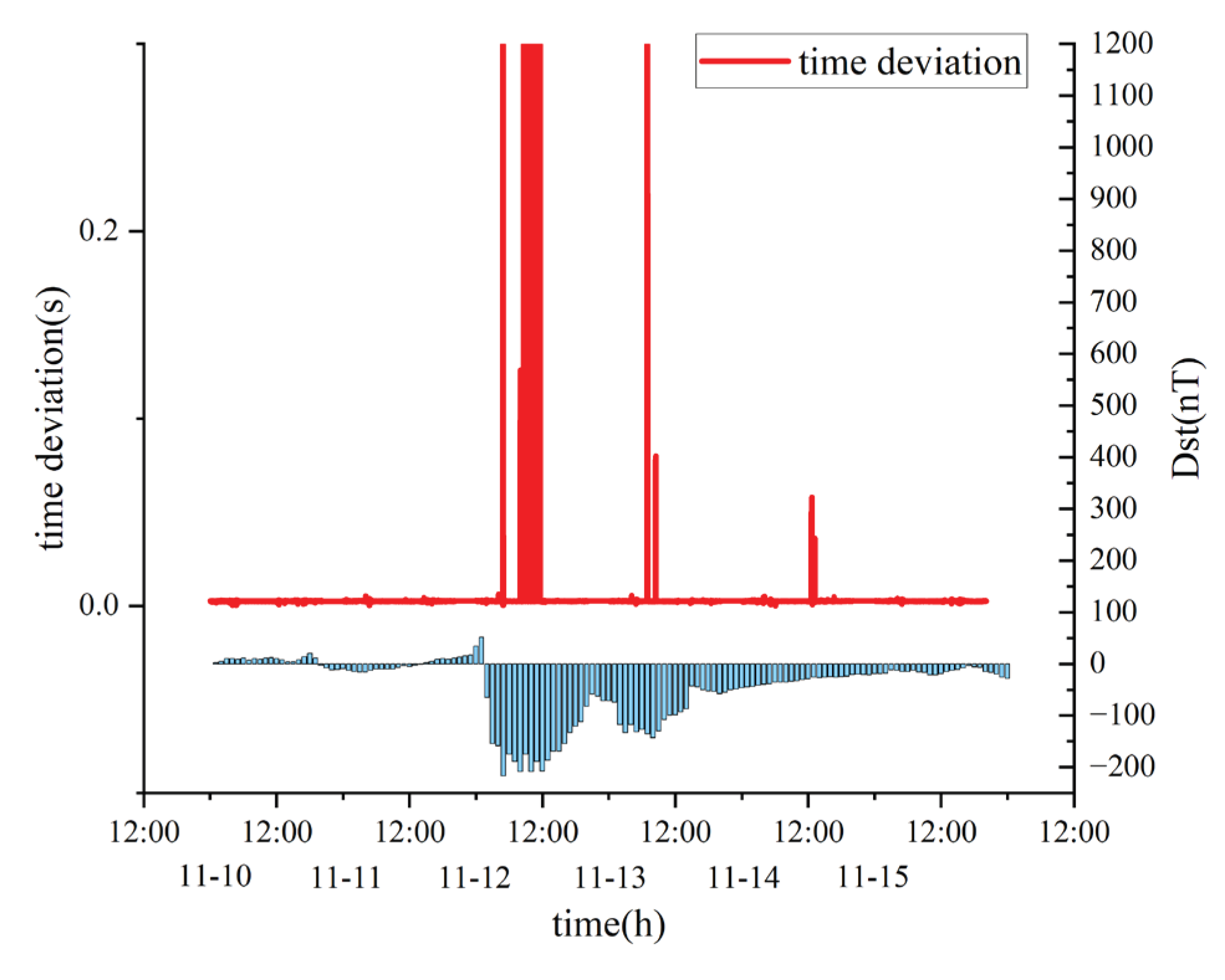
Figure 10.
AE data from November 10 to November 15, 2025 (data sourced from Kyoto Geomagnetic Center https://wdc.kugi.kyoto-u.ac.jp/wdc/Sec3.html).
Figure 10.
AE data from November 10 to November 15, 2025 (data sourced from Kyoto Geomagnetic Center https://wdc.kugi.kyoto-u.ac.jp/wdc/Sec3.html).
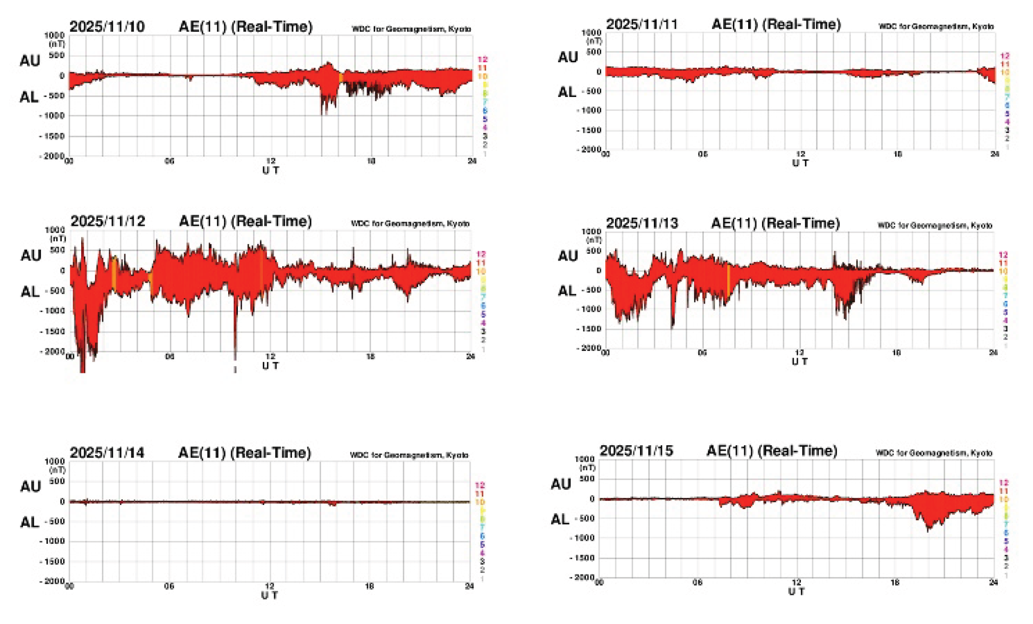

Table 1.
Statistical results of signal field strength from November 10 to November 15, 2025.
|
Mean (unit: dBμV/m) |
Std (unit: dBμV/m) |
Max (unit: dBμV/m) |
Min (unit: dBμV/m) |
|
| 20251110 | 62.6824 | 0.7194 | 64.1304 | 61.3747 |
| 20251111 | 62.2317 | 0.7599 | 64.0425 | 60.2554 |
| 20251112 | 59.9634 | 0.314 | 60.8444 | 58.8577 |
| 20251113 | 62.9778 | 1.0351 | 64.0539 | 60.1796 |
| 20251114 | 64.1549 | 0.3141 | 64.8526 | 62.9625 |
| 20251115 | 62.6825 | 0.8575 | 64.1850 | 60.1727 |
Table 2.
Statistical results of time deviation from November 10 to November 15, 2025.
|
Mean (unit: ms) |
Std (unit: ms) |
Max (unit: ms) |
Min (unit: ms) |
|||
| 20251110 | 2.4094 | 0.0596 | 2.6391 | 2.1802 | ||
| 20251111 | 2.4128 | 0.0686 | 2.7458 | 2.1618 | ||
| 20251112 | 4.8114 | 30.7244 | 533.7450 | 2.1807 | ||
| 20251113 | 2.3937 | 0.0613 | 2.8318 | 2.1677 | ||
| 20251114 | 2.4083 | 0.0546 | 2.6347 | 2.1797 | ||
| 20251115 | 2.3645 | 0.0523 | 2.8272 | 2.1588 | ||
Table 3.
Solar activity data from November 10 to November 15, 2025.
| Date | Solar Rotation number |
Day into Solar Cycle |
International Sunspot Number | 10.7cm Flux | Flux Qualifier |
| 20251110 | 2622 | 2 | 154 | 176.8 | 0 |
| 20251111 | 2622 | 3 | 155 | 164.7 | 0 |
| 20251112 | 2622 | 4 | 143 | 160.0 | 0 |
| 20251113 | 2622 | 5 | 134 | 152.7 | 0 |
| 20251114 | 2622 | 6 | 105 | 142.2 | 0 |
| 20251115 | 2622 | 7 | 105 | 129.4 | 0 |
Table 4.
Dst data from November 10 to November 15, 2025.
| Dst(unit=nT),NOVEMBER,2025 | ||||||
| 20251110 | 20251111 | 20251112 | 20251113 | 20251114 | 20251115 | |
| 1:00 | 2 | -13 | 51 | -74 | -45 | -19 |
| 2:00 | 5 | -15 | -65 | -118 | -44 | -18 |
| 3:00 | 10 | -16 | -155 | -133 | -41 | -12 |
| 4:00 | 10 | -16 | -159 | -118 | -40 | -13 |
| 5:00 | 9 | -13 | -217 | -132 | -39 | -15 |
| 6:00 | 11 | -10 | -175 | -127 | -36 | -15 |
| 7:00 | 7 | -10 | -189 | -136 | -36 | -13 |
| 8:00 | 10 | -10 | -209 | -143 | -36 | -16 |
| 9:00 | 9 | -10 | -175 | -130 | -34 | -17 |
| 10:00 | 11 | -7 | -209 | -108 | -33 | -22 |
| 11:00 | 12 | -4 | -189 | -100 | -31 | -22 |
| 12:00 | 10 | -5 | -208 | -99 | -29 | -19 |
| 13:00 | 8 | -3 | -187 | -93 | -26 | -15 |
| 14:00 | 4 | -1 | -169 | -87 | -27 | -13 |
| 15:00 | 4 | 2 | -169 | -43 | -26 | -11 |
| 16:00 | 8 | 5 | -155 | -45 | -25 | -8 |
| 17:00 | 14 | 9 | -133 | -50 | -26 | -4 |
| 18:00 | 20 | 10 | -121 | -53 | -25 | -6 |
| 19:00 | 11 | 9 | -112 | -54 | -24 | -7 |
| 20:00 | -3 | 11 | -82 | -58 | -21 | -15 |
| 21:00 | -8 | 13 | -59 | -55 | -20 | -17 |
| 22:00 | -12 | 15 | -63 | -50 | -21 | -20 |
| 23:00 | -11 | 17 | -72 | -49 | -22 | -26 |
| 24:00 | -9 | 34 | -72 | -46 | -19 | -28 |
Table 5.
Dst data from November 10 to November 15, 2025.
| Date | Kp: Planetary 3Hr Range Index | Sum Kp | ap: Planetary Equiv. Amplitude |
A p |
C p |
C9 | ||||||||||||||
| 20251110 | 27 | 20 | 10 | 20 | 30 | 40 | 30 | 33 | 210 | 12 | 7 | 4 | 7 | 15 | 27 | 15 | 18 | 13 | 0.8 | 4 |
| 20251111 | 17 | 23 | 13 | 20 | 3 | 7 | 3 | 27 | 113 | 6 | 9 | 5 | 7 | 2 | 3 | 2 | 12 | 6 | 0.3 | 1 |
| 20251112 | 87 | 83 | 73 | 77 | 57 | 43 | 57 | 40 | 517 | 300 | 236 | 154 | 179 | 67 | 32 | 67 | 27 | 133 | 1.9 | 8 |
| 20251113 | 67 | 73 | 63 | 37 | 47 | 33 | 27 | 10 | 357 | 111 | 154 | 94 | 22 | 39 | 18 | 12 | 4 | 57 | 1.7 | 7 |
| 20251114 | 10 | 3 | 7 | 13 | 10 | 10 | 3 | 0 | 57 | 4 | 2 | 3 | 5 | 4 | 4 | 2 | 0 | 3 | 0.1 | 0 |
| 20251115 | 17 | 10 | 20 | 20 | 17 | 13 | 30 | 30 | 157 | 6 | 4 | 7 | 7 | 6 | 5 | 15 | 15 | 8 | 0.4 | 2 |
Disclaimer/Publisher’s Note: The statements, opinions and data contained in all publications are solely those of the individual author(s) and contributor(s) and not of MDPI and/or the editor(s). MDPI and/or the editor(s) disclaim responsibility for any injury to people or property resulting from any ideas, methods, instructions or products referred to in the content. |
© 2026 by the authors. Licensee MDPI, Basel, Switzerland. This article is an open access article distributed under the terms and conditions of the Creative Commons Attribution (CC BY) license (http://creativecommons.org/licenses/by/4.0/).
Copyright: This open access article is published under a Creative Commons CC BY 4.0 license, which permit the free download, distribution, and reuse, provided that the author and preprint are cited in any reuse.


