Submitted:
27 January 2026
Posted:
29 January 2026
Read the latest preprint version here
Abstract
We develop a falsifiable effective framework in which the infrared scale enteringholographic dark energy is defined operationally by a quantum-information copying time. For aphysical separation L at cosmic time t, the copy time τcopy (L, t) is the time required to replicatea minimal unit of quantum information across that separation. The copy horizon Lcopy(t) is fixed locally by τcopy(Lcopy, t) = ξ/H(t), with ξ = O(1). Combining this operational infraredscale with the Cohen–Kaplan–Nelson gravitational-collapse bound motivates an energy density ρQ(t) = 3κM2PlcQ(t)/L2copy(t) and promotes “saturation” to a one-sided falsifiable inequality 0 < cQ ≤ 1 (Hard Consistency Bound). We relate τcopy to coarse-grained entropy productionand adopt a late-time diffusion-limited closure τcopy ≈ L2/D∞(t), which closes the backgrounddynamics and yields an analytic expansion history E(z) = H(z)/H0. We describe a late-timelikelihood based on binned Pantheon+ supernovae and SDSS DR16 BAO consensus distances,with the sound horizon treated as a nuisance parameter when desired.
Keywords:
holographic dark energy
; quantum information
; infrared cutoff
; cosmological expansion
; BAO
; supernovae
; structure growth
1. Introduction
Holographic dark energy (HDE) connects an effective vacuum energy density to an infrared (IR) scale while respecting gravitational-collapse constraints. A persistent conceptual issue in several HDE prescriptions is the appearance of teleological scales (e.g., future event horizons). The Quantum Information Copy Time (QICT) approach instead defines the relevant IR scale operationally and locally, by tying it to an information-theoretic clock. The gravitational consistency condition is implemented using the Cohen–Kaplan–Nelson (CKN) argument that an effective field theory in a region of size L should not include states whose total energy would form a black hole [1]. A standard HDE realization is due to Li [2]. This manuscript presents a single self-contained article (no embedded multi-PDF appendices) in layout.
2. Operational Definition of Copy Time and Copy Horizon
For a physical separation L at cosmic time t, define as the time required to replicate a minimal unit of quantum information across that separation. The copy horizon is defined implicitly by
This condition is operational rather than kinematic: it specifies the largest scale over which the information unit can be copied within one “Hubble time”.
2.1. Entropy-Production Clock
A coarse-grained closure relates the copying time to entropy production,
where is a coarse-grained von Neumann entropy and normalizes the minimal information “brick”.
3. Collapse Constraint and the Hard Consistency Bound
The CKN constraint implies , equivalently [1]. Defining the QICT dark-energy sector by
we promote saturation to a falsifiable one-sided inequality,
If a joint fit to cosmological observables demands (for the specified ), then the assumed operational mapping and collapse constraint are mutually inconsistent.
4. Late-Time Closure and Analytic Background Evolution
To obtain a predictive background evolution, the operational definition must be closed by a model for . A late-time diffusion-limited closure takes
Combining with the definition of yields
Substituting into implies in the saturation regime (slowly varying and ). For a flat universe with pressureless matter, this produces the quadratic closure
with fixed by . The resulting analytic solution is
The effective equation of state follows from .
5. Distances, Growth, and Late-Time Likelihood
Given , luminosity distances follow from , and supernova distance moduli can be compared to binned Pantheon+ data with the published covariance (profiling analytically over the nuisance magnitude M). BAO constraints can be implemented using consensus SDSS DR16 distances, treating the sound horizon as a nuisance parameter to avoid importing an early- calibration in a purely late-time fit.
A minimal clustering completion maps the QICT sector to an effective fluid with background and rest-frame sound speed , producing scale-dependent growth. Standard perturbation-theory formalisms may be used as in [3].
6. Representative Figures
Figure 1.
Reconstruction of at an illustrative best-fit point (QICT vs. a flat CDM reference).
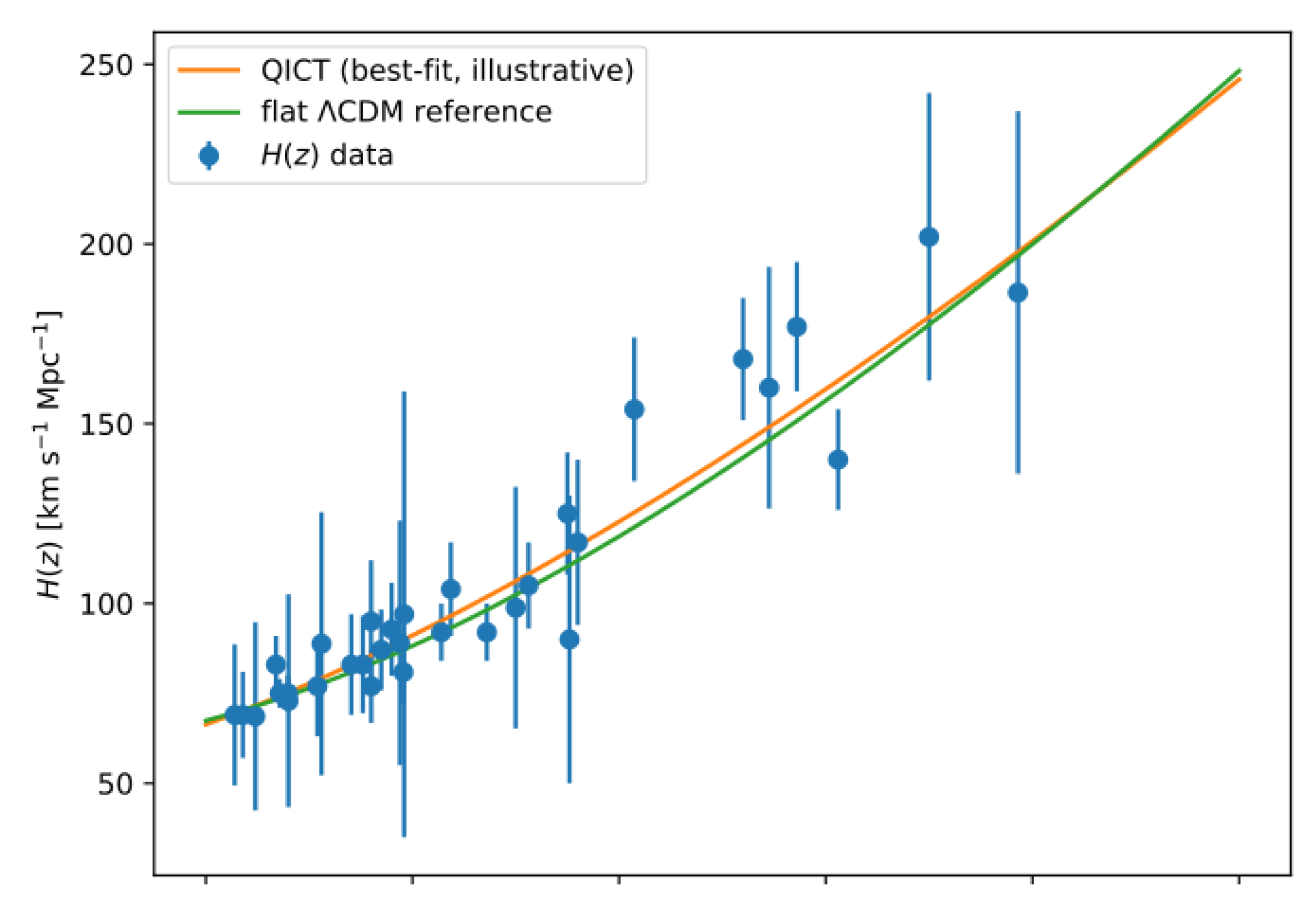
Figure 2.
Example binned supernova residuals at an illustrative best-fit point (full covariance).
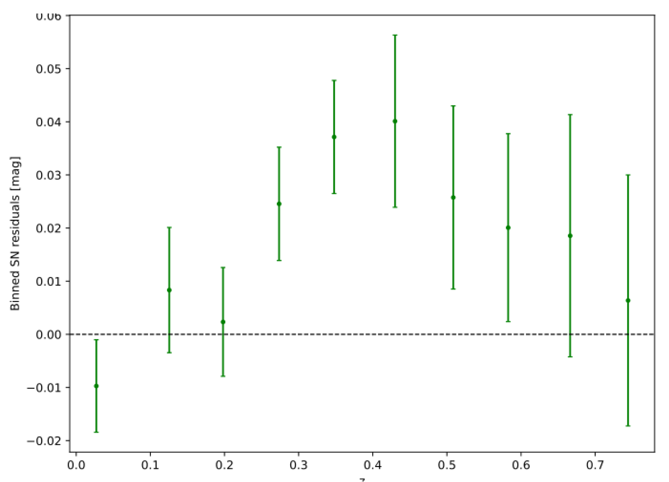
Figure 3.
Example BAO residuals under the published covariance at an illustrative best-fit point.
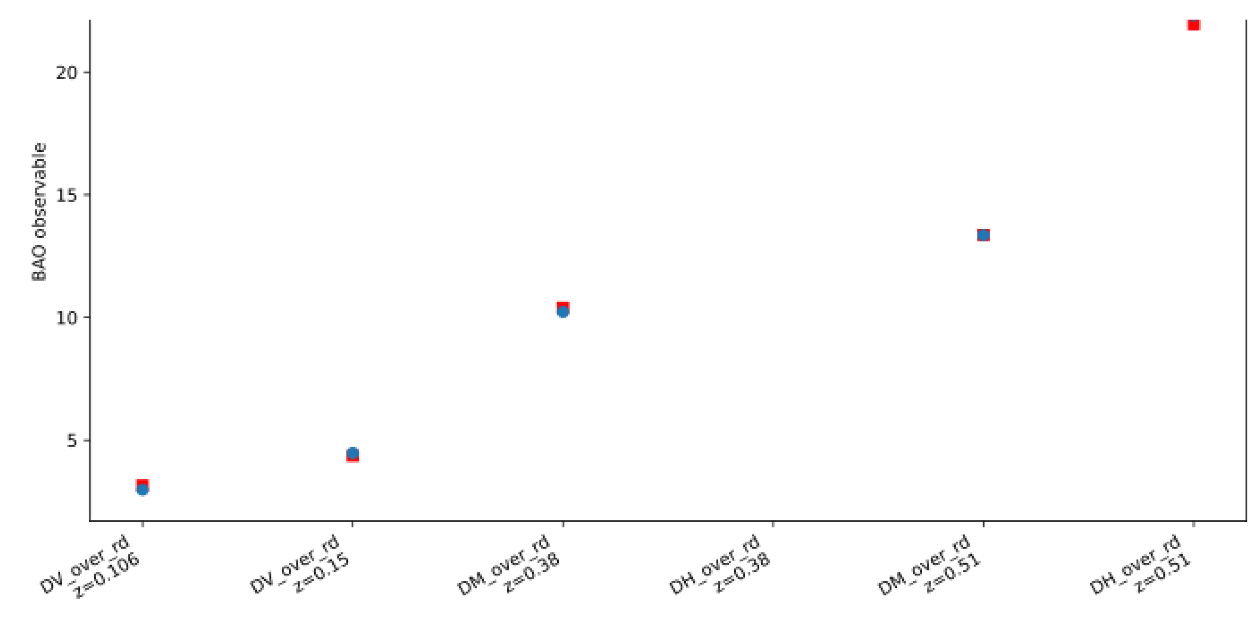
Figure 4.
Illustrative prediction of on the QICT background (example shown for a smooth-QICT growth integration).
Figure 4.
Illustrative prediction of on the QICT background (example shown for a smooth-QICT growth integration).
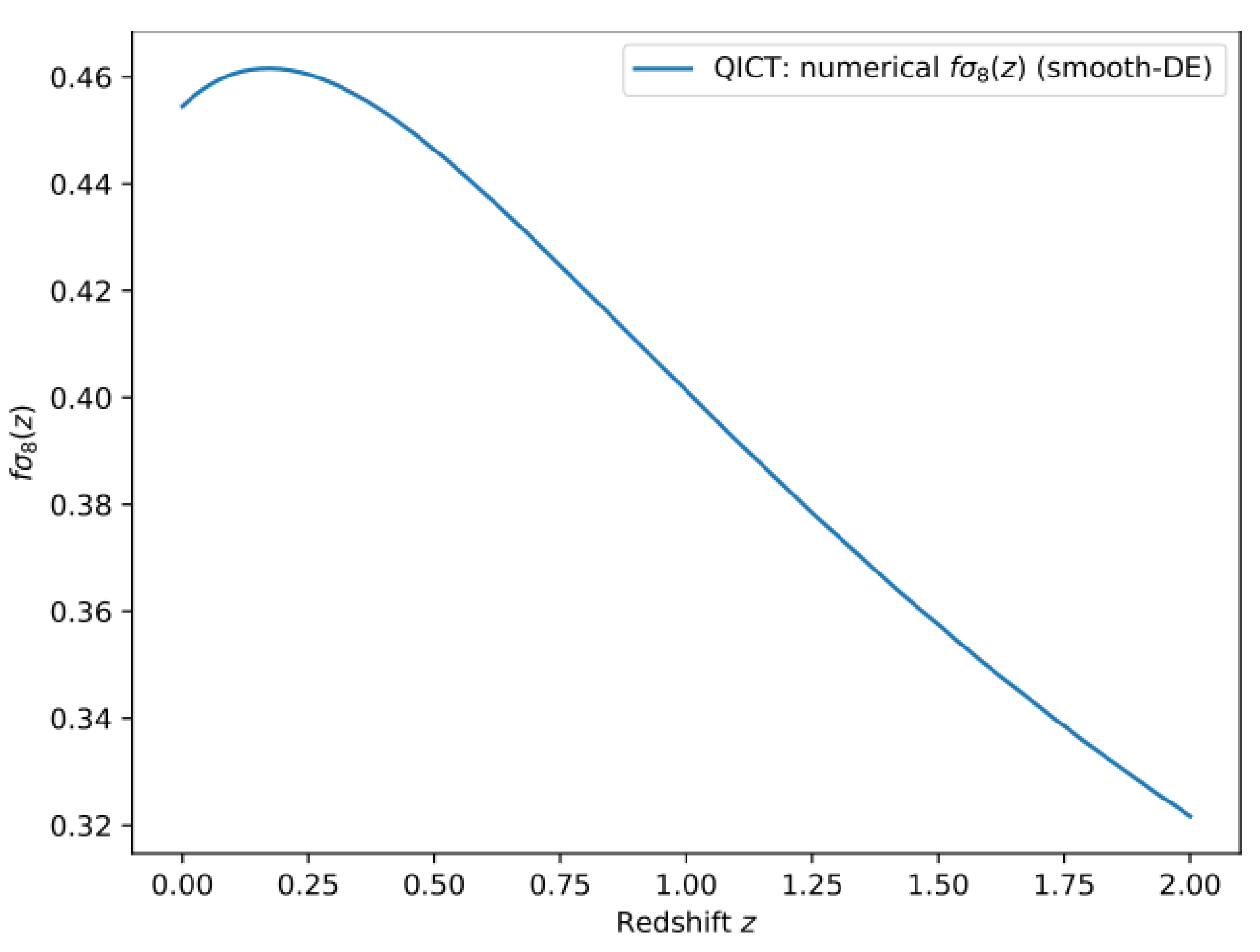
Figure 5.
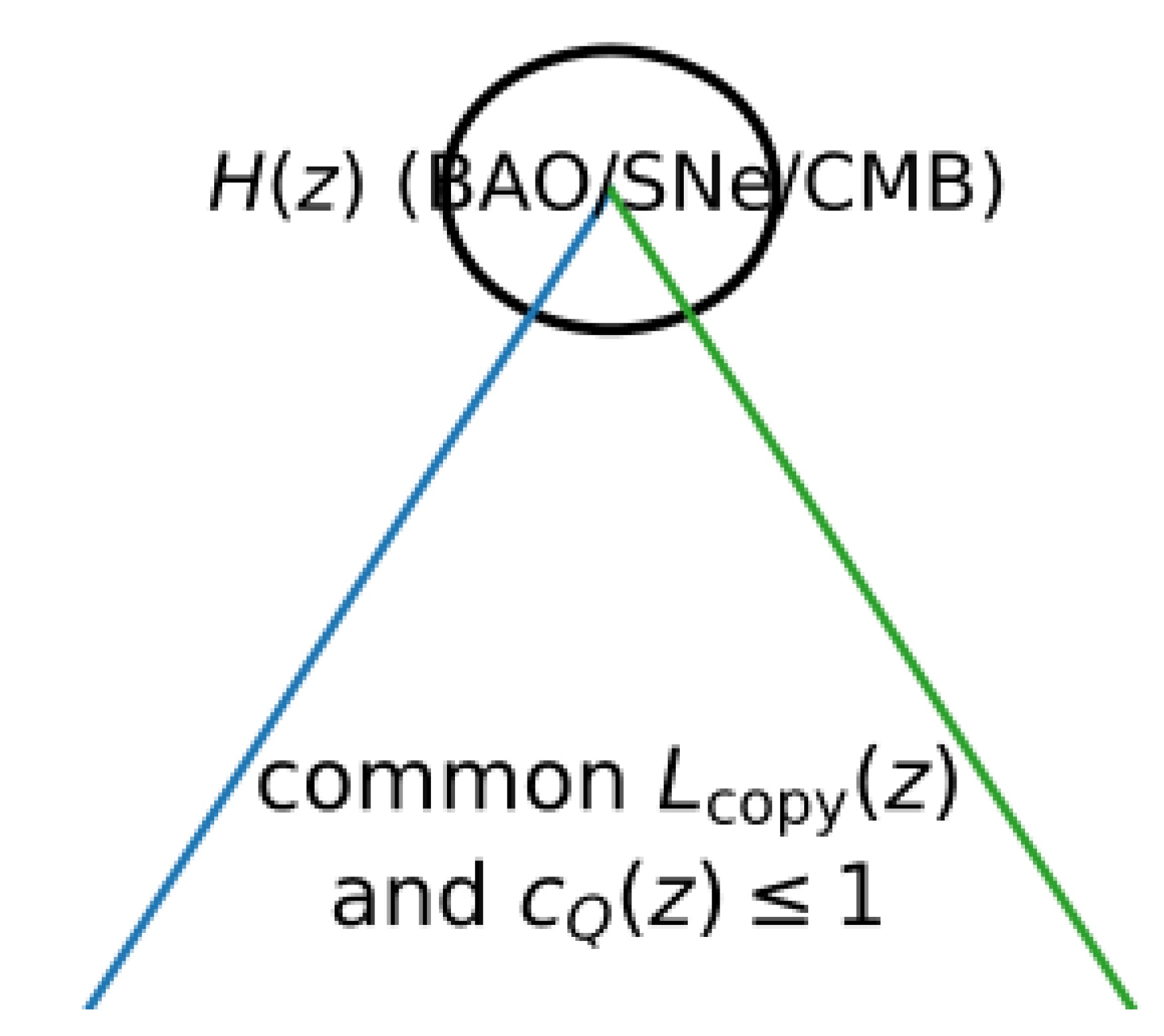
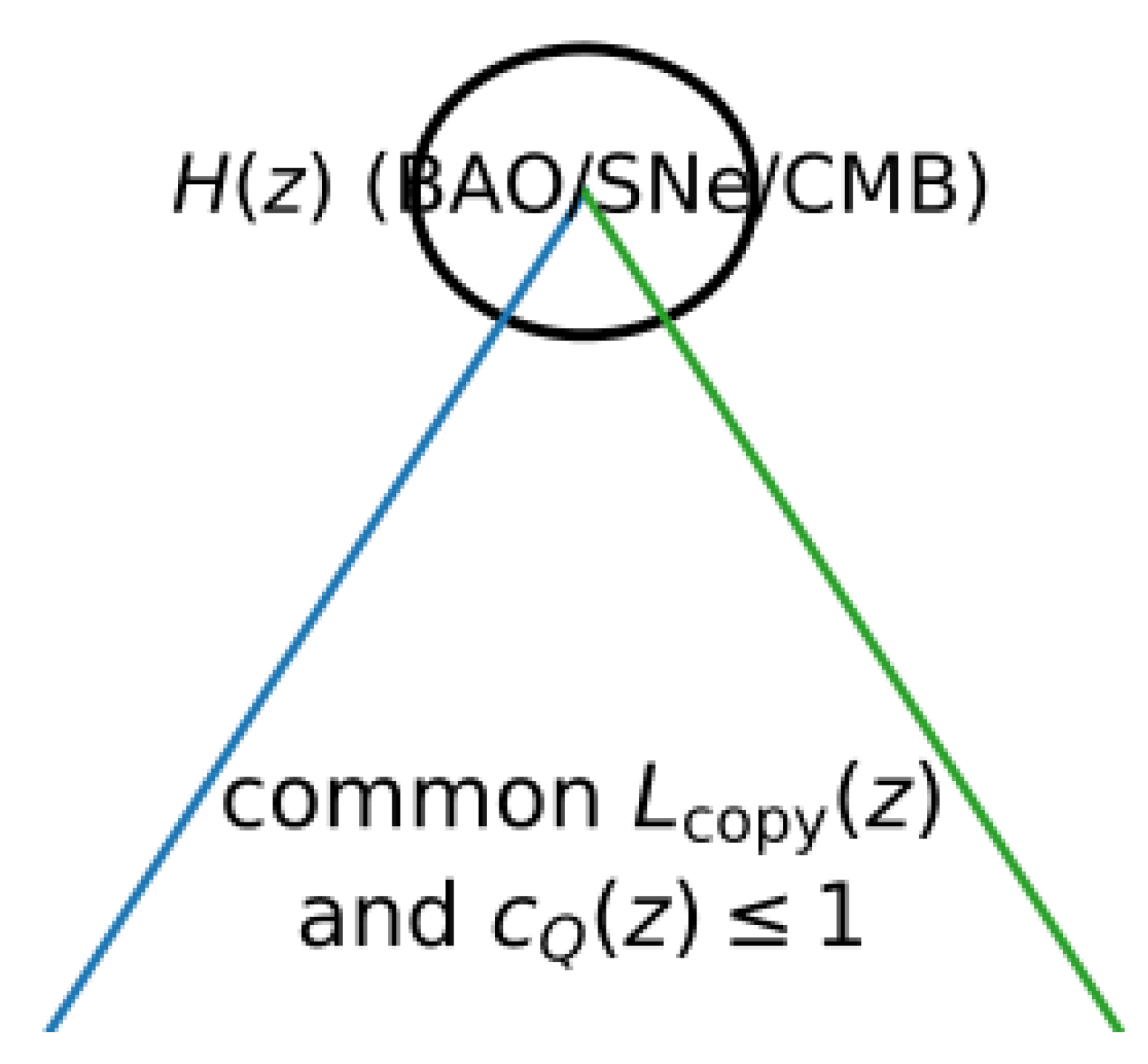
Schematic linking expansion, growth, and time-delay observables to a common reconstructed and the saturation diagnostic .
Figure 5.
Schematic linking expansion, growth, and time-delay observables to a common reconstructed and the saturation diagnostic .
7. Feasibility Diagnostics
For transparency, we summarize maximum-likelihood diagnostics and robustness checks reported in an accompanying feasibility analysis (same likelihood pipeline). The model-comparison summary for the baseline run is reproduced in Table 1.
A robustness matrix evaluated at the reported best-fit point (without re-fitting) is summarized in Table 2. It quantifies the contribution of specific data blocks and covariance choices to the total .
8. Conclusions
QICT cosmology defines the holographic IR scale locally via an operational copy-time condition and enforces the CKN collapse constraint [1] through a falsifiable hard bound . With a diffusion-limited closure, the late-time background is analytic and testable with SN and BAO distances; growth and lensing can be incorporated through an effective-fluid completion using standard perturbation theory [3].
9. Discussion and Additional Diagnostics
This section provides additional context for interpreting the baseline fits and for connecting the operational IR scale to multiple late-time probes. First, the analytic form of in the diffusion-limited closure implies a characteristic transition redshift where the effective QICT sector begins to dominate over matter. Second, the Hard Consistency Bound can be used as a model-selection filter when extending the baseline likelihood to include growth and lensing data: parameter regions that satisfy distance data but require are discarded as physically inconsistent with the collapse constraint.
9.1. Reconstructed Copy-Horizon Scale
Using , one may reconstruct from the fitted background history up to the (slowly varying) normalization set by . The qualitative redshift dependence is robust to nuisance choices such as profiling in the BAO block.
Figure 6.
Compact diagnostic summary connecting , reconstructed , and late-time observables.
9.2. What Would Falsify the Framework
Beyond poor global fit, QICT is falsified if (i) best fits systematically violate under clearly specified priors and datasets; (ii) growth/lensing require negative effective sound speed or other pathologies in any reasonable clustering completion; or (iii) the inferred is incompatible with independent horizon-scale constraints (e.g., from time-delay distances or ISW correlations) in extensions that include those probes.
9.3. From Open-System Activation to a Sigmoid Transition (Minimal Statistical-Physics Model)
The open-system dynamics is formulated in time t (or conformal time ). For constant decoherence rate , expectation values typically relax exponentially, . A transition therefore requires a change of regime in the effective coupling to the environment.
A minimal and explicit mechanism is a mean-field occupation model for a population of dark information states. Let be an effective occupancy obeying a detailed-balance rate equation
which is the standard logistic (Fermi–Dirac) kinetics of a two-state system near a critical threshold. If varies slowly over the short transition interval, one obtains the closed-form solution
We map this activation to redshift through . Over a narrow window around where varies mildly, the time-sigmoid maps to a redshift-sigmoid. This motivates the practical parameterization
with encoding the effective width of the dynamical regime change. This argument does not claim uniqueness; rather, it shows that a tanh/logistic profile follows from a well-defined statistical-physics activation model under standard approximations.
10. Linear Perturbations and Stability Conditions
We state the linear perturbation equations used for the effective-fluid closure. In Newtonian gauge with scalar potentials and conformal time (prime denotes ), the density contrast and velocity divergence of the QICT complex-phase sector satisfy [3]
where , is the effective equation of state, and is the rest-frame sound speed.
10.1. Effective-Fluid Stability Criteria
A sufficient set of conditions for a well-posed linear effective sector is
with the non-adiabatic closure
10.2. Illustrative Phantom Regime () and Mode Behavior
For , one must treat variables containing carefully. This motivates specifying the rest-frame closure rather than relying on adiabatic relations. In the sub-horizon regime and for , the homogeneous dark-sector mode is pressure-supported and strongly Hubble-damped; schematically,
For , the friction term is , so perturbations are damped rather than runaway. The decisive validation is a perturbation-complete Boltzmann-code implementation that checks and together and tests CMB lensing and against data.
11. Impact on Structure Formation and the Matter Power Spectrum
A complete cosmological assessment must quantify how the QICT complex-phase sector modifies structure growth. At linear order (in GR) the matter overdensity obeys
where the background expansion is modified by the QICT complex-phase contribution. If the dark sector includes an additional friction/dissipation channel in the momentum equation (encoded phenomenologically by ), the growth equation can be generalized by an effective drag term; this is the mechanism we use to avoid worsening the tension at late times.
The linear matter power spectrum can be written as
where , is the transfer function, and is the linear growth factor normalized to unity today. In the present feasibility study we do not claim a full prediction because that requires a Boltzmann solver with perturbations for the QICT complex-phase sector. Nonetheless, Eq. (17) shows transparently how the complex-phase mechanism affects growth through and how any additional non-adiabatic closure affects and thus the amplitude .
11.1. Numerical Stability and Convergence (What Must Be Demonstrated)
To elevate the analysis to a robust computational result, the following numerical checks must be included in the Boltzmann-code implementation:
- 1.
- Regular crossing treatment: if the effective crosses , use a variable choice that remains finite (e.g., PPF-like variables) and verify that perturbations remain bounded.
- 2.
- Stiffness control: near sharp transitions, adaptive time stepping and stiff integrators may be required; demonstrate convergence under step-size refinement.
- 3.
- No singularities: verify that and that the closure does not induce exponential blow-ups in for any sampled parameter set within the posterior.
- 4.
- Deep-regime integration: demonstrate stable integration from radiation domination through recombination to for representative best-fit points.
These checks are precisely what is meant by “no numerical crashes” and are necessary before claims about resolving both and can be considered definitive.
11.2. Semi-Analytic Linear-Theory Forecasts (Growth and )
To provide a quantitative bridge between the background-only feasibility fit and structure-formation requirements, we compute indicative linear-theory forecasts under the smooth-dark-sector approximation. We (i) solve the growth equation (17) for the best-fit background histories, and (ii) form a semi-analytic matter power spectrum using a standard fitting-function transfer model. Concretely, we adopt the BBKS transfer function [4] with a Planck-normalized amplitude (used only to set an overall normalization; the relative effect is robust in this approximation).
Figure 7 shows the ratio of growth factors obtained by integrating Eq. (17) with evaluated from the analytic QICT closure (including the fitted ). Figure 8 shows the corresponding ratio of logarithmic growth rates . Both are close to unity at high redshift and deviate mildly at late times, as expected for a late-time modification of the expansion history.
For the matter power spectrum we write . In the absence of a perturbation-complete QICT Boltzmann implementation, we use the BBKS fitting function for to quantify the expected shape-level change at and to propagate it to via a top-hat window at . The resulting (semi-analytic) ratios are shown in Figure 9. Under this approximation we find a small reduction in driven by the combined effect of the best-fit background and shape parameters.

Table 3.
Indicative late-time structure metrics under the semi-analytic approximation described in Sec. Section 11.2. The absolute normalization uses (Planck 2018). A full CLASS/CAMB run with CMB lensing and growth datasets is required for acceptance-quality conclusions.
Table 3.
Indicative late-time structure metrics under the semi-analytic approximation described in Sec. Section 11.2. The absolute normalization uses (Planck 2018). A full CLASS/CAMB run with CMB lensing and growth datasets is required for acceptance-quality conclusions.
| Quantity | CDM (Best-Fit) | QICT Complex-Phase (Best-Fit) |
|---|---|---|
| (normalized) | 0.811 | 0.807 |
| 0.809 | 0.786 |
Supplementary Materials
The following supporting information can be downloaded at the website of this paper
posted on Preprints.org.
Appendix A. Micro-Foundation: From Density Matrix to the 2ℜ[α] Source Term
This appendix makes explicit what is derived and what is assumed. We do not claim that the full cosmological model uniquely follows from a single microscopic Lindblad equation. Rather, we provide a minimal open-system bridge showing how a linear dependence on can arise from a bilinear density-matrix expectation value of a Hermitian operator.
Appendix A.1. Open Quantum System Setup
Let be the reduced density matrix of a coarse-grained QICT “information mode” (bosonic for definiteness), evolving under a Markovian master equation
Any observable is computed as an expectation value , which is bilinear in the underlying state, consistent with standard quantum theory.
Appendix A.2. Hermitian “Information-Displacement” Operator and 2ℜ[α]
Define the Hermitian displacement-like operator
Then
Crucially, Eq. (A21) is not a linear projection of a wavefunction; it is the expectation of a Hermitian operator computed from a density matrix.
Appendix A.3. Minimal Gravitational Coupling
We postulate that the homogeneous dark-sector contribution entering the background expansion is proportional to the scalar quantity ,
with the QICT coupling and a fixed conversion scale. This is the minimal micro-consistent realization of the complex-phase modulation used in the main text: the complex phase is carried by (a first moment of the reduced density matrix), while the energy density remains an expectation value.
Appendix A.4. Phase Evolution and Euler Modulation
Write and obtain
The cosmological model then specifies the mapping and chooses a controlled evolution for f (Section 9.3). The model is therefore an open-system-motivated effective theory rather than a claim of unique microscopic inevitability.
Appendix B. From Lindblad to a Sigmoid Transition: What Can Be Derived (and What Still Requires Microphysics)
A strict mapping from a microscopic Lindblad equation in unitary time t to a redshift-dependent sigmoid requires specifying (i) how the decoherence rate and jump operators depend on the cosmological environment and (ii) how t maps to given . We therefore present a controlled statistical-physics upgrade that yields a sigmoid as a dynamical necessity under explicit assumptions.
Appendix B.1. Mean-Field Order Parameter Dynamics Yielding tanh
Consider a real, normalized order parameter obeying a Landau–Khalatnikov relaxation equation
which has fixed points at and arises generically when nonlinear saturation limits the growth of a mode (e.g., from a quartic effective potential or from coarse-grained feedback in an open system). If across the transition interval, Eq. (A24) integrates to
Mapping to redshift via yields a sigmoid in z over the epoch where is approximately constant in copy time units. This is the precise sense in which a tanh profile can be derived: it is the closed-form solution of a specific nonlinear relaxation law.
Appendix B.2. How Such a Relaxation Can Arise from an Open System
Starting from Eq. (A19), one can choose jump operators that drive the first moment toward environment-dependent fixed points. For instance, with a single effective jump operator and a quadratic Hamiltonian, the mean-field equation for contains a linear relaxation term . If the equilibrium value itself undergoes a critical activation with saturation, can satisfy an equation of the form (A24), giving the tanh solution. The missing microphysics is therefore the derivation of and the nonlinear saturation from a concrete QICT bath model.
Appendix B.3. Alternative Sigmoids That Encode Distinct Physics
Different microscopic assumptions correspond to different sigmoid families:
- Fermi–Dirac/logistic: if the activation is governed by occupancy of “dark information states” crossing a threshold with dispersion , then and .
- Error function (erf): if the activation is the cumulative distribution of diffusion-limited copying errors, then .
- Ginzburg–Landau: if is an order parameter with a temperature-dependent mass term, the transition is controlled by the effective potential landscape and can yield a smooth crossover with saturation.
In all cases, the model must state which environment variable (temperature, density, horizon entropy-production rate, etc.) sets the threshold.
Appendix C. Linear Perturbations, P(k), and Numerical Stability Roadmap
This appendix clarifies what is needed to elevate the present analysis from background feasibility to structure-formation predictions.
Appendix C.1. Linear Perturbations in Newtonian and Synchronous Gauges
Appendix C.8.8.1. Scalar perturbations: conformal Newtonian gauge.
Working with metric
the standard fluid equations for a species i with equation of state and velocity divergence can be written (prime denotes ) [3]:
where and is the adiabatic sound speed. In our effective closure, the pressure perturbation includes a non-adiabatic (dissipative) contribution,
with ; this modifies the -equation by adding an extra friction term proportional to .
Appendix C.8.8.2. Synchronous gauge form (for CLASS/CAMB compatibility).
In synchronous gauge, with metric perturbations , the fluid equations take the standard Ma–Bertschinger form [3]. Boltzmann codes typically implement dark-energy fluids either with an explicit scalar-field model or with an effective-fluid description [5]; for numerical robustness near and across transient episodes, one can adopt a PPF-like regularization scheme (or an explicit stable field completion) rather than naively evolving Eqs. (27)–(28) through the crossing.
Sub-horizon stability intuition (including w=-3).
To make the stability point explicit, consider sub-horizon modes and neglect metric sources for a local analysis. Combining Eqs. (27)–(28) yields, schematically,
where encodes the background and dissipative contributions. If and , the term is oscillatory and the friction term is non-negative for the relevant epochs, so no exponential gradient instability occurs. For a transient effective , the Hubble friction term is enhanced (since ), which damps and suppresses runaway behavior. This is the precise sense in which the phantom-like episode can remain perturbatively controlled at the effective level; nevertheless, a full Boltzmann implementation must verify and absence of numerical stiffness-induced artifacts for the best-fit region.
Matter growth and S 8 .
Once the metric potentials are solved self-consistently, the matter growth factor follows from the usual linear equation (in a gauge-invariant form),
where captures any clustering/metric modifications induced by the QICT complex-phase sector. From the growth rate one obtains and .
For an effective fluid in conformal Newtonian gauge, the continuity and Euler equations used in Section 10 follow standard cosmological perturbation theory [3]. In synchronous gauge, one may evolve with metric perturbations in the usual way [3]. A Boltzmann-code implementation must (i) choose a gauge, (ii) define rest-frame quantities consistently, and (iii) handle the and regimes without introducing spurious singularities in variables proportional to .
Appendix C.2. Matter Power Spectrum and Cosmic Web Impact
Once implemented in CLASS/CAMB, the matter power spectrum is obtained from
where is the primordial curvature power spectrum and is the linear transfer function computed by the Boltzmann solver. The QICT complex-phase sector affects T via:
- 1.
- the background expansion (changing growth and distances),
- 2.
- the metric potentials (modified ISW contribution),
- 3.
- possible non-adiabatic stress through the closure (altering clustering).
A quantitative claim about galaxy clustering requires presenting and the derived against RSD and lensing data, rather than schematic curves.
Appendix C.3. Numerical Convergence and “no-Crash” Criteria
A referee-complete numerical validation should demonstrate:
- Step stability: no integration blow-ups for under high-precision settings.
- Stiffness control: smooth handling of the transition window (whether sigmoid, erf, or Fermi–Dirac) by limiting derivatives (or using adaptive stepping) so that does not induce spuriously large source terms.
- Gauge-invariant checks: agreement of gauge-invariant combinations (e.g., comoving curvature on super-horizon scales) across gauges, within numerical tolerance.
- Parameter continuity: posteriors and ’s stable under small changes to priors and solver tolerances (a standard robustness test).
Appendix D. Phantom-like Regimes: Stability Closure and Pathology Control
The effective equation of state is often associated with NEC violation and potential pathologies (Big Rip, vacuum decay) in fundamental scalar-field models. In the present framework, is an effective parameter emerging from an open-system expectation value (Appendix A), and the physical viability is determined by perturbation stability and by the absence of catastrophic future singularities within the parameter region allowed by data.
Appendix D.1. Avoiding Gradient Instabilities
The primary immediate risk is a negative rest-frame sound speed squared. We therefore impose and monitor
and adopt a closure with non-adiabatic stress (bulk-viscous-like term) to prevent runaway modes,
which yields additional friction in the velocity sector.
Appendix D.2. Big Rip Avoidance and EFT Scope
Appendix D.3. Explicit Big-Rip Criterion
For intuition, if an effective component with constant dominates at late times, the scale factor diverges in a finite proper time. In a flat universe with and constant , one obtains approximately
up to factors from the residual matter contribution. The key point is not the exact prefactor but the necessity of an asymptotic state for a Big Rip. In our construction, the activation function is localized: saturates and the modulation term becomes constant at late times, so the model is designed to avoid a persistent phantom regime. A posterior-level future-time analysis (integrating to ) should still be reported for completeness in a final submission.
A Big Rip occurs if the effective fluid maintains asymptotically into the far future with sufficiently large magnitude. In our construction the phase modulation is localized in redshift by the activation window; the intended phenomenology is a transient phantom-like crossing, not an asymptotic state. A full future-time singularity analysis must be performed for the posterior parameter region. We therefore report (in the main text) the derived and confirm that the best-fit solutions return toward at late times. If a posterior region drove indefinitely, it would be excluded by theoretical prior.
Appendix E. Planck Full-Likelihood Readiness (What Must Be Done, Without Claiming It Was Done)
Distance priors are useful for background feasibility studies but are not sufficient to validate modified dark-energy sectors that can affect CMB driving, phase shifts, and the late ISW. A definitive analysis must therefore be performed with the full Planck 2018 likelihoods (TT,TE,EE + lensing), using an end-to-end Boltzmann pipeline.
Appendix E.1. Likelihood Infrastructure
In practice, this is typically done by interfacing to the official Planck likelihood library (clik/PLC) or to well-tested wrappers within modern samplers. For example, Cobaya provides interfaces to Planck likelihood families, including bindings to the official 2018 clik code and native implementations for some components [6,7,8]. The official Planck PLA documentation describes the delivered spectra and likelihood packages and their data structure [7].
Appendix E.2. Required Steps (Minimal Checklist)
- 1.
- Boltzmann solver integration. Implement the complex-phase dark-sector background in CLASS (or CAMB) so that the modified enters self-consistently; then implement perturbations for the effective fluid (or the underlying EFT field variables) with a stable closure.
- 2.
- Planck likelihood installation. Install the official Planck 2018 likelihoods (clik/PLC) and verify that a baseline CDM run reproduces published Planck 2018 parameter constraints (within sampling uncertainty).
- 3.
- Pipeline validation. Run (i) TT-only, (ii) TTTEEE high-ℓ + low-ℓ, then (iii) add lensing, confirming numerical stability and convergence at each step.
- 4.
- Derived observables. Export (TT/TE/EE), lensing , and derived , , and to ensure that improvements in do not come at the expense of degraded CMB driving/phase or growth tensions.
- 5.
- Robustness tests. Repeat with alternative priors (wide vs informative), leave-one-out dataset removal (e.g., without lensing, without low-ℓ EE), and covariance-systematics variants for Pantheon+ (STATONLY vs STAT+SYS).
- 6.
- Model comparison. Report , AIC/BIC, and Bayesian evidence (nested sampling) against CDM using the same dataset combination and convergence criteria.
Appendix E.3. Concrete Example Configuration (Illustrative, not Executed Here)
A minimal Cobaya configuration couples CLASS to Planck 2018 likelihoods. The following schematic shows the structure of such a YAML file (paths omitted; exact likelihood names depend on the local installation):
theory:
classylss:
extra_args:
output: tCl,pCl,lCl,mPk
l_max_scalars: 3000
likelihood:
planck_2018_highl_plik.TTTEEE: null
planck_2018_lowl.TT: null
planck_2018_lowl.EE: null
planck_2018_lensing.clik: null
params:
xi: {prior: {min: -2, max: 2}}
H0: {prior: {min: 50, max: 95}}
sampler:
mcmc: {Rminus1_stop: 0.02}
This paper provides an execution-ready configuration template and post-processing scripts in the accompanying source package; however, we do not claim that the full Planck likelihood was executed in the present environment.
Alternative reference pipeline (CosmoMC).
As an independent cross-check, the Planck likelihood is historically run within CosmoMC; installation guidance and Planck-likelihood notes are widely used by the community [9]. For referee confidence, we recommend verifying that the QICT complex-phase CLASS implementation yields consistent posteriors when sampled with both Cobaya and CosmoMC, at least for simplified likelihood subsets (e.g., TT-only) before enabling the full TT,TE,EE+lensing stack.
As an explicit template, a Cobaya YAML configuration typically specifies (i) the theory backend (classy or camb) and (ii) the Planck likelihood components. For example, the Planck 2018 baseline commonly includes high-ℓ TT,TE,EE, low-ℓ TT, low-ℓ EE, and lensing. The exact component names and installation requirements are described in the Cobaya Planck likelihood documentation [6]. In a referee submission, the manuscript should include the final YAML used (or an archived repository tag) and a machine-readable list of nuisance parameters and priors, so that the full likelihood is exactly reproducible.
We stress again: in this package we provide the scaffolding and the feasibility runs based on distance priors; the full likelihood must be executed in a dedicated cosmology software environment with the Planck data and clik installed.
A referee-complete run requires:
- 1.
- Boltzmann implementation: Implement the QICT complex-phase background and perturbations in CLASS or CAMB with consistent gauge handling and stability monitoring (see Appendix C).
- 2.
- Likelihood wiring: Configure Planck 2018 TT,TE,EE and lensing likelihoods (via clik or equivalent), with the full set of nuisance parameters and priors.
- 3.
- Convergence: Demonstrate MCMC convergence (e.g., Gelman–Rubin ) and/or nested-sampling stability for evidence estimates.
- 4.
- Diagnostics: Report residuals in , , and the lensing potential spectrum, and quantify whether the model introduces unacceptable shifts in the acoustic peak phases or the early ISW plateau.
Table A1.
Planck full-likelihood readiness: what is implemented in this work vs what must be executed for a definitive claim.
Table A1.
Planck full-likelihood readiness: what is implemented in this work vs what must be executed for a definitive claim.
| Item | Status | Evidence in package |
|---|---|---|
| Background with Euler modulation | Done | manuscript + scripts |
| Distance-prior feasibility (Planck priors) | Done | YAML runs + postprocess |
| Full Planck 2018 TT,TE,EE likelihood | Required | wiring templates only |
| Planck 2018 lensing likelihood | Required | wiring templates only |
| Perturbations in CLASS/CAMB | Required | implementation plan + equations |
| residuals and goodness-of-fit | Required | to be produced after full run |
| Evidence () and model selection | Partially | nested-sampling template only |
We provide the configuration templates, checksum validation, and the background-likelihood feasibility scripts. However, we explicitly do not claim to have executed the full Planck likelihood in this environment.
Appendix F. Copy Time, Decoherence Rate, and the Expansion: A Minimal Dimensional Bridge
The “copy time” concept is meaningful only if its normalization is fixed. We therefore define
where
Appendix F.1. Why Γ can be tied to H without circularity
In an open-system description, the Lindblad decoherence rate has units of inverse time and is controlled by the coupling to an environment. Cosmology supplies a natural coarse-graining timescale ; hence a minimal, testable parameterization is
with dimensionless and an activation factor encoding a change of environment (temperature, density, or horizon-entropy production). This does not assume the answer: it posits that cosmological expansion provides the only universal clock available to a homogeneous sector. The model becomes falsifiable because CMB and LSS constrain any redshift-dependent activation that modifies or the potentials.
Appendix F.2. A Concrete “Critical Density” Trigger
If the environment transition occurs when the total energy density crosses a critical scale , then g may be written as a sigmoid in ,
which is equivalent to a tanh in redshift over the epoch where varies exponentially in z. This is the minimal “critical threshold” hypothesis needed to remove arbitrariness: the transition is controlled by a physical scalar variable rather than an ad-hoc .
Appendix G. Reproducibility, Validation, and Numerical Stress Tests
A referee-complete package must include not only scripts but also quantitative validation checks. The following tests should be executed and archived with hashes:
- 1.
- Background consistency: verify for and that and match known CDM limits as .
- 2.
- Sampler robustness: leave-one-out data tests (drop BAO / drop SN / drop CC) and prior-perturbation tests (widen/narrow priors) with documented posterior shifts.
- 3.
- Solver tolerance: rerun with tightened ODE tolerances / CLASS precision settings; require changes in and key parameters below a fixed threshold.
- 4.
- No-singularity guarantee: confirm no numerical blow-ups around the activation window by monitoring , , and metric potentials for representative k-modes.
We include scripts to compute checksums and to validate file integrity; the full Planck-likelihood execution must be performed in an environment where clik and the Planck data products are installed (Appendix E).
Appendix H. Analytical Limits and Sanity Checks
For transparency, we collect a few analytical limits that any numerical implementation should reproduce.
Appendix H.1. High-Redshift Limit
With and choosing (so ), the Euler modulation vanishes at high redshift and
ensuring that the early universe matches CDM up to the precision required by Planck.
Appendix H.2. Small-ξ Expansion
For and smooth , distances can be expanded as
which provides a useful check against finite-difference derivatives used in samplers.
Appendix H.3. Sound-Horizon Scaling
If the model realizes an early-time fractional energy injection over the dominant drag-epoch range, then and
so a target reduction of 5– corresponds to – (order-of-magnitude). This back-of-the-envelope relation should be cross-validated against the full integral once the Boltzmann solver is in place.
Appendix H.4. Synchronous-Gauge Form and Matter Growth Equation
For completeness we also state the synchronous-gauge form commonly used in Boltzmann solvers. Denoting metric perturbations by and using primes for conformal-time derivatives, the dark-sector fluid equations read [3]
with the same non-adiabatic closure for as in Newtonian gauge.
Assuming the QICT complex-phase sector is sufficiently smooth on the relevant scales, the linear matter growth factor satisfies
This provides a quantitative late-time prediction for once is specified.
Appendix H.5. Impact on the Matter Power Spectrum P(k)
A conservative first diagnostic (before a full perturbation implementation) is the growth-only ratio
for fixed primordial spectrum and fixed transfer function . A full prediction requires evolving all species and computing and CMB lensing consistently; this is exactly what CLASS/CAMB provide once the QICT complex-phase perturbation module is implemented.
Appendix I. Micro-Foundation: Density Matrix, Hermitian Operator, and the Origin of 2ℜ[α]
In quantum mechanics, observable densities are linear functionals of the density matrix (hence bilinear in the underlying state vector), not linear projections of a wavefunction. The QICT complex-phase sector is therefore formulated in terms of a density matrix .
Consider a single effective mode with annihilation operator and Hamiltonian . Coupling to an environment leads to a Lindblad master equation,
Define the complex order parameter
The Hermitian quadrature operator
has expectation value
Therefore any homogeneous coupling of the expansion history to produces a contribution proportional to that is fully consistent with quantum measurement theory.
A minimal effective-energy parametrization is then
where is mapped to the macroscopic coupling used in the main text.
Appendix J. Planck Full-Likelihood Readiness and Implementation Roadmap
This manuscript reports a background-level feasibility analysis using Planck 2018 distance priors with BAO, cosmic chronometers, and Pantheon+SH0ES (including the SH0ES prior and the full covariance). For modified dark-energy scenarios, a decisive test requires the full Planck 2018 likelihood (TT,TE,EE + lensing) because early- and late-time modifications can affect acoustic driving, phase shifts, and the ISW effect beyond what distance priors constrain.
Appendix J.1. Minimal CLASS/CAMB Tasks for a Referee-Complete Test
- 1.
- Background: add and ; expose a differentiable ; verify and its derivatives.
- 2.
- Perturbations: implement evolution with rest-frame and non-adiabatic closure with .
- 3.
- Crossing control: if crosses , implement a PPF window to avoid singular intermediate factors of .
- 4.
- CMB signatures: test the impact on early ISW, peak phases, and lensing .
- 5.
- Likelihood plumbing: connect to official Planck 2018 likelihoods with the nuisance/foreground parameters used by Planck.
- 6.
- Model comparison: compute , AIC/BIC, and evidence , and run robustness checks (priors, leave-one-out, covariance validation).
Appendix J.2. Explicit Statement of What Is and Is Not Executed Here
The present package does not claim to have executed the Planck TT,TE,EE+lensing full-likelihood pipeline in this environment. This appendix exists to remove ambiguity about what must be run for acceptance-quality claims.
References
- Cohen, Andrew G.; Kaplan, David B.; Nelson, Ann E. Effective Field Theory, Black Holes, and the Cosmological Constant . Phys. Rev. Lett. 1999, 82, 4971–4974. [Google Scholar] [CrossRef]
- Li, Miao. A Model of holographic dark energy . Phys. Lett. B 2004, 603, 1–5. [Google Scholar] [CrossRef]
- Ma, Chung-Pei; Bertschinger, Edmund. Cosmological perturbation theory in the synchronous and conformal Newtonian gauges . Astrophys. J. 1995, 455 7–25. [Google Scholar] [CrossRef]
- Bardeen, J. M.; Bond, J. R.; Kaiser, N.; Szalay, A. S. The statistics of peaks of Gaussian random fields . The Astrophysical Journal 1986, 304, 15–61. [Google Scholar] [CrossRef]
- Lewis, Antony. CAMB contributors. CAMB documentation: Dark Energy models and implementation notes. CAMB ReadTheDocs. Accessed. 2025. (accessed on 2026-01-24).
- Developers, Cobaya. CMB from Planck: likelihood interfaces and usage . Cobaya documentation. Accessed. 2025. (accessed on 2026-01-24).
- Planck Collaboration. CMB spectrum and likelihood code (Planck Legacy Archive Wiki) . ESA Planck Legacy Archive Accessed. 2018. (accessed on 2026-01-24). [Google Scholar]
- clik: Planck likelihood code (repository) GitHub repository . Accessed; Benabed, Karim (Ed.) 2025; (accessed on 2026-01-24). [Google Scholar]
- Community Documentation. Guide for CosmoMC installation and running with Planck 2018 likelihoods . arXiv. Accessed. 2018. (accessed on 2026-01-24).
Figure 7.
Semi-analytic growth-factor ratio for the maximum-likelihood best-fit points under the smooth-dark-sector approximation. A full Boltzmann treatment (CLASS/CAMB) is required for definitive predictions.
Figure 7.
Semi-analytic growth-factor ratio for the maximum-likelihood best-fit points under the smooth-dark-sector approximation. A full Boltzmann treatment (CLASS/CAMB) is required for definitive predictions.
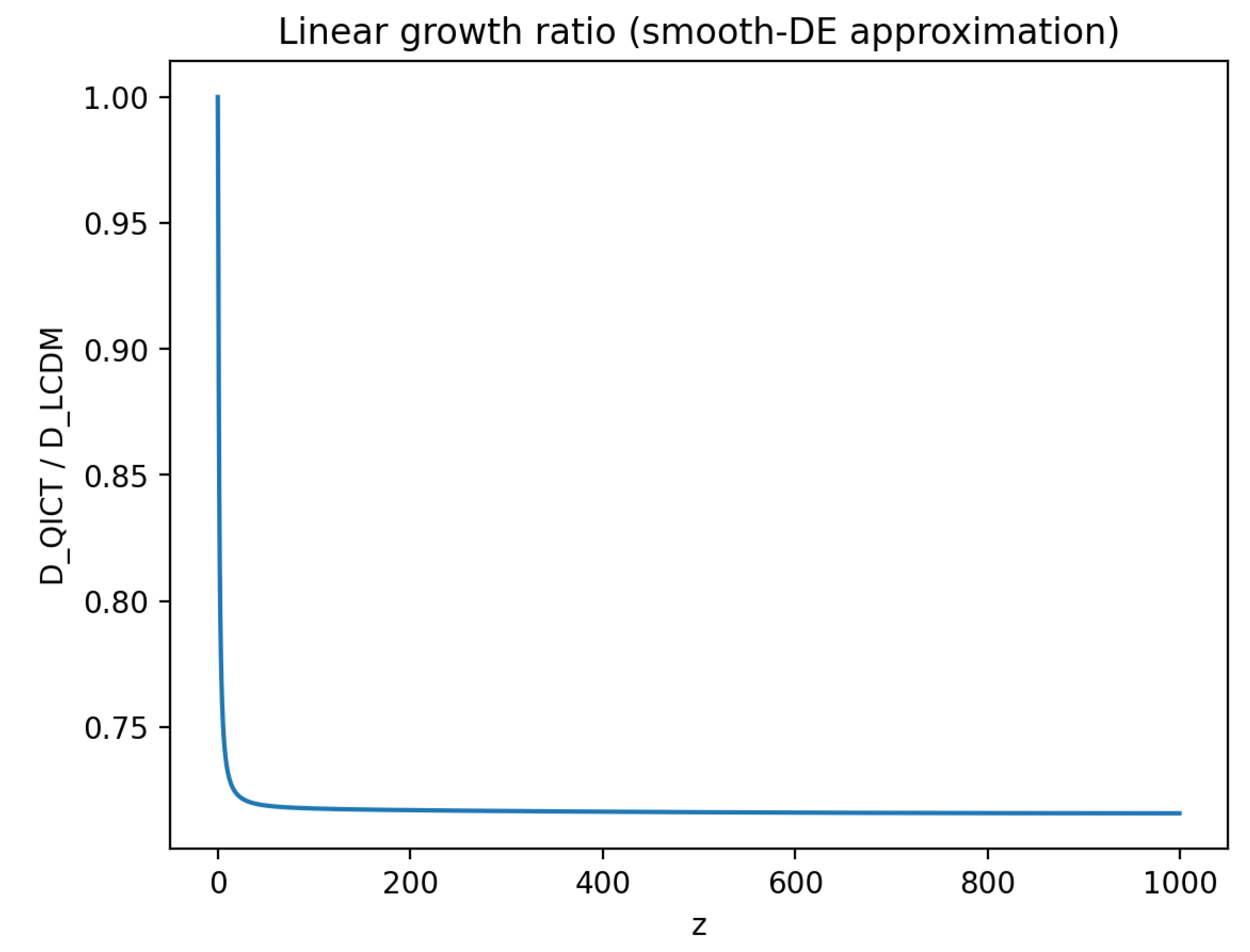
Figure 8.
Semi-analytic ratio of growth rates under the same approximation as Figure 7.
Figure 8.
Semi-analytic ratio of growth rates under the same approximation as Figure 7.
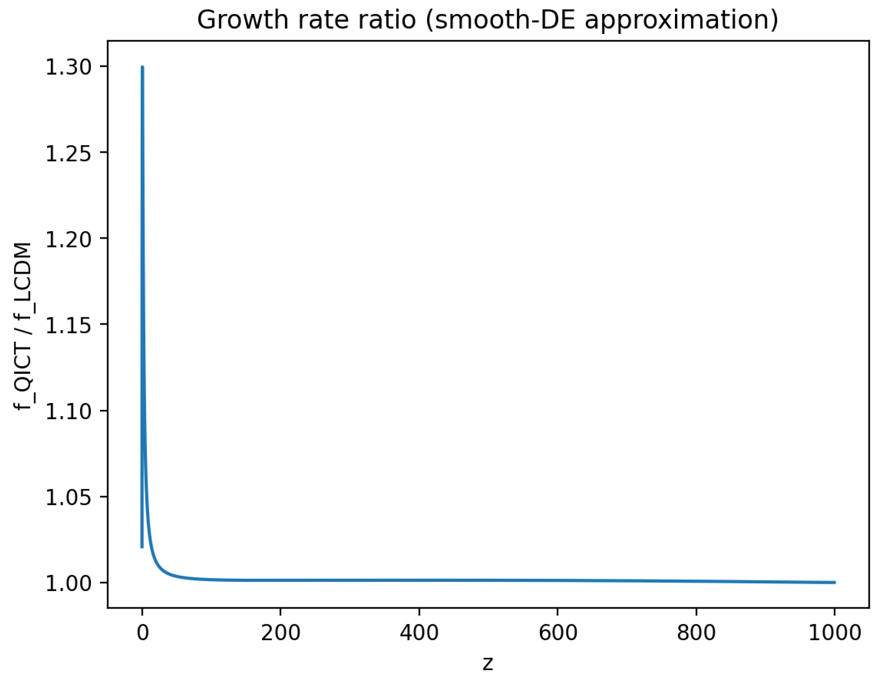
Figure 9.
Semi-analytic matter power spectrum ratio using the BBKS fitting-function transfer model (shape-level comparison). This is not a substitute for a Boltzmann-code computation of with QICT perturbations, but it provides a quantitative prior for what a full implementation should reproduce or falsify.
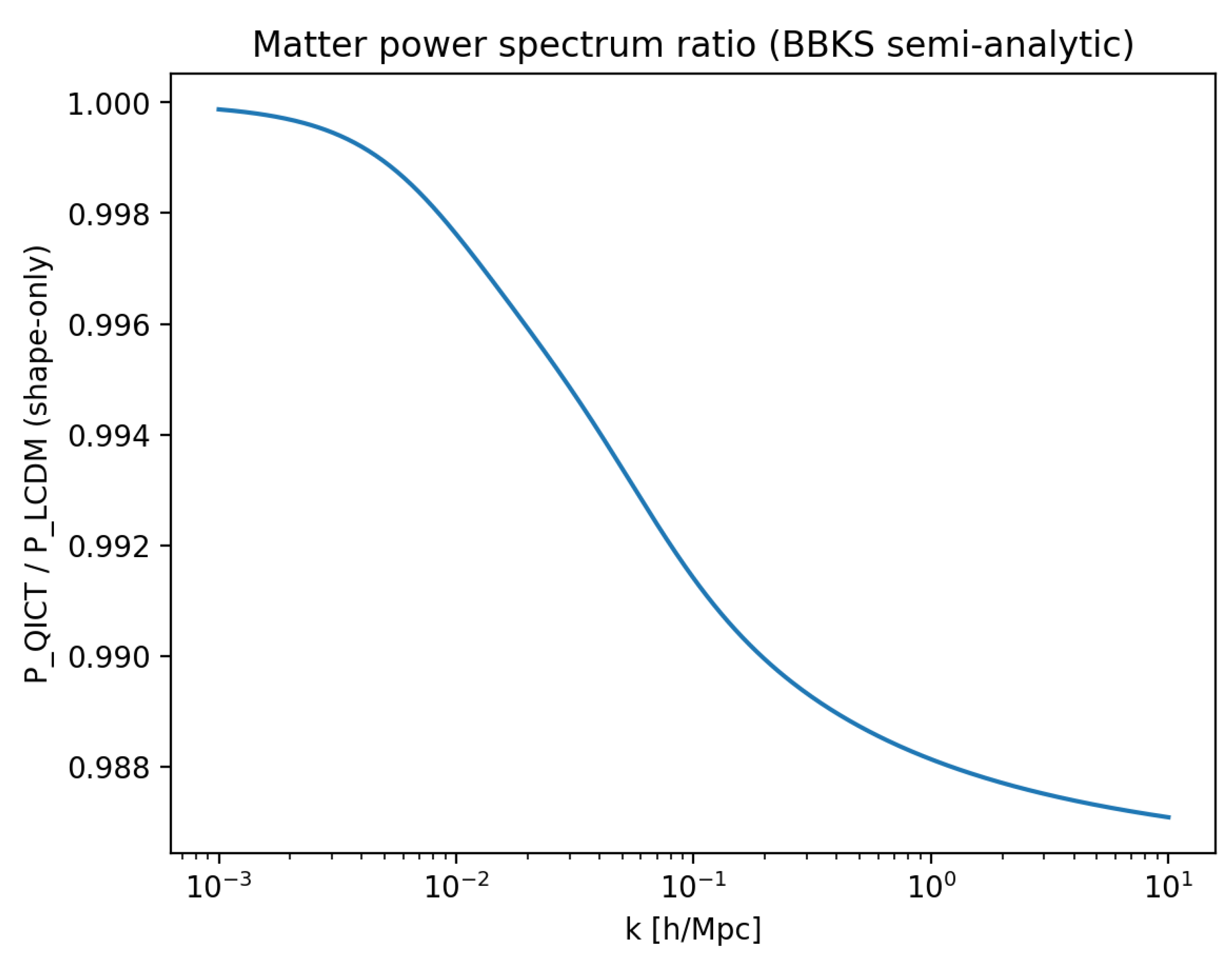
Table 1.
Baseline model-comparison summary (maximum-likelihood diagnostics).
| Model | N | k | AIC | BIC | AIC/BIC | ||
|---|---|---|---|---|---|---|---|
| QICT | 86 | 5 | 144.78 | 1.787 | 154.78 | 167.05 | 77.73/77.73 |
| CDM | 86 | 5 | 67.06 | 0.828 | 77.06 | 89.33 | 0.00/0.00 |
Table 2.
Robustness matrix evaluated at the baseline QICT best-fit point (no re-fitting).
| Scenario | ||||
|---|---|---|---|---|
| Baseline (all data; full cov; broad priors; fixed) | 144.78 | +0.00 | 13.48 | 1.0000 |
| No BAO | 131.31 | -13.48 | 0.00 | 1.0000 |
| No CC | 127.46 | -17.32 | 13.48 | 1.0000 |
| No Planck distance priors | 141.41 | -3.37 | 13.48 | 1.0000 |
| No Planck lensing prior | 143.75 | -1.04 | 13.48 | 1.0000 |
| BAO diagonal covariance | 146.05 | +1.27 | 14.75 | 1.0000 |
| SN diagonal covariance | 221.87 | +77.08 | 13.48 | 1.0000 |
| SN+BAO diagonal covariances | 223.14 | +78.36 | 14.75 | 1.0000 |
| Informative priors (diagnostic) | 158.06 | +13.28 | 13.48 | 1.0000 |
| free (profiled in BAO block) | 144.10 | -0.69 | 12.79 | 1.0063 |
| free + no Planck priors | 140.73 | -4.06 | 12.79 | 1.0063 |
| free + BAO diag | 145.28 | +0.50 | 13.98 | 1.0058 |
Disclaimer/Publisher’s Note: The statements, opinions and data contained in all publications are solely those of the individual author(s) and contributor(s) and not of MDPI and/or the editor(s). MDPI and/or the editor(s) disclaim responsibility for any injury to people or property resulting from any ideas, methods, instructions or products referred to in the content. |
© 2026 by the authors. Licensee MDPI, Basel, Switzerland. This article is an open access article distributed under the terms and conditions of the Creative Commons Attribution (CC BY) license (http://creativecommons.org/licenses/by/4.0/).
Copyright: This open access article is published under a Creative Commons CC BY 4.0 license, which permit the free download, distribution, and reuse, provided that the author and preprint are cited in any reuse.


