Submitted:
28 January 2026
Posted:
28 January 2026
You are already at the latest version
Abstract
Frequency-response analysis (FRA) is widely used as a method for the offline diagnosis of winding deformations in power transformers. To apply this method to a transformer in operation, new network functions must be established. These should be suitable for the excitation and response signals of online measurements, and they should eliminate the influence of external equipment that is directly connected to the high-voltage outgoing lines of the transformers. In this paper, based on circuit network analysis, series of transfer functions for online FRA are proposed. These include comprehensive consideration of the transformers and the external electric power grid, including the connection types of the three-phase windings, whether or not the neutral point is grounded, and the mutual coupling between the high- and low-voltage windings. The suitable conditions, appropriate configurations of application, feasibility, and sensitivity of each network function were analyzed. Among them, four functions involve the parameters of the outside network but are easy to measure. Two of the functions are not affected by the outside network. These network functions will help promote online applications of FRA.
Keywords:
online detection
; frequency-response analysis
; network functions
; power transformers
; windings deformation
1. Introduction
Transformers are the most important pieces of electrical equipment in power networks, and their safe operation is crucial to power systems [1]. It is hoped that defects in transformers can be found before they become large enough to cause a problem, thus preventing accidents [2]. Winding deformations (geometrical changes) are one kind of important defect in power transformers [3]. Tiny deformations can accumulate into large ones under the impact of multiple large currents [4]. Common types of transformer winding deformations are forced buckling, free buckling (hoop buckling), hoop tension (stretching), relaxation buckling, tilting (cable-wise tilting, strand-wise tilting), conductor bending between radial spacers, spiraling, and telescoping [5].
Frequency-response analysis (FRA) is one of the most widely used methods for detecting geometrical changes and electrical short-circuits in transformer windings because of its sensitivity and accuracy [6]. According to the China Power Industry standard for FRA, the frequency-sweep range must include frequencies from 1 kHz to 1 MHz [7]. In the IEC standard, the recommended frequency range is from 20 Hz to 2 MHz [8]. In the IEEE standard, the recommended frequency range is from 20 Hz to 5 MHz [9].
To date, FRA has been successfully used for offline detection, but this has a considerable economic cost and requires manual labor because the transformer must be powered off and it must be disconnected from the grid. However, because of the tight balance between electricity demand and supply, there are few opportunities to disconnect transformers for offline detection of faults. Therefore, many scholars have examined ways to extend offline FRA to online FRA [5,9,10,11,12,13,14]. However, the major studies so far have focused on the first problem that needs to be solved when applying online FRA, that is, how to inject signals into and obtain response signals from a live winding.
In 2009, Canadian scholar Tom De Rybel proposed to use the voltage tap of the secondary screen of the bushing or the lead wire of the end screen to inject the sweep frequency signal into the transformer windings running under power, and obtain the response signal from the lead wire of the end screen of the bushing [10]. In 2006, scholars such as Hossein Borsi and Ernst Gockenbach of Hannover University in Germany proposed a non-invasive capacitive sensor. Through the capacitance between the sensor and the high-voltage lead, we can inject the excitation signal into the high-voltage lead inside the casing or measure the response voltage signal on the high-voltage lead by electric field coupling [11]. A few years ago, we proposed the use of Rogowski coils to inject signals into the running transformer windings based on the principle of magnetic field coupling [12,13]. Put the Rogowski coil on the neutral grounding wire (or the root of the high-voltage outlet bushing), and inject the sweep current signal into the winding of the coil, then the electromotive force can be induced on the grounding wire of the neutral point, and generates current in the transformer windings. In this online system, the response-voltage signal that would be used in offline detection is replaced by a response-current signal. This is because the latter avoids the insulation problem that exists between the live windings and the sensor. Experiments on power transformers in substations have verified the feasibility of these methods [9,12].
Therefore, it is now time to solve the second problem in the application of online FRA: how to establish network functions that are suitable for the excitation and response signals of online measurement. This involves eliminating the influence of external equipment directly connected to the high-voltage (HV) outgoing lines of the transformer that is being monitored. Research in this area is very scarce. In [14], based on two-probe inductive coupling and the two-port ABCD network technique, an in-circuit impedance-extraction technique has been proposed for online FRA. In [15], a novel transfunction was proposed to avoid the influence of external equipment. However, in these researches, the transformers were highly simplified to a single winding; other phase windings and second-side windings were ignored, and the electric power grid was simplified to a single impedance.In [16], a method was proposed for deriving the transfer function from the frequency response data.At the same time, some experts have conducted research on the application of transfer functions in diagnosing the location and extent of winding deformation [17,18,19].However, there is still a lack of transfer functions applicable to the windings of online transformers.
Using a more comprehensive consideration of the transformers and the external power grid, a series of network functions for online FRA are proposed in this paper. The suitable conditions, configuration of application, feasibility, and sensitivity of each network function are analyzed.
2. From Offline FRA to Online FRA
2.1. Basic Principle of FRA
In FRA, one winding is taken as a two-port inductance–capacitance network, as shown in Figure 1, where L, M, K, and C are the self-inductance, turn-to-turn inductance, turn-to-turn capacitance, and turn-to-ground capacitance of a winding. The deformation of a winding leads to changes in its inductance and capacitance. Therefore, the external characteristics of the circuit network of the winding, such as the network function, are changed by any deformation.
2.2. Offline FRA
Consider the winding in Figure 1 as a two-port network, and write its impedance matrix equation
where: U1, U2, and I1, I2 are the respective voltages and currents of the two ports; z11, z12, z21, and z22 are the self- and mutual impedances of the two ports.
If a resistance of 50 Ω is connected to the second port of the network,
then the voltage-network function H has the form
Clearly, the electrical parameters of the winding, such as L, M, K, and C, can affect H through the network impedances.
In offline detection, the transformer is taken out of service and physically separated from the power grid. A swept-frequency voltage source U1 is then applied to one terminal of the winding, and its response U2 is measured at another terminal (this terminal is grounded through a 50-Ω resistor.). The amplitude of network function H is calculated using
then the curve of amplitude to frequency ω is plotted and examined to confirm whether H has changed [7].
2.3. Online FRA
During online detection, the same concept is used. That is, an excitation signal is injected and a response signal is measured; a network function calculated from these response and excitation signals is then used to diagnose deformations. There are two technical difficulties with this process: injecting the excitation signals into and measuring the response signals from a live winding; and eliminating the influence of the external electric power grid.
2.3.1. Excitation-Signal Injection
From our previous research results, we found that the excitation signal can be injected into the windings using a Rogowski coil [12,13]. The principle of excitation-signal injection is shown in Figure 2(a). A voltage source US is applied to the Rogowski coil, and an induced potential U will then appear on the conductor surrounded by the coil. This potential U is taken as the excitation signal. The equivalent two-port network is shown in Figure 2(b).
2.3.2. Response-Signal Measurement
From our previous research results, we also found that the response current can be measured using a Rogowski-coil-type current sensor [12,13]. As shown in Figure 3, in a working transformer, the HV terminal of the windings connects to the HV bars, other equipment, and overhead transmission lines. The entire power system outside the transformer can be represented by an equivalent impedance ZS. Therefore, there is current Io at the HV terminal of the winding driven by the induced potential Ui that can be considered the response signal. In the application of online FRA at a substation, the excitation coil and current sensor can be installed at the outlet cable of the HV bushings, as shown in Figure 4.
2.3.3. Influence of External Electric Power Grid
It is clear that the response current is decided by the impedance in the circuit, and this involves not only the winding, but also other equipment that is connected to the transformer. An example is shown in Figure 5. The other equipment includes transmission lines, current transformers, breakers, HV buses, disconnectors, potential transformers, arresters, and another power transformers. They comprise a circuit network outside the transformer.
3. First Kind of Network Function for Online FRA
For a power transformer in operation, different network functions are selected according to different winding-connection types. In first kind of network function, the parameters of the outside network are included, but the measurement is easy to carry out.
3.1. Windings with Grounded Neutral Point and Excitation Signal Injected Into Neutral Point
For some 110-kV windings and windings for all higher voltages, a star-connection configuration is often used and the neutral point is grounded. Therefore, the excitation signal can be injected into the neutral point through the grounding line. The schematic diagram of this electrical configuration is shown in Figure 6, in which the HV windings have neutral-point grounding. Because of the mutual inductance between the grounding line and the excitation coil, the neutral point is not directly grounded in FRA at high frequencies, and the excitation voltage U0 can be measured using normal devices such as offline measurement devices.
The three-phase HV and LV windings form an independent seven-port network. This gives the impedance equations (5), where: U0 and I0 are the voltage and current of the neutral port; U1, U2, U3, U4, U5, U6 and I1, I2, I3, I4, I5, I6 are the voltages and currents of the ports of three-phase HV and LV windings, respectively; and zij are the self- and mutual-impedances of the seven ports.
The transformer of the outside network has the impedance equations
where z′ij are the self- and mutual impedances of the six ports. Let:
We then obtain
Combining (8) and (10) to eliminate U, we obtain
Combining (11) and (9) to eliminate I, we get
We then establish the network function H1:
Network function H1 is the function of the impedances of the windings and the outside network. If the impedance matrix of the outside network remains unchanged, this network function can be used to identify winding deformations using only the measured values of the neutral-point voltage U0 and the current I0. However, this cannot distinguish in which winding the deformation exists.
Combining (11) and (9) to eliminate I0, we obtain
From (14), we then establish the network function H2:
where: j = 1, 2, 3, 4, 5, 6, corresponds to each of the three phases; and {*}j is the jth element of *. Function H2 also has a relationship with the outside network. This can be obtained by measuring the neutral-point voltage U0 and the winding-terminal current Ij. This can distinguish the winding in which the deformation exists.
By combining (12) and (14) to eliminate U0, we can obtain the transfer function H3:
If the transformer has nine windings, the windings form an independent ten-port network. Therefore, the matrices in (5) and (6) must expand their elements to adapt to the ten-port network; (7)–(16) can then still be used, and the functions H1 and H2 are applicable to the entire transformer.
3.2. Windings with a Non-Grounded Neutral Point or No Neutral Point
For some 110-kV and 35-kV windings, star connections are used but the neutral points are not grounded. For some 35-kV windings and all lower-voltage windings, triangle connection is often used without neutral-point. Therefore, excitation signals must be injected into windings through the HV terminal. A schematic diagram of this electrical configuration is shown in Figure 7.
The three-phase HV and LV windings form an independent seven-port network and connect with the external power grid through these ports. This gives the impedance equations
The transformer of the outside network has the impedance equations
In Figure 7, the excitation coil is installed at the bushing root of the No. 1 port. Then,
where Δu is the induced voltage of the excitation coil.
Combining (17), (18), and (19) to eliminate port voltages, we obtain
Let:
We get
From (22), we then get the network function H3:
where m =2, 3, 4, 5, 6, n =2, 3, 4, 5, 6, and m ≠ n.
Function H4 also has a relationship with the external network. It can be obtained from the measured values of currents Im and In at the terminals of the windings. If the excitation signal is injected into another port (port No. 2, for instance) of the winding network (that is, a different phase), the corresponding function H4 with respect to I1 and I3 can be obtained. This function can then be used to locate the deformed windings.
4. Second Kind of Network Function for Online FRA
The transformer functions H1, H2, H3, and H4 include the impedance of the outside network; therefore, they must be affected by the outside network. When they are used to diagnose winding deformations, the outside network must remain in the same configuration. In this section, network functions that are not affected by the outside network are proposed.
4.1. Single-Phase Winding with Grounded Neutral Point
For a single-phase transformer, the neutral terminal of the winding usually exits the tank of the transformer through a bushing. Then, the currents at the HV and neutral terminals can be measured at the same time. If the excitation signal is injected at the HV terminal and the neutral terminal is grounded, it has the impedance equation of a two-port network:
with the condition that the effect of the LV network is ignored. Therefore,
From (25), network function H5 is then established:
Clearly, H5 only involves the impedances z00 and z01 of the windings, and it does not involve any parameters of the outside network. Thus, H5 is easy to obtain, and it only requires measurement of the currents at the two terminals of the winding.
4.2. Multiple Windings with Grounded Neutral Point
For a three-phase transformer, the neutral terminals of the windings are usually connected each other before exiting the tank of the transformer through a single bushing. Therefore, the current on the neutral grounding line is the sum of the three winding currents. If the excitation signal is injected at the HV terminal, as shown in Figure 8, and with the condition that the effect of the LV network is ignored, (9) becomes
From (27), the network function H6 is established:
Function H6 is different from the previous functions H1–H5 in that it is multivariate; a plot of the amplitude of H6 against frequency is not a two-dimensional curve but a surface in multi-dimensional space. However, H6 only involves the impedances z00, z01, z02, and z03 of the windings, and it does not involve any parameters of the outside network. Thus, H6 can be obtained by measuring the currents at the four ports.
5. Feasibility Simulation Analysis
5.1. Transformer Simulation Model
A model of three-phase transformer with HV windings of 121 kV and LV windings of 38.5 kV was established. This model is referred to as a real SFSZ11-220kV/121kV/38.5kV, 180 MVA power transformer. The geometrical and electrical parameters of the windings in the model were the same as those in the real power transformer, including the iron core, oil tank, and oil–paper insulation system. A series of finite-element models of individual phase windings were established to calculate the distributions of self-inductance, self-capacitance, mutual inductance, and mutual capacitance, with different deformations (one bulge was on one of the HV windings, and the radius r of the bulge was 15 mm, 20 mm, or 30 mm). Both the HV and LV windings were included in a single model, therefore the mutual coupling between them was considered. One of the models is shown in Figure 9.
Multi-conductor transmission-line theory was used to obtain the port characteristic of the one-phase windings. Furthermore, three-phase HV and LV windings were connected in a star- or triangle-type configuration, and the above network functions were calculated with the outside network displaced by a grounding resistance of 337 Ω at each port except the neutral point. The value of 337 Ω was chosen from the wave impedance of normal transmission lines.
5.2. Curves of Each Network Function
For each network function, the configuration of excitation-signal injection and response-signal measurement was performed according to the above corresponding schematic diagrams.
6. Experiments
We conducted experiments to test the proposed transfer functions in comparison with prevalent transfer functions on a transformer with a rated voltage of 110 kV. Due to limitations imposed by time and the experimental conditions, we were able to conduct only partial tests to provide a preliminary validation of the feasibility of our proposal.
6.1. Setting-Up the Experiments
The test object was a transformer that was not yet operational. Its type was SSZ11-50000/110, and its rated voltage was 110 kV/38.5 kV/10.5 kV. The transformer and the scenario of sensor installation are shown in Figure 13. The results of offline measurements of the transfer function H of the transformer are shown in Figure 14.
6.2. Injection of Excitation Signal into Neutral Point
When we were allowed to carry out our test, the transformer was not connected to the network of its substation. Therefore, the HV terminals of each winding were connected to the ground through 50 Ω resistors. These values of resistance were taken as the input impedances of each port of the external network. That is, the external network was represented by the resistors.
The neutral points of windings with voltages of 35 kV and 110 kV were connected to the ground, while the excitation coil was installed on the grounding line of the neutral point, as shown in Fig . 15.
A voltage source was used to generate VS, with a sweeping frequency of a sine signal and an amplitude of 100 V. When VS was applied to the excitation coil, a potential of approximately 5 V was induced at the neutral point. Some typical waveforms of the sine signals are shown in Figure 16, where the currents I4, I5, and I6 are the response currents at the HV terminals of the 35 kV windings of phases A, B, and C, respectively. The results of experiments on the power transformer showed that the excitation signal can be injected into the windings through the Rogowski coil, and the response signals of the current are measurable.
The transfer functions H1 were established by using signals of the voltage U0 and current I0 at the neutral point of the 35 kV and 110 kV windings respectively, and their amplitude–frequency curves are shown in Figure 17. Transfer function H2 was established by using U0 and Ii, and its amplitude–frequency curves are shown in Figure 18, Figure 19 and Figure 20. Transfer function H3 was established by using signals of the currents I0 at the neutral point and Ii at the HV terminal of the windings, and its amplitude–frequency curves are shown in Figure 21.
6.3. Injection of Excitation Signal into HV Terminal of Windings
The excitation coil was installed on the HV terminal of the windings, at the root of the bushing, when the neutral point was not connected to the ground. The HV terminals were still grounded through 50 Ω resistors (used as equivalent input impedances of the external network). We placed the excitation coil on the terminal of the phase A of 35 kV windings. Transfer function H4 was established by using the current signal I5 of the B-phase winding and the current signal I6 of the C-phase winding of the 35 kV windings. The amplitude–frequency curve of H4 is shown in Figure 22.
7. Discussion
7.1. Analysis of Signal Measurability and Stability
The definition of H1 shows that the input impedance at the neutral point of the port of the network consisted of the impedances of the transformer and the external network, primarily that of the former. By combining this with the amplitude of H1 in Figure 17, we know that the input impedance was in the range of 200 Ω ~ 2 kΩ at the neutral point of the 35 kV windings, and in the range of 30 Ω ~ 500 Ω at the neutral point of the 110 kV windings. Therefore, the induced potential U0 needed to be high enough to render the current I0 measurable.
It is clear from Figure 2, in conjunction with the electromagnetic theory of the Rogowski coil, that a higher UPQ requires fewer turns of the coil when VS is fixed. Because the maximum VS of the source of voltage was 100 V and its output power was lower than 100 W, the excitation coil had a small number of turns. This led to poor performance of the coil at low frequencies. The current signals at frequencies under 30 kHz were too small to be measurable.
The current signals were measurable and stable at frequencies above 30 kHz. This is evident from the clear sine-type waveform of the signals shown in Figure 16, as well as from the consistency between the transfer functions of the three phase windings shown in Figure 18~21.
Of course, the curves of the three phase windings were not completely consistent with one another. Wires in the circuit affected the high-frequency characteristics of the circuit according to the length and arrangement of the wires. Therefore, it is normal that these curves were inconsistent at high frequencies. However, the reason for the significant difference among the curves at middle and low frequencies remains unclear, and this requires further experiments.
7.2. Capabilities of the New Transfer Functions
We assessed the capability of the proposed transfer functions to identify deformations in the windings of a transformer. It is clear from the definition of each function that its components are different. Therefore, functions H1 ~ H4 have different values from those of the normal function H0. However, the transfer functions of the same windings have some features in common, such as identical extreme points that represent the inductance–capacitance resonance in the windings.
The results of comparison of the transfer functions based on the signals of the 35 kV windings are shown in Figure 23. In the curve of function H2 (excitation coil the neutral point of the at 35 kV windings), the number and frequencies of the resonances were consistent with that of the offline measurements of H0.
When the excitation signal was at the neutral point of the 110 kV windings and the response signals were at the HV terminal of the 35 kV windings, the curve of function H2 was different from that of function H0 at the same resonance, because the signal needed to cross the capacitance between the 110 kV and 35 kV windings to reach the latter.
For the same reason, the curve of H4 was different from that of H0. However, the zero-crossing points on the curve of H4 corresponded to the local maxima or minima of the curves of the other transfer functions.
Furthermore, regardless of whether the measurements were conducted online and the type of transfer function used, the electromagnetic resonances inside in winding and between windings could be obtained from the transfer functions. Each function had varying degrees of sensitivity to different types of resonances.
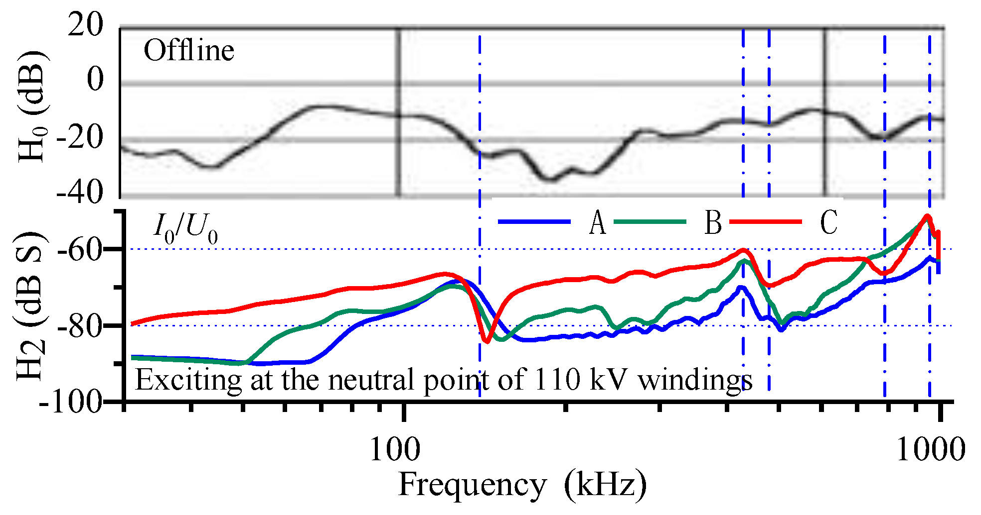
The results of comparison of the transfer functions based on signals from the 110 kV and 10 kV windings are shown in Figure 24 and Figure 25, respectively. The frequencies of some resonances between the curves of the transfer functions were consistent with one another. Some local maxima on the curve of H1 of the 110 kV windings corresponded precisely to the local minima on the curve of H3. Few corresponding resonances were observed between functions H0 and H2 of the 10 kV windings because the excitation signal was at the neutral point of the 110 kV windings when H2 was measured. However, the local extrema on the curve of H2 near 120 kHz and 450 kHz were clearer than those on the curve of H0.
The relationships between the frequency and quality factors of the points of resonance of the transfer functions were complex, and require further research. Our experiment nonetheless proved that the resonant frequency of each function exhibited a certain consistency. Therefore, each transfer function can be used to identify deformations in the windings by the changes of the points of the resonance frequency.
7.3. Factors Influencing Online FRA
In addition to geometrical winding deformations, there are many other factors that affect the inductance and capacitance of a winding, including the magnetic field in the iron core (especially at low frequencies) [20], the temperature and the moisture of the oil–paper insulation system [21,22,23] , and the outside network [24] (which only affects H1–H4).
In offline FRA measurements, the transformer is in almost the same condition during each measurement; therefore, the results of each measurement are usually directly comparable. However, in online FRA measurement, the transformers can be in different conditions during different measurements. The baseline of the amplitude—frequency curves of the network function should thus be selected carefully to maintain the same condition as when the deformation diagnosis was performed.
8. Conclusions
To apply online FRA, new network functions must be established that are not only suited to the configuration of online measurement but are also uninfluenced by the external equipment directly connected to the transformer.Based on multi-port circuit network analysis with comprehensive consideration of the transformers and external electric power grid, three types of network functions, represented by H1–H6, are proposed here. The corresponding suitable conditions and configuration of application are presented.
Functions H1–H4 include the winding neutral-point voltage and current, winding-terminal current, or excitation voltage. They involve the impedances of the outside network, and the outside network must maintain the same configuration.Functions H5 and H6 include the winding neutral-point current and the winding-terminal current. They are unaffected by the outside network, but they require a grounded neutral point.Function.
Simulations based on an three phase transformer model ( refering to a real SFSZ11-220kV/121kV/38.5kV transformer ) were carried out to confirm the feasibility of the above network functions. Sensitivity analyses based on circuit network analysis were carried out. Functions H1 and H2 have less sensitivity than function H0 for offline FRA, and H5 has the same sensitivity as function H0. The results of experiments on a SSZ11-50000/110 transformer showed that the proposed functions contain the same information on electromagnetic resonance as the normal function used in offline FRA. This information can be used to identify defective windings in the transformer while it is operating.
Author Contributions
Conceptualization, S.Y., Y.W. and Y.C.; Methodology, S.Y.; Software, J.L.; Validation, S.Y. and L.C.; Formal analysis, L.C.; Investigation, S.Y.; Resources, Y.W.; Data curation, J.L.; Writing – original draft, S.Y.; Writing – review & editing, Y.C.; Visualization, L.C.; Supervision, S.Y.; Project administration, S.Y.; Funding acquisition, S.Y. All authors have read and agreed to the published version of the manuscript.
Funding
Please add: This research was supported by the project of the State Grid Corporation of Southern China (No. (030100KK52222017/GDKJXM20222322)).
Data Availability Statement
The original contributions presented in this study are included in the article. Further inquiries can be directed to the corresponding author.
Conflicts of Interest
Author S.Y., Y.W., and L.C. were employed by the Electric Power Research Institute of Guangzhou Power Supply Bureau, Guangdong Power Grid. The remaining authors declare that the research was conducted in the absence of any commercial or financial relationships that could be construed as a potential conflict of interest. The authors declare that this study received funding from State Grid Corporation of Southern China. The funder was not involved in the study design, collection, analysis, interpretation of data, the writing of this article or the decision to submit it for publication.
Abbreviations
The following abbreviations are used in this manuscript:
| FRA | Frequency-response analysis |
References
- Amalanathan, J.; Sarathi, R.; Prakash, S.; Mishra, A. K.; Gautam, R.; Vinu, R. Investigation on thermally aged natural ester oil for real-time monitoring and analysis of transformer insulation. High Volt. 2020, vol. 5(no. 2), 209–217. [Google Scholar] [CrossRef]
- Li, Z; He, Y; Xing, Z; et al. Minor fault diagnosis of transformer winding using polar plot based on frequency response analysis[J]. International Journal of Electrical Power & Energy Systems 2023, 152, 109173. [Google Scholar]
- Tan, X; Ao, G; Xu, X; et al. Research on new method of transformer winding deformation detection[J]. Ferroelectrics 2024, 618(9-10), 1851–1866. [Google Scholar] [CrossRef]
- Barros, R. M. R.; da Costa, E. G.; Araujo, J. F.; de Andrade, F. L. M.; Ferreira, T. V. Contribution of inrush current to mechanical failure of power transformers windings. High Volt. 2019, vol. 4(no. 4), 300–307. [Google Scholar] [CrossRef]
- Chen, Y; Zhao, Z; Liu, J; et al. Application of generative AI-based data augmentation technique in transformer winding deformation fault diagnosis[J]. Engineering Failure Analysis 2024, 159, 108115. [Google Scholar] [CrossRef]
- Wu, S; Ji, S; Zhang, Y; et al. A novel vibration frequency response analysis method for mechanical condition detection of converter transformer windings[J]. IEEE Transactions on Industrial Electronics 2023, 71(7), 8176–8180. [Google Scholar] [CrossRef]
- Frequency Response Analysis on Winding Deformation of Power Transformers, People’s Republic of China, Electric Power Industry Standard, DL/T911-2016, ICS27.100, F24, Document No. 53992-2016 (in Chinese), 2016.
- Measurement of Frequency Response, IEC Standard 60076-18, Ed. 1.0, 2012-07, 2012.
- IEEE Guide for the Application and Interpretation of Frequency Response Analysis for Oil-Immersed Transformers, IEEE Std C57.149-2012, pp.1-72, 8 March 2013.
- Behjat, V.; Vahedi, A.; Setayeshmehr, A.; Borsi, H.; Gockenbach, E. Diagnosing shorted turns on the windings of power transformers based upon online FRA using capacitive and inductive couplings. IEEE Trans. Power Del 2011, vol. 26(no. 4), 2123–2133. [Google Scholar] [CrossRef]
- Yao; Zhao, Z.; Chen, Y.; Zhao, X.; Li, Z.; Wang, Y.; Zhou, Z.; Wei, G. Transformer winding deformation diagnostic system using online high frequency signal injection by capacitive coupling. IEEE Trans. Dielectr. Electr. Insul. 2014, vol. 21(no. 4), 1486–1492. [Google Scholar] [CrossRef]
- Rybel, T. D.; Singh, A.; Vandermaar, J. A.; Wang, M.; Marti, J. R.; Srivastava, K. D. Apparatus for online power transformer winding monitoring using bushing tap injection. IEEE Trans. Power Del 2009, vol. 24(no. 3), 996–1003. [Google Scholar] [CrossRef]
- Cheng, Y.; Chang, W.; Bi, J.; Pan, X. Signal injection by magnetic coupling for the online FRA of transformer winding deformation diagnosis. Proc. 1st International Conference on Dielectrics, Montpellier, France, Jul. 2016; pp. 905–908. [Google Scholar]
- Cheng, Y.; Bi, J.; Chang, W.; Xu, Y.; Pan, X.; Ma, X.; Chang, S. Proposed methodology for online frequency response analysis based on magnetic coupling to detect winding deformations in transformers. High Volt. 2020, vol. 5(no. 3), 343–349. [Google Scholar] [CrossRef]
- Rathnayaka, S. B.; See, K. Y.; Prajapati, M.; Li, K.; Narampanawe, N. B.; Fan, F. Inductive coupling method for online frequency response analysis (FRA) for transformer winding diagnostic. 2017 IEEE Region 10 Conference, Penang, 2017; pp. 88–92. [Google Scholar]
- Zhang, Z. RETRACTED: Characterizing transformer HV–LV winding FRA curves through derivation of transfer functions from FRA data[J]. 2024.
- Tarimoradi, H; Karami, H; Gharehpetian, G B; et al. Sensitivity analysis of different components of transfer function for detection and classification of type, location and extent of transformer faults[J]. Measurement 2022, 187, 110292. [Google Scholar] [CrossRef]
- Beheshti Asl, M; Fofana, I; Meghnefi, F; et al. A comprehensive review of transformer winding diagnostics: Integrating frequency response analysis with machine learning approaches[J]. Energies 2025, 18(5), 1209. [Google Scholar] [CrossRef]
- Hosseini, A; Abbasi, A; Abbasi, A R; et al. Transformer windings defects identification using frequency response analysis and advanced data visualization techniques[J]. Scientific Reports 2025, 15(1), 40595. [Google Scholar] [CrossRef] [PubMed]
- Thango, B A; Nnachi, A F; Dlamini, G A; et al. A novel approach to assess power transformer winding conditions using regression analysis and frequency response measurements[J]. Energies 2022, 15(7), 2335. [Google Scholar] [CrossRef]
- Larin, V. Internal short-circuits faults localization in transformer windings using FRA and natural frequencies deviation patterns. CIGRE SC A2 Colloquium, Cracow, Poland, 2017. [Google Scholar]
- Bagheri, M; Phung, B T; Blackburn, T. Influence of temperature and moisture content on frequency response analysis of transformer winding[J]. IEEE Transactions on Dielectrics and Electrical Insulation 2014, 21(3), 1393–1404. [Google Scholar] [CrossRef]
- Beheshti Asl, M; Fofana, I; Meghnefi, F; et al. A comprehensive review of transformer winding diagnostics: Integrating frequency response analysis with machine learning approaches[J]. Energies 2025, 18(5), 1209. [Google Scholar] [CrossRef]
- Shanmugam, N; Gopal, S; Madanmohan, B; et al. Diagnosis of inter-turn shorts of loaded transformer under various load currents and power factors; impulse voltage-based frequency response approach[J]. Ieee Access 2021, 9, 40811–40822. [Google Scholar] [CrossRef]
Figure 1.
Equivalent two-port network of a transformer winding.
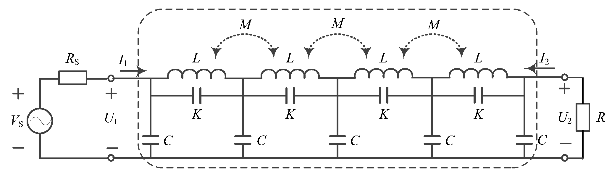
Figure 2.
Principle of excitation-signal injection: (a) schematic diagram; (b)equivalent circuit.
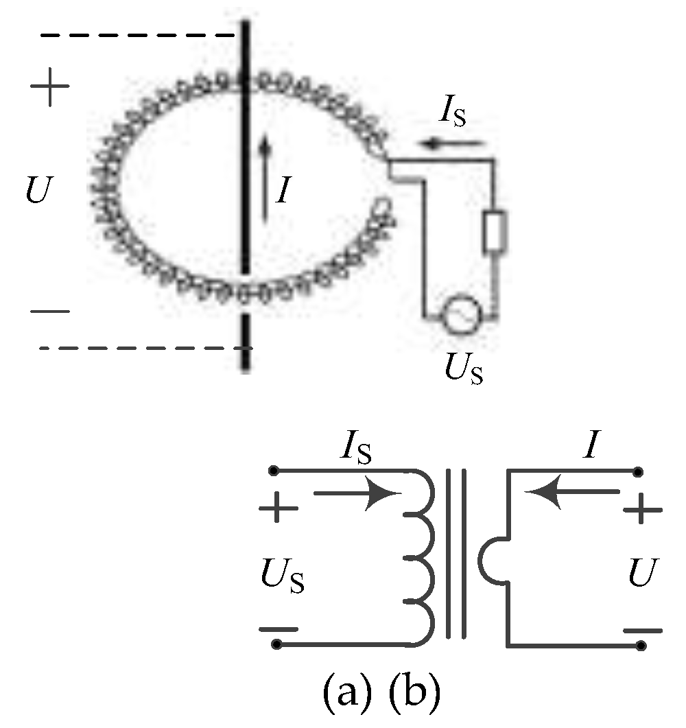
Figure 3.
Rogowski coil current sensor at the root of the HV bushing.
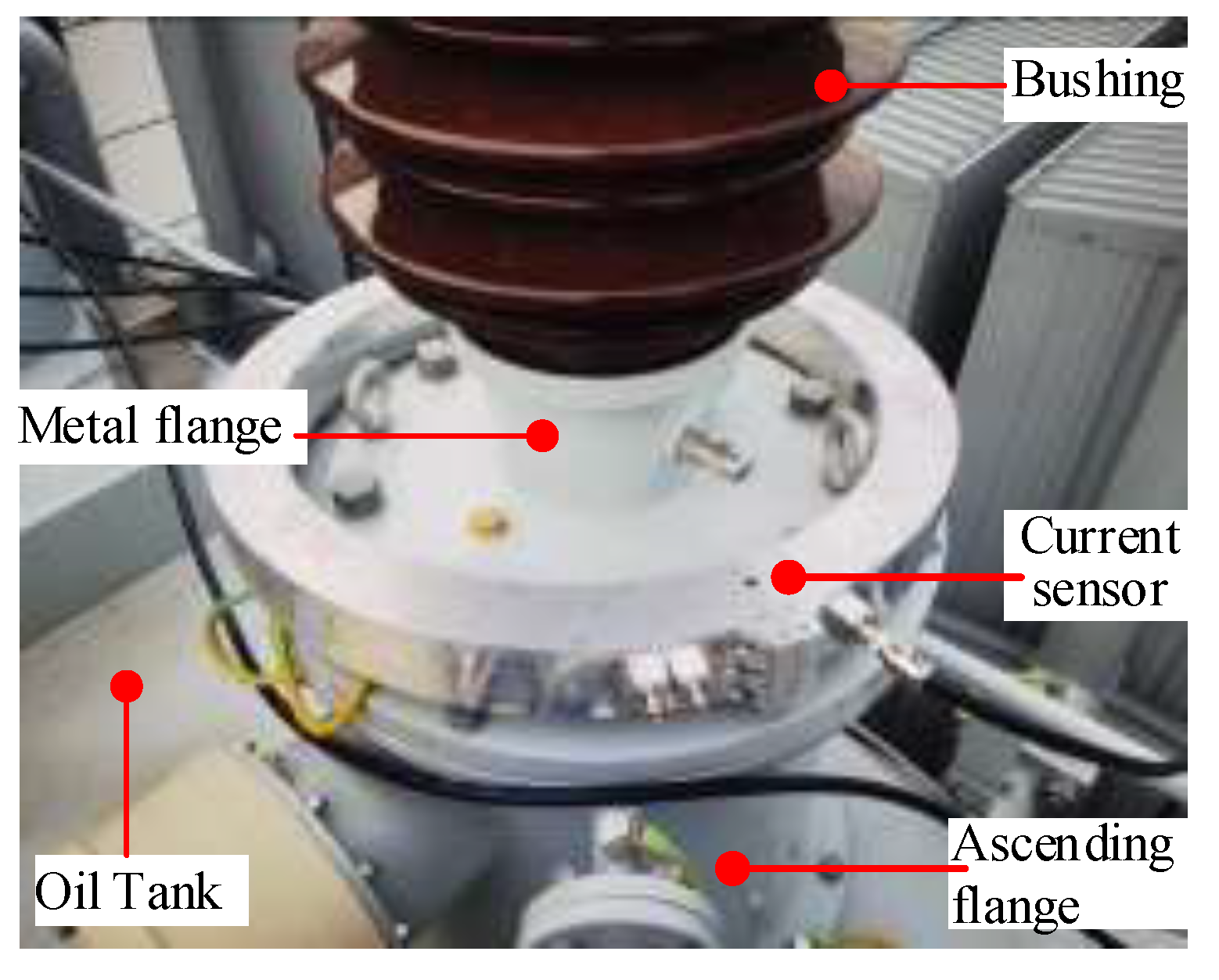
Figure 4.
Schematic diagram of online FRA application: (a) schematic diagram; (b) experimental scenario.
Figure 4.
Schematic diagram of online FRA application: (a) schematic diagram; (b) experimental scenario.
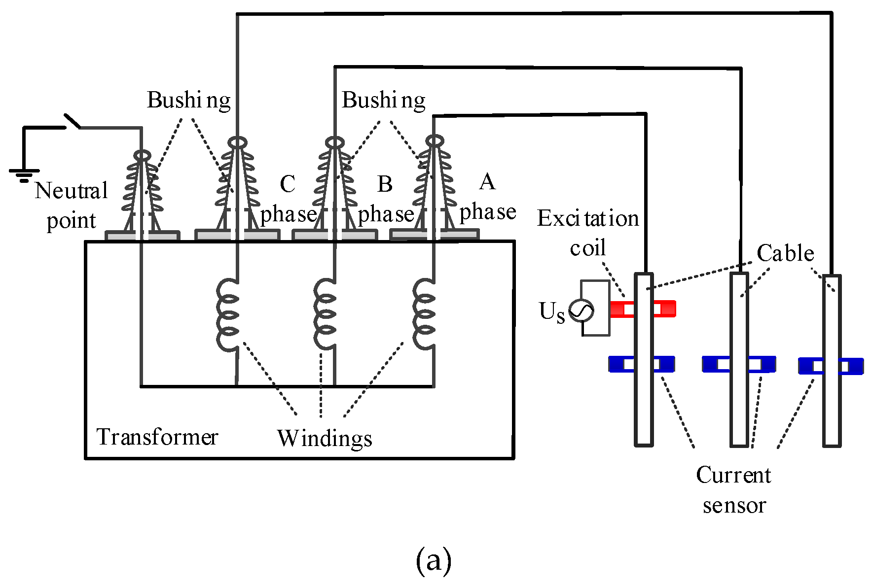
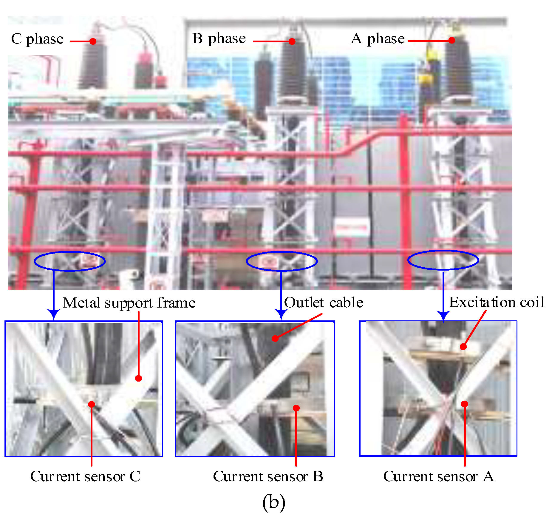
Figure 5.
Part of the network outside of the transformer.
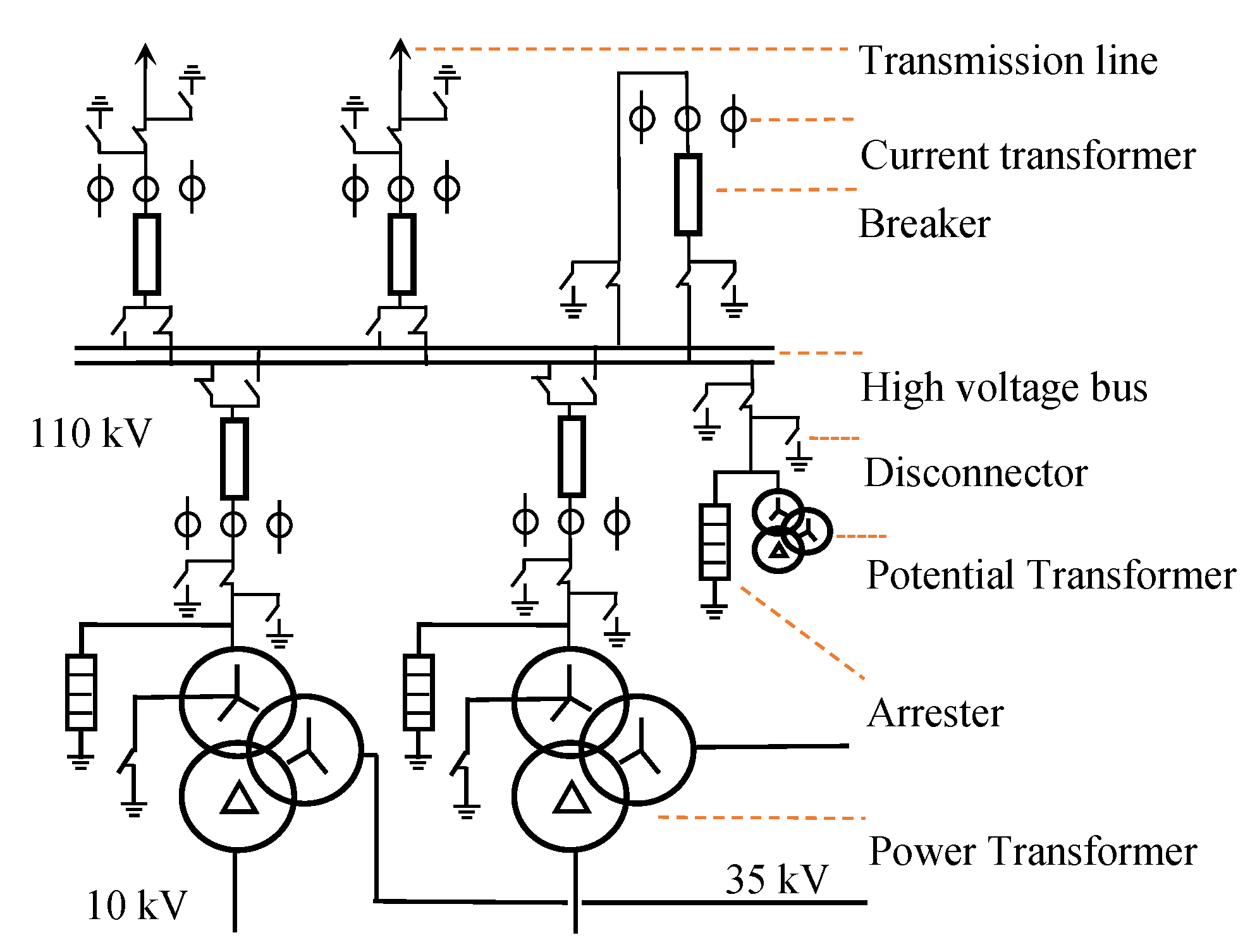
Figure 6.
Schematic diagram of windings with grounded neutral point.
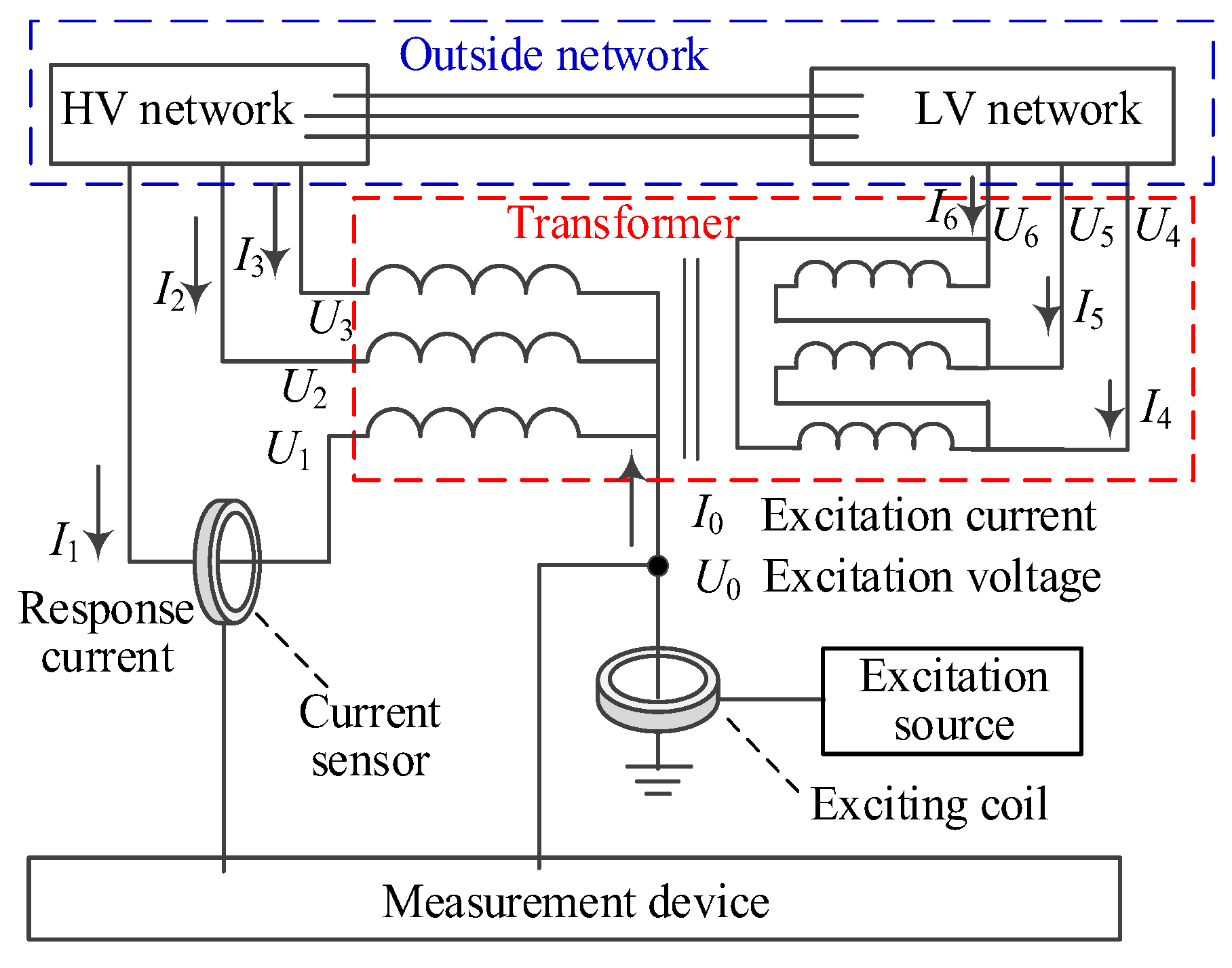
Figure 7.
Schematic diagram of windings without grounded neutral point.
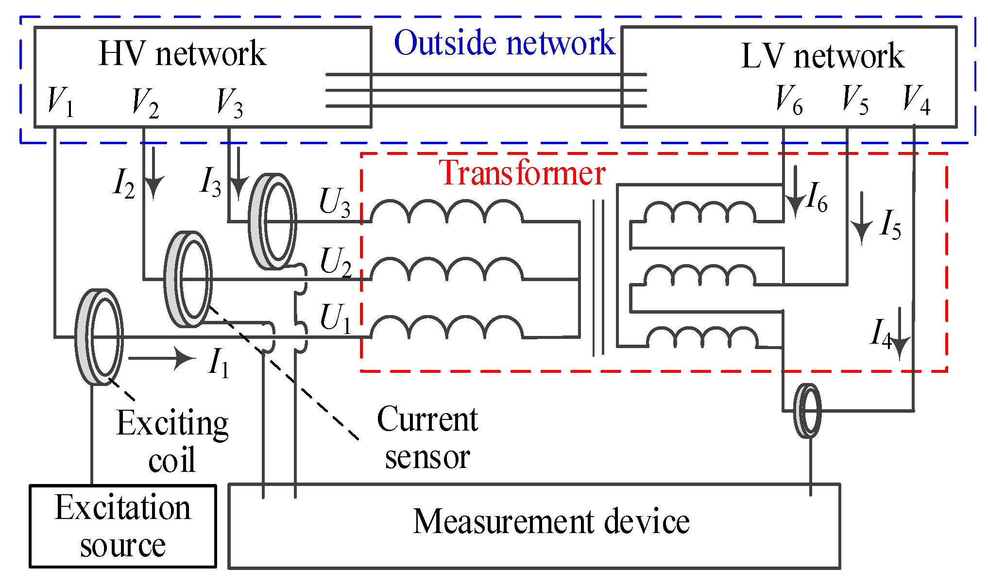
Figure 8.
Schematic diagram of windings with grounded neutral point and injection at the HV terminal of the winding.
Figure 8.
Schematic diagram of windings with grounded neutral point and injection at the HV terminal of the winding.
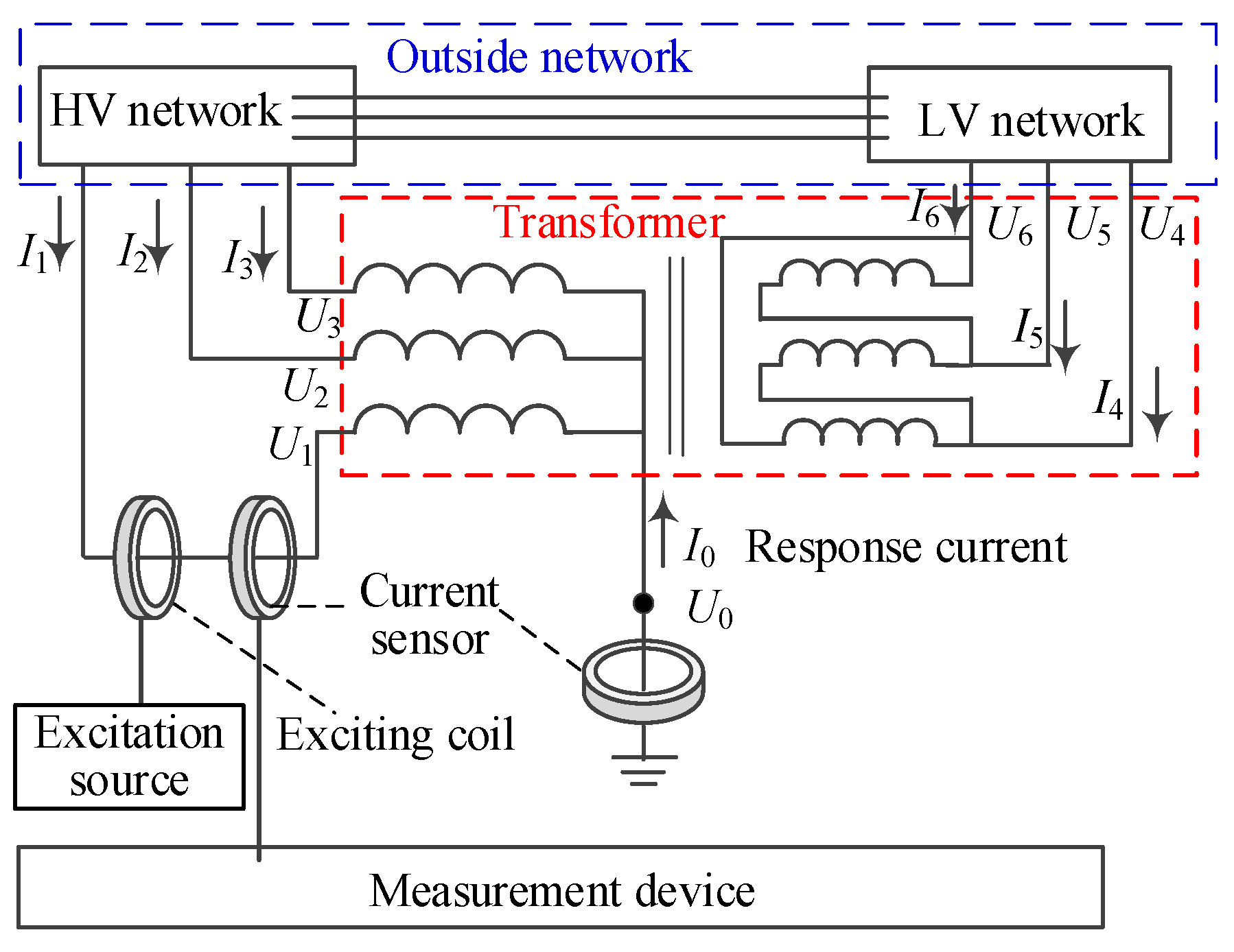
Figure 9.
Finite-element model of one-phase windings.
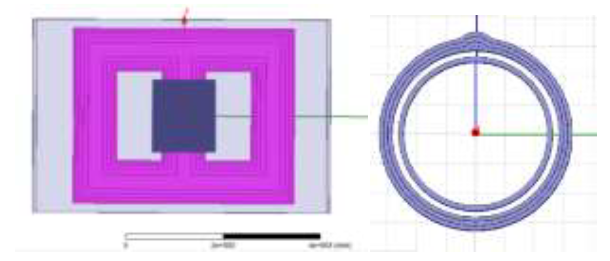
Figure 10.
Amplitude–frequency curve of H2 ( j=1. It was about the A phase HV winding. The bulge was on the A phase HV winding ).
Figure 10.
Amplitude–frequency curve of H2 ( j=1. It was about the A phase HV winding. The bulge was on the A phase HV winding ).
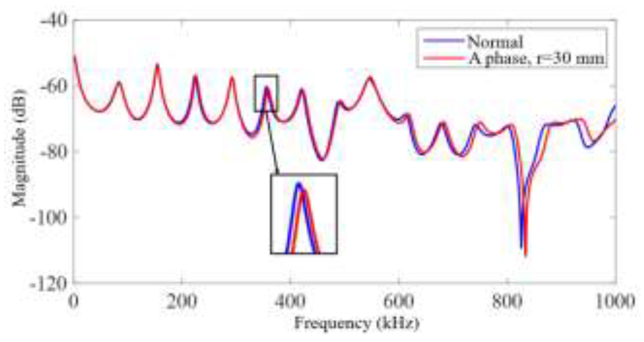
Figure 11.
Amplitude–frequency curve of H3 (The excitation signal was injected at the HV terminal of the A phase. The response currents were meausred at the HV terminals of the B phase and C phase. The bulge was on the B phase HV winding ).
Figure 11.
Amplitude–frequency curve of H3 (The excitation signal was injected at the HV terminal of the A phase. The response currents were meausred at the HV terminals of the B phase and C phase. The bulge was on the B phase HV winding ).
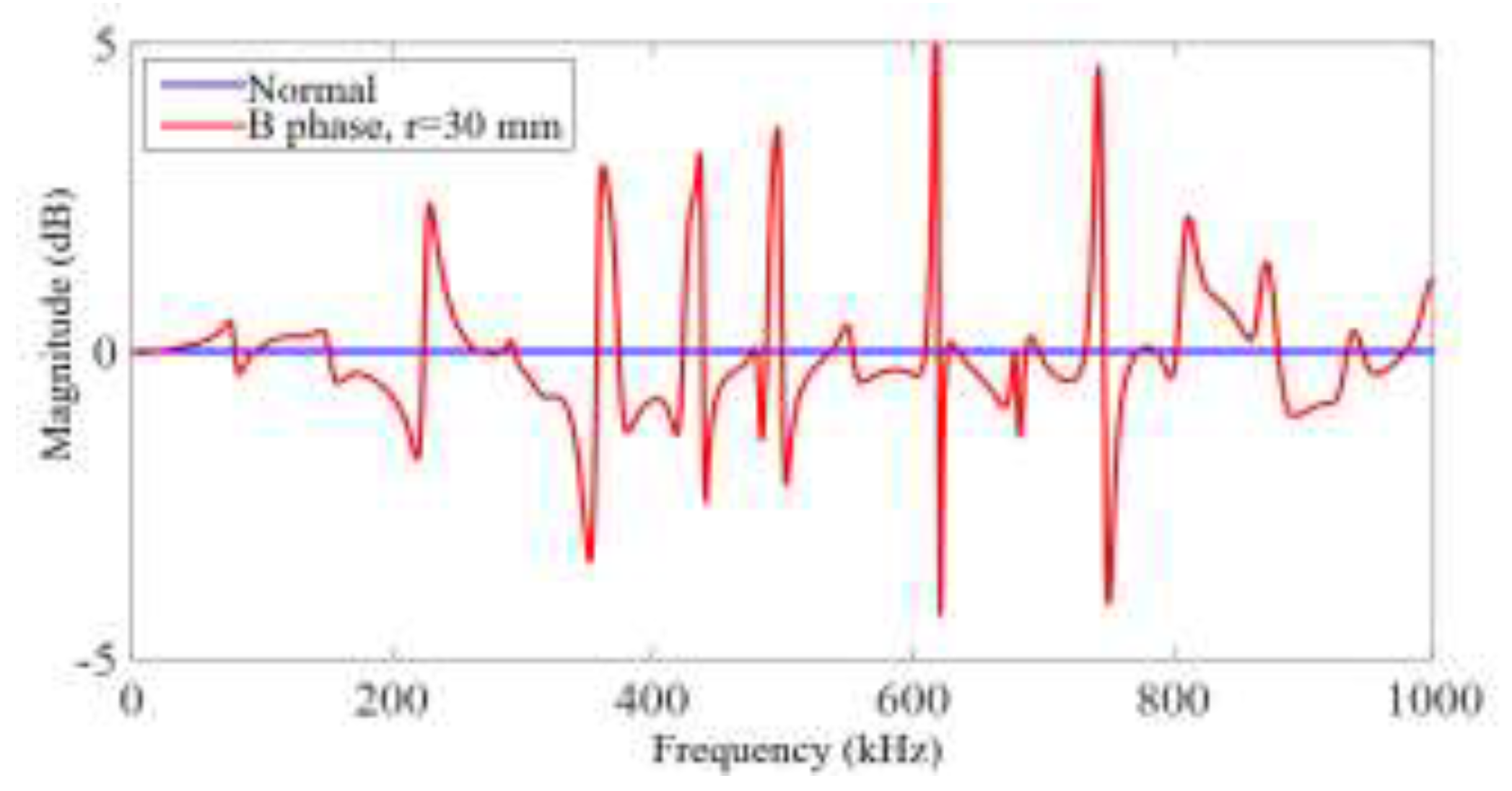
Figure 12.
Amplitude–frequency curve of H5 ( It was about the A phase HV winding. The bulge was on the A phase HV winding ).
Figure 12.
Amplitude–frequency curve of H5 ( It was about the A phase HV winding. The bulge was on the A phase HV winding ).
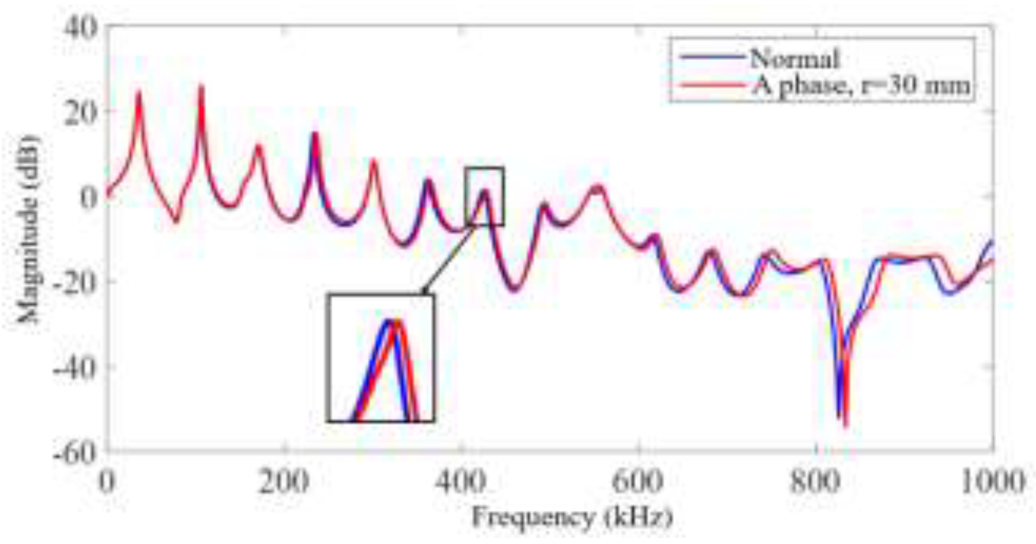
Figure 13.
Current sensor of the Rogowski coil at the root of the HV bushing.
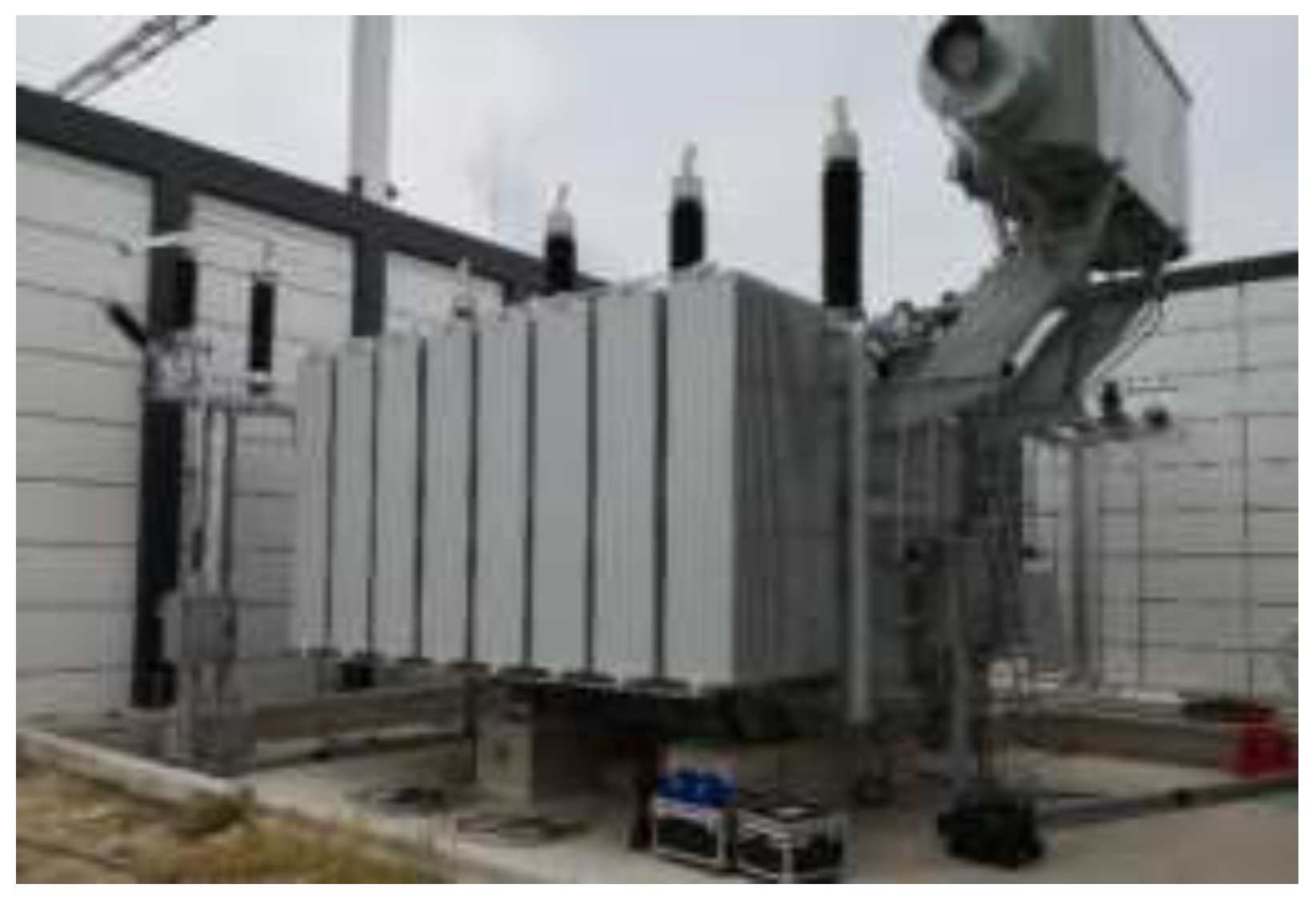
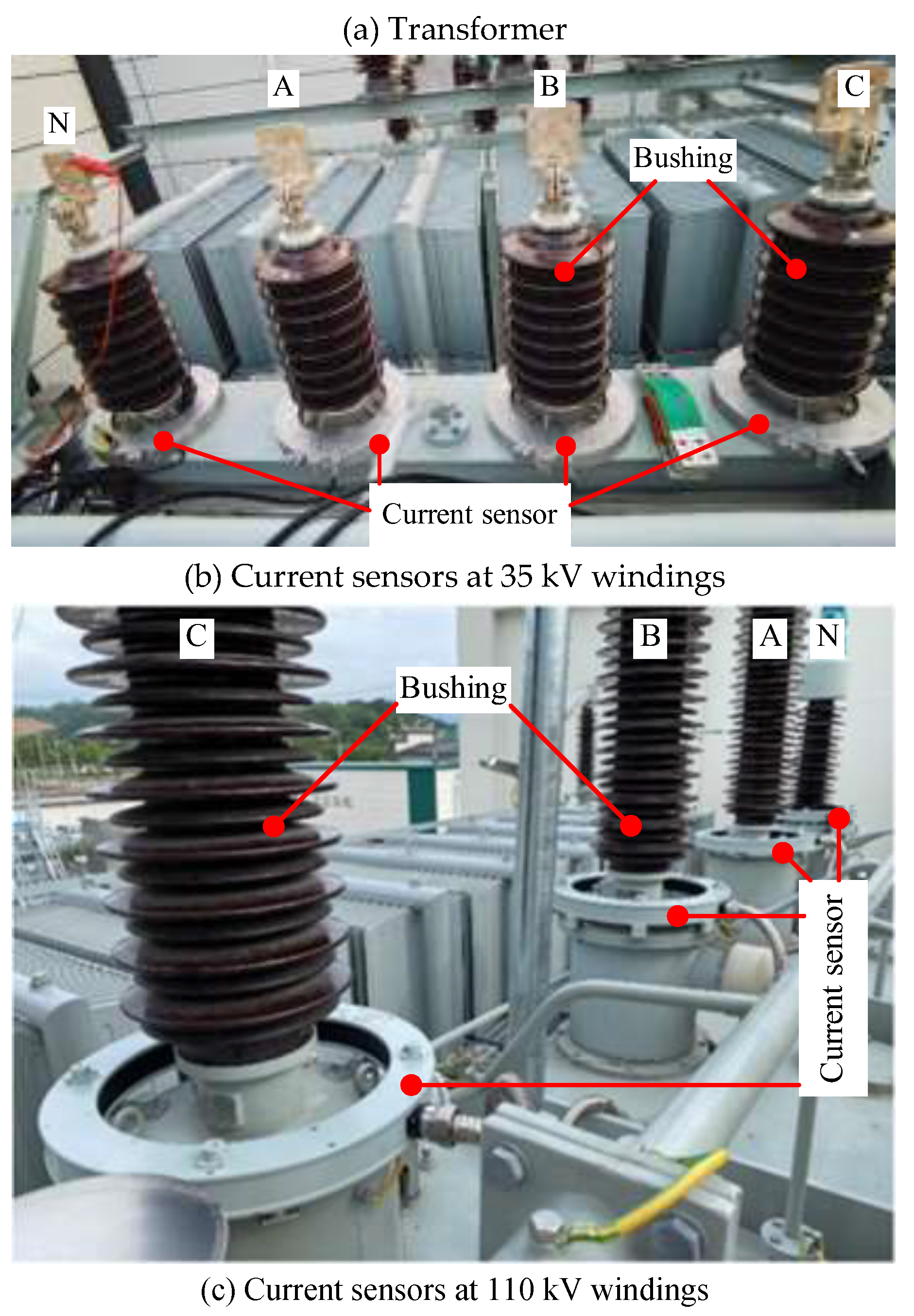
Figure 14.
Curves of the transfer function H0 of the transformer in Figure 7 when measured offline.
Figure 14.
Curves of the transfer function H0 of the transformer in Figure 7 when measured offline.
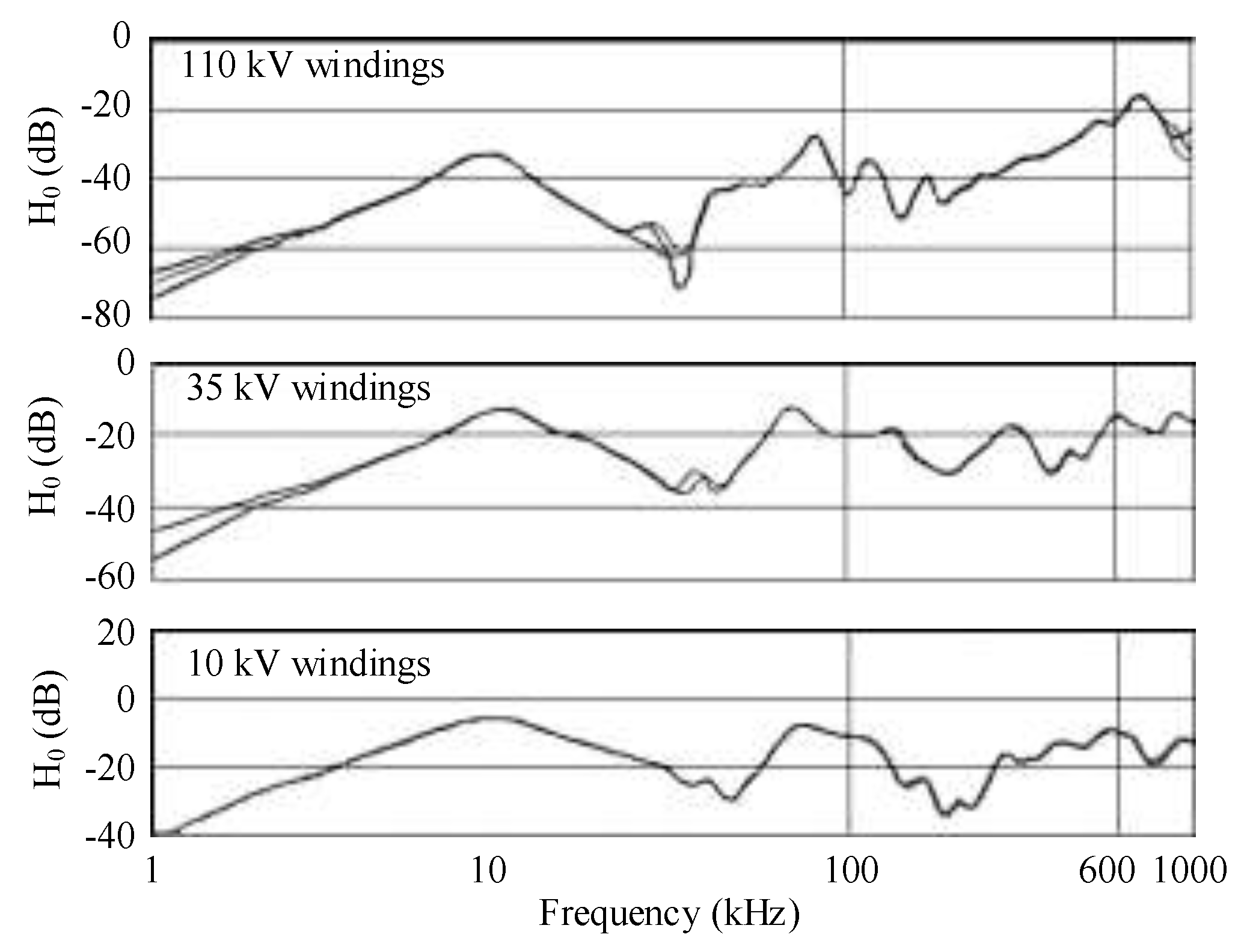
Figure 15.
Scenario of installation of the excitation coil at the bushing of the neutral point of the windings with a voltage of 35 kV.
Figure 15.
Scenario of installation of the excitation coil at the bushing of the neutral point of the windings with a voltage of 35 kV.
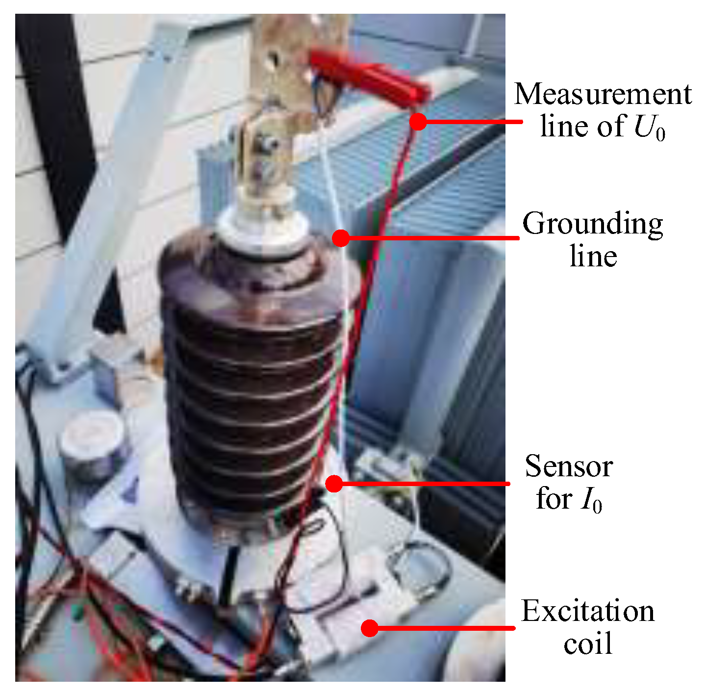
Figure 16.
Signals of the excitation voltage and the response current at 302 kHz on 35 kV windings.
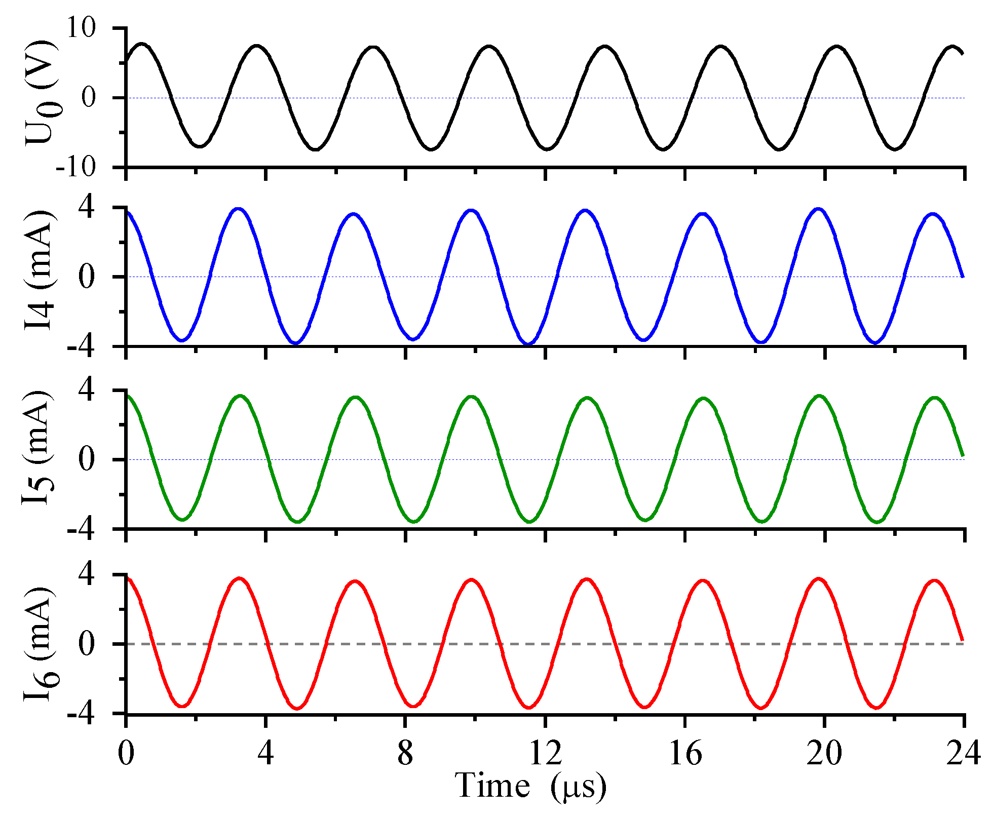
Figure 17.
Amplitude–frequency curves of transfer function H1.
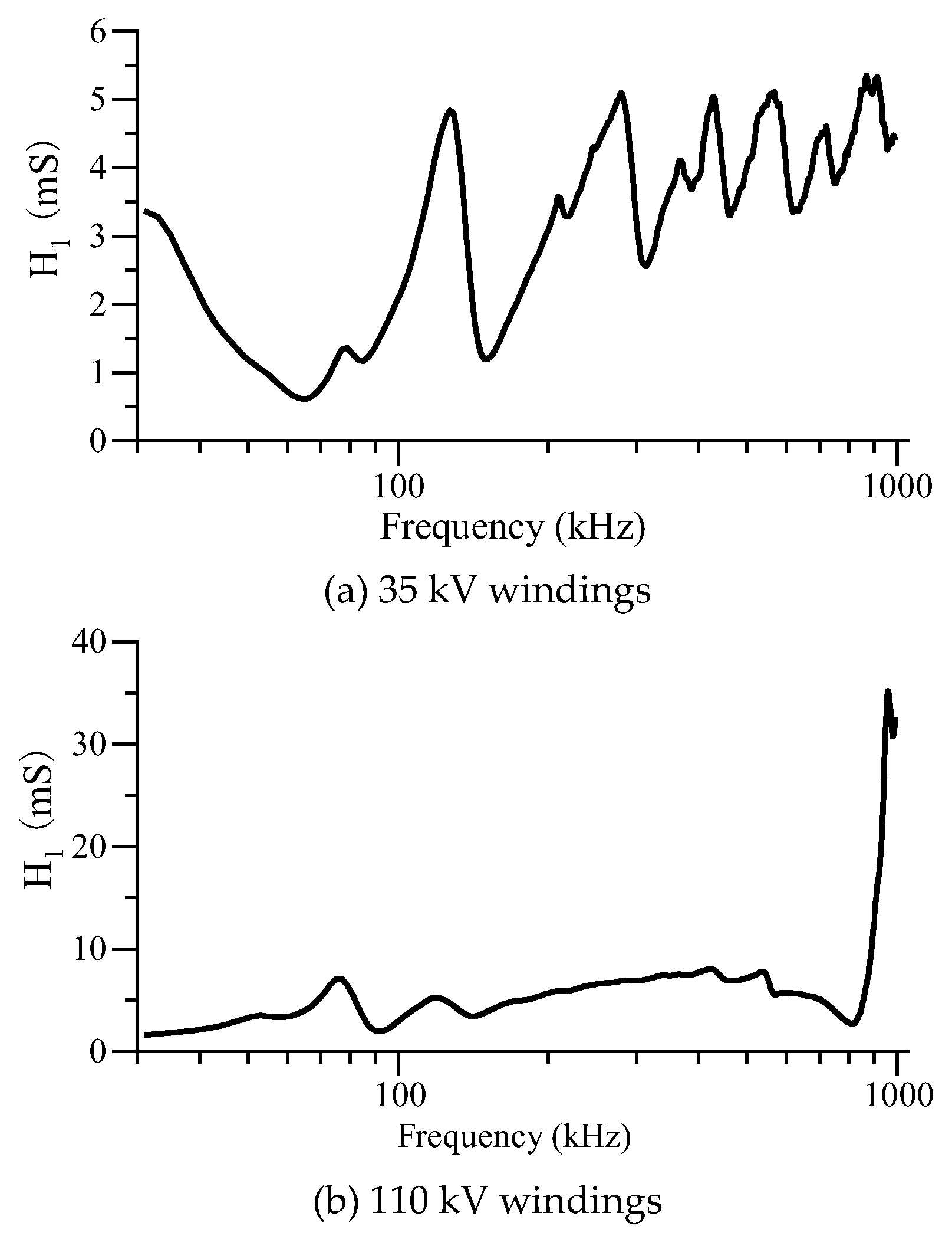
Figure 18.
Amplitude–frequency curves of transfer function H2 of windings with a rated voltage of 35 kV (the excitation coil was located at the neutral point of the winding).
Figure 18.
Amplitude–frequency curves of transfer function H2 of windings with a rated voltage of 35 kV (the excitation coil was located at the neutral point of the winding).
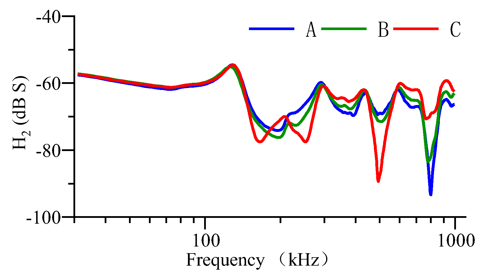
Figure 19.
Amplitude–frequency curves of transfer function H2 of 35 kV windings (the excitation coil was located at the neutral point of the 110 kV windings).
Figure 19.
Amplitude–frequency curves of transfer function H2 of 35 kV windings (the excitation coil was located at the neutral point of the 110 kV windings).
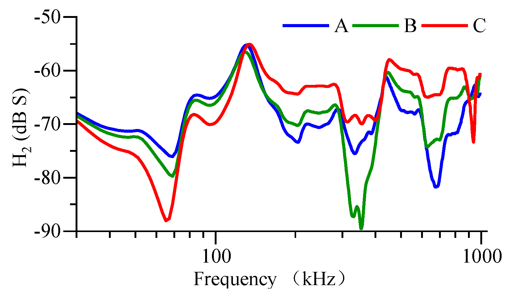
Figure 20.
Amplitude–frequency curves of transfer function H2 of 10 kV windings (the excitation coil was located at the neutral point of the 110 kV windings).
Figure 20.
Amplitude–frequency curves of transfer function H2 of 10 kV windings (the excitation coil was located at the neutral point of the 110 kV windings).
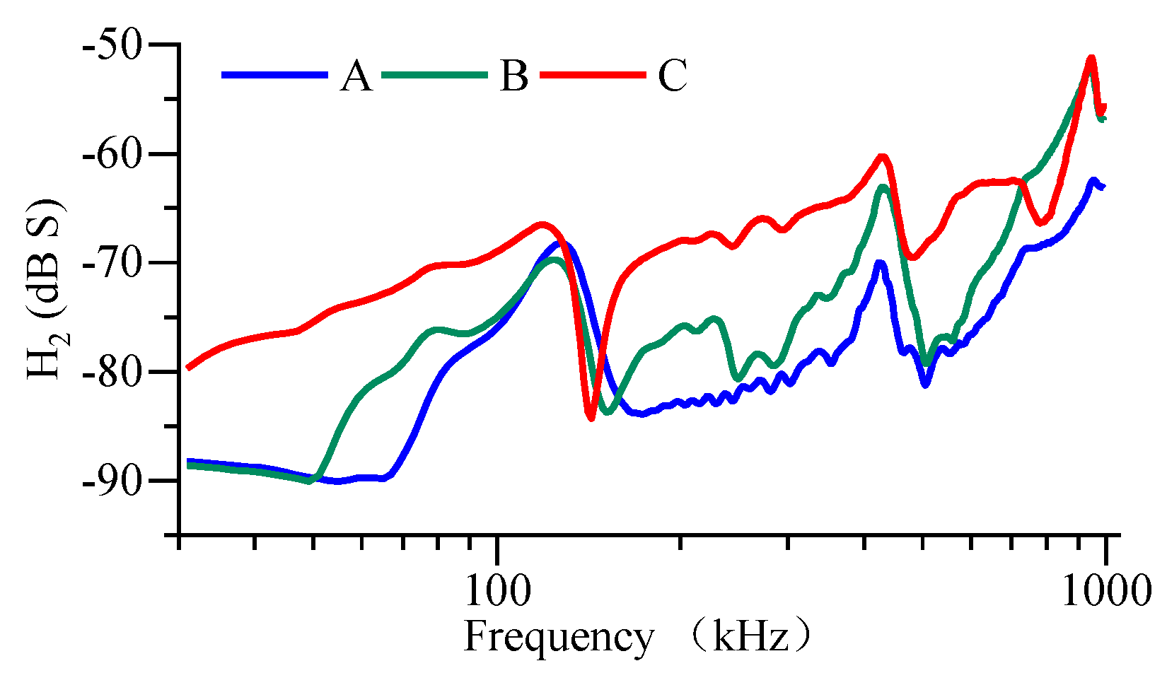
Figure 21.
Amplitude–frequency curves of transfer function H3 of 110 kV windings (the excitation coil was located at the neutral point of the 110 kV windings).
Figure 21.
Amplitude–frequency curves of transfer function H3 of 110 kV windings (the excitation coil was located at the neutral point of the 110 kV windings).
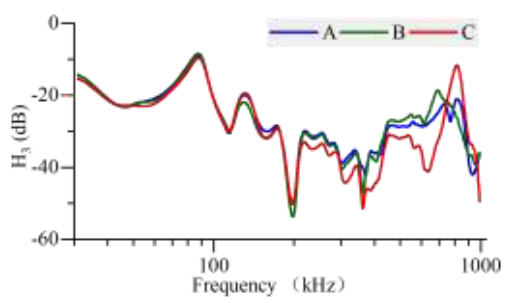
Figure 22.
Amplitude–frequency curve of transfer function H4 of 35 kV windings (the excitation coil was located at the HV terminal of the A-phase windings).
Figure 22.
Amplitude–frequency curve of transfer function H4 of 35 kV windings (the excitation coil was located at the HV terminal of the A-phase windings).
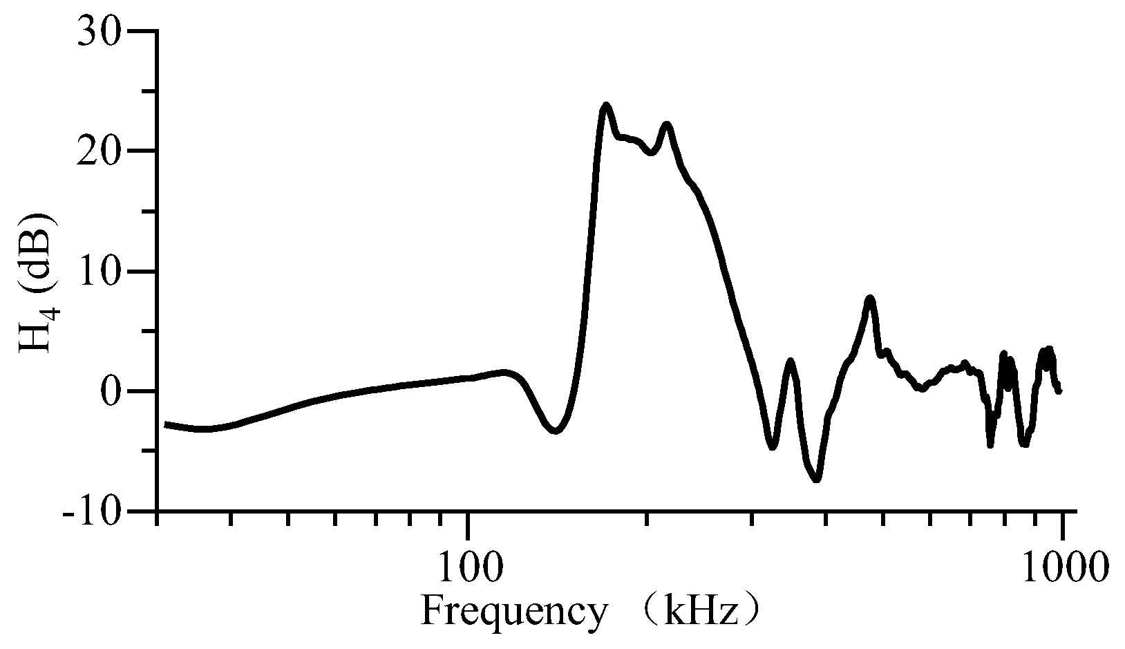
Figure 23.
Corresponding resonance points of the transfer functions based on signals of 35 kV windings.
Figure 23.
Corresponding resonance points of the transfer functions based on signals of 35 kV windings.
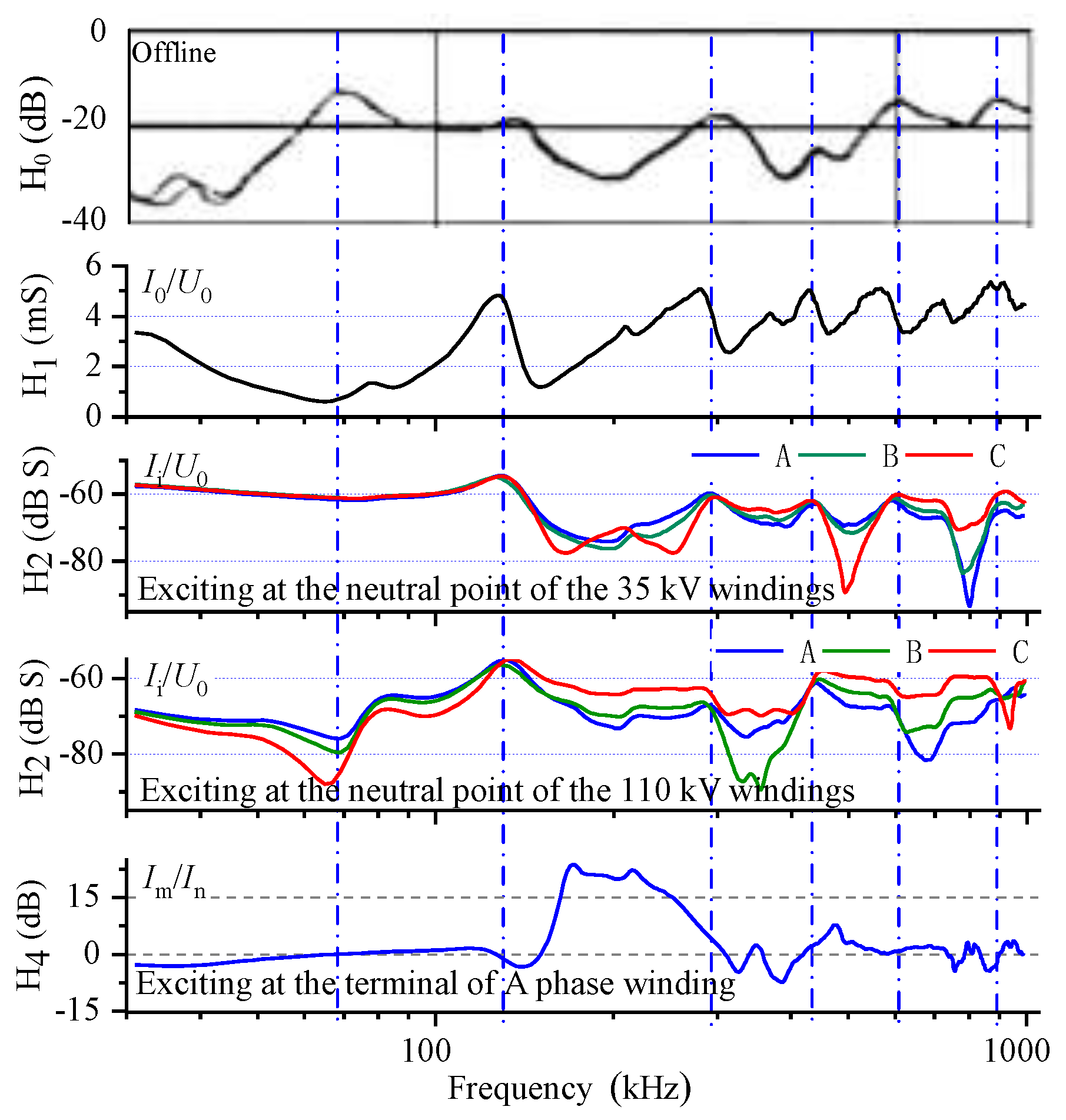
Figure 24.
Corresponding resonance points of the transfer functions based on signals of 110 kV windings.
Figure 24.
Corresponding resonance points of the transfer functions based on signals of 110 kV windings.
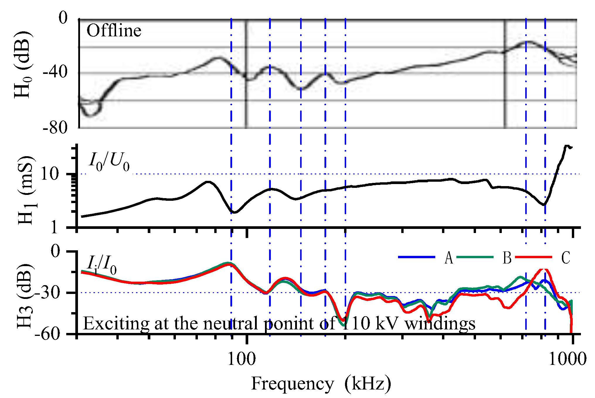
Figure 25.
Corresponding resonance points of the transfer functions based on signals of 10 kV windings.
Figure 25.
Corresponding resonance points of the transfer functions based on signals of 10 kV windings.
Disclaimer/Publisher’s Note: The statements, opinions and data contained in all publications are solely those of the individual author(s) and contributor(s) and not of MDPI and/or the editor(s). MDPI and/or the editor(s) disclaim responsibility for any injury to people or property resulting from any ideas, methods, instructions or products referred to in the content. |
© 2026 by the authors. Licensee MDPI, Basel, Switzerland. This article is an open access article distributed under the terms and conditions of the Creative Commons Attribution (CC BY) license (http://creativecommons.org/licenses/by/4.0/).
Copyright: This open access article is published under a Creative Commons CC BY 4.0 license, which permit the free download, distribution, and reuse, provided that the author and preprint are cited in any reuse.


