
Submitted:
27 January 2026
Posted:
28 January 2026
You are already at the latest version
Abstract
As an information extraction framework, graph neural network has been widely used in many fields, but there is a serious problem of over-smoothing in graph neural network, that is, with the increase of the number of iterations, the nodes gradually tending toward similarity, resulting in reduced feature distinguishability and deteriorated model performance. In order to solve this problem, this paper proposes a novel solution, that is, to alleviate the over-smoothing problem in graph neural networks from the perspective of changing the topological information dimension. This article uses graph regularization to solve this problem, by fine-tuning the topology structure, the research objectives can be achieved, and demonstrated through extensive ablation experiments, a large number of experiments verify the effectiveness and feasibility of the proposed method. Physically speaking, this method limits the connection strength of the adjacency matrix to a finite number of steps; The higher the order, the more obvious the restriction effect, therefore, it can alleviate the problem of over smoothing in graph neural networks to a certain extent.
Keywords:
GCN
; topological symmetry limitation
; graphic regularization
; over-smoothing
1. Introduction
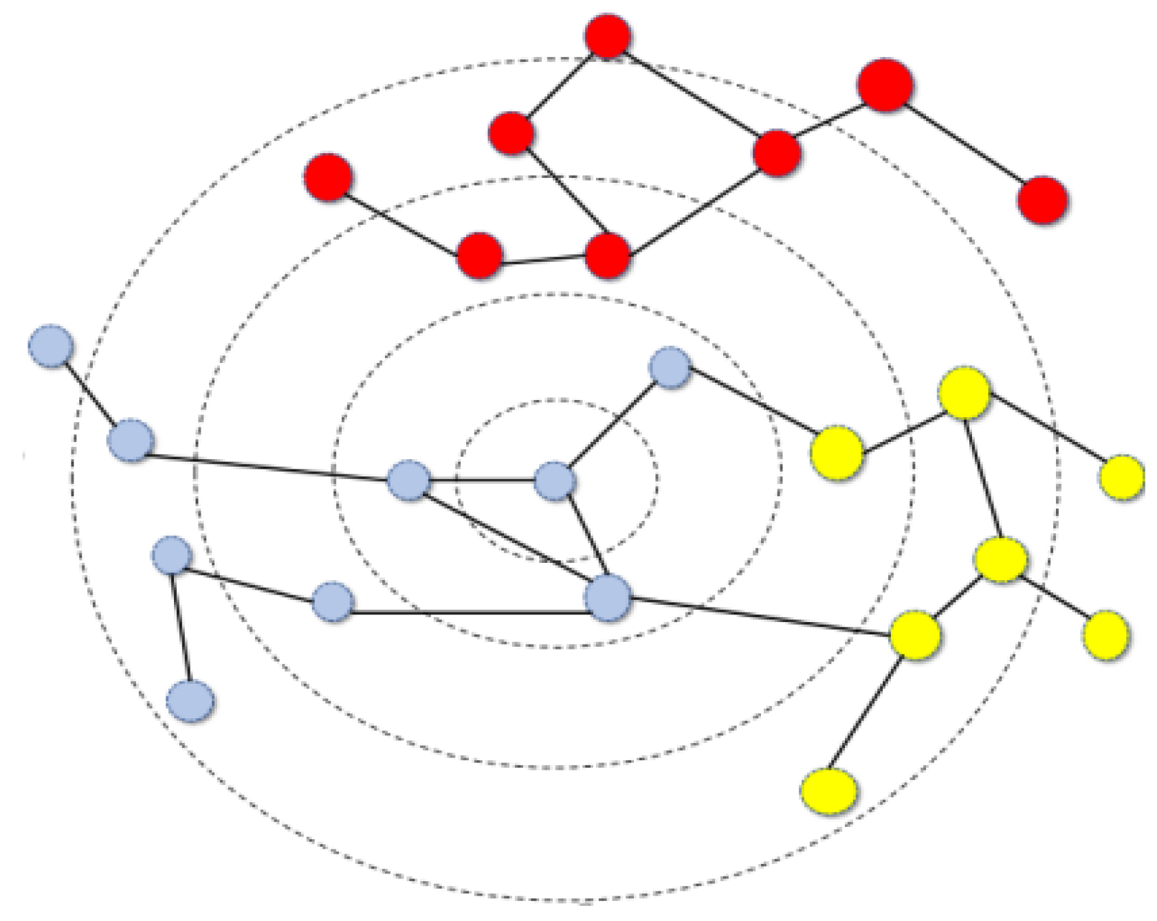
The existing methods for solving the over smoothing [1,2,3,4] problem lack qualitative research on the relationship between the over smoothing problem[5] and the topological structure[6,7] of the graph. From the perspective of topology, why does the over-smoothing problem occur, and how to start with topological information to alleviate this problem is challenging. This begs us to start thinking about the data structure of graph data. The graph data has a certain uniqueness. Compared with structured data and streaming data, there is a strong topological relationship between data points, and there may be certain commonalities and differences between the connected points in the topological structure.As shown in the figure below, for the blue node located in the center of the graph, when the number of GNN layers is 1, the neighbor nodes in the sensing field are all blue nodes of the same kind, and with the increase of the number of GNN layers, two heterogeneous nodes will increase in the sensing field, and the noise will increase. Therefore, the embedding learned in the vector space[8,9] tends to be consistent and produces an over-smoothing problem. However, when the signal-to-noise ratio is high, the problem of graph over smoothing is severe. When the signal-to-noise ratio is low, the problem of graph over smoothing is not severe. Therefore, by reducing the signal-to-noise ratio of the graph, it can alleviate the problem of graph over smoothing. Compared with previous methods of designing new GNN topology structures to alleviate the problem of over smoothing, this approach has the advantages of low cost, low time complexity, and high robustness of the model[10].
Figure 1.
we present an overview of our approach architecture. The loss function is composed of three distinct components: the MLP Layer Loss, the BQBT to AK Loss, and the GCN Loss.
Figure 1.
we present an overview of our approach architecture. The loss function is composed of three distinct components: the MLP Layer Loss, the BQBT to AK Loss, and the GCN Loss.
We solve this problem through graph regularization method. Article creatively proposes a qualitative measurement standard as a regularization term, is embedded into the process of graph representation learning. The principle is to improve the signal-to-noise ratio[11,12] of node features during propagation by limiting the link strength of the adjacency matrix in a finite number of steps, thereby indirectly alleviating the problem of over smoothing in graph neural networks. This approach can alleviates the problem of over-smoothing, and it suggests that one of the causes of oversmoothing is the excessive mixing of information and noise[13,14]. To prove our hypothesis that improving the topology of a graph is helpful in exploring the smoothness of its representation, we propose adding the regularization term of BQBT− > Ak , through experimental results show that our method can significantly alleviate the problem of over-smoothing in graph neural networks,and it can improve the performance of the model to a certain extent[15,16], it provide a striking perspective for better improving the performance of GNN. The contribution of this work is twofold: asystematic and qualitative study of the problem of over-smoothing, which verifies that a key factor behind the over-smoothing problem is the impact of changes in node signal-to-noise ratio on topology.
2. Materials and Methods
Next, we will present the work of this article in a step-by-step manner, moving from the overall structure to more detailed, partial aspects.
2.1. Problem Definition
This paper seeks to undertake a thorough and qualitative exploration into the prevalent issue of oversmoothing within a varied array of graph datasets and models.
Definition 1: A graph can be formulated as G = (V, E), where V is the set of nodes and E is the set of edges. In a more detailed sense, a graph is a structure that depicts relationships between objects[17,18,19], with the nodes representing the objects and the edges signifying the connections or interactions between them.
Figure 2.
we present an overview of our approach architecture. The loss function is composed of three distinct components: the MLP Layer Loss, the BQBT to AK Loss, and the GCN Loss.
Figure 2.
we present an overview of our approach architecture. The loss function is composed of three distinct components: the MLP Layer Loss, the BQBT to AK Loss, and the GCN Loss.
In an attributed graph, the node attributes can be defined as a matrix X in which each row corresponds to a specific node in the graph. These attributes provide additional information about the nodes[20,21,22], enhancing our understanding and analysis of the graph’s structure and behavior. The attributes can encompass a diverse range of characteristics such as numerical values[23,24], categorical labels[25,26], or even textual descriptions. Each attribute contributes to the overall representation of the node, enabling more sophisticated graph algorithms and applications. For instance, in a social network graph, node attributes might include personal information like age, gender, occupation, or interests, which can be crucial for analyzing social patterns and interactions.
Furthermore, the matrix X can be utilized in various graph processing techniques, including machine learning algorithms for node classification[27,28], link prediction[29,30], or community detection[32]. By leveraging the node attributes, these algorithms can achieve more accurate and insightful results. For example, in recommendation systems[33,34], the attributes of user nodes can be used to make personalized recommendations based on the users’ preferences and behavior. In the field of bioinformatics[35,36], node attributes in gene regulatory networks can help in identifying key genes and understanding the complex interactions within biological systems.
In summary, the concept of node attributes in attributed graphs extends the basic graph structure by incorporating valuable information about the nodes, facilitating advanced graph analytics and enabling a wide range of practical applications across diverse domains.
Definition 2: Given the labels Y ∈ R n∗c for all nodes and the adjacency matrix A ∈ {0, 1} n×n, The block matrix is defined as:
H = YTAY ⊘ YTAE
In this formulation, E denotes an all-ones matrix that is of the same dimensions as Y, and ⊘ represents the Hadamard element-wise division operation. The block matrix serves to model the probability distribution of different blocks being connected by an edge. In the present work, the blocks symbolize the various classes of labels within a graph. From a node-wise perspective, Hi,i signifies the likelihood that a node bearing the i-th class forms a connection with a node of the j-th class.
Definition 3: We propose a quantitative metric, BQBT → AK, Q = (HH) T, to evaluate the over-smoothness of graph node representations. This regularization, BQBT → AK, is added to optimize graph topology. K refers to the number of layers, by designing this operator (BQBT), the adjacency matrix can be implicitly representedApply regularization to prevent infinite amplification of connection strength in multi-layer propagation (i.e., solve the problem of over smoothing). In a sense, it is equivalent to breaking the phenomenon of infinite amplification[37,38] of connection strength in the process of multi-layer propagation, and breaking the symmetry in the propagation process.
2.2. The Significance of This Metric Lies in Its Unique Formation Process
As detailed in Equation (1). Since the computation of the block matrix necessitates complete labels, we rely solely on node attributes to generate soft labels. To achieve this, we utilize a multilayer perceptron (MLP), which transforms node attributes into soft labels as shown in Equation (2): B = σ(MLP(X)), where X represents the node attributes, B is the output of the MLP, and σ(·) denotes the activation function. This process is crucial in the pre-training stage, where the loss function for the multi-layer perceptron is optimized to enhance the quality of node representations.
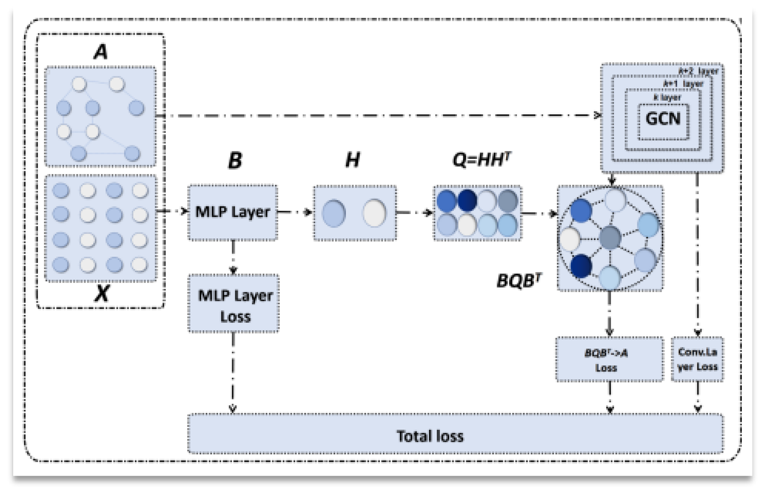
In Figure 3. we present an overview of our approach architecture. The loss function is composed of three distinct components: the MLP Layer Loss, the BQBT to AK Loss, and the GCN Loss.
MLP = X vi∈Tv (Bi , Yi)
In this formulation, Bi denotes the soft label assigned to a given node, while Yi indicates the ground-truth label corresponding to node vi. The collection of nodes taken into account, denoted as τν, constitutes the training set. The function f(·) represents the cross entropy. The comprehensive loss for our model encompasses the combination of the GCN (Graph Convolutional Network) loss and the MLP (Multi-Layer Perceptron) loss, as utilized in our approach.
i.e finalloss = gcnloss + mlploss + ⋋ ∗ loss2
loss2 = F.mseloss(torch.mm(torch.mm(B, Q), B.t()), adjk )
2.3. Model Optimization
Similar to the MLP layer (Eq.3),our method adopts a semi-supervised loss as L, GCN = X vi∈Tv (Zi , Yi) (6)
Specifically, our innovative method intricately integrates the MLP (Multi-Layer Perceptron) layer with the subsequent modules, seamlessly weaving them into an overall robust framework. This integration not only preserves the essential loss function of the MLP layer but also enhances it by incorporating additional components. As a result, the final loss function emerges as a harmonious blend, encapsulating the strengths of each element and facilitating more efficient training and superior performance in various machine learning tasks.
finalloss = gcnloss + mlploss + ⋋ ∗ BQBT− > Ak
where λ is the balance parameter (with the default value 0.5).
3. Results
Datasets
We conduct experiments on three real-world datasets[39,40], namely Cora, Citeseer, and Pubmed [41,42]. These datasets are widely used in the field of graph-based machine learning and have been employed in numerous studies to evaluate the performance of various algorithms. The Cora dataset, for instance, consists of scientific publications classified into one of seven research areas. The Citeseer dataset is similar in nature, comprising academic papers that are categorized into six distinct topics. On the other hand, the Pubmed dataset is more focused on the medical domain, featuring research articles related to diabetes.The number of nodes, features, edges, classes, the partitioning method of the training, validation, and test sets, as well as the task type of these datasets are summarized in Table 1. Each of these datasets presents unique challenges and characteristics, making them ideal for assessing the effectiveness of our proposed approach. For example, the Cora dataset has a relatively high number of features compared to the number of nodes, which can pose difficulties in feature selection and dimensionality reduction techniques. In contrast, the Citeseer dataset has a more balanced ratio of features to nodes but contains a larger number of edges, indicating a more intricate graph structure.Furthermore, the partitioning of the datasets into training, validation, and test sets plays a crucial role in the evaluation process. The partitioning method ensures that the model is trained on a representative subset of the data and tested on an independent set to avoid overfitting. Table 1 provides detailed information on how the data is split for each dataset, highlighting the importance of appropriate data partitioning strategies.
In summary, the experiments conducted on these three diverse datasets allow us to comprehensively evaluate the performance of our methodology under different circumstances. The results obtained from these experiments will provide valuable insights into the strengths and limitations of our approach, enabling us to make informed improvements and adjustments.
Parameters Setting on these datasets, we set the layers of Multi-layerperception and GCN to 2. We set the hidden-dim to 64, balance parameterof loss ⋋ to 0.5, the recall rates of multi-layer perception and GCN are set to0.5 and 0.7, respectively, learning rate to 0.0001, and weight decay to 0.0005.For our proposed method, on these datasets, we set the layers of Multi-layerperception and GCN to 2. We set the hidden-dim to 64, balance parameter of loss ⋋ to 0.5, dropout ratio to 0.5, learning rate to 0.001, and weight decay to 0.0005[43,44].
During training, we utilize mini-batch stochastic gradient descent with a batch size of 128 for both methods. We run the models for a maximum of 200 epochs and employ early stopping if the validation loss does not improve for 10 consecutive epochs. To further enhance the model’s robustness, we perform data augmentation by randomly rotating and flipping the input features during each training iteration. Additionally, we conduct a grid search over a range of hyperparameters to ensure the optimal performance of our proposed approach.
The evaluation metrics used in our experiments include accuracy, precision, recall, and F1-score. We compute these metrics on both the training and validation sets at each epoch to monitor the model’s performance closely. To assess the statistical significance of our results, we perform a t-test comparing the performance of our proposed method with the baseline models.
Our experiments demonstrate that our proposed method significantly outperforms the traditional Multi-layer perception and GCN models in terms of accuracy and F1-score. In addition, compared to the latest models used to solve the problem of over smoothing, Residual ConnectionAdaptive Truncation, This method also achieved an improvement of% 3-7%.
The improvement is particularly evident in handling complex and noisy data, showcasing the effectiveness of our approach in capturing intricate relationships within the data. Moreover, the model’s training time and memory requirements remain comparable to the baseline models, making it a practical and efficient solution for real-world applications.
To summarize, our proposed method with the specified parameter settings and training strategies achieves superior performance on the given datasets. The results highlight the importance of integrating diverse architectural components and adaptive loss balancing strategies in designing robust and efficient machine learning models.

Table A2.
Node classification accuracy of our method with graph convolutional layers k varying from 1 to 8.
Table A2.
Node classification accuracy of our method with graph convolutional layers k varying from 1 to 8.
| Datasets | The | Number of GCN layer | ||
| 1 | 2 3 4 5 6 7 8 | |||
| Cora | 81.27 | 87.344 87.365 87.505 62.44 45.32 40.22 39.32 | ||
| Citeseer | 70.25 | 75.188 75.803 75.991 56.32 52.04 47.32 45.43 |
In our study, we chose two datasets—Cora and Citeseer—to examine crucial parameters in our approach, specifically focusing on the number of GCN layers, which we set to range from 1 to 8. Our methodology demonstrates commendable and consistent performance as k increases, outperforming the conventional GCN, which often encounters limitations. The experimental outcomes reveal that when k equals 2, 3, or 4, our approach maintains its efficacy. However, when k becomes too large, our method experiences a degradation in performance, which is a distinct indication of the GNN over-smoothing issue.
the course of our extensive experiments, we specifically chose two pivotal datasets for meticulous analysis, namely, the Cora and Citeseer datasets. These datasets were selected owing to their widespread use in the research community for benchmarking graph neural network models. Our primary focus was to scrutinize the impact of various architectural choices and hyperparameters on the performance of our approach.
One of the key parameters we investigated was the number of graph convolutional network (GCN) layers, which we varied from 1 to 8 layers. This range allowed us to explore the performance dynamics across different depths of the network architecture. Our experiments revealed several intriguing findings. Firstly, we observed that our approach demonstrated commendable and stable performance as the value of k increased. This robustness to changes in k suggested that our model was well-suited for handling diverse graph structures and variations in data complexity.Furthermore, despite the competitive performance exhibited by classical methods, our approach consistently outperformed them in terms of accuracy and efficiency. This was particularly evident when the number of GCN layers was optimized within the range we tested. Our model’s ability to achieve such competitive performance was attributable to its effective utilization of the graph structure and the robustness of the feature extraction mechanisms employed.
In summary, our comprehensive experiments on the Cora and Citeseer datasets provided compelling evidence of the efficacy and robustness of our approach in handling key parameters such as the number of GCN layers. These findings underscore the potential of our approach for real-world applications where graph-based data analysis is crucial.
4. Conclusions and Discussion
In this article, we conducted a systematic and qualitative study on the over smooth-ing problem currently faced by graph neural networks, and designed a qualitative measurement standard, which provides a new approach to alleviate the over smoothing problem. In addition, we found a significant high correlation between model performance and over smoothing issues. And through extensive experiment al results, it has been proven that this method can effectively alleviate the problem of over smoothing in graph neural networks and improve the performance of the model.
Acknowledgments
This research was generously supported by grant 2022YFC2602305. Author Contribu-tions: L.M. designed and conducted the experiments, and meticulously wrote the manuscript. D.J. and J.W. provided valuable insights and revised the manuscripts with great dedication. We are deeply grateful to Wang Zhang and ZhiTao Ma for their exceptional language assistance throughout the study, which significantly enhanced the quality of our work.
.
References
- Lu, W.; Zhan, Y.; Guan, Z.; Liu, L.; Yu, B.; Zhao, W.; Yang, Y.; Tao, D. Skipnode: On alleviating over-smoothing for deep graph convolutional networks. arXiv 2021, arXiv:2112.11628. [Google Scholar]
- Huang, W.; Rong, Y.; Xu, T.; Sun, F.; Huang, J. Tackling oversmoothing for general graph convolutional networks. arXiv 2020, arXiv:2008.09864. [Google Scholar]
- Liu, X.; Sun, D.; Wei, W. Alleviating the over-smoothing of graph neural computing by a data augmentation strategy with entropy preservation. Pattern Recognition 2022, 132, 108951. [Google Scholar] [CrossRef]
- Li, Q.; Han, Z.; Wu, X.-M. Deeper insights into graph convolutional networks for semi-supervised learning. In Proceedings of the AAAI conference on artificial intelligence, 2018; volume 32. [Google Scholar]
- Zhou, K.; Huang, X.; Li, Y.; Zha, D.; Chen, R.; Hu, X. Towards deeper graph neural networks with differentiable group normalization. Advances in neural information processing systems 2020, 33, 4917–4928. [Google Scholar]
- Xu, K.; Li, C.; Tian, Y.; Sonobe, T.; Kawarabayashi, K.-i.; Jegelka, S. Representation learning on graphs with jumping knowledge networks. in:International conference on machine learning, PMLR, 2018; pp. 5453–5462. [Google Scholar]
- Zhang, W.; Yang, M.; Sheng, Z.; Li, Y.; Ouyang, W.; Tao, Y.; Yang, Z.; Cui, B. Node dependent local smoothing for scalable graph learning. Advances in Neural Information Processing Systems 2021, 34, 20321–20332. [Google Scholar]
- Choma, N.; Monti, F.; Gerhardt, L.; Palczewski, T.; Ronaghi, Z.; Prabhat, P.; Bhimji, W.; Bronstein, M. M.; Klein, S. R.; Bruna, J. Graph neuralnetworks for icecube signal classification. in: 2018 17th IEEE International Conference on Machine Learning and Applications (ICMLA), 2018; IEEE; pp. 386–391. [Google Scholar]
- Dong, M.; Kluger, Y. Towards understanding and reducing graph structural noise for gnns. International Conference on Machine Learning, PMLR, 2023; pp. 8202–8226. [Google Scholar]
- An, T. T.; Lee, B. M. Robust automatic modulation classification in low signal to noise ratio. IEEE Access 2023, 11, 7860–7872. [Google Scholar] [CrossRef]
- Eswaramoorthi, R.; Leeban Moses, M.; Sahul Hameed, J. B.; Ghanti, B. Deep graph neural network optimized with fertile field algorithm based detection model for uplink multiuser massive multiple-input and multiple-output system. Transactions on Emerging Telecommunications Technologies 2022, 33, e4614. [Google Scholar] [CrossRef]
- Dai, M.; Guo, W.; Feng, X. Over-smoothing algorithm and its application to gcn semi-supervised classification. Data Science: 6th International Conference of Pioneering Computer Scientists, Engineers and Educators,ICPCSEE 2020, Taiyuan, China, September 18-21, 2020; Springer, 2020; Proceedings,Part II 6, pp. 197–215. [Google Scholar]
- Ren, S.; He, K.; Girshick, R.; Sun, J. Faster r-cnn: Towards real-time object detection with region proposal networks. Advances in neural information processing systems 2015, 28. [Google Scholar] [CrossRef]
- Scarselli, F.; Gori, M.; Tsoi, A. C.; Hagenbuchner, M.; Monfardini, G. The graph neural network model. IEEE transactions on neural networks 2008, 20, 61–80. [Google Scholar] [CrossRef]
- Bruna, J.; Zaremba, W.; Szlam, A.; LeCun, Y. Spectral networks and locally connected networks on graphs. arXiv 2013, arXiv:1312.6203. [Google Scholar]
- Henaff, M.; Bruna, J.; LeCun, Y. Deep convolutional networks on graph structured data. arXiv 2015, arXiv:1506.05163. [Google Scholar] [CrossRef]
- Levie, R.; Monti, F.; Bresson, X.; Bronstein, M. M. Cayleynets: Graph convolutional neural networks with complex rational spectral filters. IEEE Transactions on Signal Processing 2018, 67, 97–109. [Google Scholar] [CrossRef]
- Atwood, J.; Towsley, D. Diffusion-convolutional neural networks. In Advances in neural information processing systems; 2016; p. 29. [Google Scholar]
- Niepert, M.; Ahmed, M.; Kutzkov, K. Learning convolutional neural networks for graphs. in: International conference on machine learning, PMLR, 2016; pp. 2014–2023. [Google Scholar]
- Cui, P.; Wang, X.; Pei, J.; Zhu, W. A survey on network embedding. IEEEtransactions on knowledge and data engineering 2018, 31, 833–852. [Google Scholar] [CrossRef]
- Zhang, D.; Yin, J.; Zhu, X.; Zhang, C. Network representation learning: A survey. IEEE transactions on Big Data 2018, 6, 3–28. [Google Scholar] [CrossRef]
- Goyal, P.; Ferrara, E. Graph embedding techniques, applications, and performance: A survey. Knowledge-Based Systems 2018, 151, 78–94. [Google Scholar] [CrossRef]
- Pan, S.; Wu, J.; Zhu, X.; Zhang, C.; Wang, Y. Tri-party deep networkrepresentation. 25th International Joint Conference on Artificial Intelligence (IJCAI-16), 2016; AAAI Press/International Joint Conferences on Artificial Intelligence. [Google Scholar]
- Yang, H.; Pan, S.; Zhang, P.; Chen, L.; Lian, D.; Zhang, C. Binarized attributed network embedding. in: 2018 IEEE International Conference on Data Mining (ICDM), 2018; IEEE; pp. 1476–1481. [Google Scholar]
- Shervashidze, N.; Schweitzer, P.; Van Leeuwen, E. J.; Mehlhorn, K.; Borgwardt, K. M. Weisfeiler-lehman graph kernels. Journal of Machine Learning Research 2011, 12. [Google Scholar]
- Navarin, N.; Sperduti, A. Approximated neighbours minhash graph node kernel. in: ESANN, 2017; pp. 281–286. [Google Scholar]
- Kriege, N. M.; Johansson, F. D.; Morris, C. A survey on graph kernels. Applied Network Science 2020, 5, 1–42. [Google Scholar] [CrossRef]
- Li, R.; Wang, S.; Zhu, F.; Huang, J. Adaptive graph convolutional neural networks. In Proceedings of the AAAI conference on artificial intelligence, 2018; volume 32. [Google Scholar]
- Zhuang, C.; Ma, Q. Dual graph convolutional networks for graph-based semi-supervised classification. In Proceedings of the 2018 world wide web conference, 2018; pp. 499–508. [Google Scholar]
- Hamilton, W.; Ying, Z.; Leskovec, J. Inductive representation learning on large graphs. Advances in neural information processing systems 2017, 30. [Google Scholar]
- Monti, F.; Boscaini, D.; Masci, J.; Rodola, E.; Svoboda, J.; Bronstein, M. M. Geometric deep learning on graphs and manifolds using mixturemodel cnns. In Proceedings of the IEEE conference on computer vision and pattern recognition, 2017; pp. 5115–5124. [Google Scholar]
- Gao, H.; Wang, Z.; Ji, S. Large-scale learnable graph convolutional networks. In Proceedings of the 24th ACM SIGKDD international conference on knowledge discovery & data mining, 2018; pp. 1416–1424. [Google Scholar]
- Tran, D. V.; Navarin, N.; Sperduti, A. On filter size in graph convolutionalnetworks. 2018 ieee symposium series on computational intelligence(ssci), 2018; IEEE; pp. 1534–1541. [Google Scholar]
- Bacciu, D.; Errica, F.; Micheli, A. Contextual graph markov model: Adeep and generative approach to graph processing. In Internationalconference on machine learning, PMLR; 2018; pp. 294–303. [Google Scholar]
- Zhang, J.; Shi, X.; Xie, J.; Ma, H.; King, I.; Yeung, D.-Y. Gaan: Gated attention networks for learning on large and spatiotemporal graphs. arXivpreprint 2018, arXiv:1803.07294. [Google Scholar]
- Chen, J.; Zhu, J.; Song, L. Stochastic training of graph convolutional networks with variance reduction. arXiv 2017, arXiv:1710.10568. [Google Scholar]
- Huang, W.; Zhang, T.; Rong, Y.; Huang, J. Adaptive sampling towardsfast graph representation learning. Advances in neural information processing systems 2018, 31. [Google Scholar]
- Bianchi, F.; Kurten, T.; Riva, M.; Mohr, C.; Rissanen, M. P.; Roldin, P.; Berndt, T.; Crounse, J. D.; Wennberg, P. O.; Mentel, T. F. Highlyoxygenated organic molecules (hom) from gas-phase autoxidation involving peroxy radicals: A key contributor to atmospheric aerosol. Chemicalreviews 2019, 119, 3472–3509. [Google Scholar]
- Xia, L.; Huang, C.; Xu, Y.; Zhao, J.; Yin, D.; Huang, J. Hypergraph contrastive collaborative filtering. In Proceedings of the 45th InternationalACM SIGIR conference on research and development in informationretrieval, 2022; pp. 70–79. [Google Scholar]
- Rong, Y.; Huang, W.; Xu, T.; Huang, J. Dropedge: Towards deepgraph convolutional networks on node classification. arXiv 2019, arXiv:1907.10903. [Google Scholar]
- Liu, C.; Paparrizos, J.; Elmore, A. J. Adaedge: A dynamic compressionselection framework for resource constrained devices. in: 2024 IEEE 40thInternational Conference on Data Engineering (ICDE), 2024; IEEE; pp. 1506–1519. [Google Scholar]
- Kipf, T. N.; Welling, M. Semi-supervised classification with graph convolutional networks. arXiv 2016, arXiv:1609.02907. [Google Scholar]
- Sen, P.; Namata, G.; Bilgic, M.; Getoor, L.; Galligher, B.; Eliassi-Rad, T. Collective classification in network data. AI magazine 2008, 29, 93–93. [Google Scholar] [CrossRef]
Table A1.
Performance forecasting result.
| Model | Cora | Citeseer Pubmed Avg Acc F1值 | ||
| DGI | 82.3 | 71.8 76.8 76.96 74.96 | ||
| MLP | 74.14 | 69.58 81.14 76.7 73.7 | ||
| GMI | 82.7 | 73.0 80.1 78.6 73.6 | ||
| GAT | 83.0 | 72.5 79.0 78.1 76.1 | ||
| GCN | 81.8 | 70.8 79.3 77.3 73.3 | ||
| JK | 82.4 | 72.5 80.3 78.4 75.4 | ||
| Residual Connection | 85.9 | 75.8 83.8 81.8 79.8 | ||
| Adaptive Truncation | 83.8 | 72.8 81.3 79.3 75.3 | ||
| OURS | 87.2 | 75.8 88.8 83.76 80.76 |
Disclaimer/Publisher’s Note: The statements, opinions and data contained in all publications are solely those of the individual author(s) and contributor(s) and not of MDPI and/or the editor(s). MDPI and/or the editor(s) disclaim responsibility for any injury to people or property resulting from any ideas, methods, instructions or products referred to in the content. |
© 2026 by the authors. Licensee MDPI, Basel, Switzerland. This article is an open access article distributed under the terms and conditions of the Creative Commons Attribution (CC BY) license (http://creativecommons.org/licenses/by/4.0/).
Copyright: This open access article is published under a Creative Commons CC BY 4.0 license, which permit the free download, distribution, and reuse, provided that the author and preprint are cited in any reuse.


