Submitted:
27 January 2026
Posted:
28 January 2026
You are already at the latest version
Abstract
High-fidelity 4D reconstruction of dynamic scenes is pivotal for immersive simulation yet remains challenging due to the photometric inconsistencies inherent in multi-view sensor arrays. Standard 3D Gaussian Splatting (3DGS) strictly adheres to the brightness constancy assumption, failing to distinguish between intrinsic scene radiance and transient brightness shifts caused by independent auto-exposure (AE), auto-white-balance (AWB), and non-linear ISP processing. This misalignment often forces the optimization process to compensate for spectral discrepancies through incorrect geometric deformation, resulting in severe temporal flickering and spatial floating artifacts.To address these limitations, we present Lumina-4DGS, a robust framework that harmonizes spatiotemporal geometry modeling with a hierarchical exposure compensation strategy. Our approach explicitly decouples photometric variations into two levels: a Global Exposure Affine Module that neutralizes sensor-specific AE/AWB fluctuations, and a Multi-Scale Bilateral Grid that residually corrects spatially-varying non-linearities, such as vignetting, using luminance-based guidance. Crucially, to prevent these powerful appearance modules from masking geometric flaws, we introduce a novel SSIM-Gated Optimization mechanism. This strategy dynamically gates the gradient flow to the exposure modules based on structural similarity. By ensuring that photometric enhancement is only activated when the underlying geometry is structurally reliable, we effectively prioritize geometric accuracy over photometric overfitting. Extensive experiments on challenging real-world dynamic sequences demonstrate that Lumina-4DGS significantly outperforms state-of-the-art methods, achieving photorealistic, exposure-invariant novel view synthesis while maintaining superior geometric consistency across heterogeneous camera inputs.
Keywords:
4D Gaussian splatting
; dynamic scene reconstruction
; auto-exposure compensation
; photometric consistency
; novel view synthesis
; multi-camera fusion
1. Introduction
High-fidelity 4D reconstruction of dynamic scenes is a cornerstone of next-generation applications in virtual reality (VR), immersive simulation, and autonomous driving [1,5,7,8,13,23]. To ensure safety and realism, these systems require not only photorealistic novel view synthesis but also precise 3D geometric modeling of complex, moving environments. While Neural Radiance Fields (NeRFs) [3,10,18,24] have set high standards for rendering quality, their prohibitive computational costs hinder real-time deployment. Recently, 3D Gaussian Splatting (3DGS) [2] has emerged as a paradigm shift, enabling real-time rendering and rapid training by representing scenes with explicit, anisotropic 3D Gaussians. Despite its efficiency, applying 3DGS to real-world driving datasets reveals critical limitations rooted in the complex interplay between photometric inconsistency and geometric fidelity.
A fundamental challenge in reconstructing outdoor driving scenes is the violation of the brightness constancy assumption inherent in standard reconstruction pipelines. In multi-camera sensor arrays, independent Auto-Exposure (AE) and Auto-White-Balance (AWB) mechanisms induce significant brightness shifts across viewpoints and timestamps [6,16,19,30]. Furthermore, non-linear ISP effects and spatially varying lighting (e.g., shadows, vignetting) introduce local inconsistencies. As noted in recent studies, standard 3DGS fails to distinguish these transient photometric shifts from intrinsic scene radiance [2,4]. Consequently, the optimization process is forced to "cheat": it compensates for spectral discrepancies by deforming the underlying geometry or generating "floater" artifacts to match the varying input images [8,9]. This results in severe temporal flickering and, more critically, compromised geometric accuracy, which is unacceptable for downstream tasks like obstacle avoidance or path planning.
To mitigate these issues, prior works have introduced appearance embeddings [5,11,12] or global affine transformations [9] to model exposure changes. While effective for global shifts, these methods struggle to capture high-frequency, spatially variant discrepancies common in dynamic environments. More recent approaches utilize bilateral grids for pixel-wise adjustments [15,20]. However, standard bilateral grids are notoriously difficult to optimize and prone to overfitting, often converging to unstable solutions that disrupt the scene’s structural coherence. Simultaneously, 3DGS itself suffers from a lack of geometric constraints; the discrete and unordered nature of Gaussians often leads to surfaces that are "fuzzy" or poorly aligned with ground truth depth, as they rely solely on photometric loss for supervision.
In this paper, we propose Lumina-4DGS, a robust framework that harmonizes spatiotemporal geometry modeling with a unified, hierarchical exposure compensation strategy. We argue that effective reconstruction requires explicitly decoupling intrinsic scene color from sensor-specific variations, but this decoupling must be strictly constrained to prevent appearance models from eroding geometric integrity. Our method integrates two key innovations. First, we propose a Spatiotemporal Hybrid Exposure Model centered on a Multi-Scale Bilateral Grid [20]. Unlike standard grids that struggle with optimization instability, our multi-scale design bridges the gap between global appearance codes and pixel-wise transformations. By unifying these paradigms, it adaptively captures broad exposure shifts at coarse scales while residually correcting fine-grained non-linearities at fine scales, all while imposing temporal smoothness constraints to prevent flickering. Second, to address the trade-off between photometric correction and geometric stability, we introduce a novel SSIM-Gated Optimization Mechanism. This strategy dynamically gates the gradient flow to the exposure modules based on Structural Similarity, ensuring that photometric enhancement is only activated when the underlying geometry is structurally reliable.In summary, our contributions are as follows:
(i) We propose a unified spatiotemporal exposure framework that effectively integrates a Global Exposure Affine Module with the Multi-Scale Bilateral Grid. By enforcing temporal smoothness constraints while decoupling sensor-level shifts from local variations, our framework ensures flicker-free rendering and robust convergence across heterogeneous cameras.
(ii) We introduce a geometry-aware SSIM-Gated Optimization strategy to address the geometric degradation caused by powerful appearance models. By dynamically regulating the multi-scale grid based on structural similarity, we mitigate the texture-geometry ambiguity, achieving high-fidelity reconstruction without improving photometric scores at the expense of geometric accuracy.
(iii) We validate our approach through extensive benchmarking on both public datasets (Waymo [27]) and a challenging self-collected driving dataset, showcasing notable improvements in rendering realism, temporal stability, and quantitative geometric metrics compared to existing baselines.
2. Related Work
2.1. Dynamic Scene Modeling for Autonomous Driving
Reconstructing dynamic driving environments is critical for simulation and autonomous system validation. Early approaches [8,17] utilized Neural Radiance Fields (NeRF) to model static backgrounds and dynamic objects separately. For instance, MARS [17] employs a modular NeRF framework, while NeuRAD [8] integrates sensor-specific effects like rolling shutter to improve realism. However, NeRF-based methods suffer from slow training and rendering speeds.
Recently, 3D Gaussian Splatting (3DGS) [2] has revolutionized this field with real-time performance. Methods like Street Gaussian [22] and DrivingGaussian [23] leverage explicit 3D Gaussians to represent urban scenes, enabling efficient rendering of dynamic agents. OmniRe [1] further constructs hierarchical scene representations to unify static backgrounds and dynamic entities. Beyond general driving scenarios, recent works have extended 3DGS to specialized downstream tasks. For example, ParkGaussian [38] introduces a slot-aware strategy to enhance reconstruction for parking slot perception in GPS-denied environments, while other research [35] combines 3DGS with adversarial domain adaptation to enable monocular robot navigation via sim-to-real transfer. Despite these advancements in scene representation and task-specific applications, most existing pipelines assume consistent illumination across views. When applied to multi-camera setups in the wild, independent auto-exposure (AE) and auto-white-balance (AWB) mechanisms break this assumption, leading to severe flickering and geometric artifacts [11,16]. Our work builds upon these foundations but specifically addresses the photometric inconsistencies inherent in raw sensor data to achieve robust 4D reconstruction.
2.2. Photometric Inconsistency and Appearance Modeling
To handle varying illumination and transient discrepancies (e.g., shadows, exposure shifts), "appearance embeddings" were popularized by NeRF-W [11] and subsequently adopted in 3DGS frameworks like WildGaussians [5] and SWAG [26]. Building on this paradigm, recent advancements have introduced more specialized mechanisms to address complex lighting artifacts. RobustSplat++ [33] identifies that standard Gaussian densification can overfit to transient illumination, proposing a delayed growth strategy combined with robust appearance modeling to decouple structural geometry from lighting disturbances. Similarly, in the context of endoscopic reconstruction, Endo-4DGX [37] tackles extreme low-light and over-exposure conditions by incorporating illumination embeddings with region-aware spatial adjustment modules. While these approaches represent significant progress in handling global style changes or domain-specific exposure challenges, they typically rely on latent codes or specialized training schedules. Consequently, they often lack the direct granularity to explicitly model high-frequency, spatially varying discrepancies such as vignetting or local contrast shifts [25] inherent in large-scale driving datasets.
Bilateral Grids [9,20] have long been established as powerful tools for edge-aware image enhancement. In the realm of neural rendering, recent methodologies [3,9,29] have adopted these grids to model spatially varying photometric effects. However, standard bilateral grids are high-dimensional and notoriously prone to optimization instability or overfitting when lacking sufficient constraints [20]. Distinct from these prior approaches that often rely on the grid to model the full spectrum of appearance changes, we adopt a hierarchical strategy. We limit the bilateral grid to specific local non-linearities while offloading sensor-level shifts to a global affine module. This explicit decoupling addresses the convergence issues inherent in previous grid-based methods, ensuring robust performance even under heterogeneous camera setups.
2.3. Geometric Consistency and Surface Reconstruction
Accurate geometry is pivotal for downstream tasks like obstacle avoidance. However, standard 3DGS is prone to geometric degradation, often representing surfaces as "fuzzy" point clouds or creating floating artifacts to minimize photometric loss [31,32]. Recent efforts like SuGaR [31] and 2DGS [34] attempt to improve geometry by explicitly enforcing surface constraints or employing planar primitives. SuGaR introduces density regularization to extract meshes, while 2DGS flattens Gaussians into disks to resolve geometric ambiguities in ray intersection.
However, these methods predominantly focus on the geometric representation itself, often overlooking the critical impact of photometric inconsistency on geometric convergence. In dynamic scenes with fluctuating exposure, powerful appearance models can inadvertently "explain away" geometric errors—a phenomenon known as texture-geometry ambiguity. For instance, a shadow or exposure shift might be incorrectly modeled as a geometric deformation rather than a lighting change. Unlike prior works that treat geometry and appearance optimization in isolation, we introduce a Geometry-Aware Optimization strategy. By gating the gradient flow based on structural similarity (SSIM), we ensure that photometric enhancements are applied only when the underlying structure is reliable, effectively preventing appearance models from corrupting the scene geometry.
3. Methodology
We present Lumina-4DGS, a robust framework designed to achieve high-fidelity 4D reconstruction from heterogeneous camera inputs. Built upon the foundation of the Dynamic Gaussian Scene Graph[23], our approach addresses the critical limitation of standard scene graph representations: their inability to decouple intrinsic scene radiance from transient, sensor-specific photometric variations (e.g., auto-exposure and white balance shifts).
As illustrated in Figure 1, we adopt a composite Gaussian Scene Graph as the geometric backbone, decomposing the complex environment into Sky, Background, and Dynamic Object nodes. While this graph structure effectively handles scene dynamics, direct optimization against inconsistent observations leads to geometric artifacts. To overcome this, we augment the scene graph rendering pipeline with a Hierarchical Exposure Compensation strategy. This module explicitly models the image formation process by coupling a global sensor-level affine transformation with a local multi-scale bilateral grid. Furthermore, to ensure that these appearance enhancements do not compromise the structural integrity of the scene graph, we introduce a Geometry-Aware SSIM-Gated Optimization strategy, which selectively gates gradients based on geometric reliability.
The remainder of this section is organized as follows: Section 3.1 formulates the reconstruction problem. Section 3.2 details our underlying Dynamic Gaussian Scene Graph representation. Section 3.3 introduces the Hierarchical Exposure Compensation mechanism. Finally, Section 3.4 describes the SSIM-gated optimization strategy.
3.1. Preliminaries: 3D Gaussian Splatting
We represent the static scene as a set of 3D Gaussians . Each Gaussian is defined by a center , a covariance matrix , an opacity , and view-dependent color coefficients (Spherical Harmonics). To ensure remains positive semi-definite during optimization, it is decomposed into a rotation matrix (parameterized by a quaternion ) and a scaling matrix (parameterized by a vector ):
Given a camera with viewing transformation and projective Jacobian , the 3D covariance is projected onto the 2D image plane as :
The pixel color at pixel coordinate is computed via volume rendering (-blending). Let be the set of sorted Gaussians overlapping the pixel. The rendered color is accumulated as:
where is the viewing direction, and is the 2D alpha contribution evaluated at :
Here, represents the intrinsic scene radiance, which is ideally consistent across views. However, in multi-camera driving datasets, the observed ground truth images are not a direct reflection of this intrinsic radiance due to independent Auto-Exposure (AE) and Auto-White-Balance (AWB) mechanisms. We model the observed image as:
where represents a complex, non-linear transformation that varies across camera c and timestamp t. Standard 3DGS minimizes the photometric error between and directly, forcing the Gaussians to bake these transient sensor effects into the geometry, causing floating artifacts. Our goal is to model explicitly to recover a consistent geometry.
3.2. Dynamic Gaussian Scene Graph Construction
To scale 3DGS to large-scale, dynamic driving environments, we construct a composite Dynamic Gaussian Scene Graph . As illustrated in Figure 2, this graph explicitly disentangles the scene into three semantic node types—Sky, Background, and Dynamic Objects—allowing us to incorporate rigorous kinematic constraints and decouple object motion from the static environment.
The global scene at time t is composed of the union of these nodes:
where represents the static urban geometry, models the far-field environment, and denotes the set of visible dynamic agents at time t.
3.2.1. Graph Node Definitions
- Sky Node (): We model the sky using a Far-Field Environment Map representation. To address the infinite depth of the sky, we initialize as a set of Gaussians distributed on a large bounding sphere with radius . These Gaussians are translation-invariant relative to the camera, with their appearance dependent solely on the viewing direction . This handles the high-dynamic-range background without introducing depth artifacts.
- Background Node (): The static urban environment (e.g., roads, buildings, vegetation) is represented by stationary 3D Gaussians in the world frame. Their parameters optimize the time-invariant geometry of the scene, providing a stable geometric backbone.
- Dynamic Node (): Moving agents (vehicles, pedestrians) are handled via object-centric graphs. Instead of modeling them in world space directly, we maintain a set of canonical Gaussians in a local coordinate system for each object k. This allows the model to share geometric features across timestamps.
3.2.2. Rigid and Deformable Object Modeling
To accurately render dynamic agents, we map the canonical Gaussians to world space using timestamp-specific transformations.
Rigid Motion for Vehicles. For rigid objects such as cars, we utilize the tracked 6-DoF pose derived from off-the-shelf trackers. We explicitly transform the canonical parameters into world space. The world-space mean and rotation quaternion for the i-th Gaussian of object k are computed as:
where ⊗ denotes quaternion multiplication and is the quaternion representation of . This formulation ensures that multi-view consistency is enforced via the object’s kinematic trajectory.
Deformable Motion for VRUs. Vulnerable Road Users (VRUs) like pedestrians exhibit non-rigid articulation. To handle this, we extend the rigid formulation with a time-dependent deformation field . We predict coordinate offsets and covariance corrections in the canonical space:
The final world-space position is obtained by applying the rigid pose to the deformed Gaussian:
This hybrid approach effectively decouples global trajectory from local articulated dynamics.
3.2.3. Graph Composition and Rasterization
At each rendering step, the dynamic scene graph is traversed to generate a unified set of 3D Gaussians in the world coordinate system. Let denote the transformation operator mapping local node parameters to world space. The composite scene is constructed as:
The rasterizer aggregates these nodes to produce the canonical image:
Crucially, aims to represent the consistent scene radiance before sensor processing. By explicitly separating dynamics from the static background in the graph, we can enforce strict geometric consistency constraints during composition (e.g., preventing dynamic objects from penetrating the static ground plane).
3.3. Hierarchical Exposure Compensation
As formulated in Eq. (6), the observed image is contaminated by sensor-specific photometric variations. Direct optimization against these inconsistent observations forces 3D Gaussians to "bake in" transient lighting effects, resulting in "floater" artifacts. To resolve this, we propose a Hierarchical Exposure Compensation mechanism that explicitly models the camera response function (CRF).We decompose the mapping into a physically-motivated two-stage pipeline:
This hierarchical design ensures that high-frequency local corrections are only applied after global histogram alignment, preventing the powerful local model from overfitting to global shifts.
3.3.1. Level 1: Global Exposure Affine Module
The primary source of photometric inconsistency in driving scenarios is the automatic adjustment of ISO gain and shutter speed (AE). We model this as a global, channel-wise affine transformation.For each camera c at timestamp t, we optimize a learnable gain embedding and a bias embedding . The intermediate globally-compensated image is computed as:
where ⊙ denotes the element-wise Hadamard product.Physical Constraints: Crucially, we apply the exponential function to the gain vector. This enforces a strict positivity constraint (), consistent with the physics of photon accumulation, ensuring the adjusted radiance remains valid. This module effectively neutralizes broad histogram shifts and white balance discrepancies.
3.3.2. Level 2: Multi-Scale Bilateral Grid
While the global affine module addresses sensor-level shifts, it remains insufficient for spatially heterogeneous artifacts, such as lens vignetting and local tone mapping inconsistencies. To rectify these pixel-wise residuals while preserving high-frequency geometry, we introduce a Multi-Scale Bilateral Grid. Unlike heavy convolutional networks that risk overfitting or blurring textures, the bilateral grid offers an edge-aware, computationally efficient solution for real-time rendering.
Figure 3.
Overview of the Multi-Scale Bilateral Grid. We lift 2D pixels into a 3D bilateral space using spatial coordinates and luminance guidance. Local affine matrices are retrieved via slicing and applied residually to the globally compensated image, effectively correcting spatially variant photometric distortions.
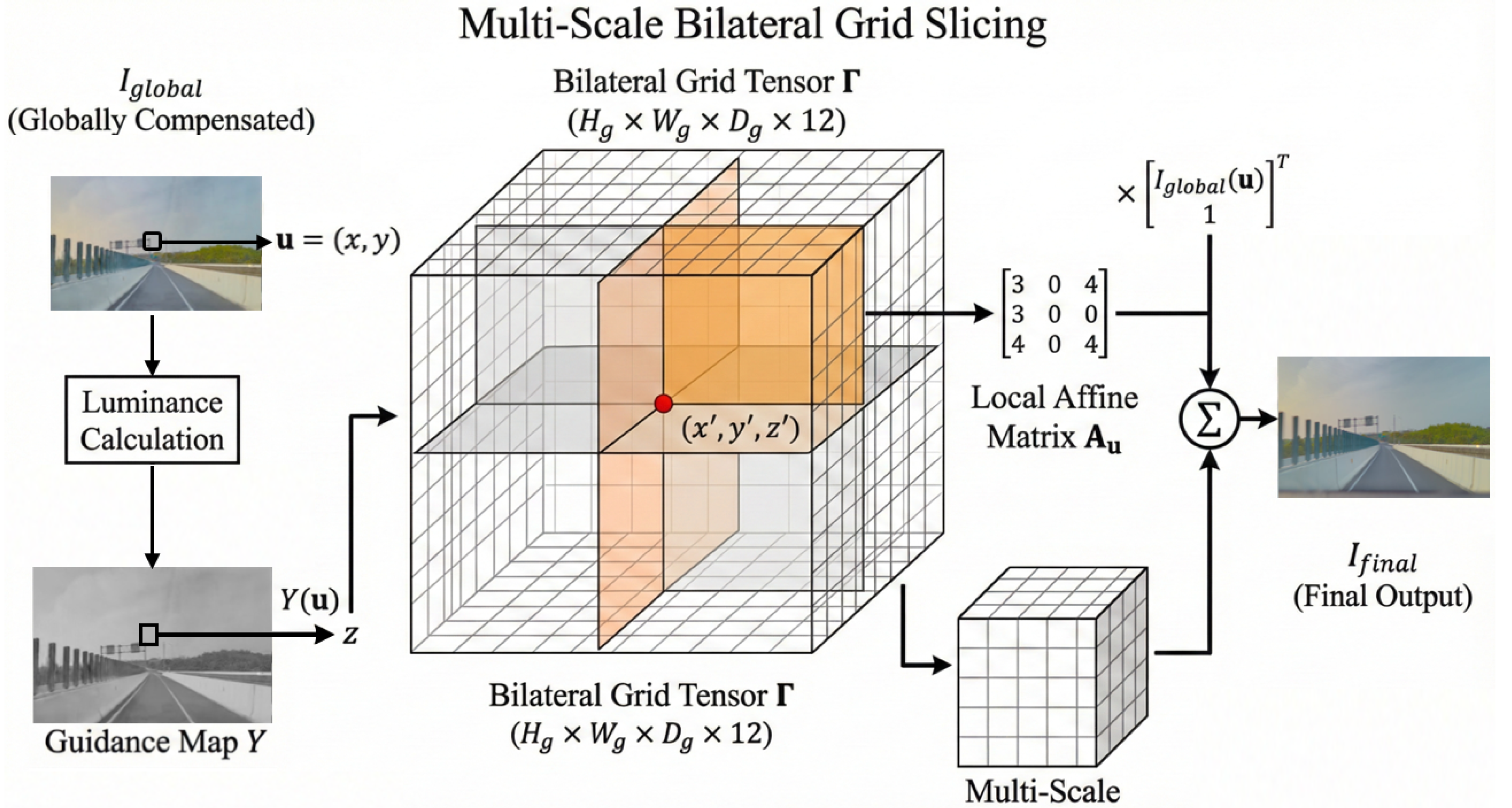
Bilateral Grid Parameterization. We parameterize the local photometric response as a learnable 3D tensor . The grid dimensions and correspond to the spatial and luminance resolutions, respectively. Each voxel stores a flattened affine transformation matrix, allowing the grid to model complex local color twists rather than simple scalar scaling.
Content-Adaptive Slicing. To enable edge-aware filtering, the correction for any given pixel is conditioned on both its spatial location and its photometric intensity. We first extract a monochromatic guidance map from the globally aligned image :
This guidance map lifts the 2D pixel coordinates into a 3D query space , where are normalized spatial coordinates and . We then retrieve a pixel-specific affine matrix via a differentiable trilinear interpolation (slicing) operator :
Multi-Scale Residual Fusion. Photometric inconsistencies often manifest at varying frequencies—vignetting is globally smooth, whereas tone-mapping artifacts can be sharp. To capture this spectrum, we employ a multi-scale hierarchy with K grid levels (typically , with resolutions and ). The final compensated image is synthesized by accumulating residual corrections:
Here, the affine matrix operates on the homogeneous representation of the pixel color. This residual formulation ensures that the grid focuses solely on local non-linear refinements, maintaining the structural fidelity of the original Gaussian rendering.
3.4. Optimization Strategy
3.4.1. Geometry-Aware SSIM-Gating
A fundamental challenge in joint geometry-appearance optimization is the texture-geometry ambiguity. Powerful appearance models (like our Multi-Scale Bilateral Grid) can easily "hallucinate" high-frequency textures or shadow artifacts to explain away photometric errors, effectively masking underlying geometric misalignments. This leads to "floating" artifacts and poor geometric convergence.
To address this, we propose a Geometry-Aware SSIM-Gated Optimization strategy, which essentially acts as a self-paced curriculum. We utilize the Structural Similarity Index (SSIM) between the raw geometry rendering (before exposure compensation) and the ground truth as a dynamic proxy for geometric reliability. We introduce a gating mask :
where is a progressive confidence threshold. During the backward pass, the gradients flowing to the exposure compensation modules (both the global affine and bilateral grid) are modulated by this mask:
where denotes the learnable parameters of the exposure modules.
- Geometric Warm-up (): When structural similarity is low, the gate is closed (). The exposure modules are effectively frozen (or reduced to identity). The optimization force focuses solely on adjusting the 3D Gaussian parameters (position, rotation, scaling) to match the scene structure using .
- Photometric Refinement (): Once the geometry is sufficiently reliable, the gate opens. The framework then jointly optimizes the exposure parameters to refine photometric alignment, correcting for sensor-specific discrepancies without corrupting the geometry.
3.4.2. Spatiotemporal Smoothness Constraints
To mitigate temporal flickering caused by independent per-frame optimization, we enforce smoothness constraints on the exposure parameters. Since auto-exposure (AE) and auto-white-balance (AWB) typically evolve smoothly over time, abrupt changes in exposure parameters between adjacent frames are penalized.
We formulate the temporal smoothness loss by decoupling it into global and local components:
where represent the affine gain and bias at time t, and represents the coefficients of the bilateral grid. The first term enforces global exposure continuity, while the second term ensures that spatially-varying corrections (e.g., vignetting patterns) remain stable over time.
3.4.3. Total Objective
The final training objective combines the standard reconstruction loss with our regularization terms:
where is a regularization term penalizing the magnitude of exposure adjustments (keeping ) to prevent color drift.
4. Experiments
4.1. Experimental Setup
4.1.1. Datasets
To validate the robustness of Lumina-4DGS under heterogeneous illumination conditions, we conduct experiments on two distinct datasets:
- 1.
- Waymo Open Dataset[27]: A large-scale driving dataset providing high-quality synchronized camera images and LiDAR point clouds. We select 5 challenging sequences (approx. 1000 frames) featuring significant lighting variations, such as strong shadows, sunlight glare, and dynamic exposure adjustments.
- 2.
- Custom Surround-View Dataset: To evaluate performance in unconstrained "in-the-wild" scenarios, we collected data using a vehicle-mounted rig of 6 cameras configured as a surround-view system. Each sensor captures high-resolution images () with independent auto-exposure (AE) and auto-white-balance (AWB) enabled. The dataset spans diverse driving conditions, including urban low-speed navigation in crowded streets, high-speed cruising on city expressways, and varying illumination from daytime to nighttime. Consequently, it is characterized by rapid inter-frame brightness shifts, severe lens vignetting, and extreme dynamic range changes, posing significant challenges for photometric consistency across the field of view.
4.1.2. Evaluation Metrics
We comprehensively evaluate the performance of Lumina-4DGS in terms of both rendering realism and geometric fidelity using the following metrics:
- Photometric Metrics: We report PSNR (↑), SSIM (↑), and LPIPS (↓). These metrics measure pixel-wise signal fidelity, structural similarity, and perceptual quality, respectively. All photometric metrics are computed between the final compensated rendering and the ground truth sensor images.
- Geometric Metric (LiDAR-based): To strictly validate the physical correctness of the reconstructed scene, we utilize LiDAR point clouds as the absolute ground truth. We evaluate the depth accuracy using RMSE (Root Mean Square Error) (↓):where is the estimated depth rendered from our Gaussian splatting model, and is the sparse but accurate ground truth depth obtained by projecting accumulated LiDAR points onto the camera image plane. denotes the set of pixels with valid LiDAR readings. This metric explicitly penalizes "floating" artifacts or geometric deformations that do not align with the physical LiDAR measurements.
4.1.3. Baselines
We compare our method against state-of-the-art view synthesis approaches:
- 3DGS[2]: The vanilla 3D Gaussian Splatting baseline.
- Street[22]: Representative dynamic urban scene reconstruction methods based on 3DGS, which model dynamic objects but typically lack explicit exposure handling mechanisms.
- OmniRe[1] A recent state-of-the-art framework that constructs hierarchical scene representations to unify static backgrounds and dynamic entities, serving as a strong baseline for holistic urban scene reconstruction.
4.1.4. Implementation Details
We implement Lumina-4DGS using PyTorch. The Multi-Scale Bilateral Grid is configured with a spatial resolution of and a luminance resolution of 8. The SSIM gating threshold is linearly annealed from to during the first 10k iterations. We train for 30k iterations on a single NVIDIA RTX 4090 GPU.
4.2. Comparative Analysis
4.2.1. Quantitative Evaluation on Public Benchmark
Table 1 summarizes the quantitative results on the Waymo Open Dataset. We compare against standard 3DGS [2], dynamic reconstruction methods Street Gaussians[22], and the recent state-of-the-art framework OmniRe [1].
Our method outperforms all baselines across photometric metrics. Notably, while Street Gaussians achieves a PSNR of 29.08 dB, and the recent OmniRe pushes the boundary to 34.61 dB, Lumina-4DGS achieves a new state-of-the-art PSNR of 35.12 dB. This represents a +0.51 dB improvement over the strongest baseline, validating the efficacy of our hierarchical exposure compensation in recovering high-fidelity details.
Crucially, regarding geometric accuracy, high photometric scores do not always correlate with correct geometry. Methods utilizing aggressive appearance embeddings (like OmniRe) can achieve high PSNR by "overfitting" texture to compensate for geometric errors. By benchmarking against LiDAR ground truth, we observe that OmniRe, while photometrically strong, yields a Depth RMSE of 2.05m. In contrast, thanks to our SSIM-Gated Optimization, Lumina-4DGS achieves the lowest Depth RMSE (1.89m). This demonstrates that our method improves visual quality through physically grounded exposure modeling rather than geometric deformation.
4.2.2. Quantitative Evaluation on Our Self-Collected "In-the-wild" Dataset
While public benchmarks like the Waymo Open Dataset provide a standardized training ground, they represent an "idealized" autonomous driving scenario. To rigorously evaluate robustness in unconstrained real-world environments, we conduct experiments on our Self-Collected Surround-View Dataset.
Unlike curated public datasets, our proprietary data was captured using a commercial sensor suite without lab-grade synchronization, introducing two distinct challenges:
- Photometric Inconsistency: Independent Auto-Exposure (AE) and Auto-White-Balance (AWB) cause drastic brightness shifts.
- LiDAR-Vision FoV Mismatch: Our setup exhibits a significant Field-of-View (FoV) gap between the cameras and the sparse LiDAR.
Quantitative Results. As shown in Table 2, this domain gap causes a "performance collapse" for state-of-the-art baselines. OmniRe [1] suffers a drastic drop (PSNR drops to 24.90 dB, LPIPS rises to 0.344). This confirms that methods relying heavily on accurate geometric initialization fail when LiDAR supervision is sparse and illumination fluctuates.
In contrast, Lumina-4DGS demonstrates remarkable robustness. By explicitly decoupling exposure from geometry and employing SSIM-Gating to handle the FoV mismatch, we achieve a PSNR of 27.23 dB (+2.33 dB over OmniRe) and a significantly lower LPIPS of 0.112 (vs. 0.344 for OmniRe).
4.2.3. Qualitative Comparison
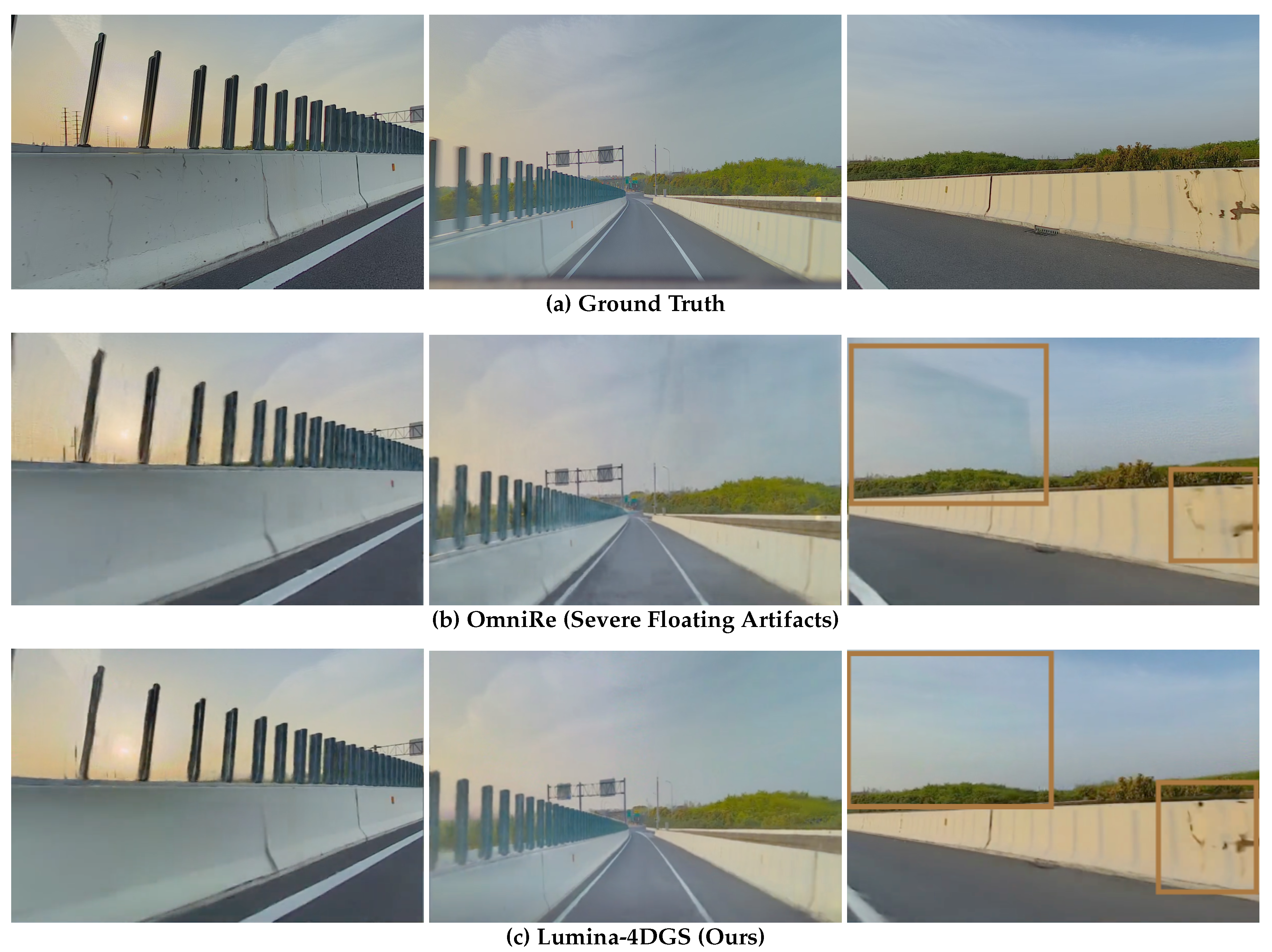
Figure 4 provides a detailed visual analysis of reconstruction quality under challenging independent auto-exposure conditions.
As evidenced in the second row, the baseline OmniRe [1] exhibits severe geometry-texture ambiguity. In the absence of LiDAR supervision for the upper field of view (e.g., sky and distant buildings), the model misinterprets rapid photometric shifts as geometric density. This leads to the hallucination of floating artifacts—manifesting as volumetric fog or haze—and results in blurred, inconsistent textures.
In contrast, Lumina-4DGS (third row) employs our SSIM-Gated mechanism to explicitly disentangle sensor dynamics from scene geometry. By penalizing erroneous density growth in photometrically unstable regions, our method suppresses these artifacts, yielding clean, temporally stable renderings that preserve geometric integrity.
4.3. Geometric Consistency and Ablation Study
A key hypothesis of our work is that unconstrained exposure optimization leads to texture-geometry ambiguity, where the model generates geometric artifacts to explain away photometric differences. To verify this and validate our design choices, we conduct a comprehensive ablation study on the Waymo dataset, evaluating the contribution of the Global Exposure Module, Multi-Scale Bilateral Grid, and SSIM-Gated Optimization.
Table 3 summarizes the quantitative results. We report both photometric metrics (PSNR, SSIM) to evaluate rendering quality and Depth RMSE (benchmarked against LiDAR) to assess geometric accuracy.
Analysis of Results:
- Global Affine Only: Adding global compensation yields a significant boost in photometric quality (PSNR: 28.15 → 30.50 dB), confirming that global sensor sensitivity shifts are the primary source of reconstruction error in auto-exposure footage.
- The Overfitting Trap (Grid w/o Gate): When the Multi-Scale Bilateral Grid is introduced without gating, the model achieves the highest photometric scores (PSNR peaks at 33.10 dB). However, this comes at the cost of geometric integrity: the Depth RMSE degrades significantly to 2.95m. This quantitative evidence, validated against LiDAR ground truth, supports our hypothesis that a powerful appearance model, if left unchecked, will "overfit" to photometric inconsistencies by deforming the scene geometry (creating artifacts to minimize RGB loss).
- Efficacy of SSIM Gating (Full Method): By enabling SSIM-Gated Optimization, we successfully resolve this ambiguity. Although there is a negligible drop in PSNR (-0.32 dB compared to the non-gated version), the geometric accuracy improves drastically (RMSE drops from 2.95m to 1.89m). This result quantitatively demonstrates that our gating strategy effectively prioritizes correct physical structure over pixel-perfect photometric overfitting, achieving the best balance between rendering quality and geometric fidelity.
5. Discussion
The experimental results presented in Section 4 demonstrate that Lumina-4DGS effectively resolves the long-standing challenge of photorealistic reconstruction under unconstrained illumination conditions. In this section, we interpret these findings in the context of previous studies, analyze the underlying mechanisms of our success, and discuss the broader implications for autonomous driving simulation.
5.1. Resolving the Texture-Geometry Ambiguity
A critical finding of our study is the confirmation of the "texture-geometry ambiguity" hypothesis. Previous state-of-the-art methods, such as OmniRe [1] and Street Gaussians [22], operate under the assumption that photometric consistency correlates directly with geometric accuracy. However, our ablation studies (Table 3) reveal that this assumption breaks down in "in-the-wild" scenarios with independent auto-exposure. When the rendering equation is forced to minimize the RGB loss against fluctuating brightness without explicit exposure decoupling, the optimizer resorts to "overfitting" by deforming the scene geometry—manifesting as the floating artifacts observed in Figure 4.
Our method fundamentally alters this optimization landscape. By introducing the Global Exposure Module, we mathematically disentangle sensor-induced sensitivity shifts from physical surface albedo. More importantly, the SSIM-Gated Optimization serves as a structural regularizer. By rejecting gradient updates in regions where structural similarity is low (indicating a transient photometric error rather than a geometric misalignment), we force the Gaussian primitives to adhere to the physical scene geometry. This explains why Lumina-4DGS maintains the lowest Depth RMSE (1.89m) even when photometrically outperforming baselines.
5.2. Bridging the Gap to Production Data
Most existing NeRF and 3DGS-based approaches are benchmarked on curated datasets like Waymo or NuScenes, which feature synchronized sensors and consistent exposure. Our experiments on the Self-Collected Surround-View Dataset highlight a significant "domain gap" between these idealized benchmarks and production-grade sensor data.
The performance collapse of baselines on our custom dataset (Table 2) underscores the fragility of current SOTA methods when facing LiDAR-Vision FoV mismatches and independent AE/AWB. Lumina-4DGS demonstrates that robust view synthesis in real-world applications requires modeling the sensor’s physical characteristics (e.g., ISO gain, vignetting) as part of the reconstruction pipeline. This capability is particularly valuable for building high-fidelity digital twins using low-cost, unsynchronized commercial fleets, significantly lowering the barrier to entry for large-scale data simulation.
5.3. Limitations and Future Directions
Despite these advancements, our current framework has limitations. First, while we effectively handle sensor-induced exposure changes, physical illumination changes caused by dynamic weather (e.g., moving cloud shadows, heavy rain, or snow) introduce complex light transport effects that our affine model cannot fully capture. Second, in regions with extreme motion blur or complete darkness, the SSIM gating mechanism may become overly conservative, potentially hindering geometry convergence.
Future research will focus on two directions: (1) integrating physics-based weather rendering models to separate environmental illumination from sensor exposure; and (2) extending our framework to an end-to-end neural sensor simulation pipeline, allowing for the synthesis of not just RGB images, but also raw sensor data with realistic noise profiles for downstream perception testing.
6. Conclusion
In this paper, we presented Lumina-4DGS, a novel framework designed to achieve illumination-robust 4D Gaussian Splatting for dynamic scene reconstruction. Addressing the limitations of existing methods in unconstrained environments, we identified the "texture-geometry ambiguity" as the primary obstacle where dynamic illumination shifts are often misinterpretation as geometric motion or structural noise.
To overcome this, we introduced a hierarchical exposure compensation pipeline integrated with a spatially-aware SSIM-Gated Optimization strategy. This approach effectively decouples sensor-induced photometric variations from the true temporal dynamics of the 4D scene. Extensive experiments on the Waymo Open Dataset and our challenging self-collected fleet dataset demonstrate that Lumina-4DGS not only achieves state-of-the-art rendering quality under rapid exposure changes but also recovers geometrically consistent structures, as validated against LiDAR ground truth.
By enabling robust reconstruction in the presence of independent auto-exposure and varying lighting conditions, Lumina-4DGS significantly closes the gap between idealized benchmarks and real-world autonomous driving data. We believe this work provides a solid foundation for creating high-fidelity, physically consistent digital twins for dynamic urban environments.
Author Contributions
Conceptualization, X.W.; methodology, X.W.; validation, X.W. and Y.S.; formal analysis, X.W. and S.L.; data curation, S.L.; writing—original draft preparation, X.W., Y.S. and S.L.; writing—review and editing, X.W. and Q.W.; supervision, Q.W.; project administration, Q.W.; funding acquisition, Q.W. All authors have read and agreed to the published version of the manuscript.
Funding
This research was funded by the National Natural Science Foundation of China, grant number 42374029.
Data Availability Statement
Publicly available datasets were analyzed in this study. The Waymo Open Dataset can be found here: https://waymo.com/open/. The self-collected dataset used in this study is not publicly available due to privacy restrictions.
Acknowledgments
We would like to thank the Waymo Open Dataset team for providing the high-quality autonomous driving data that made this research possible. We also extend our gratitude to the authors of OmniRe for open-sourcing their codebase, which served as a valuable baseline for our comparative analysis. Finally, we acknowledge the technical support provided by the DriveStudio team
Conflicts of Interest
The authors declare no conflicts of interest.
References
- Chen, Z.; Yang, J.; Huang, J.; de Lutio, R.; Martinez Esturo, J.; Ivanovic, B.; Litany, O.; Gojcic, Z.; Fidler, S.; Pavone, M.; et al. Omnire: Omni urban scene reconstruction. arXiv 2024. arXiv:2408.16760. [CrossRef]
- Kerbl, B.; Kopanas, G.; Leimkühler, T.; Drettakis, G. 3D Gaussian Splatting for Real-time Radiance Field Rendering. ACM Transactions on Graphics 2023, 42(4), 1–14. [Google Scholar] [CrossRef]
- Mildenhall, B.; Srinivasan, P. P.; Tancik, M. T.; Barron, J. T.; Ramamoorthi, R.; Ng, R. Nerf: Representing scenes as neural radiance fields for view synthesis. Communications of the ACM 2021, 65(1), 99–106. [Google Scholar] [CrossRef]
- Zhang, S.; Ye, B.; Chen, X.; Chen, Y.; Zhang, Z.; Peng, C.; Shi, Y.; Zhao, H. Drone-assisted Road Gaussian Splatting with Cross-view Uncertainty. In Proceedings of the British Machine Vision Conference (BMVC) arXiv, 2024. [Google Scholar]
- Kulhanek, J.; Peng, S.; Kukelova, Z.; Pollefeys, M.; Sattler, T. Wildgaussians: 3d gaussian splatting in the wild. arXiv 2024. arXiv:2407.08447. [CrossRef]
- Ye, S.; Dong, Z.-H.; Hu, Y.; Wen, Y.-H.; Liu, Y.-J. Gaussian in the Dark: Real-Time View Synthesis From Inconsistent Dark Images Using Gaussian Splatting. Proceedings of Pacific Graphics 2024 (PG 2024) arXiv, 2024. [Google Scholar]
- Chen, X.; Xiong, Z.; Chen, Y.; Li, G.; Wang, N.; Luo, H.; Chen, L.; Sun, H.; Wang, B.; Chen, G.; Ye, H.; Li, H.; Zhang, Y.-Q.; Zhao, H. DGGT: Feedforward 4D Reconstruction of Dynamic Driving Scenes using Unposed Images. arXiv arXiv:2512.03004. [CrossRef]
- Tonderski, A.; Lindström, C.; Hess, G.; Ljungbergh, W.; Svensson, L.; Petersson, C. Neurad: Neural rendering for autonomous driving. In Proceedings of the IEEE/CVF Conference on Computer Vision and Pattern Recognition (CVPR), 2024. [Google Scholar]
- Wang, Y.; Wang, C.; Gong, B.; Xue, T. Bilateral guided radiance field processing. ACM Transactions on Graphics (TOG) 2024, 43(4), 1–13. [Google Scholar] [CrossRef]
- Wang, P.; Liu, L.; Liu, Y.; Theobalt, C.; Komura, T.; Wang, W. Neus: Learning neural implicit surfaces by volume rendering for multi-view reconstruction. arXiv arXiv:2106.10689.
- Martin-Brualla, R.; Radwan, N.; Sajjadi, M. S. M.; Barron, J. T.; Dosovitskiy, A.; Duckworth, D. NeRF in the Wild: Neural radiance fields for unconstrained photo collections. In Proceedings of the IEEE/CVF Conference on Computer Vision and Pattern Recognition (CVPR), 2021; pp. 2–8. [Google Scholar]
- Tancik, M.; Weber, E.; Ng, E.; Li, R.; Yi, B.; Wang, T.; Kristoffersen, A.; Austin, J.; Salahi, K.; Ahuja, A.; et al. Nerfstudio: A modular framework for neural radiance field development. ACM Transactions on Graphics (TOG), 2023; 2. [Google Scholar]
- Huang, N.; Wei, X.; Zheng, W.; An, P.; Lu, M.; Zhan, W.; Tomizuka, M.; Keutzer, K.; Zhang, S. S3Gaussian: Self-Supervised Street Gaussians for Autonomous Driving. arXiv 2024. arXiv:2405.20323.
- Fischer, T.; Kulhanek, J.; Rota Bulò, S.; Porzi, L.; Pollefeys, M.; Kontschieder, P. Dynamic 3D Gaussian fields for urban areas. arXiv 2024, 3. [Google Scholar] [CrossRef]
- Fridovich-Keil, S.; Meanti, G.; Warburg, F. R.; Recht, B.; Kanazawa, A. K-Planes: Explicit radiance fields in space, time, and appearance. Proceedings of the IEEE/CVF Conference on Computer Vision and Pattern Recognition (CVPR) 2023, 2, 7, 9. [Google Scholar]
- Zhang, D.; Wang, C.; Wang, W.; Li, P.; Qin, M.; Wang, H. Gaussian in the wild: 3d gaussian splatting for unconstrained image collections. In Proceedings of the European Conference on Computer Vision (ECCV) arXiv, 2024; pp. 341–359. [Google Scholar]
- Wu, Z.; Liu, T.; Luo, L.; Zhong, Z.; Chen, J.; Xiao, H.; Hou, C.; Lou, H.; Chen, Y.; Yang, R.; et al. Mars: An instance-aware, modular and realistic simulator for autonomous driving. CAAI International Conference on Artificial Intelligence, 2023; Springer; pp. pages 3–15. [Google Scholar]
- Yuan, S.; Zhao, H. SlimmeRF: Slimmable Radiance Fields. In Proceedings of the 2024 International Conference on 3D Vision (3DV), 2024; pp. 64–74. [Google Scholar]
- Liu, H.; Jiang, P.; Huang, J.; Lu, M. Lumos3D: A Single-Forward Framework for Low-Light 3D Scene Restoration. arXiv arXiv:2511.09818.
- Wang, N.; Chen, Y.; Xiao, L.; Xiao, W.; Li, B.; Chen, Z.; Ye, C.; Xu, S.; Zhang, S.; Yan, Z.; Merriaux, P.; Lei, L.; Xue, T.; Zhao, H. Unifying Appearance Codes and Bilateral Grids for Driving Scene Gaussian Splatting. arXiv arXiv:2506.05280. [CrossRef]
- Afifi, M.; Zhao, L.; Punnappurath, A.; Abdelsalam, M. A.; Zhang, R.; Brown, M. S. Time-Aware Auto White Balance in Mobile Photography. In Proceedings of the IEEE International Conference on Computer Vision (ICCV), Honolulu, Hawaii, USA, Oct 19–23; 2025, pp. 64–74.
- Yan, Y.; Lin, H.; Zhou, C.; Wang, W.; Sun, H.; Zhan, K.; Lang, X.; Zhou, X.; Peng, S. Street Gaussians: Modeling dynamic urban scenes with gaussian splatting. In Proceedings of the European Conference on Computer Vision, 2024; Springer; pp. 156–173. [Google Scholar]
- Zhou, X.; Lin, Z.; Shan, X.; Wang, Y.; Sun, D.; Yang, M.-H. DrivingGaussian: Composite Gaussian splatting for surrounding dynamic autonomous driving scenes. In Proceedings of the IEEE/CVF Conference on Computer Vision and Pattern Recognition, 2024; pp. pages 21634–21643. [Google Scholar]
- He, L.; Li, L.; Sun, W.; Han, Z.; Liu, Y.; Zheng, S.; Wang, J.; Li, K. Neural Radiance Field in Autonomous Driving: A Survey. arXiv 2024. arXiv:2404.13816. [CrossRef]
- Du, Y.; Zhang, Y.; Yu, H.-X.; Tenenbaum, J. B.; Wu, J. Neural radiance flow for 4D view synthesis and video processing. In Proceedings of the IEEE/CVF International Conference on Computer Vision (ICCV), 2021; 2. [Google Scholar]
- Dahmani, H.; Bennehar, M.; Piasco, N.; Roldao, L.; Tsishkou, D. SWAG: Splatting in the wild images with appearance-conditioned gaussians. arXiv 2024. arXiv:2403.104273, 7, 8, 9.
- Sun, P.; Kretzschmar, H.; Dotiwalla, X.; Chouard, A.; Patnaik, V.; Tsui, P.; Guo, J.; Zhou, Y.; Chai, Y.; Caine, B.; et al. Scalability in perception for autonomous driving: Waymo open dataset. In Proceedings of the IEEE/CVF Conference on Computer Vision and Pattern Recognition (CVPR), 2020; pp. 2446–2454. [Google Scholar]
- Wilson, B.; Qi, W.; Agarwal, T.; Lambert, J.; Singh, J.; Khandelwal, S.; Pan, B.; Kumar, R.; Hartnett, A.; Pontes, J. K.; et al. Argoverse 2: Next generation datasets for self-driving perception and forecasting. arXiv 2023. arXiv:2301.00493. [CrossRef]
- Xu, B.; Xu, Y.; Yang, X.; Jia, W.; Guo, Y. Bilateral grid learning for stereo matching networks. In Proceedings of the IEEE/CVF Conference on Computer Vision and Pattern Recognition (CVPR), 2021; pp. 12497–12506. [Google Scholar]
- Liu, M.; Liu, J.; Zhang, Y.; Li, J.; Yang, M. Y.; Nex, F.; Cheng, H. 4DSTR: Advancing Generative 4D Gaussians with Spatial-Temporal Rectification for High-Quality and Consistent 4D Generation. In Proceedings of the Association for the Advancement of Artificial Intelligence (AAAI) arXiv, 2025. [Google Scholar]
- Guédon, A.; Lepetit, V. Sugar: Surface-aligned gaussian splatting for efficient 3d mesh reconstruction and high-quality mesh rendering. arXiv 2023. arXiv:2311.12775.
- Jiang, Y.; Tu, J.; Liu, Y.; Gao, X.; Long, X.; Wang, W.; Ma, Y. GaussianShader: 3D Gaussian Splatting with Shading Functions for Reflective Surfaces. arXiv 2023. arXiv:2311.17977. [CrossRef]
- Fu, C.; Chen, G.; Zhang, Y.; Yao, K.; Xiong, Y.; Huang, C.; Cui, S.; Matsushita, Y.; Cao, X. RobustSplat++: Decoupling Densification, Dynamics, and Illumination for In-the-Wild 3DGS. arXiv arXiv:2512.04815.
- Huang, B.; Yu, Z.; Chen, A.; Geiger, A.; Gao, S. 2D Gaussian Splatting for Geometrically Accurate Radiance Fields. ACM SIGGRAPH 2024 Conference Papers, 2024; pp. 1–11. [Google Scholar]
- Huang, X.; Li, J.; Wu, T.; Zhou, X.; Han, Z.; Gao, F. Flying in Clutter on Monocular RGB by Learning in 3D Radiance Fields with Domain Adaptation. In Proceedings of the 2025 IEEE International Conference on Robotics and Automation (ICRA) 2025 arXiv, 2025. [Google Scholar]
- Wang, J.; Che, H.; Chen, Y.; Yang, Z.; Goli, L.; Manivasagam, S.; Urtasun, R. Flux4D: Flow-based Unsupervised 4D Reconstruction. arXiv arXiv:2512.03210.
- Huang, Y.; Bai, L.; Cui, B.; Li, Y.; Chen, T.; Wang, J.; Wu, J.; Lei, Z.; Liu, H.; Ren, H. Endo-4DGX: Robust Endoscopic Scene Reconstruction and Illumination Correction with Gaussian Splatting. In Proceedings of the 2025 International Conference on Medical Image Computing and Computer Assisted Intervention (MICCAI) 2025 arXiv, 2025. [Google Scholar]
- Wei, X.; Ye, Z.; Gu, Y.; Zhu, Z.; Guo, Y.; Shen, Y.; Zhao, S.; Lu, M.; Sun, H.; Wang, B.; Chen, G.; Lu, R.; Ye, H. ParkGaussian: Surround-view 3D Gaussian Splatting for Autonomous Parking. arXiv 2026. arXiv:2601.01386.
Figure 1.
Overview of the Lumina-4DGS Framework.The scene is modeled via a composite Gaussian Scene Graph and rendered to produce a raw image . (Middle) A Hierarchical Exposure Compensation stage normalizes using a Global Exposure Module for sensor-level shifts () and a Multi-Scale Bilateral Grid for local non-linearities, yielding the final image . (Right) Optimization is controlled by an SSIM-Gated Mechanism, which enforces temporal smoothness and dynamically gates gradient flow to ensure appearance enhancements do not compromise geometric structural reliability.
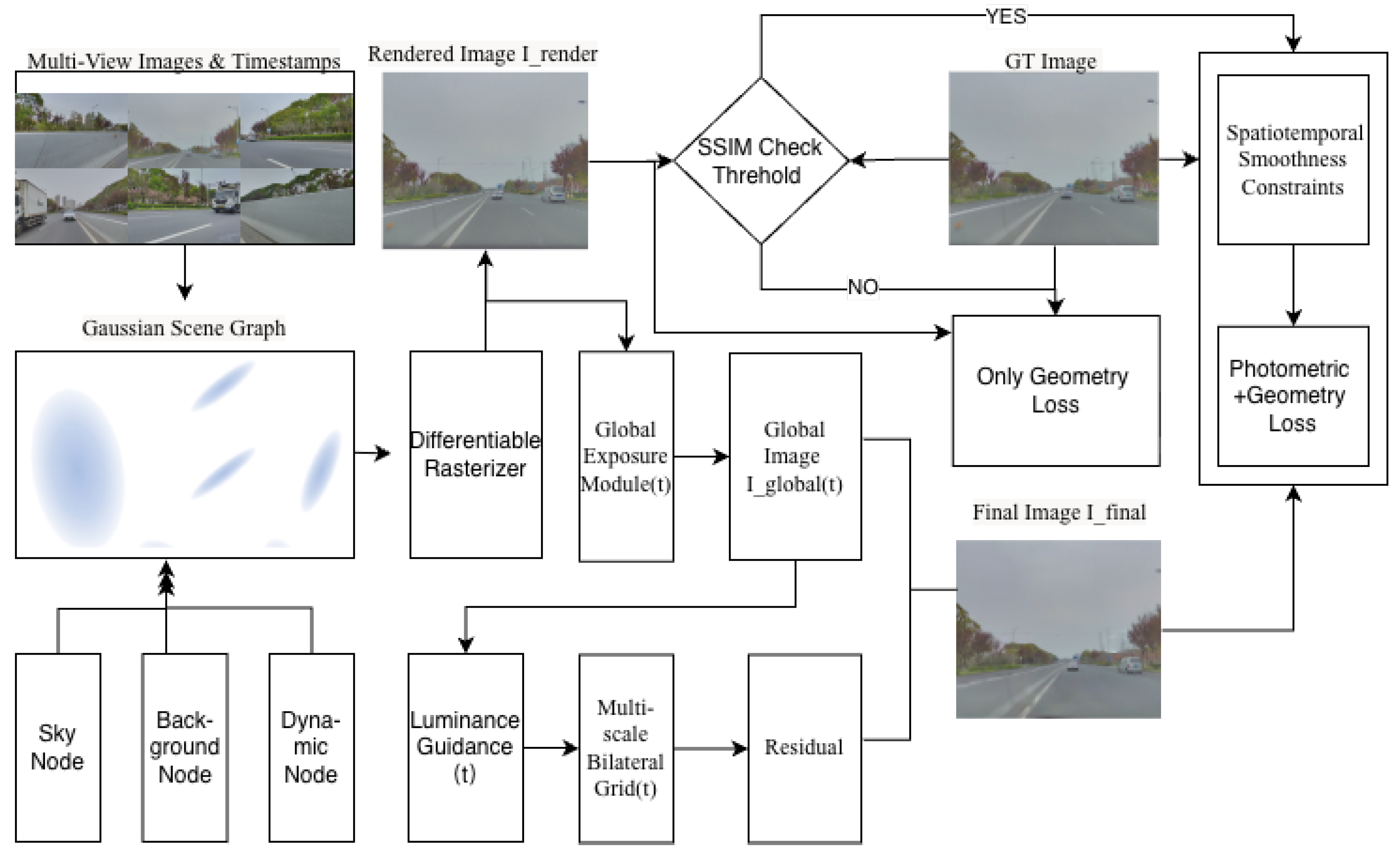
Figure 2.
Scene Graph Decomposition based on Semantic Priors. We utilize off-the-shelf segmentation models to decouple the scene into three semantic primitives: Sky Node (, blue), Dynamic Node (, red), and Background Node (, gray). This decomposition initializes our graph structure, enabling specific kinematic constraints for each node type.
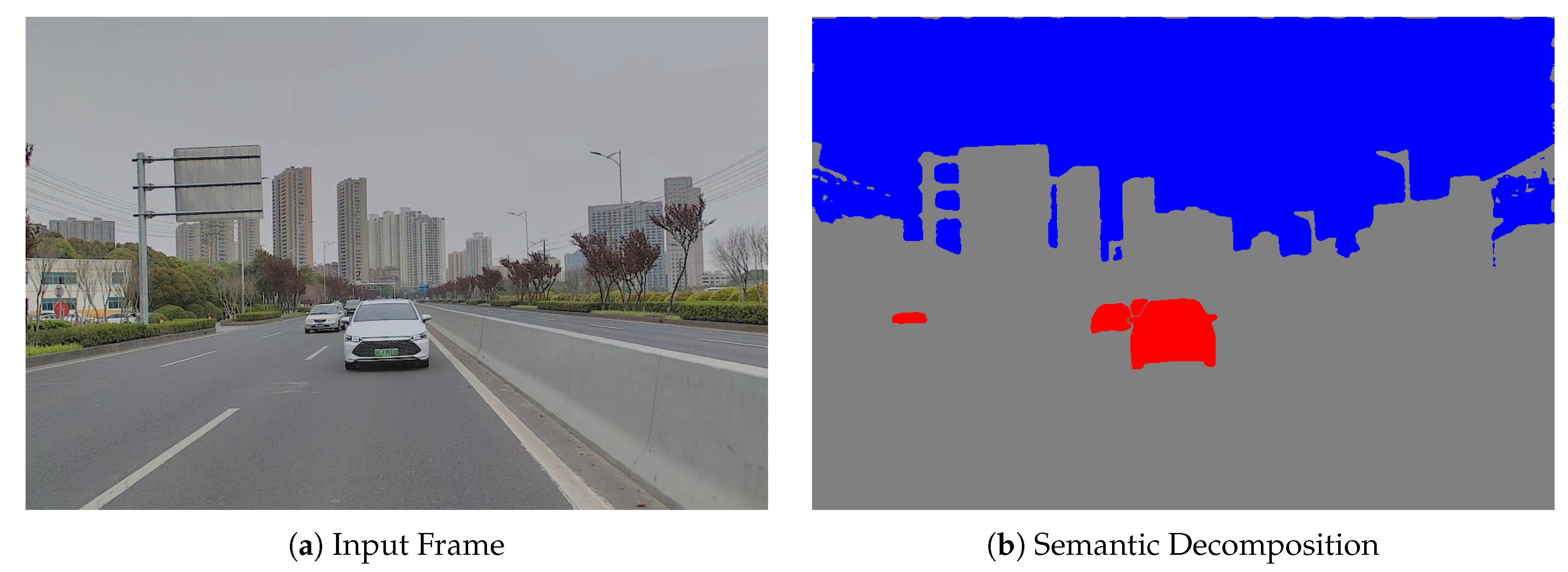
Figure 4.
Visualizing the impact of exposure inconsistency on geometric reconstruction. (a) Ground Truth frames captured with independent AE/AWB, showing significant brightness shifts. (b) OmniRe fails to decouple illumination from geometry. Lacking LiDAR constraints in the sky, it overfits to brightness changes by generating floating artifacts (visible as hazy noise) to minimize photometric error. (c) Lumina-4DGS (Ours) effectively harmonizes exposure and enforces structural integrity via SSIM-gating, successfully removing these artifacts to produce sharp, clean renderings.
| (a) Ground Truth | ||
| (b) OmniRe (Severe Floating Artifacts) | ||
| (c) Lumina-4DGS (Ours) | ||

Table 1.
Quantitative comparison on Waymo Open Dataset. Best results are bolded, second best are underlined. Note that our method achieves superior rendering quality (PSNR) while maintaining the most accurate geometry (RMSE validated against LiDAR).
Table 1.
Quantitative comparison on Waymo Open Dataset. Best results are bolded, second best are underlined. Note that our method achieves superior rendering quality (PSNR) while maintaining the most accurate geometry (RMSE validated against LiDAR).
| Method | Photometric Quality | Geometric Quality | ||
|---|---|---|---|---|
| PSNR ↑ | SSIM ↑ | LPIPS ↓ | Depth RMSE (m)↓ | |
| 3DGS[2] | 26.00 | 0.918 | 0.117 | 2.80 |
| Street Gaussians [22] | 29.08 | 0.936 | 0.125 | 2.20 |
| OmniRe [45] | 34.61 | 0.938 | 0.079 | 2.05 |
| Lumina-4DGS (Ours) | 35.12 | 0.956 | 0.072 | 1.89 |
Table 2.
Quantitative comparison on Our Self-Collected Dataset. This proprietary dataset features severe AE/AWB shifts and large LiDAR-Vision FoV gaps. Lumina-4DGS maintains superior structural (SSIM) and perceptual (LPIPS) quality.
Table 2.
Quantitative comparison on Our Self-Collected Dataset. This proprietary dataset features severe AE/AWB shifts and large LiDAR-Vision FoV gaps. Lumina-4DGS maintains superior structural (SSIM) and perceptual (LPIPS) quality.
| Method | PSNR ↑ | SSIM ↑ | LPIPS ↓ |
|---|---|---|---|
| 3DGS [2] | 23.15 | 0.765 | 0.385 |
| Street Gaussians [22] | 23.82 | 0.772 | 0.368 |
| OmniRe [45] | 24.90 | 0.796 | 0.344 |
| Lumina-4DGS (Ours) | 27.23 | 0.811 | 0.112 |
Table 3.
Ablation study evaluating the contribution of each component. Global: Global Exposure Module. Grid: Multi-Scale Bilateral Grid. Gate: SSIM-Gated Optimization. Note the trade-off between photometric fitting and geometric integrity in the third row.
Table 3.
Ablation study evaluating the contribution of each component. Global: Global Exposure Module. Grid: Multi-Scale Bilateral Grid. Gate: SSIM-Gated Optimization. Note the trade-off between photometric fitting and geometric integrity in the third row.
| Components | Photometry | Geometry | |||
|---|---|---|---|---|---|
| Global | Grid | Gate | PSNR ↑ | SSIM ↑ | Depth RMSE↓ |
| - | - | - | 28.15 | 0.852 | 2.80 |
| √ | - | - | 30.50 | 0.880 | 2.75 |
| √ | √ | - | 33.10 | 0.920 | 2.95 (Degraded) |
| √ | √ | √ | 32.78 | 0.915 | 1.89(Restored) |
Disclaimer/Publisher’s Note: The statements, opinions and data contained in all publications are solely those of the individual author(s) and contributor(s) and not of MDPI and/or the editor(s). MDPI and/or the editor(s) disclaim responsibility for any injury to people or property resulting from any ideas, methods, instructions or products referred to in the content. |
© 2026 by the authors. Licensee MDPI, Basel, Switzerland. This article is an open access article distributed under the terms and conditions of the Creative Commons Attribution (CC BY) license (http://creativecommons.org/licenses/by/4.0/).
Copyright: This open access article is published under a Creative Commons CC BY 4.0 license, which permit the free download, distribution, and reuse, provided that the author and preprint are cited in any reuse.


