Electromagnetic Back-Action in Dipole–Loop Magnetomechanics: State–Space Model, Memory Kernel, and Jerk/Absement Asymptotes

1. Introduction

Magnet–conductor and magnet–superconductor interactions are central to magnetic damping, eddy-current brakes, inductive sensing, levitation, and magnetomechanical devices. In many reduced-order mechanical models, magnetic effects are represented as either (i) conservative stiffness (from magnetostatics) or (ii) viscous damping (from induced currents). However, Maxwell–Faraday induction with finite circuit inductance implies a history-dependent back-action force whose effective stiffness and loss vary with frequency [1,2,3,4].

Goal and scope.

We treat a permanent magnet as a point dipole and focus on 1D axial motion relative to a single loop/coil. This is the minimal setting that: (i) is derivable directly from Maxwell–Faraday induction, (ii) yields a causal memory kernel with a single relaxation time, and (iii) produces clear, testable dynamic-stiffness and dissipation signatures.

Main contributions.

Within this minimal magnetomechanical system we provide:

1.

an energy-consistent state–space model for magnet motion coupled to an RL loop;

2.

an exact complex dynamic stiffness and its decomposition into added stiffness and added damping;

3.

a Maxwell-element equivalence (spring–dashpot series) guaranteeing passivity and offering mechanical intuition [6];

4.

closed-form identification formulas for $(\tau ,k_{\infty })$ from complex stiffness data;

5.

a geometry-based design rule: $|{\mathsf{\Lambda }}^{\prime }\left(x_0\right)|$ is maximized at $x_0=a/2$;

6.

a controlled interpretation of “jerk” and “absement” as asymptotes of the same passive memory element (not ad hoc constitutive laws).

2. Dipole Flux and Flux-Linkage Gradient

2.1. Geometry and Dipole Approximation

Consider a magnetic dipole moment $\mathbf{m}=m\widehat{\mathbf{z}}$ located on the symmetry axis of a circular loop of radius a lying in the plane $z=0$. Let $x\left(t\right)$ denote the dipole’s axial position measured from the loop center (so $x>0$ is “above” the loop). The dipole approximation is appropriate when distances are large compared to magnet dimensions [1,2].

2.2. Flux via Vector Potential

For a dipole $\mathbf{m}=m\widehat{\mathbf{z}}$ at the origin, the azimuthal component of the vector potential in cylindrical coordinates $(\rho ,\phi ,z)$ is [1]

$$A_{\phi }(\rho ,z)={\displaystyle \frac{{\mu }_{0}m\rho }{4\pi {({\rho }^2+z^2)}^{3/2}}}.$$

(1)

For a loop of radius a at axial offset x, the flux through one turn is obtained by $\mathsf{\Phi }=\oint \mathit{A}·d\ell =2\pi a{A}_{\phi }(a,x)$:

$$\mathsf{\Phi }\left(x\right)={\displaystyle \frac{{\mu }_{0}m{a}^2}{2{(a^2+x^2)}^{3/2}}}.$$

(2)

Its derivative is

$${\mathsf{\Phi }}^{\prime }\left(x\right)=\mathsf{\Phi }x=-{\displaystyle \frac{3{\mu }_{0}m{a}^{2}x}{2{(a^2+x^2)}^{5/2}}}.$$

(3)

2.3. Flux Linkage for an N-Turn Loop

For an N-turn loop/coil, the flux linkage (Weber-turns) is

$$\mathsf{\Lambda }\left(x\right)=N\mathsf{\Phi }\left(x\right),{\mathsf{\Lambda }}^{\prime }\left(x\right)=N{\mathsf{\Phi }}^{\prime }\left(x\right).$$

(4)

2.4. Scaling Laws and Optimal Operating Point

The electromechanical coupling enters through the gradient

$$G\left(x_0\right)\equiv {\mathsf{\Lambda }}^{\prime }\left(x_0\right)=N{\mathsf{\Phi }}^{\prime }\left(x_0\right).$$

Using , the explicit dipole–loop coupling gradient is

$$G\left(x_0\right)=-{\displaystyle \frac{3{\mu }_{0}mN{a}^2{x}_0}{2{(a^2+x_0^2)}^{5/2}}}.$$

(5)

Thus $\left|G\right|$ scales linearly with m and N and depends on geometry through the dimensionless ratio $x_0/a$.

Optimal operating point.

Define $t\equiv x_0/a$ and

$$g\left(t\right)\equiv {\displaystyle \frac{t}{{(1+t^2)}^{5/2}}},\left|G\left(x_0\right)\right|={\displaystyle \frac{3{\mu }_0\left|m\right|N}{2a^2}}g\left({\displaystyle \frac{x_0}{a}}\right).$$

Differentiating,

$$g^{\prime }\left(t\right)={\displaystyle \frac{1-4t^2}{{(1+t^2)}^{7/2}}},$$

so the maximum occurs at $t^{★}=1/2$. Therefore,

$$\begin{array}{|c|}\hline x_0^{★}={\displaystyle \frac{a}{2}}\\ \hline\end{array}$$

(6)

maximizes $\left|G\right|$ and, consequently, maximizes the measurable back-action signatures derived below (added stiffness and added damping) within the dipole approximation.

3. Coupled State–Space Model: Mechanics + Circuit

3.1. Circuit Equation (Faraday + Ohm + Inductance)

For an isolated loop with resistance R and inductance L, the flux linkage through the loop is

$$\lambda \left(t\right)=Li\left(t\right)+\mathsf{\Lambda }\left(x\right(t\left)\right).$$

(7)

Faraday’s law gives the induced electromotive force $-\dot{\lambda }$. With loop voltage $Ri$,

$$Ri\left(t\right)=-\lambda t=-L\dot{i}\left(t\right)-{\mathsf{\Lambda }}^{\prime }\left(x\left(t\right)\right)\dot{x}\left(t\right),$$

(8)

or equivalently

$$L\dot{i}+Ri=-{\mathsf{\Lambda }}^{\prime }\left(x\right)\dot{x}.$$

(9)

3.2. Electromagnetic Force

Using magnetic co-energy (or standard electromechanical transduction arguments), the axial electromagnetic force is

$$F_{\mathrm{em}}\left(t\right)=i\left(t\right){\mathsf{\Lambda }}^{\prime }\left(x\left(t\right)\right).$$

(10)

The sign is determined by ${\mathsf{\Lambda }}^{\prime }\left(x\right)$ and $i\left(t\right)$; Lenz’s law is enforced automatically through Equation (9).

3.3. Mechanical Equation and Full State–Space Form

To obtain bounded motion and enable frequency-domain validation, we consider a 1D mass–spring–damper with an external drive $F_{\mathrm{drv}}\left(t\right)$:

$$M\ddot{x}+c_m\dot{x}+k_m(x-x_0)=F_{\mathrm{em}}\left(t\right)+F_{\mathrm{drv}}\left(t\right),$$

(11)

with $x_0$ a chosen operating point.

The full coupled system is a state–space ODE for $\mathbf{z}=(x,v,i)$:

$$\begin{array}{cc}\hfill \dot{x}& =v,\hfill \end{array}$$

(12)

$$\begin{array}{cc}\hfill M\dot{v}& =-c_{m}v-k_m(x-x_0)+i{\mathsf{\Lambda }}^{\prime }\left(x\right)+F_{\mathrm{drv}}\left(t\right),\hfill \end{array}$$

(13)

$$\begin{array}{cc}\hfill L\dot{i}& =-Ri-{\mathsf{\Lambda }}^{\prime }\left(x\right)v.\hfill \end{array}$$

(14)

3.4. Energy Identity and Passivity

Define the total stored energy as

$$E\left(t\right)={\displaystyle \frac{1}{2}}Mv{\left(t\right)}^2+{\displaystyle \frac{1}{2}}{k}_m{(x\left(t\right)-x_0)}^2+{\displaystyle \frac{1}{2}}Li{\left(t\right)}^2.$$

(15)

Multiplying Equation (11) by v and Equation (9) by i and adding yields the power balance

$$\dot{E}\left(t\right)=-c_{m}v{\left(t\right)}^2-Ri{\left(t\right)}^2+v\left(t\right)F_{\mathrm{drv}}\left(t\right).$$

(16)

Thus the electromagnetic coupling transfers energy between mechanical and inductive storage, while the resistor dissipates $R{i}^2$. For $F_{\mathrm{drv}}=0$ and $c_m\ge 0$, $R\ge 0$, the system is passive.

4. Linearization and Frequency-Domain Response

4.1. Linearization at an Operating Point

For small oscillations about $x_0$, set

$$x\left(t\right)=x_0+\xi \left(t\right),\left|\xi \right|\ll x_0,$$

and approximate ${\mathsf{\Lambda }}^{\prime }\left(x\right)\approx {\mathsf{\Lambda }}^{\prime }\left(x_0\right)\equiv G$. Then

$$L\dot{i}+Ri=-G\dot{\xi },F_{\mathrm{em}}\left(t\right)=Gi\left(t\right),$$

(17)

and the electromechanical coupling becomes linear time-invariant.

4.2. Exact Causal Memory Kernel

Solving the first-order circuit equation gives (for $t\ge 0$)

$$i\left(t\right)=e^{-t/\tau }i\left(0\right)-{\displaystyle \frac{G}{L}}{\int }_0^t{e}^{-(t-t^{\prime })/\tau }\dot{\xi }\left(t^{\prime }\right)d{t}^{\prime },\tau \equiv {\displaystyle \frac{L}{R}}.$$

(18)

Hence the electromagnetic force is

$$F_{\mathrm{em}}\left(t\right)=G{e}^{-t/\tau }i\left(0\right)-{\displaystyle \frac{G^2}{L}}{\int }_0^t{e}^{-(t-t^{\prime })/\tau }\dot{\xi }\left(t^{\prime }\right)d{t}^{\prime }.$$

(19)

This is a history-dependent force: an exponential convolution of velocity.

4.3. Complex Dynamic Stiffness

For harmonic motion $\xi \left(t\right)=\Re \left[X{e}^{i\omega t}\right]$ and $F_{\mathrm{em}}\left(t\right)=\Re \left[F{e}^{i\omega t}\right]$, Equation (17) gives

$$(R+i\omega L)I=-i\omega GX,F=GI.$$

(20)

Define the complex dynamic stiffness as

$$K_{\mathrm{em}}\left(\omega \right)\equiv -{\displaystyle \frac{F}{X}}={\displaystyle \frac{G^{2}i\omega }{R+i\omega L}}.$$

(21)

In terms of the asymptotic stiffness scale

$$k_{\infty }\equiv {\displaystyle \frac{G^2}{L}},$$

(22)

and the time constant $\tau =L/R$, Equation (21) becomes

$${\displaystyle \frac{K_{\mathrm{em}}\left(\omega \right)}{k_{\infty }}}={\displaystyle \frac{i\omega \tau }{1+i\omega \tau }}.$$

(23)

Let $\chi \equiv \omega \tau$. Then

$$\Re \left({\displaystyle \frac{K_{\mathrm{em}}}{k_{\infty }}}\right)={\displaystyle \frac{{\chi }^2}{1+{\chi }^2}},\Im \left({\displaystyle \frac{K_{\mathrm{em}}}{k_{\infty }}}\right)={\displaystyle \frac{\chi }{1+{\chi }^2}}.$$

(24)

4.4. Exact Time-Domain Constitutive Law (Fundamental) and Internal-State Form

The asymptotic expansions in Section 5 are useful for intuition, but they are not fundamental force laws: truncations are valid only in their corresponding limits and can break passivity if applied outside them. In contrast, the linearized dipole–loop coupling admits an exact and local-in-time constitutive equation for $F_{\mathrm{em}}$.

From Equation (17), eliminate $i=F_{\mathrm{em}}/G$ to obtain

$$L{\dot{F}}_{\mathrm{em}}+R{F}_{\mathrm{em}}=-G^2\dot{\xi }.$$

(25)

Define

$$\tau \equiv {\displaystyle \frac{L}{R}},k_{\infty }\equiv {\displaystyle \frac{G^2}{L}},c_0\equiv {\displaystyle \frac{G^2}{R}}=k_{\infty }\tau .$$

(26)

Then

$${\dot{F}}_{\mathrm{em}}+{\displaystyle \frac{1}{\tau }}{F}_{\mathrm{em}}=-k_{\infty }\dot{\xi }.$$

(27)

In Laplace-domain operator form (s the Laplace variable),

$$F_{\mathrm{em}}\left(s\right)=-k_{\infty }{\displaystyle \frac{s}{s+1/\tau }}\mathsf{\Xi }\left(s\right),K_{\mathrm{em}}\left(s\right)=k_{\infty }{\displaystyle \frac{s}{s+1/\tau }},$$

(28)

which reduces to Equation (23) on $s=i\omega$.

Leaky-absement internal state (bounded memory).

Define an exponentially weighted (leaky) absement-like state

$$A\left(t\right)\equiv {\int }_0^t{e}^{-(t-t^{\prime })/\tau }\xi \left(t^{\prime }\right)d{t}^{\prime }.$$

(29)

Then

$$\dot{A}=\xi -{\displaystyle \frac{1}{\tau }}A,$$

(30)

and (after transients decay) the force may be written compactly as

$$F_{\mathrm{em}}\left(t\right)\approx -k_{\infty }\xi \left(t\right)+{\displaystyle \frac{k_{\infty }}{\tau }}A\left(t\right).$$

(31)

This internal-state representation is exact for the linearized model (up to an exponentially decaying transient term) and provides a well-posed “absement-like” variable that remains bounded for bounded $\xi$.

4.5. Added Stiffness and Added Damping; Maxwell-Element Equivalence

Write

$$K_{\mathrm{em}}\left(\omega \right)=K^{\prime }\left(\omega \right)+i{K}^{\prime \prime }\left(\omega \right).$$

A common mechanical interpretation is to define the added stiffness and added damping via

$$K_{\mathrm{em}}\left(\omega \right)=k_{\mathrm{add}}\left(\omega \right)+i\omega c_{\mathrm{add}}\left(\omega \right),k_{\mathrm{add}}\left(\omega \right)=K^{\prime }\left(\omega \right),c_{\mathrm{add}}\left(\omega \right)={\displaystyle \frac{K^{\prime \prime }\left(\omega \right)}{\omega }}.$$

From Equation (24), with $\chi =\omega \tau$,

$$\begin{array}{cc}\hfill k_{\mathrm{add}}\left(\omega \right)& =k_{\infty }{\displaystyle \frac{{\chi }^2}{1+{\chi }^2}},\hfill \end{array}$$

(32)

$$\begin{array}{cc}\hfill c_{\mathrm{add}}\left(\omega \right)& =k_{\infty }\tau {\displaystyle \frac{1}{1+{\chi }^2}}={\displaystyle \frac{c_0}{1+{\chi }^2}}.\hfill \end{array}$$

(33)

Thus the back-action behaves as: (i) predominantly viscous ($c_{\mathrm{add}}\approx c_0$) for $\omega \tau \ll 1$; and (ii) predominantly elastic ($k_{\mathrm{add}}\approx k_{\infty }$) for $\omega \tau \gg 1$.

Maxwell-element equivalence.

The Laplace-domain stiffness Equation (28) has the form

$$K_{\mathrm{em}}\left(s\right)=k_{\infty }{\displaystyle \frac{\tau s}{1+\tau s}},$$

which is identical to the dynamic stiffness of a Maxwell viscoelastic element: a spring of stiffness $k_{\infty }$ in series with a dashpot of coefficient $c_0=k_{\infty }\tau$ [6]. This provides an immediate passivity guarantee and a useful mechanical analogue: the resistor dissipates energy (dashpot-like low-frequency behavior), while the inductor stores energy (spring-like high-frequency behavior).

4.6. Direct Identification of $\tau$ and $k_{\infty }$ from Complex Stiffness

Because Equation (24) depends only on $\chi =\omega \tau$ and $k_{\infty }$, the parameters $(\tau ,k_{\infty })$ can be identified directly from measured complex stiffness data.

Let $K_{\mathrm{em}}\left(\omega \right)=K^{\prime }\left(\omega \right)+i{K}^{\prime \prime }\left(\omega \right)$ for $\omega >0$. Then

$$\begin{array}{|c|}\hline \omega \tau ={\displaystyle \frac{K^{\prime }\left(\omega \right)}{K^{\prime \prime }\left(\omega \right)}}\\ \hline\end{array}⟹\begin{array}{|c|}\hline \tau ={\displaystyle \frac{1}{\omega }}{\displaystyle \frac{K^{\prime }\left(\omega \right)}{K^{\prime \prime }\left(\omega \right)}}.\\ \hline\end{array}$$

(34)

Eliminating $\chi$ also yields

$$\begin{array}{|c|}\hline k_{\infty }={\displaystyle \frac{K^{\prime }{\left(\omega \right)}^2+K^{\prime \prime }{\left(\omega \right)}^2}{K^{\prime }\left(\omega \right)}}\\ \hline\end{array}\mathrm{and}\begin{array}{|c|}\hline c_0=k_{\infty }\tau .\\ \hline\end{array}$$

(35)

These identities provide a direct route to parameter extraction from impedance or dynamic-stiffness measurements.

5. Asymptotic Expansions: Jerk and Absement Limits

The exact memory force Equation (19) (or equivalently the exact constitutive law Equation (27)) is passive and well posed. However, it is often useful to approximate it by local derivative operators in a low-frequency regime, or by inverse-derivative (integral) operators in a high-frequency regime. We make these connections explicit and state validity constraints.

5.1. Low-Frequency Expansion (Derivative / Jerk Correction)

For $\chi =\omega \tau \ll 1$, expand Equation (23):

$${\displaystyle \frac{K_{\mathrm{em}}}{k_{\infty }}}=i\chi +{\chi }^2-i{\chi }^3-{\chi }^4+O\left({\chi }^5\right).$$

(36)

In time-domain operator language (replace $i\omega \mapsto d/dt$), the corresponding force expansion is

$$F_{\mathrm{em}}\left(t\right)\approx -{\displaystyle \frac{G^2}{R}}\dot{\xi }+{\displaystyle \frac{G^{2}L}{R^2}}\ddot{\xi }-{\displaystyle \frac{G^2{L}^2}{R^3}}\stackrel{⃛}{\xi }+\dots .$$

(37)

The third derivative term is an explicit jerk correction. Truncating Equation (37) beyond its range of validity ($\omega \tau \ll 1$) can break passivity, so it should be used only as an asymptotic approximation.

5.2. High-Frequency Expansion (Absement-Like Asymptote)

For $\chi =\omega \tau \gg 1$, expand Equation (23) as a series in $1/\chi$:

$${\displaystyle \frac{K_{\mathrm{em}}}{k_{\infty }}}={\displaystyle \frac{i\chi }{1+i\chi }}=1-{\displaystyle \frac{1}{i\chi }}+{\displaystyle \frac{1}{{\left(i\chi \right)}^2}}-{\displaystyle \frac{1}{{\left(i\chi \right)}^3}}+O\left({\chi }^{-4}\right).$$

(38)

Equivalently, in Laplace form Equation (28), for $\left|s\right|\tau \gg 1$,

$$K_{\mathrm{em}}\left(s\right)=k_{\infty }{\displaystyle \frac{s}{s+1/\tau }}=k_{\infty }\left[1-{\displaystyle \frac{1}{s\tau }}+{\displaystyle \frac{1}{{\left(s\tau \right)}^2}}-{\displaystyle \frac{1}{{\left(s\tau \right)}^3}}+\dots \right].$$

(39)

Since $F_{\mathrm{em}}\left(s\right)=-K_{\mathrm{em}}\left(s\right)\mathsf{\Xi }\left(s\right)$ by definition, the leading high-frequency time-domain approximation is

$$F_{\mathrm{em}}\left(t\right)\approx -k_{\infty }\xi \left(t\right)+{\displaystyle \frac{k_{\infty }}{\tau }}\underset{{\displaystyle B\left(t\right)}}{\underbrace{{\int }_0^t\xi \left(t^{\prime }\right)d{t}^{\prime }}}+O\left({\left(\omega \tau \right)}^{-2}\right),$$

(40)

where $B\left(t\right)$ is the (non-leaky) absement of the small displacement $\xi$ about the operating point.

Important note (why this is not fundamental).

The raw integral $B\left(t\right)={\int }_0^t\xi \left(t^{\prime }\right)d{t}^{\prime }$ can drift under DC offsets and is therefore best interpreted as an asymptotic representation for oscillatory motions with zero mean and $\omega \tau \gg 1$. For general signals and to preserve boundedness and passivity, the exact internal-state form (leaky absement) should be used.

6. Resistive Loss Under Prescribed Harmonic Motion

Assume prescribed harmonic displacement $\xi \left(t\right)=Xsin\omega t$ in the linear regime. The current amplitude from Equation (17) is

$$I_0={\displaystyle \frac{\left|G\right|\omega X}{\sqrt{R^2+{\omega }^2{L}^2}}}.$$

(41)

The cycle-averaged resistive loss is

$$\langle P_R\rangle ={\displaystyle \frac{1}{2}}R{I}_0^2={\displaystyle \frac{1}{2}}{\displaystyle \frac{G^{2}R{\omega }^2{X}^2}{R^2+{\omega }^2{L}^2}}.$$

(42)

This exhibits two asymptotic regimes:

$$\begin{array}{cc}\hfill \omega \tau \ll 1:\langle P_R\rangle & \approx {\displaystyle \frac{1}{2}}{\displaystyle \frac{G^2}{R}}{\omega }^2{X}^2\propto {\omega }^2,\hfill \end{array}$$

(43)

$$\begin{array}{cc}\hfill \omega \tau \gg 1:\langle P_R\rangle & \approx {\displaystyle \frac{1}{2}}{\displaystyle \frac{G^{2}R}{L^2}}{X}^2(\mathrm{frequency}-\mathrm{independent}\mathrm{plateau}).\hfill \end{array}$$

(44)

6.0.0.7. Remark.

The scaling here is for prescribed displacement amplitude X. Under alternative experimental constraints (e.g. prescribed drive force), observed frequency scaling can differ; Equation (21) provides the appropriate transfer function for those cases.

7. Numerical Methods and Reproducibility

All figures and datasets in this manuscript are generated using a single Python script (magnet_loop_backaction.py) using numpy, scipy, and matplotlib. The script produces:

• $\mathsf{\Phi }\left(x\right)$ and ${\mathsf{\Phi }}^{\prime }\left(x\right)$ for the dipole–loop geometry ();
• normalized $K_{\mathrm{em}}\left(\omega \right)/k_{\infty }$ and its low/high-frequency asymptotes ();
• $\langle P_R\rangle$ vs frequency and its asymptotes (Equation (42));
• time-domain ring-down simulations of the full nonlinear state–space model 12 and numerical verification of Equation (16).

The numerical example parameters used to generate the figures in Section 8 are listed in Table 1.

8. Results

8.1. Example Parameters and Derived Back-Action Scales

For these parameters, $x_0/a\simeq 0.67$. The optimal point Equation (6) would be $x_0^{★}=a/2=0.015m$, which would increase $\left|G\right|$ (and thus $k_{\infty }$ and $c_0$) by approximately $7.7\%$ relative to the present choice.

8.2. Flux and Coupling Gradient

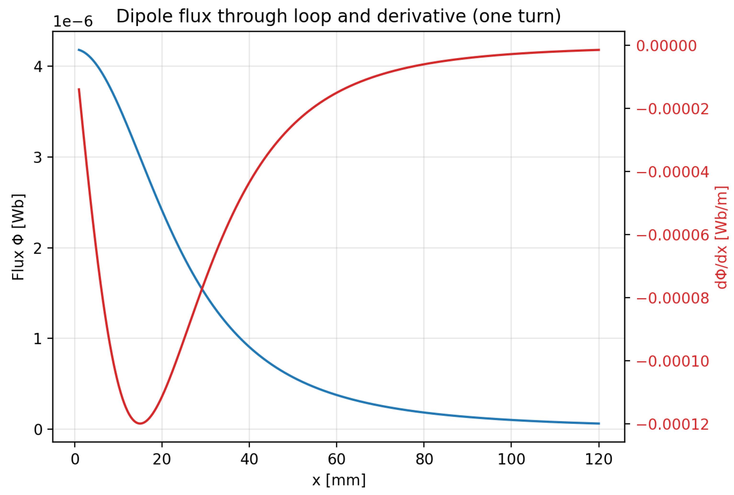
Figure 1. Dipole flux through a circular loop and its derivative: $\mathsf{\Phi }\left(x\right)$ and ${\mathsf{\Phi }}^{\prime }\left(x\right)$ from .

Figure 1. Dipole flux through a circular loop and its derivative: $\mathsf{\Phi }\left(x\right)$ and ${\mathsf{\Phi }}^{\prime }\left(x\right)$ from .

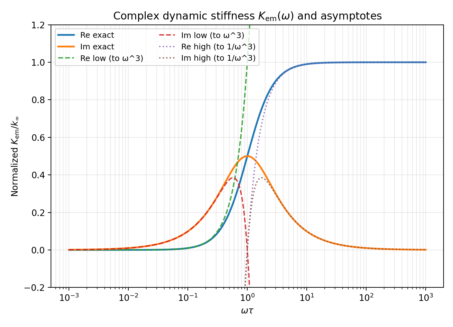
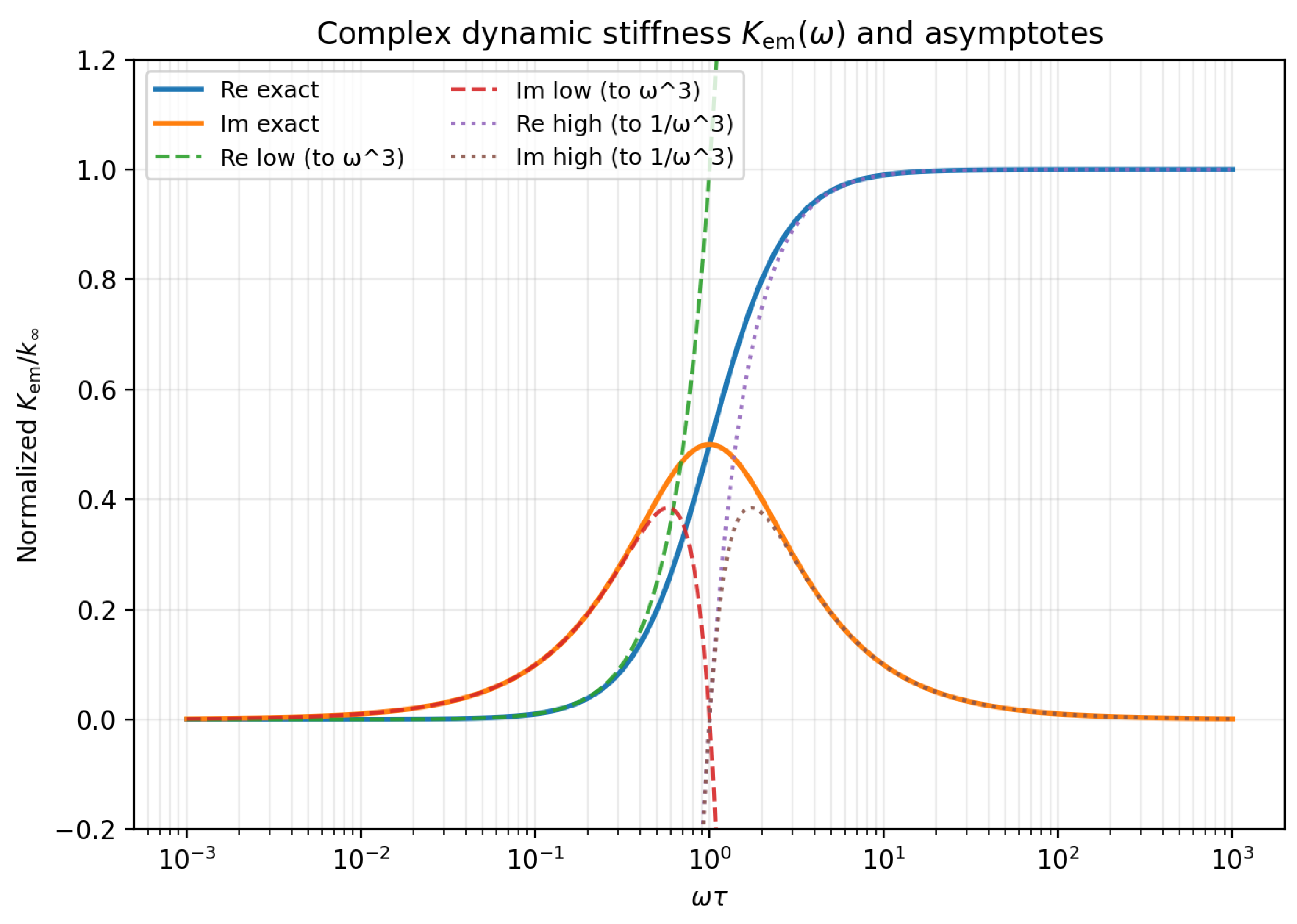
8.3. Complex Dynamic Stiffness and Asymptotes

Figure 2. Normalized complex dynamic stiffness $K_{\mathrm{em}}\left(\omega \right)/k_{\infty }$ vs $\omega \tau$ from Equation (23), with low-frequency (derivative/jerk) and high-frequency (integral/absement-like) asymptotes.

Figure 2. Normalized complex dynamic stiffness $K_{\mathrm{em}}\left(\omega \right)/k_{\infty }$ vs $\omega \tau$ from Equation (23), with low-frequency (derivative/jerk) and high-frequency (integral/absement-like) asymptotes.

8.4. Frequency Scaling of Resistive Loss

Figure 3. Cycle-averaged resistive loss under prescribed harmonic displacement Equation (42), showing $\langle P_R\rangle \propto {\omega }^2$ for $\omega \tau \ll 1$ and a frequency-independent plateau for $\omega \tau \gg 1$.

Figure 3. Cycle-averaged resistive loss under prescribed harmonic displacement Equation (42), showing $\langle P_R\rangle \propto {\omega }^2$ for $\omega \tau \ll 1$ and a frequency-independent plateau for $\omega \tau \gg 1$.

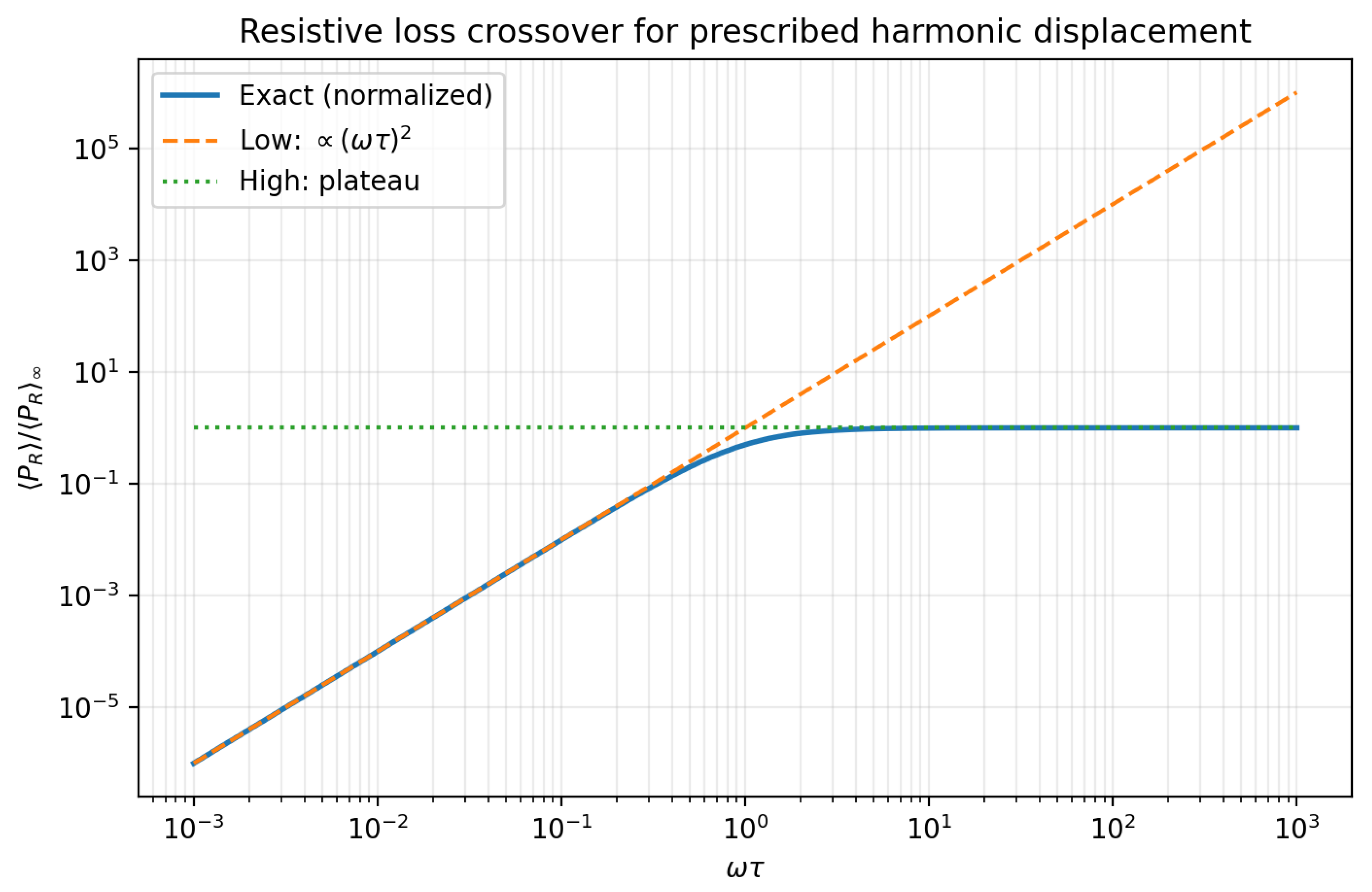
Figure 4. Example ring-down simulation of the coupled nonlinear state–space system 12.

Figure 4. Example ring-down simulation of the coupled nonlinear state–space system 12.

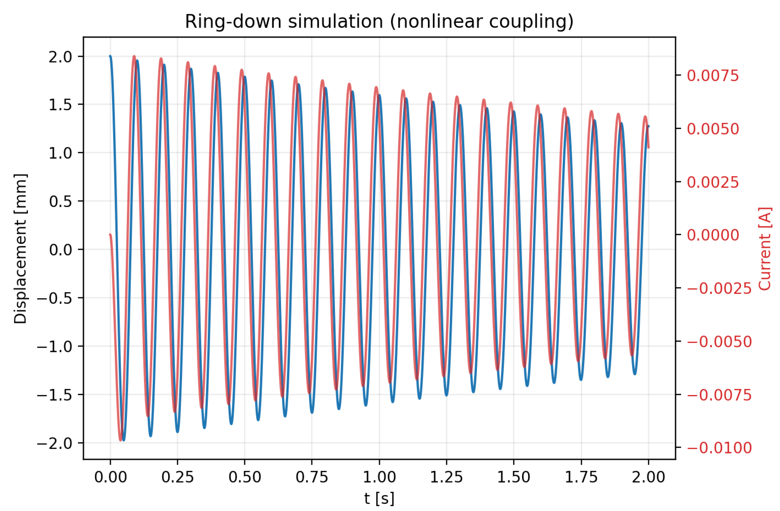
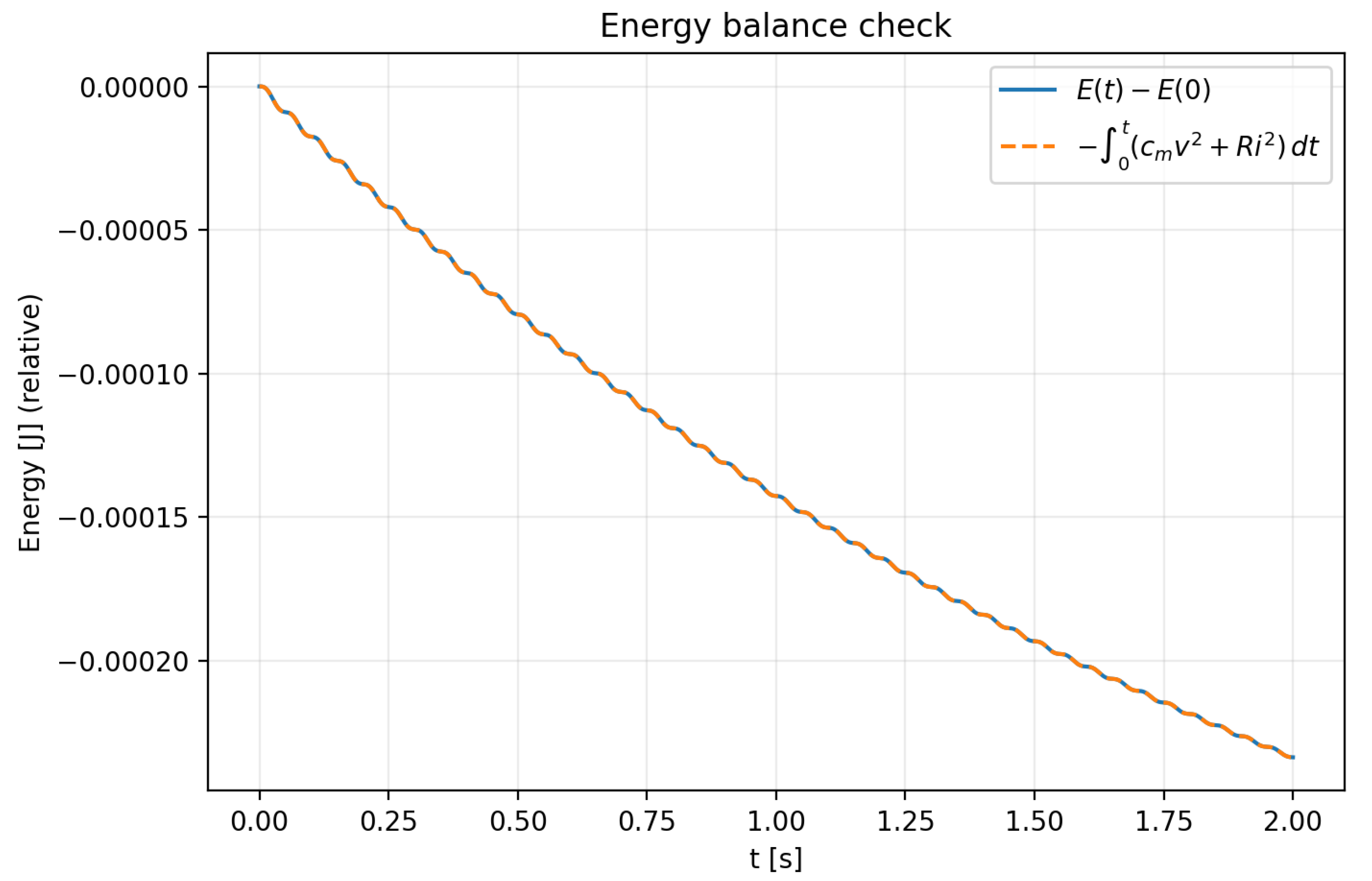
8.5. Time-Domain Ring-Down and Energy Balance

Figure 5. Energy balance check for the ring-down simulation: stored energy $E\left(t\right)$ from Equation (15) compared to cumulative dissipation ${\int }_0^t(c_m{v}^2+R{i}^2)dt$ from Equation (16).

Figure 5. Energy balance check for the ring-down simulation: stored energy $E\left(t\right)$ from Equation (15) compared to cumulative dissipation ${\int }_0^t(c_m{v}^2+R{i}^2)dt$ from Equation (16).

9. Discussion

9.1. Jerk and Absement as Asymptotes of a Passive Kernel

Equations show that jerk-like and absement-like terms arise as controlled asymptotic representations of a single passive electromagnetic memory element. Importantly, these terms are not independent constitutive laws; they are approximations of the exact constitutive behavior and should only be applied within their validity regimes ($\omega \tau \ll 1$ vs $\omega \tau \gg 1$). For general excitations, the internal-state form provides a well-posed and bounded description.

9.2. Connection to Superconducting Systems

The same mathematical structure applies to superconducting loops when R is interpreted as an effective loss mechanism (e.g. flux creep, vortex-motion resistance) and L includes kinetic inductance [8]. In the ideal limit $R\to 0$ (perfect flux conservation), $\tau \to \infty$ and the back-action approaches a purely conservative stiffness $k_{\infty }=G^2/L$ with persistent currents.

9.3. Limitations and Extensions

The dipole approximation neglects finite-size effects and multipole contributions at small separations. The lumped $(R,L)$ description is a minimal model; extended conductors generally exhibit multiple eddy-current modes and therefore a sum of exponentials (distributed relaxation times) rather than a single $\tau$ [3,4]. Nonetheless, the present two-parameter form is a useful reduced-order element and provides a clear route to identification via .

9.3.0.8. Remark (“critical ratio” and a symmetry analogy).

The appearance of the value $t^{★}=x_0/a=1/2$ is a consequence of a balance between the small-t growth $g\left(t\right)\sim t$ and the large-t decay $g\left(t\right)\sim t^{-4}$, yielding a single interior critical point of $g\left(t\right)$. This “central” value $1/2$ is, in a purely formal sense, reminiscent of the role played by $\Re \left(s\right)=1/2$ as the symmetry axis (fixed line) of the involution $s\mapsto 1-s$ in the functional equation of the completed Riemann zeta function. No deeper connection is implied.

10. Conclusions

We derived a minimal, energy-consistent state–space model for a moving magnetic dipole coupled to a conducting (or superconducting) loop. Linearization yields an exact complex dynamic stiffness depending only on $\omega \tau =L\omega /R$ and a stiffness scale $k_{\infty }=G^2/L$. We showed that this electromagnetic back-action is equivalent to a mechanical Maxwell element and provided closed-form expressions for added stiffness, added damping, and direct identification formulas for $(\tau ,k_{\infty })$. The dipole–loop geometry further yields a simple analytic design rule: the coupling gradient (and thus back-action strength) is maximized at $x_0=a/2$. Finally, jerk-like and absement-like force terms were obtained as controlled low- and high-frequency asymptotes of the same passive memory kernel, clarifying their physical meaning and limitations. Reproducible Python simulations validate the theory and provide ready-to-use plots and datasets.

References

- Jackson, J. D. Classical Electrodynamics, 3rd ed.; Wiley, 1998. [Google Scholar]
- Griffiths, D. J. Introduction to Electrodynamics, 4th ed.; Pearson, 2012. [Google Scholar]
- Reitz, J. R. Forces on moving magnets due to eddy currents. Journal of Applied Physics 1970, 41, 2067–2071. [Google Scholar] [CrossRef]
- Saslow, W. M. Maxwell’s theory of eddy currents in a conducting cylinder. American Journal of Physics 1992, 60, 693–711. [Google Scholar] [CrossRef]
- Grover, F. W. Inductance Calculations: Working Formulas and Tables; Dover, 1946. [Google Scholar]
- R. S. Lakes, Viscoelastic Materials; Cambridge University Press, 2009.
- Landau, L. D.; Lifshitz, E. M.; Pitaevskii, L. P. Electrodynamics of Continuous Media, 2nd ed.; Butterworth–Heinemann, 1984. [Google Scholar]
- Tinkham, M. Introduction to Superconductivity, 2nd ed.; McGraw–Hill, 1996. [Google Scholar]
- Smythe, W. R. Static and Dynamic Electricity, 3rd ed.; McGraw–Hill, 1968. [Google Scholar]
- Kraus, J. D.; Fleisch, D. A. Electromagnetics with Applications, 5th ed.; McGraw–Hill, 1999. [Google Scholar]