Submitted:
20 January 2026
Posted:
22 January 2026
You are already at the latest version
Abstract
This study examines the short-run relationship between artificial intelligence (AI), re-newable energy, and economic growth across the G7 countries, China, and South Korea over the 2010–2025 period. Motivated by the ongoing debate on whether AI-driven digital transformation can coexist with environmental sustainability, the analysis integrates technological and energy-economics frameworks. Using panel data and the Fixed Effects (FE) estimator with Driscoll–Kraay robust standard errors, four models (A1–A2–B1–B2) are estimated to explore how AI investment affects economic growth and energy demand. The results reveal that AI investment alone does not significantly enhance short-run economic growth; however, its interaction with renewable energy capacity yields positive and significant effects, confirming the moderating role of sustainable energy infrastructure. Conversely, AI development initially increases energy demand due to the expansion of data-driven infrastructure, but a non-linear (inverted U-shaped) relationship suggests that efficiency improvements emerge beyond a certain adoption threshold. Financial development and energy prices also play significant roles in shaping energy consumption dynamics. Overall, the findings indicate that AI-driven growth and energy efficiency are complementary in the presence of strong renewable capacity and innovation systems. The study provides empirical evidence for integrating AI policies with green energy strategies to foster sustainable digital transformation.
Keywords:
artificial intelligence (AI)
; sustainable economic growth
; renewable energy transition
; energy demand and efficiency
; digital transformation and green innovation
1. Introduction
The rapid integration of Artificial Intelligence (AI) into global production systems is reshaping the foundations of economic growth, technological innovation, and energy consumption. As a general-purpose technology, AI enhances productivity and efficiency across industries, but it also transforms the energy landscape through data centers, computational infrastructure, and automation processes. Understanding how AI investment affects economic growth and interacts with energy systems has therefore become a critical research priority in the era of digital transformation and climate transition.
The interaction between AI-driven technological change and energy systems presents a dual challenge for policymakers. On one hand, AI has the potential to boost productivity and promote sustainable economic growth; on the other hand, the expansion of digital infrastructures in the early stages of adoption can temporarily increase energy demand, offsetting some of these gains. This raises a central policy and research question: Can the economic benefits of AI coexist with environmental sustainability? Addressing this question requires a comprehensive examination of how AI investment, renewable energy capacity, and energy demand jointly influence economic outcomes.
The existing literature provides mixed and sometimes conflicting evidence. Studies such as [1], [2], [3] demonstrate that AI and automation enhance productivity and GDP growth through capital deepening and innovation spillovers. However, [4,5] argue that digitalization may also increase total energy use, generating a rebound effect in which efficiency improvements fail to reduce — and may even raise — aggregate energy consumption. Conversely, [6,7] show that technological learning and renewable energy integration can reverse this pattern over time, enhancing energy efficiency and sustainability. These divergent findings highlight the complexity of the AI–energy–growth nexus and the importance of contextual factors such as renewable energy capacity, R&D intensity, and financial development.
This study contributes to the ongoing debate by empirically examining the short-run effects of AI investments on economic growth and energy demand from a sustainability perspective. Using panel data from the G7 countries, China, and South Korea over the 2010–2025 period, the research tests three core hypotheses
(H1) AI investments have a positive effect on economic growth in the short run;
(H2) the growth-enhancing effect of AI is stronger in countries with higher renewable energy capacity; (moderating effect) and (H3) AI development increases energy demand in the short term but promotes energy efficiency after reaching a certain adoption threshold.
By testing these hypotheses, the study aims to provide new empirical evidence on how digital innovation and the green energy transition jointly shape sustainable growth dynamics.
The main contribution of this research lies in bridging two critical strands of literature — technological economics and energy sustainability — through an integrated empirical framework. The analysis employs the Fixed Effects (FE) estimator with Driscoll–Kraay robust standard errors, which provides consistent results under heteroskedasticity, serial correlation, and cross-sectional dependence. The findings indicate that AI investments alone do not generate immediate growth gains; however, when combined with renewable energy capacity and R&D activities, they contribute to a more sustainable and resilient growth trajectory. Therefore, this study not only enriches the empirical understanding of AI’s macroeconomic role but also provides policy insights for guiding sustainable digital transformation in advanced economies.
2. Theoretical Framework
The theoretical framework of this study has been designed using a multi-layered approach to analyse the macroeconomic effects of artificial intelligence (AI) investments and their symbiotic relationship with energy dynamics. AI investments and the dynamic relationship between sustainable energy and economic growth are primarily addressed within the framework of Neoclassical Growth Theory, Endogenous Growth Theory, and the General Purpose Technologies (GPT) approach. The study positions AI not only as a factor of production but also as a transformative force that alters energy consumption patterns; it synthesises production function-based approaches, complementary asset theories, and environmental economics hypotheses (EKC and Jevons Paradox). The fundamental mechanism, which includes AI investments directly stimulating growth through capital deepening, creating indirect effects through energy demand, and the “moderating” role of the sustainable energy stock in this relationship, is presented in Figure 1. This conceptual framework summarises AI’s need for energy infrastructure as a GPT and the leverage effect of clean energy capacity on growth in a comprehensive flow diagram.
2.1. Neoclassical Approach and Capital Deepening
The potential of artificial intelligence investments to stimulate economic growth is based primarily on the Neoclassical Growth Theory developed by [8,9]. According to this theory, economic growth depends on capital accumulation and labour supply, as well as technological progress, which is considered an external shock. AI investments can be modelled within this framework as a technological shock (Total Factor Productivity - TFP) that increases the efficiency of physical capital and shifts the production possibilities curve outwards. Businesses’ expenditure on AI hardware and software increases output per worker by creating “capital deepening”. This theoretical basis supports the study’s first hypothesis (H1), which posits that AI investments have a positive effect on growth.
2.2. Internal Growth and Knowledge Dissemination
The Endogenous Growth Theory, developed to overcome the limitations of the Solow model which treats technology as exogenous, provides a more comprehensive framework for explaining the long-term effects of AI. According to this approach, proposed by [10,11], technological change is an endogenous result of the economic system and relies on the production of “ideas”. AI, unlike traditional physical capital, is a “non-rivalrous” form of knowledge capital that does not diminish with use. [12] argue that AI is different from traditional capital and is not just a production input but a method that changes innovation itself. AI algorithms and data analytics capabilities provide increasing returns by accelerating R&D processes and facilitating cross-sector knowledge spillovers. In innovation-focused economies such as the G7 countries, AI is not merely a production tool but the fundamental engine that sustains growth as the producer of new innovations.
2.3. General Purpose Technology (GPT) and Energy as a Complementary Asset
The original contribution of this study, the AI and renewable energy interaction (AI X Renewable), is based on the General Purpose Technologies (GPT) theory developed by [13]. Like electricity and the internet, AI is considered a GPT with the potential to transform all sectors [14]. However, the GPT theory emphasises that these technologies require “complementary assets” to increase efficiency. In the context of this study, the energy infrastructure required for AI’s massive data processing capacity is the most critical complementary asset. AI technologies with high energy intensity cannot fully reflect their growth potential when energy supply is limited or costly. Therefore, a sustainable and low-cost energy stock is a factor that leverages AI’s impact on growth. This theoretical mechanism validates the interaction term in the model used in this study and the hypothesis that “AI’s impact is stronger in countries with high sustainable energy capacity” (H2).
2.4. Task-Based Approach and the Jevons Paradox
The dual effect of AI on energy demand and efficiency is explained by the “Task-Based Approach” presented by [15] and the “Jevons Paradox” (Rebound Effect) in environmental economics. According to [15], automation technologies reduce production costs (efficiency effect), leading to economies of scale. However, this increase in productivity can paradoxically increase total resource consumption.
According to this paradox, first proposed by [16] and expanded upon by [17] in modern energy economics, technological progress may reduce energy consumption per unit (efficiency), but total consumption may increase due to lower costs (H3). AI, on the one hand, provides energy efficiency through network optimisation (supply-side efficiency), while on the other hand, it drives up energy demand due to the increasing processing load of data centres (demand-side scale effect). Therefore, in this study, energy demand is modelled not only as an explanatory variable in the growth model but also as a dependent variable affected by AI.
2.5. Temporal Inconsistency in the Relationship Between AI and Energy Demand: The EKC Hypothesis and Scale Effect
The impact of artificial intelligence investments on energy demand follows a non-linear dynamic depending on the time dimension. In this study, the structure of AI, which increases energy consumption in the short term but decreases it (or increases efficiency) in the long term, has been modelled within the framework of the Environmental Kuznets Curve (EKC) hypothesis. The EKC hypothesis, introduced to the literature by [18], predicts an inverted U-shaped relationship between economic growth and environmental degradation (energy consumption). According to this theoretical approach, the technological transformation process occurs in three stages: scale effect, composition effect, and technical effect.
In the short term, the scale effect and energy intensity are at the forefront. The installation and proliferation phase of AI technologies corresponds to the rising part of the EKC (scale effect). Training and operating AI models requires massive data centres and high processing power (GPU/TPU). At this stage, AI is an energy-intensive capital investment. [19] states that AI’s carbon footprint grows exponentially as algorithms become more complex. Therefore, during the early adoption phase of the technology, the “scale effect” prevails due to the expansion of physical infrastructure (data centres, servers), and energy demand increases. This situation theoretically validates this study’s hypothesis that “AI investments increase energy demand in the short term” (H3).
In the long term, the technical impact and efficiency are noteworthy. In the long term, AI’s “technical impact” comes into play. As the level of technological maturity increases, AI algorithms become a tool for optimising energy systems. AI applications such as smart grids, demand-side management, and predictive maintenance minimise losses in energy transmission and distribution. This process corresponds to the decreasing part of the EKC; that is, as technology advances, the energy intensity per unit of output decreases. In their study examining the impact of different types of technology on energy, [20] emphasised that advanced digital technologies take on an energy-saving character in the long term.
A rebound effect may also occur as a threat. The biggest theoretical obstacle to this expected long-term decline is the Rebound Effect (Jevons Paradox). As explained by [17], the energy efficiency provided by AI reduces the effective cost of energy. Lower costs may encourage both producers and consumers to use more digital services. If the “new demand” created by AI (e.g., increased traffic due to the proliferation of autonomous vehicles) outweighs the efficiency gains (less fuel per vehicle), total energy demand may increase rather than decrease. Therefore, the study argues that the net effect of AI on energy depends on the trade-off between technical efficiency gains and increased demand.
2.6. The Leveraging Effect on Growth: Sustainable Energy as a Regulatory Variable
One of the main hypotheses of this study is that the marginal effect of AI investments on economic growth is not constant, but rather varies according to the level of sustainable energy capacity possessed by countries (H2). Statistically positioned as a “moderating variable,” sustainable energy stock is modelled as an external condition that alters the direction or strength of the relationship between the independent variable (AI) and the dependent variable (growth). In the theoretical literature, this mechanism is explained by the Directed Technical Change and Green Growth theories.
Constraining factors must be overcome. The impact of energy-intensive technologies on growth is often hindered by the “resource constraint” barrier in traditional growth models. [21] emphasises that energy inputs are an indispensable complement to capital accumulation and growth. High energy-consuming technologies such as AI, when operating in a fossil fuel-dependent infrastructure, face the risk of “diminishing returns” due to rising energy costs and environmental externalities (carbon taxes, regulations). However, when sustainable energy capacity is high, this resource constraint eases. Clean energy strengthens AI’s contribution to growth (amplification effect) by reducing its operational costs and enabling it to scale without being hampered by environmental regulations.
The synergy between environmental sustainability and efficiency should not be overlooked. According to the Directed Technological Change model developed by [22], technological innovations can be directed towards “dirty” or “clean” technologies. If an economy supports DT investments with clean energy infrastructure, dependence on “dirty” inputs decreases and the returns on innovation increase. In this context, sustainable energy is not just an energy source for DT investments, but a strategic complement that increases its economic efficiency. The interaction term (AI x Renewable) in the model used in this study tests precisely this synergy: as the share of renewable energy increases, the coefficient (elasticity) of AI investment on GDP should increase positively. This situation theoretically confirms that green energy infrastructure acts as a “lever” for AI-based growth.
3. Literature
3.1. The Relationship Between Artificial Intelligence and Growth
[1] have demonstrated the impact of AI and automation on growth at the macro level in the literature. In their study covering 17 countries, including the EU and the US, as well as the G7 countries, and 14 sectors during the period 1993-2007, they found a positive (+) and statistically significant relationship between industrial robot use (the physical proxy for AI) and labour productivity and Total Factor Productivity (TFP). The increase in robot density contributed an average of 0.37 percentage points to annual GDP growth and 0.36 percentage points to labour productivity growth. This effect is close to the impact of the steam engine in the past. The analysis ends in 2007 (it does not cover the modern Deep Learning/Generative AI era). Measuring AI only through “industrial robots” excludes software-based AI (algorithms). [23], who examined US local labour markets (Commuting Zones) for the period 1990-2007, found that automation (robots) positively (+) affected productivity by reducing production costs, but created negative (-) pressure (Displacement Effect) on employment. Adding one robot per thousand workers reduces the employment rate by 0.2 percentage points, while increasing value added and productivity. However, the authors argue that the productivity increase is lower than expected because some technologies are “so-so technology”. This study’s focus solely on US data may not fully reflect the dynamics in other G7 countries (particularly those with high labour protection, such as Germany). [3] is one of the few macro-focused studies that looks directly at the relationship between AI investment and GDP. The study, which covers 60 countries (both developed and developing), also includes time series projections. The findings indicate that AI investments (proxied by ICT and software) have a positive (+) effect on GDP growth, but this effect varies according to countries’ “readiness level” (infrastructure, education). The study predicts that AI’s contribution to global GDP growth could reach 1.2 per cent in the long term. Due to the lack of AI data, the analysis relies heavily on assumptions and proxy variables. It is projection-heavy rather than a definitive analysis of historical data. [24] is important in showing how the impact of AI on labour productivity varies across sectors. The findings of the study, which covered approximately 6,000 companies worldwide (including the US, Europe, and Japan) during the period 2000-2016, identified a positive (+) relationship between AI patent applications and labour productivity. It has been shown that AI innovations increase productivity more than non-AI innovations (Innovation Premium), and that AI patent ownership provides an additional increase (premium) of between 3% and 4% in companies’ labour productivity. The sample, which only included patent-holding firms, may have caused a selection bias towards large/technological firms, and the impact of SMEs was underrepresented. [2] strongly supports the argument that AI is a general-purpose technology. Using industry data from G7 and Eurozone countries for the period 1990-2014, he found that the stock of “Smart Technologies” (AI and Machine Learning) has a positive (+) effect on productivity and that the marginal contribution increases as the technology stock increases (Scale Effect). According to the findings, the productivity elasticity of AI capital is estimated to be between 0.01 and 0.06. In other words, a 10% increase in the AI knowledge stock increased productivity by between 0.1% and 0.6%. Patent data was used as a proxy for AI investments, therefore unpatented (trade secret or open source) AI algorithms were excluded. This may lead to an underestimation of the effect.
These studies empirically demonstrate the positive impact of AI on growth. However, it is thought that more studies are needed that focus on countries such as the G7, which are the home countries of these technologies.
When reviewing the empirical literature summarised in Table 1, it is evident that artificial intelligence (AI) and related automation technologies have a predominantly positive and statistically significant impact on economic growth and productivity. Macro-scale panel data studies such as [1] and [2] reveal that AI supports growth through capital deepening and Total Factor Productivity (TFP), with the magnitude of the effect varying depending on the proxy variable used. In particular, findings by [3] and [24] show that AI investments directly contribute to GDP and labour productivity by creating an “Innovation Premium”. However, [23] deepen the debate on the inclusiveness of growth by pointing out that this increase in productivity may, in some cases, create negative externalities due to the “displacement effect” on employment. While studies in the current literature support the positive effect of AI on growth (H1), they have generally used indirect indicators such as robot stock or patent counts and have mostly concluded their analyses in the mid-2010s.
3.2. The Relationship Between Digitalisation, AI and Energy Demand
While some studies in the literature draw attention to the energy load of data centres ([5]; [4]), others have argued that ICT provides efficiency [6], [7]. [5] present a seminal study representing the “pessimistic” camp, which argues that ICT (and, by extension, AI) may increase overall pollution even if it improves efficiency. This study is not a standard econometric panel data analysis (regression). Instead, it utilised a long-term, large-scale Integrated Assessment Model and scenario simulation linking global systems (economy, energy, population). It was run on a global database covering 183 countries and projected up to 2060. ICT investments and diffusion improve efficiency by reducing energy intensity (energy per GDP) (Technique Effect). However, ICT also strongly stimulates economic growth, thereby increasing total energy demand (Scale Effect). The growth effect created by ICT is greater than the efficiency savings it provides. Therefore, ICT does not reduce total carbon emissions in the long term; rather, it increases them. As the study is a simulation, it presents scenario differences rather than regression coefficients. According to the findings, in the scenario where ICT infrastructure develops rapidly (“High ICT”), carbon emissions are 20% higher than in the baseline scenario. This is a clear example of the Rebound Effect. It is highly sensitive to the assumptions embedded in the IFs model (e.g., the coefficient of how much ICT triggers growth). As it is a study from 2012, it may not fully reflect the radical decline in solar/wind energy costs today and the potential of “Green ICT”. [25], which tests whether ICT trade (technology imports/exports) accelerates the transition to renewable energy and is an important reference for the foreign trade control variable used in this study, found that ICT trade increases energy efficiency and facilitates the transition to renewable energy. However, this effect is not linear; that is, the positive effect strengthens as the scale of technology transfer increases. ICT trade openness positively (+) affects renewable energy consumption.
As this study focuses on developing countries, it reflects the perspective of “consuming” countries rather than “producing” G7 countries. One of the most important critical empirical studies challenging the perception that digitalisation always saves energy and highlighting the Rebound Effect (Jevons Paradox) is that of [4]. The findings reveal that an increase in ICT capital does not reduce energy consumption; on the contrary, it increases it. Although digitalisation improves efficiency, total energy demand increases due to rising economic growth (Scale Effect). A statistically significant positive (+) relationship was found between ICT capital and energy consumption. (This confirms the “short-term increase” part of your H3 hypothesis and the risk of the Jevons Paradox). This study was limited to EU countries. A study by [26] also focuses on AI’s “structural transformative” role, showing how the digital economy changes the energy consumption structure. According to the study’s findings, the digital economy optimises the energy structure by reducing fossil fuel consumption and increasing renewable energy consumption. A 1% increase in the digital economy reduces coal consumption rates (negative coefficient) while increasing clean energy usage rates (positive coefficient). The data set covers a relatively short period. The study by [6] is one of the strongest references proving the asymmetric effects of ICT (Information and Communication Technologies) investments on energy efficiency and carbon emissions in the short and long term, and it supports the short-term and long-term distinction (Model 2) mentioned in this study. According to the findings, a 1% increase in energy efficiency reduces emissions by 1.07% in the short term and 0.37% in the long term. However, it has been observed that ICT investments initially increase energy consumption (positive shock) but balance this in the long term through efficiency. The emission-reducing effect of ICT is significant and negative in the long term (-), but this effect is weaker or positive (consumption-increasing) in the short term.
A critical study examining the impact of the digital economy on the “Green Transition” and supporting its interaction with sustainable energy (H2) has also been proposed by [7]. The findings indicate a non-linear (U-shaped or inverted U-shaped) relationship between the digital economy and energy intensity. Digitalisation begins to reduce energy intensity (efficiency) once it surpasses a certain threshold value. An increase in the digital economy index significantly reduces energy intensity (negative coefficient). However, this effect varies depending on the region’s technological infrastructure (threshold effect). Care should be taken when comparing the results of this study, which focuses on China, with those of the G7 countries. However, the “threshold effect” theory is universal.
As shown in Table 2, the literature presents mixed results regarding the impact of digital technologies on energy demand. Studies such as [4] and [5] argue that total consumption increases due to the scale effect and rebound effect (Positive Direction); studies such as [6] and [7] show that the technique effect becomes dominant as the technology matures and energy intensity decreases in the long term (Negative Direction).
3.3. Energy Consumption, Sustainable Energy and Growth
[27] have demonstrated that there is a two-way causality between renewable energy consumption and economic growth, known as the “Feedback Hypothesis.” That is, energy consumption triggers growth, and growth triggers energy consumption. According to the findings, a 1% increase in renewable energy consumption has a positive effect on GDP. [28] in their study focusing on G7 countries, found that the effect of renewable energy on growth was weaker or statistically insignificant compared to fossil fuels. This indicates that renewable energy technologies were not yet sufficiently widespread or efficient (requiring technological transformation) during the period examined. Furthermore, a clear positive causality could not be identified for every country. [29], in their study of the 38 countries with the highest energy consumption worldwide, found that renewable energy consumption significantly increases economic growth. However, the magnitude of this effect varies according to the level of development of the countries, with the effect being stronger in countries with higher GDP. A 1% increase in renewable energy consumption increases GDP by approximately 0.105%.
[30] concluded that both energy efficiency and renewable energy use support long-term economic growth in EU countries. These findings confirm the positive impact of sustainable energy policies on growth in EU countries. [31], examining the Algerian sample, found a strong positive relationship between energy demand and economic growth. In other words, energy demand positively affects growth. They also found that developments in human capital have a reducing effect on energy demand (improving efficiency). [32], in their study of high-tech institutes in China, found that the effect of technological innovation on energy efficiency is not linear. Innovation has an energy efficiency-enhancing effect once it exceeds a certain threshold value. In other words, although it may be uncertain or negative at the outset, a positive (efficiency-enhancing) effect is observed once the threshold is exceeded.
The literature examining the energy-growth relationship (Table 3) generally supports the ‘Feedback Hypothesis’; that is, energy consumption triggers growth, and growth triggers energy consumption [27]. However, an analysis conducted by [28] specifically for G7 countries shows that the contribution of traditional fossil fuels to growth is still dominant, while renewable energy has not yet created the expected strong impact (for the period in question). In contrast, more recent studies [29], [30] demonstrate that, with technological advances, the coefficient (elasticity) of renewable energy on GDP has increased and become positive. This situation contextualises the assumption (H2) in Model 1 of our study that the AI x Renewable interaction term acts as a catalyst that strengthens the contribution of renewable energy to growth.
4. Materials and Methods
4.1. Data Description and Sources
Table 4 contains the data and sources used. As the question of how artificial intelligence (AI) investments affect economic growth and how this relationship is shaped by sustainable energy capacity is addressed, growth in this context refers not to an increase in total production (GDP) but to an increase in the level of production per capita. In other words, the focus is not on total output but on increases in welfare and productivity. GDP per capita (real, at constant prices) therefore directly captures the impact of AI investments on productivity, the capacity to increase output per capita through capital deepening and technology diffusion. The logarithmic form for GDP per capita approximates the growth rate.
This model appears to be fully consistent with the growth theories of [8] and [10]. Furthermore, almost all empirical studies examining the impact of AI, ICT, or innovation on growth use GDP per capita or GDP per capita growth rate [3], [1], [2].
The Global AI Vibrancy Tool of Stanford University provides AI private investments by country. Total AI Private Investment includes the total amount of private investment (nominal USD) received for AI ventures in a given country. This is because in the models used in this study, the AI Investments variable is defined as “Capital Deepening”. Economically, this means new and active capital entering the production process. According to hypothesis H1 (Economic Growth), “Private Investment” (Venture Capital, PE, etc.) is “fresh money” entering the system for companies to conduct R&D, hire staff, and develop new technologies. This money is directly converted into innovation and production. Therefore, total private investment is the most suitable option for this model. According to hypothesis H3 (Energy Demand), an artificial intelligence venture that receives investment uses a large portion of the money it receives to purchase hardware (GPUs) or lease cloud computing services. In other words, this money is spent directly on energy-consuming infrastructure. The variable that will most strongly test your energy demand hypothesis is the total private investment variable. Since the total AI private investment data is in nominal USD, this data was converted to real USD using the US Consumer Price Index prior to analysis. Otherwise, even if investment appears to have increased, it may actually only be inflation that has risen, and the model may produce misleading results. Other possible investment data included in the Global AI Vibrancy Tool are Total AI Merger/Acquisition (M&A) and Total AI Public Offering (IPO). Total AI Merger/Acquisition (M&A) is when one company acquires another. It is usually a transfer of ownership; that is, no new server is added to the system or new technology is created, only existing technology changes hands. Its impact on energy demand and new capital formation is more indirect than that of “Private Investment”. Total AI Public Offering (IPO) data is highly volatile. One year there may be a massive public offering, the next year there may be none. In panel data analysis (regression), such extreme deviations undermine the validity of your model.
Stanford AI proprietary investment data was used in the short-panel robustness check (Model B) to directly assess AI-specific investment effects. The main analysis was structured to measure long-term effects as well as short-term ones. This approach is consistent with the methodological applications of [1] and [2] which balance data sensitivity and longitudinal depth. In the main analysis (Model A), a longer historical digital capital proxy (ICT-based indicator) was created to ensure long-term consistency and capture the long-term impact of AI investment. The composite index created captures both the physical and digital dimensions of AI investments:
According to this proxy, AI investment is economically based on two fundamental components. These are physical capital (servers, data centres, chips) and knowledge and service capital (software, data science, algorithm exports). The variables used forare the share of ICT goods (such as electronics, computers, telecommunications equipment) in total goods exports (ICT goods exports (% of total goods exports)) and the share of ICT services (such as software, data processing, cloud services, consulting) in total services exports (ICT service exports (% of service exports, BoP)). These variables represent the hardware side and the software and services side of artificial intelligence, respectively. These two variables represent the capital deepening channel of artificial intelligence on economic growth. This method is a variation of the approach favoured in studies such as [1] and [2] while they use “robot stock” or “ICT intensity”, this study measures it from a trade perspective.
The concept of sustainable energy capacity is most accurately represented by the share of installed renewable electricity capacity. The Renewable electricity capacity share (%), which is the ratio of installed renewable energy generation capacity to total installed capacity, both represents infrastructure stock (representing the country’s clean energy potential) and is directly related to the energy-intensive nature of AI investments. As energy supply or consumption data reflect short-term fluctuations, they are inconsistent with the structural-moderator logic of hypothesis H2.
According to the H3 hypothesis, AI investments increase energy demand in the short term and promote energy efficiency in the long term. The hypothesis aims to examine the behaviour of energy demand over time (short-run). Therefore, the energy variable used must reflect both the scale of demand (consumption scale) and efficiency trends (efficiency improvement). Energy use per capita appears appropriate in this regard. This is because, in the short term, AI investment → increased energy use (scale effect), while in the long term, energy use per capita may decrease due to the optimisation effect of AI (efficiency effect). In other words, this variable is the most suitable indicator for measuring the dual nature (scale vs. efficiency) of H3. Therefore, the energy demand dynamics included in the research model (Figure 1) are represented by per capita energy consumption (kg of oil equivalent per capita), consistent with [21], [33], and [32]. This variable reflects both the scale effect of AI-driven economic expansion and the long-term efficiency effect described in H3.
Trade is the sum of exports and imports of goods and services. The trade balance is expressed as a percentage of Gross Domestic Product (GDP), which is the total income generated through the production of goods and services in an economic region during an accounting period.

Table 4.
Variable Descriptions, Data Sources, and Missing Data Completion Methods.
| Variable | Proxy | Source | Time Range | Missing Years1 | Data Completion Procedures |
| Economic Growth | GDP per capita (constant 2015 US$) | World Bank | 2010-2025 | 2025 | Growth Rate Extrapolation (Trend Rate Method) |
| AI Investment (for model B) |
Stanford - Total AI Private Investment2 | The Global AI Vibrancy Tool of Stanford University via [36] | 2017-20243 | - | - |
|
AI Investment (for model A) |
AI Composite Index [(0.5.(ICT Goods Exports (% of total goods exports))+(0.5.(ICT Service Exports (% of service exports, BoP))] |
World Bank |
2010-2024 |
2025 |
Growth Rate Extrapolation (Trend Rate Method) |
| Sustainable Energy Capacity | Renewable electricity capacity share (%) | IRENASTAT Online Data Query Tool via [37] | 2010-2025 | 2025 | Growth Rate Extrapolation (Trend Rate Method) |
| Energy Demand | Energy use per capita (kg oil equivalent per person) | World Bank | 2010-2025 | 2024-2025 | Growth Rate Extrapolation (Trend Rate Method) |
| Trade openness |
Trade (% of GDP) | World Bank | 2010-2025 | 2025 | Growth Rate Extrapolation (Trend Rate Method) |
| Capital Deeping | Gross Fixed Capital Formation (% of GDP) | World Bank | 2010-2025 | 2025 | Growth Rate Extrapolation (Trend Rate Method) |
| CO2 emission | Carbon dioxide (CO2) emissions excluding LULUCF per capita (t CO2e/capita) | World Bank | 2010-2025 | 2025 | Growth Rate Extrapolation (Trend Rate Method) |
| R&D | R&D Expenditure (% of GDP) | World Bank | 2010-2025 | 2024-2025 | Growth Rate Extrapolation (Trend Rate Method) |
| Financial Development | IMF Financial Development Index | International Monetary Fund | 2010-2025 | 2021-2022-2023-2024-2025 | Hibrit Method4 |
| Energy Prices | Energy Price Level PPP Index | World Bank (WDI) | 2010-2025 | 2025 | Growth Rate Extrapolation (Trend Rate Method) |
Note: Growth Rate Extrapolation and Hybrid methods were applied to ensure temporal consistency across 2010–2025 for the G7, China, and South Korea samples.
Gross Fixed Capital Formation (GFCF) — indicates the net increase in productive capacity (machinery, infrastructure, factories, software, etc.) in economies. This is equivalent to the increase in the capital stock (ΔK) in the Neoclassical growth model. In other words, it indicates how much of the income generated in the country is reinvested in productive capital. For this reason, GFCF is directly used as the capital accumulation ratio:
Based on the assumption in this study that “AI investments promote growth through capital deepening,” the validity of the following mechanism is tested in the growth model:
GFCF is a suitable variable for controlling this mechanism econometrically. GFCF has been added to the model because it directly measures physical capital accumulation, is one of the structural determinants of growth alongside AI investments, and is a standard control variable in [8] and [10] type models in the literature.
The main question of this study is based on how AI investments affect economic growth and how this relationship is shaped by sustainable energy capacity and energy demand. In other words, the main question is based on the concept of “sustainable growth”. However, it is known that energy demand or renewable capacity alone is not sufficient to measure sustainability. This is because an economy’s energy consumption may increase, but if this is accompanied by a decrease in carbon intensity, it is a positive outcome in terms of environmental sustainability. Therefore, CO2 emissions are an environmental output of the energy demand channel and an indirect variable that tests the effectiveness of sustainable energy capacity. In other words, Energy demand can increase growth, but if this demand comes from high-carbon-intensity sources, it conflicts with the goal of sustainable growth in the long term. Therefore, the CO2 variable should be included in the model as an output of environmental sustainability.
Models 1 and 2 measure only economic and technological interactions. If CO2 emissions are not included in the model, the environmental quality of energy sources (fossil vs. renewable) is disregarded. This shortcoming has been criticised in the literature. [21] defines the exclusion of the “environmental cost of energy input” in sustainable growth analyses as a methodological weakness, while [38] show that energy-growth analyses that do not include the interaction between renewable energy and CO2 emissions do not reflect the “green growth” context. Therefore, CO2 emissions play the role of a complementary control variable that measures the environmental impact of the energy demand variable. According to [38] per capita land use, land use change and forestry (LULUCF) CO2 emissions (t CO2e/person) were used as a proxy to measure the environmental impact of energy consumption, thus ensuring that only energy-related and industrial sources were considered in the analysis.
In this study, R&D represents technological capacity and innovation level as a control variable. The main effect in the model is already measured by AI Investments. That is, AI investment is used as the source of technology. Therefore, the role of the R&D variable should be to control the overall innovation ecosystem between countries, not AI itself. According to [10], [39], and [38] R&D expenditure (as a percentage of GDP) is used as an indicator of technological capacity and reflects each country’s investment in innovation relative to its economic output. Therefore, R&D, which is the relative economic resources allocated by countries to technology, has been used in the form of R&D Expenditure (% of GDP).
Financial development, which is used to capture elements such as international financial depth, access to credit, and capital market efficiency at the macro level, has been measured using the IMF Financial Development Index, which assesses the depth, accessibility, and efficiency of financial institutions and markets [40], and [41].
The impact of AI investments on energy demand is sensitive to the level of energy prices. (For example, low prices encourage energy use; high prices increase energy efficiency). This effect is at the heart of the “Jevons paradox” debate — that is, even if technological efficiency increases, total demand may rise due to cheap energy. Therefore, energy prices indirectly affect the following two channels:
AI → Energy Demand
Energy Demand → Growth
References such as [21] and [32] have demonstrated that energy prices alter the relationship between technological development and growth through the “cost channel”. Moreover, energy prices reflect both differences in energy intensity between countries and clarify the effect of the sustainable energy capacity variable (because the share of renewable energy is generally inversely related to energy prices). Energy prices have been included in this study as a control variable to capture external shocks that affect both energy demand and economic growth.
4.2. Data Completion Procedures
In line with the studies conducted by [38] and [34], missing annual values were completed using a growth rate extrapolation technique based on the average trend of the previous five years. For smoother variables such as Financial Development, a hybrid approach combining growth rate extrapolation with Kalman-like smoothing (three-year centred moving average) was applied to preserve temporal continuity within the country.
4.2.1. Growth Rate Extrapolation Method
In line with the studies conducted by [38] and [34], missing annual values were completed using a growth rate extrapolation technique based on the average trend of the previous five years. To estimate the missing years in the data using trend growth, the growth rates for the last n years are first calculated:
Projections are then made for the missing years:
or in a repeated manner:
Here, denotes the year for which the last observation is known, g denotes the average annual growth rate (e.g., over the last 5 years), and k denotes the number of years estimated. This method enables short-term extension in the presence of missing data and is frequently used in macroeconomic series [38], and [34].
4.2.2. Hybrid Method (Kalman-Like Smoothing + Growth Rate Extrapolation)
In line with the studies conducted by [35], and [42], a hybrid approach combining Kalman-like correction (three-year centred moving average) with growth rate extrapolation was applied to maintain temporal continuity within the country for smoother variables such as financial development. This method was chosen to complete missing years in the data set and to smooth out volatile financial series while preserving the trend. The methodological steps are as follows.
(a)Smoothing step (Kalman-like, 3-year moving average)
This step reduces short-term fluctuations in the series. A 3-year symmetrical moving average is applied:
Here, the original variable (e.g. Financial Development index), smoothed value, t-1, t and t+1 denote consecutive years. This process can be considered a simplified version of the Kalman filter (trend extraction is performed using deterministic averaging instead of signal extraction).
(b)Growth rate exploration step for missing path
The average growth rate for the last n years of the adjusted series is calculated:
Here, g represents the annual average growth rate. The estimation formula for the missing year t+k is:
Here, is the estimated value, g is the average growth rate over the last five years, and k indicates the number of years projected forward.
(c)Final Hybrid Model
The method can be summarised in two stages:
This formula encompasses both smoothing and lengthening.
4.3. Data Transformations
Following the methodological conventions in panel macro-energy literature [43], [44], and [38], variables expressed in absolute or unbounded scales were log-transformed to enable elasticity interpretation, while bounded ratios and normalized indices were retained in their original form.
GDP per capita shows large cross-country variance and time-based exponential growth trends. The logarithmic transformation reduces heteroskedasticity and allows interpreting coefficients as elasticities of growth. Stanford AI investment data exhibit exponential scaling across years and countries (billions of USD). Logging ensures comparability and converts growth rates into percentage effects. Energy use per capita values are strictly positive and right-skewed. Log transformation aligns with prior literature measuring income–energy elasticity [44], and [45]. Emission data often have heavy right tails. Logarithmic transformation normalises variance and supports log–log specification in environmental Kuznets-type models. The PPP-based energy price index (values > 0) allows log conversion. The coefficient thus represents price elasticity of demand — a standard interpretation in energy economics [27].
ICI (AI Investment Proxy) computed as the mean of ICT goods and services export shares (%). These are ratio indicators (bounded between 0 and 100); taking logs would distort relative proportions. RE (Sustainable Energy Capacity) is a percentage share variable (0/100). Logarithmic conversion not meaningful for percentage-based compositions. Trade (% of GDP) and GFCF (% of GDP) is both are ratio-based macro indicators, not absolute monetary flows. Transforming them would undermine the interpretability of marginal effects. R&D Expenditure (% of GDP) is a ratio variable where the variation is small (typically 0–5%). Logarithm would yield negligible informational gain and may introduce noise. FDI (Financial Development Index) is bounded between 0 and 1. Logarithm not applicable since log (0 < x < 1) produces negative, unbounded values. Instead, the normalised form maintains interpretability as a continuous index.
4.4. Model Framework and Specification
The empirical analysis consists of four models (A1–A2–B1–B2) designed to examine the short-run effects of AI investment on economic growth and energy demand. Models A1 and A2 employ ICT-based proxies for AI investment over 2010–2025, while Models B1 and B2 utilise direct AI private investment data from the Stanford AI Index for 2017–2024. Table 5 shows the analytical framework of the models.
The study is built upon three theoretical hypotheses (H1–H3) that conceptualise the relationships between AI investment, economic growth, and energy demand. To empirically test these hypotheses, four econometric models (A1–A2, B1, and B2) are developed. Each model corresponds to an empirical hypothesis (EH1–EH2) derived from the theoretical framework, as summarised in Table 6.
The initial research design aimed to test both short- and long-run relationships among AI, renewable energy, and economic performance through four hypotheses. However, the absence of cointegration restricted the analysis to short-run estimations. Accordingly, the hypotheses were reformulated to reflect short-term dynamics. This adjustment ensures methodological consistency without altering the study’s theoretical motivation.
Table 7 integrates the theoretical and empirical hypotheses, demonstrating how the conceptual framework (H1–H3) is empirically tested through Models A1–A2 and B1–B2. The table also highlights the inclusion of non-linear terms in the energy demand models to examine potential inverted-U relationships consistent with the Environmental Kuzmet Curve (EKC) Hypothesis.
AI investment contributes to economic growth by enhancing productivity, innovation, and technological efficiency. In the short run, AI investment is expected to have a positive effect on economic growth, although adjustment costs and adoption frictions may delay its measurable impact (H1). Renewable energy moderates the AI–growth relationship by enabling cleaner and more efficient technological diffusion. However, due to the absence of long-term cointegration, this study assesses the balancing role of renewable energy capacity in the short term and focuses on how the intensity of the green transition enhances the growth effects of AI investments (H2). In the short run, AI development increases energy demand, but higher levels of AI adoption are expected to improve efficiency, leading to a nonlinear (inverted U-shaped) relationship consistent with the rebound effect hypothesis (H3)
4.5. Econometric Specification
Based on the structure outlined in Table 5, the econometric formulations of the models are as follows:
Model A1 (Growth Model)
Model A2 (Energy Demand Model)
Model B1 (Growth Model)
Model B2 (Energy Demand Model)
The notation used in the econometric formulations is described as follows:
The subscript i denotes the cross-sectional dimension, representing the individual countries included in the sample (G7, China, and South Korea), while t refers to the time dimension, covering the respective annual observations between 2010 and 2025 (or 2017–2024). The variable indicates the natural logarithm of GDP per capita and serves as the dependent variable in the growth models (Model A1 and Model B1). Similarly, represents the natural logarithm of per capita energy use and is used as the dependent variable in the energy demand models (Model A2 and Model B2). The key explanatory variable denotes the composite proxy of artificial intelligence investment, constructed as the average of ICT goods exports and ICT services exports (both expressed as shares of total exports). In the Model B1 and Model B2, represents the Stanford AI Private Investment Index, which directly measures the annual value of AI-related private investments in each country. refers to the renewable electricity capacity share (%), capturing the contribution of renewable sources to total installed electricity generation capacity. This variable is also interacted with AI-related variables or to assess the moderating role of renewable energy in the AI–growth and AI–energy relationships.
The vector includes a set of macroeconomic and environmental covariates commonly used in the literature, namely: CO2 emissions per capita, R&D expenditure (% of GDP) ), financial development index (IMF composite index) (trade openness (% of GDP), energy price level (PPP-based, ) (and gross fixed capital formation (% of GDP) (). These control variables are incorporated to account for technological progress, institutional quality, and structural differences among countries. The parameters denote country-specific fixed effects that capture unobservable heterogeneity across countries, while represent the stochastic error terms.
Several recent studies e.g., [46]; [34]; [47], [48] highlight that the relationship between technological advancement and energy or environmental outcomes may be non-linear, following an Environmental Kuznets Curve (EKC) pattern. According to this framework, at early stages of technological diffusion, AI-related investments can increase energy consumption due to the scale effect—higher output, data center expansion, and industrial automation all raise energy demand. Beyond a certain threshold, however, efficiency and substitution effects emerge: AI enhances resource optimisation, supports smart grids, and promotes renewable integration, ultimately reducing energy intensity. In order to examine the potential non-linear dynamics between AI development and energy demand, the squared terms of AI investment and are incorporated into Models A2 and B2. This inclusion allows testing whether the relationship follows an inverted-U or U-shaped pattern, consistent with the Environmental Kuznets Curve hypothesis.
A positive sign for and a negative signfor would indicate that AI investment initially increases but later reduces energy demand as technological maturity improves energy efficiency and resource management.
4.6. Estimation Techniques
The empirical estimation employs a Fixed Effects (FE) estimator with Driscoll–Kraay robust standard errors to analyse the short-run relationships between artificial intelligence (AI), renewable energy, economic growth, and energy demand across the G7 countries, China, and South Korea. This approach, developed by [49] and implemented following [50] provides consistent inference under heteroskedasticity, serial correlation, and cross-sectional dependence, conditions frequently encountered in macro-panel datasets involving economically integrated countries. The Fixed Effects (FE) estimator accounts for unobserved country-specific heterogeneity, allowing for the control of time-invariant structural characteristics such as institutional quality, technological capacity, and energy structure. The Driscoll–Kraay covariance matrix corrects the standard errors to ensure robustness against various forms of dependence in the error term, making the estimator particularly suitable for panels with moderate time dimensions (T = 9 and T = 16).
Two groups of models were estimated. In the A1 (AI–Economic Growth) and A2 (AI–Energy Demand) models, which cover the 2010–2025 period (T = 16), the variables lnGDPpc, AIProxy, RE, lnEnergyDemand, and R&D were included in first differences due to their I(1) integration order. All other control variables — Trade, FDI, lnEPL, GFCF, and CO2 emissions — were included in levels, as they were found to be stationary I(0) according to panel unit root and structural break tests. In contrast, the B1 (AI–Economic Growth) and B2 (AI–Energy Demand) models, estimated for the shorter 2017–2025 period (T = 9), include only Trade and RE in first differences, while all remaining variables were incorporated in levels. This adjustment ensures the stationarity of all series and prevents spurious regression bias.
For all models, a lag length of two was specified to capture potential short-memory autocorrelation while preserving degrees of freedom, in line with recommendations by [50]. The estimations were implemented in Stata 17 using the xtscc command, which efficiently computes Driscoll–Kraay standard errors for fixed effects panels with small to moderate time dimensions. This unified estimation strategy provides a consistent and robust framework across the four models (A1–A2–B1–B2), ensuring that inference remains valid despite potential cross-sectional dependence and short panel characteristics. As such, the Driscoll–Kraay FE approach offers reliable short-run evidence on the complex interaction between AI development, renewable energy, and macroeconomic performance in advanced economies.
4.7. Diagnostic and Robustness Tests
Prior to estimation, a series of diagnostic procedures was conducted to ensure the econometric validity of the models. Panel unit root tests, including [51], [52], and [53], [54] were first employed to determine the order of integration for each variable. Given the relatively small time dimension of the dataset (T = 9 for B models and T = 16 for A models), the results from the CIPS test were found to be unstable due to limited degrees of freedom. Therefore, the ADF–PP panel tests were considered more reliable and were used to guide the treatment of variables in first differences or levels.
The Bai–Perron multiple structural break tests [55], and Zivot–Andrews unit root tests [56] were additionally conducted for variables that exhibited non-stationarity at first difference, specifically Trade, lnCO2 and GFCF. The results confirmed the presence of structural shifts consistent with global economic shocks, such as the COVID-19 pandemic, validating the need for robustness corrections in the estimations.
Following the integration and stationarity assessments, all models were estimated using the Fixed Effects estimator with Driscoll–Kraay robust standard errors. This method inherently corrects for heteroskedasticity, autocorrelation, and cross-sectional dependence, as recommended for panels with moderate T and N [49], and [50]. Accordingly, additional diagnostic tests such as the Breusch–Pagan LM, Wooldridge serial correlation, or Pesaran CD tests were not required post-estimation, since their effects were already addressed by the Driscoll–Kraay correction.
The robustness of the results was further verified through comparison across models A1–A2 (T = 16) and B1–B2 (T = 9), where the shorter panels were used to confirm the stability of estimated coefficients. In both datasets, coefficient signs and statistical significance levels were consistent, supporting the reliability of the findings. The use of lag(2) in the Driscoll–Kraay specification also provided an additional safeguard against short-memory autocorrelation while preserving the efficiency of estimates.
Overall, the diagnostic and robustness procedures confirm that the models are statistically sound, well-specified, and free from major econometric concerns. The Fixed Effects estimator with Driscoll–Kraay robust errors provides consistent and reliable inferences regarding the short-run linkages between artificial intelligence, renewable energy, and macroeconomic dynamics across advanced economies.
5. Results
5.1. For Model A1 and A2
Table 8 presents the descriptive statistics of all variables employed in the short-run models (A1 and A2) covering the 2010–2025 period for G7 countries, China, and South Korea. The table reports the number of observations (Obs), mean, standard deviation, minimum, and maximum values for each variable.
The results indicate a balanced panel structure with 144 observations per variable. The mean value of ln(GDP per capita) (10.44) suggests a relatively high income level across the sample, consistent with advanced economies. The average share of renewable electricity capacity (RE = 37.0%) shows a substantial but heterogeneous distribution across countries, reflecting differences in energy transition stages.
The AIProxy variable, constructed as the composite of ICT goods and services exports, exhibits considerable variation (mean = 8.66, SD = 4.95), indicating cross-country differences in AI-related technological activity. Similarly, the interaction term (AIProxy×RE) displays a wide dispersion, implying that the combined influence of AI investment and renewable energy capacity differs significantly among the sample economies.
Among the control variables, the average trade openness is 57.2% of GDP, and gross fixed capital formation averages 24.6%, suggesting robust economic integration and investment activity. CO2 emissions (lnCO2) have moderate dispersion (mean = 2.17), while financial development (FDI index = 0.80) remains high but stable across countries. The average energy price level (lnEPL = 4.53) shows limited variation, reflecting relatively similar energy cost structures within the G7 group.
Overall, the descriptive results highlight a diversified yet comparable macroeconomic and energy profile among advanced and emerging economies, supporting the empirical feasibility of panel-based short-run analysis. Furthermore, the correlation matrix for all variables used in Models A1 and A2 is presented in Table A1 and Table A2 in Appendix A.1.
Table 9 presents the results of cross-sectional dependence (CD) tests for the panel dataset (N = 9, T = 16). The Breusch–Pagan LM test [57] strongly rejects the null hypothesis of cross-sectional independence for Model A1 (p < 0.01), indicating significant interdependence among countries in the short-run growth model. For Model A2, the LM statistic remains significant, while the Pesaran scaled LM and CD tests [58], and [59] fail to reject the null, possibly due to small-N limitations. These results suggest that while economic growth variables exhibit strong common shocks across G7, China, and Korea, energy demand appears more country-specific. Given the evidence of cross-sectional dependence, second-generation panel unit root (CIPS) [60] and cointegration (Westerlund) tests [61], [62] are applied in the next stage to ensure robust inference.
As shown in Table 9, the results of the first-generation tests should be interpreted with caution due to the presence of cross-sectional dependency confirmed in Table 10. Therefore, the results regarding integration orders are based on the CIPS test, which accounts for cross-sectional dependency. The results show that most variables are non-stationary at the level but become stationary after first differencing, indicating integration of order one (I(1)). A few variables, including AIProxy × RE, FDI index, and ln(Energy Price Level PPP), are stationary at level (I(0)), suggesting short-run dynamics consistent with institutional and market-driven factors.
Table 11 presents the structural break test results for the variables that remained non-stationary after first differencing according to the CIPS test, namely Trade, GFCF, and lnCO2. The results from the Zivot–Andrews and Bai–Perron tests confirm the presence of significant structural breaks around 2014–2023, corresponding mainly to the global trade slowdown (2014–2016), the COVID-19 pandemic (2020), and the post-pandemic recovery period (2021–2023). After incorporating these breaks, all three variables exhibit stationarity with structural breaks (I(0) with breaks), supporting the robustness of their inclusion in the panel framework. These results validate that the observed non-stationarity in the CIPS test was likely driven by exogenous shocks rather than stochastic trends, which is consistent with findings in [63] and [64].
For trade, it found 2015 and 2020 in Germany, France, Italy and the United Kingdom; 2019 and 2021 in the USA, the Republic of Korea and Japan; and 2016 and 2020 in Canada and China to be structural break years.
For CO2, 2020 was found to be the structural break year for all countries.
The Zivot-Andrews Test conducted using the Stata programme identified 2023 as the structural break year for GFCF in the USA, the Republic of Korea, Japan, and Italy; 2018 in Germany, France, and China; and 2015 in Canada.
For Trade, it identified 2021 as the structural break year for the USA, Republic of Korea, Japan, Canada, Italy, and the United Kingdom; 2022 for Germany; and 2014 for France.
For CO2, it found 2023 in the USA and Japan; 2020 in Germany and the UK; 2014 in France; 2021 in the Republic of Korea, Canada and China; and 2019 in Italy to be structural break years.
Given the presence of structural breaks and confirmed cross-sectional dependence among panel units (see Table 8), the study proceeds with the [61] error-correction-based panel cointegration test. The Westerlund approach is preferred over traditional residual-based tests (e.g., Pedroni, Kao) because it: Accounts for cross-sectional dependence, incorporates country-specific short-run dynamics, and remains valid in the presence of structural breaks, as documented in [62].
Therefore, applying the Westerlund test at this stage ensures more reliable inference on the long-run equilibrium relationships between AI-related variables, energy demand, and growth, consistent with best practices in recent panel econometric literature.
[61] error-correction-based panel cointegration tests were conducted to examine the existence of a long-run equilibrium relationship between economic growth (lnGDP per capita), artificial intelligence (AI) development, renewable energy capacity, and energy consumption within the A1 model specification. The results across the three versions of the A1 model (A1.1–A1.3) consistently indicate that the null hypothesis of no cointegration cannot be rejected once robust (bootstrap) p-values are considered. Although some conventional p-values (e.g., A1.1 Gt = –3.677, p = 0.004) initially suggest possible long-run linkage, these results lose significance after applying bootstrapped critical values, which are more reliable for panels with small sample dimensions (N=9, T=16). Therefore, after correcting for cross-sectional dependence and finite-sample bias via bootstrapping, no evidence of a stable long-run equilibrium among the variables is found.
Table 12 reports the results of [61] error-correction-based panel cointegration test for different specifications of the A1 model. Bootstrap p-values (1000 replications) are presented to account for cross-sectional dependence. A1 tests include country-specific constants but no deterministic trends. The null hypothesis of no cointegration cannot be rejected at the 5% significance level for any model. Bootstrap critical values were used because cross-sectional dependence among G7, China, and Korea is highly likely due to global energy and technology linkages, asymptotic critical values assume cross-section independence and large T, which are not applicable here, bootstrapping provides finite-sample correction and robust p-values that better approximate the true sampling distribution. This approach is consistent with [65], who emphasize that bootstrapped p-values yield more accurate inference in panels with small N and T.
The division of the A1 model into three submodels was primarily motivated by computational and methodological constraints in Stata 12/17, which limits the xtwest test to a maximum of six covariates. To ensure comprehensive testing of the theoretical framework without overparameterizing the model, control variables were introduced sequentially in sets of two—(A1.1 with Trade and lnCO2), (A1.2 with R&D and FDI), (A1.3 with lnEPL and GFCF).
Table 13 reports the results of [61] error-correction-based panel cointegration test for different specifications of the A2 model. The division of the A2 model into three submodels was primarily motivated by computational and methodological constraints in Stata 12/17, which limits the xtwest test to a maximum of six covariates. To ensure comprehensive testing of the theoretical framework without overparameterizing the model, control variables were introduced sequentially in sets of two—(A2.1 with Trade and lnCO2), (A2.2 with R&D and FDI), (A.2.3 with lnEPL and GFCF).
[61] panel cointegration tests revealed no evidence of a long-run equilibrium relationship among the variables in both Model A1 (AI–Economic Growth nexus) and Model A2 (AI–Energy Demand nexus). Consequently, estimation methods that rely on the presence of cointegration, such as Fully Modified OLS (FMOLS) or Dynamic OLS (DOLS), are not econometrically appropriate in this context.
Given the existence of cross-sectional dependence and the relatively short time dimension (T = 16), the study employed the Fixed Effects estimator with [49] robust standard errors. This estimator corrects for heteroskedasticity, serial correlation, and cross-sectional dependence without requiring cointegration among variables. It allows consistent estimation of short-run effects while controlling for unobserved country-specific heterogeneity. This approach has been widely adopted in small and medium-sized panels where long-run equilibrium cannot be statistically confirmed e.g., [38], [34]. Therefore, the results reflect the short-run dynamic impacts of AI investment, renewable energy capacity, and other controls on economic growth and energy demand rather than long-run equilibrium relationships.
Table 14 reports the Fixed Effects Panel Estimation results with Driscoll–Kraay robust standard errors for Model A1, which explores the relationship between artificial intelligence (AI) development and economic growth across the G7 countries, China, and South Korea for the period 2010–2025. The estimation results indicate that changes in AI activity (ΔAIProxy) do not have a statistically significant direct effect on economic growth in the short run (p = 0.807). This finding suggests that the impact of AI adoption on growth materializes gradually, depending on complementary factors such as digital infrastructure, labor adaptation, and institutional readiness. However, the interaction term between AI and renewable energy capacity (ΔAIProxy × RE) shows a negative and weakly significant coefficient (β = –0.0002, p < 0.10). This implies that while AI and renewable energy individually contribute to modernization, their short-run interaction may initially create adjustment costs—for example, through the high energy requirements of digitalization and renewable infrastructure deployment. This is consistent with the findings of [47], [48], and [34] who emphasize transitional inefficiencies during green digital transformation.
Among the control variables, gross fixed capital formation (GFCF) is positive and statistically significant (β = 0.0041, p < 0.05), confirming that capital accumulation plays a crucial role in stimulating short-run economic growth. Additionally, energy demand (ΔlnEnergyDemand) exerts a strong positive and highly significant effect (β = 0.3994, p < 0.01), indicating that energy consumption remains a key driver of output expansion in advanced economies. This outcome aligns with conventional energy–growth literature emphasizing the energy-growth nexus e.g., [27]. Other variables such as trade openness, CO2 emissions, and R&D expenditure are statistically insignificant, suggesting that their growth-enhancing effects may emerge only in the long term once structural adjustments are complete.
The overall model fit is satisfactory, with a within R2 of 0.5340 and a highly significant F-statistic (F(10,14) = 82.40; p < 0.01). The application of Driscoll–Kraay robust standard errors (maximum lag = 2) ensures reliability against heteroskedasticity, serial correlation, and cross-sectional dependence—issues common in multi-country panels with integrated economies. In summary, the results highlight that while AI investment and renewable capacity individually contribute to modernisation, their joint short-run effects on economic growth are transitional and not yet productivity-enhancing. Over time, as economies adapt to AI-driven technological integration, these effects are expected to become more pronounced and positive.
Table 15 presents the Fixed Effects Panel Estimation results with Driscoll–Kraay robust standard errors for Model A2, which investigates the short-run relationship between artificial intelligence (AI) development and energy demand across G7 countries, China, and South Korea during the 2010–2025 period. The coefficients of both AI activity (ΔAIProxy) and its squared term (ΔAIProxy2) are statistically insignificant, suggesting that AI diffusion has not yet produced measurable effects on energy consumption in the short term. This result reflects the transitional stage of AI integration, where digital infrastructure expansion and data-driven processes may temporarily offset potential efficiency gains. As economies progress toward more advanced AI adoption—particularly in energy management and smart grid systems—these effects are expected to evolve into energy-saving outcomes. Economic growth (ΔlnGDPpc) exhibits a positive and highly significant coefficient (β = 0.7614, p < 0.01), confirming the energy–growth nexus, whereby increased output and income levels are associated with greater energy consumption. Similarly, CO2 emissions per capita (lnCO2) are positively significant (β = 0.0550, p < 0.05), reinforcing the link between energy use and environmental degradation, consistent with previous studies such as [27] and [34]. The Financial Development Index (FDI) displays a positive and statistically significant coefficient (β = 0.1467, p < 0.05), implying that greater financial depth and credit availability promote investment in energy-intensive sectors. This finding aligns with the arguments of [40] and [42], who highlight that financial development stimulates production and investment activities, thus increasing energy demand in the short term. In contrast, the Energy Price Level (lnEPL) variable shows a negative and weakly significant coefficient (β = –0.1504, p < 0.10), suggesting that higher energy prices reduce energy consumption by encouraging efficiency improvements and resource substitution. This supports the theoretical expectation from energy economics that price mechanisms serve as effective short-run tools for moderating energy demand.
Other control variables—such as renewable energy share (ΔRE), trade openness, R&D expenditure, and gross fixed capital formation (GFCF)—are statistically insignificant, implying that their influence on energy demand likely operates through long-term channels rather than immediate effects. The model demonstrates a satisfactory overall fit (within R2 = 0.4717) and a highly significant F-statistic (F(10,15) = 128.58; p < 0.01), confirming the robustness of the model’s explanatory capacity. The use of Driscoll–Kraay robust standard errors (maximum lag = 2) ensures resistance to heteroskedasticity, autocorrelation, and cross-sectional dependence, making the estimates reliable given the moderate time dimension (T = 16). In conclusion, the findings indicate that while AI development has not yet generated short-term reductions in energy demand, economic growth and financial expansion continue to drive energy consumption, whereas higher energy prices exert a moderating effect. These results underline the importance of integrating AI policies with energy pricing and financial sector reforms to guide economies toward energy-efficient digital transformation pathways.
Although Models A1 and A2 were initially specified to capture long-term dynamics, the absence of cointegration among the variables indicates that there is no stable long-term equilibrium relationship between artificial intelligence (AI), renewable energy, and macroeconomic indicators during the sample period. Consequently, these models were estimated in their short-term forms using the Fixed Effects (FE) estimator with Driscoll–Kraay robust standard errors to provide consistent inferences under cross-sectional dependence and autocorrelation.
To further strengthen the empirical robustness of the findings, complementary short-term estimates using Model B1 and B2, with total AI private investment as the primary explanatory variable (an alternative AI measure), are presented in the following section. The fundamental motivation behind this dual model approach is to verify whether the short-term relationships between AI, economic growth, and energy demand are consistent across different proxy representations of AI and to provide further evidence explaining these relationships.
5.2. For Model B1 and B2
Table 16 presents the descriptive statistics for the variables included in the short-run models (B1 and B2), covering the period 2017–2025 for the G7 countries, China, and South Korea. The results indicate sufficient variability across the dataset, supporting the robustness of the short-run econometric estimations. The mean of lnGDP per capita (10.49) suggests relatively high-income economies, while lnAIInvest (20.29) exhibits considerable dispersion, reflecting the heterogeneity in artificial intelligence investment intensity across countries.
The variation in the renewable energy share (RE) and AI × RE interaction term highlights cross-country differences in the degree of integration between technological innovation and clean energy development. The relatively stable distributions of financial development and energy price level (lnEPL) indicate consistent financial and market structures among advanced economies, ensuring comparability of results.
Overall, the descriptive statistics confirm that the panel data possess adequate within- and between-country variation to allow consistent estimation of both the AI–economic growth (Model B1) and AI–energy demand (Model B2) relationships. The balanced structure and moderate dispersion of variables reduce the risk of bias and multicollinearity, thereby enhancing the reliability of subsequent estimations. Furthermore, the correlation matrix for all variables used in Models A1 and A2 is presented in Table A3 and Table A4 in Appendix A.2.
Table 17 presents the results of cross-sectional dependence (CD) tests for Models B1 and B2. The Breusch-Pagan LM, Pesaran Scaled LM, and Pesaran CD tests were conducted to examine the null hypothesis of cross-sectional independence across panel units. For Model B1, all three tests yield statistically significant results at the 1% level (p < 0.01), indicating strong evidence of cross-sectional dependence among countries. This suggests that economic shocks or policy changes in one country are likely to have spillover effects on others. Accordingly, first-generation panel unit root and cointegration tests, which assume independence across cross-sections, would be inappropriate. Instead, the use of second-generation methods such as the CIPS panel unit root test and Westerlund cointegration test is justified.
In contrast, the results for Model B2 are mixed. While the Breusch-Pagan LM test indicates dependence at the 1% level (p = 0.0098), both the Pesaran Scaled LM and CD tests are statistically insignificant (p > 0.8), failing to reject the null of independence. This discrepancy may arise due to the sensitivity of the LM test to panel size (N and T), especially when T is relatively small, as in this dataset. Given these mixed results, cautious interpretation is advised. However, to maintain methodological consistency and comparability, the application of second-generation panel tests remains defensible for Model B2 as well.
Table 18 reports the results of panel unit root tests for the short-run models (B1 and B2). The tests applied include Levin–Lin–Chu (LLC), Im–Pesaran–Shin (IPS), Fisher–ADF, Fisher–PP, and Pesaran’s (2007) CIPS test. However, due to the short time dimension of the panel (T = 9), the CIPS test produced almost identical statistics across all variables, indicating a loss of power and weak discriminatory ability in distinguishing between I(0) and I(1) processes. As noted by [60] and [66], the CIPS test performs reliably only when the time dimension is moderate or large (typically T ≥ 15–20). Hence, in this study, the CIPS results were treated as supplementary rather than decisive.
To ensure reliable identification of the integration order, the panel ADF (Im–Pesaran–Shin) and panel PP (Fisher–PP) tests were primarily used, as these tests exhibit higher power in short panels [52]. Based on these results, most variables were found to be stationary at level (I(0)), while only Trade and Renewable Energy Share of Electricity Capacity (RE) were stationary after first differencing (I(1)). Accordingly, in the short-run estimations (Models B1 and B2), these two variables (Trade and RE) were included in their first-differenced form, while all other variables were used in levels. This approach ensures the robustness and validity of the econometric specification despite the limited time dimension of the dataset.
[61] panel cointegration test could not be applied due to the short time dimension in the sample (T = 9). This test generally requires at least 16 years of time series (T ≥ 16) for error correction dynamics to be estimated in a statistically meaningful way. The limited time dimension in the sample would invalidate the asymptotic properties of the test, thereby reducing the reliability of the results. Therefore, a Fixed Effects (FE) model estimated with robust standard errors by Driscoll–Kraay, which examines short-term relationships, was used.
Table 19 reports the Fixed Effects Panel Estimation results with Driscoll–Kraay robust standard errors for Model B1, which explores the short-run nexus between artificial intelligence (AI) investment and economic growth across the G7 countries, China, and South Korea during the 2017–2025 period. The results show that AI investment (lnAIInvest) has a negative but statistically insignificant coefficient (β = –0.0134, p > 0.10), implying that, in the short run, increases in AI investment may not immediately translate into measurable economic gains. This finding aligns with the literature emphasizing adjustment costs and technology adoption delays in the early phases of digital transformation (Acemoglu & Restrepo, 2020). The interaction term (lnAIInvest × RE) is highly significant and positive (β = 0.0004, p < 0.01), suggesting that the growth effects of AI investment become more pronounced when accompanied by renewable energy expansion. This reflects a synergistic relationship between technological innovation and the green energy transition, where AI facilitates efficiency, optimization, and smart management within renewable energy systems [47], [48]. Although the direct effect of renewable energy share (ΔRE) is positive but statistically insignificant, this outcome reinforces the notion that its independent contribution to short-term growth remains limited, yet its combined effect with AI investments can be substantial through energy efficiency and innovation channels. The gross fixed capital formation (GFCF) variable has a positive and weakly significant coefficient (β = 0.0111, p < 0.10), indicating that capital accumulation continues to support economic expansion, even during periods of technological transformation. Likewise, R&D expenditure is strongly positive and significant (β = 0.0499, p < 0.01), highlighting the critical role of innovation capacity in sustaining digital-age growth. Among the other control variables, trade openness (ΔTrade), CO2 emissions (lnCO2), financial development (FDI), and energy price level (lnEPL) are statistically insignificant, suggesting that their short-run effects are likely muted or operate indirectly through capital accumulation and innovation dynamics. The negative yet insignificant coefficient of lnEPL implies that higher energy prices may exert mild cost pressures on production, temporarily constraining output growth — a finding consistent with short-term adjustment effects in energy-intensive sectors. Overall, the model demonstrates high explanatory power (within R2 = 0.9189) and a strongly significant F-statistic (F(10,15) = 14,482.80; p < 0.01), confirming the robustness of the estimation. The use of Driscoll–Kraay robust standard errors (lag length = 2) ensures consistency in the presence of heteroskedasticity, serial correlation, and cross-sectional dependence — making the results reliable even with a relatively short time dimension (T = 9). In summary, the results indicate that AI investments alone may not yield immediate growth dividends, but when integrated with renewable energy expansion, capital accumulation, and R&D efforts, they foster a sustainable short-run growth trajectory for advanced economies.
Table 20 presents the Fixed Effects Panel Estimation results with Driscoll–Kraay robust standard errors for Model B2, which investigates the short-run relationship between artificial intelligence (AI) development and energy demand across the G7 countries, China, and South Korea for the 2017–2025 period. The estimation results indicate that AIProxy (representing AI activity intensity) has a positive and statistically significant effect on energy demand (β = 0.0898, p < 0.05). This implies that in the short run, an expansion in AI-related activities tends to increase overall energy consumption, likely due to the energy-intensive nature of data centres, machine learning operations, and digital infrastructure. This finding aligns with previous studies e.g., [47], [48], which emphasise that AI technologies initially exert upward pressure on energy demand before potential efficiency gains are realised. Moreover, the squared term of AIProxy (AIProxy2) has a negative and statistically significant coefficient (β = –0.0021, p < 0.05), indicating a nonlinear (inverted U-shaped) relationship between AI and energy demand. This supports the hypothesis that while low to moderate levels of AI adoption increase energy use, beyond a certain threshold, AI-driven optimisation and automation begin to reduce energy intensity. The pattern is consistent with the Environmental Kuznets Curve (EKC) framework extended to digital transformation [46]; [34].
Among the control variables, CO2 emissions (lnCO2) and R&D expenditure (R&D) are strongly positive and statistically significant at the 1% level. This suggests that higher emissions and greater innovation activities coincide with increased energy consumption, likely reflecting the scale effects of industrial activity and technological development in advanced economies. The Financial Development Index (FDI) also has a positive and significant effect (β = 0.3840, p < 0.05), implying that greater financial depth and efficiency are associated with higher energy demand, possibly due to increased access to credit and capital for energy-intensive industries and technological infrastructure. In contrast, Trade openness (ΔTrade) and gross fixed capital formation (GFCF) are negative and statistically significant (p < 0.01), suggesting that economies more integrated into global trade and those investing more efficiently in productive capital tend to improve energy efficiency, leading to lower overall energy demand. The Energy Price Level (lnEPL) variable is weakly negative (p < 0.10), indicating that higher energy prices may slightly discourage consumption and production activities, thereby exerting a moderating effect on short-term energy demand.
The model demonstrates strong overall performance, with a within R2 of 0.9401 and a highly significant F-statistic (F(10,15) = 1567.87; p < 0.01), confirming high explanatory power. The application of Driscoll–Kraay robust standard errors (maximum lag = 2) ensures consistency in the presence of heteroskedasticity, serial correlation, and cross-sectional dependence, which is particularly important for panels with a short time dimension (T = 9). Overall, the findings reveal that AI development initially contributes to higher energy demand but eventually promotes energy efficiency through technological learning and optimisation. This dynamic transition from energy-intensive digital expansion to AI-driven efficiency underscores the dual role of AI in shaping sustainable energy consumption patterns in advanced economies.
6. Discussion
The A1 model examines the short-run interaction between artificial intelligence (AI) investment, renewable energy development, energy demand, and economic growth across G7 countries, China, and South Korea. The findings provide partial support for hypotheses H1, H2, and H3 within a short-run framework. The coefficient of AIProxy, representing AI investment, is positive but statistically insignificant. This indicates that in the short run, AI investments do not generate an immediate and direct impact on economic growth. This finding is consistent with [1], [2], who emphasise that the productivity effects of digital transformation typically emerge over the long term, as they require adaptation, institutional change, and human capital development. Therefore, while H1 is directionally supported, no statistically significant short-run growth effect is detected. In contrast, the interaction term between AI investment and renewable energy capacity (AIProxy × RE) is negative and statistically significant. This result does not support H2 and suggests that the expansion of renewable energy capacity may weaken the short-term growth effect of AI investment. This outcome can be interpreted as a reflection of transitional costs and temporary efficiency losses during the early phases of the green energy shift. Similar findings are reported by [27], [47], [48] who argue that green energy transformation can initially increase production costs and temporarily slow economic growth before long-term benefits materialise. Meanwhile, the variable ΔlnEnergyDemand exerts a positive and strong effect on economic growth, confirming that energy consumption remains a key driver of short-term economic expansion. This result aligns with the traditional growth–energy nexus discussed by [34], [41], [42], and [29] where rising energy demand accompanies higher production and economic activity. In other words, economic expansion and energy consumption reinforce each other in the short run, underscoring the importance of integrating energy security and efficiency policies within broader growth strategies. Among the control variables, R&D expenditure exhibits a negative but statistically insignificant coefficient. This suggests that R&D activity does not yield immediate productivity gains, as innovation effects generally accumulate over time. According to [10] endogenous growth model, the influence of R&D emerges gradually through knowledge accumulation and technological diffusion. Conversely, gross fixed capital formation (GFCF) shows a positive and significant coefficient, indicating that physical capital accumulation continues to play a central role in supporting short-run economic growth. Overall, the results of the A1 model reveal that AI investment has a limited short-term effect on growth, while energy demand exerts a strong positive influence, and the AI–RE interaction temporarily produces a negative effect. These findings suggest that digitalisation and green energy policies may exert opposing effects in the short run but are complementary in the long run. In summary, H1 is directionally supported, H2 is rejected, and H3’s energy efficiency effects are not yet observable in the short run. The evidence indicates that while AI investment alone does not immediately enhance growth, its contribution can strengthen over time when coordinated with energy transition and R&D policies. Policymakers should therefore consider integrating AI, energy security, and renewable energy strategies to achieve sustainable and inclusive economic growth.
The A2 model investigates the short-run impact of artificial intelligence (AI) development on energy demand across the G7 countries, China, and South Korea. The results indicate that both the first difference of AI activity (ΔAIProxy) and its squared term (ΔAIProxy2) are statistically insignificant. This suggests that AI diffusion has not yet generated measurable effects on energy consumption in the short term. As highlighted by [6] and [4] during the early phases of digitalisation, the expansion of energy-intensive digital infrastructure—such as data centres and network systems—may temporarily offset potential efficiency gains. Therefore, the findings imply that AI integration remains in a transitional stage, with its energy-saving potential likely to materialise in the longer term. Economic growth (ΔlnGDPpc) is positive and highly significant, confirming the classical feedback hypothesis between growth and energy consumption: higher output and income levels lead to greater energy demand, while increased energy use supports further production. This finding aligns with [27,34], who demonstrate that growth and energy consumption reinforce each other in advanced economies. Similarly, per capita CO2 emissions (lnCO2) are positive and significant, indicating that higher energy consumption is accompanied by greater environmental pressure. This underscores that in the short run, the growth–energy relationship remains carbon-intensive. The Financial Development Index (FDI) is positive and statistically significant, suggesting that deeper financial systems and increased credit availability promote investment in energy-intensive sectors. This result is consistent with [40,41,42], who emphasise that financial development stimulates production and investment, thereby increasing energy consumption in the short term. In contrast, the Energy Price Level (lnEPL) exhibits a negative and weakly significant coefficient. This finding suggests that higher energy prices reduce energy demand by encouraging efficiency improvements and substitution toward alternative energy sources. It is consistent with theoretical expectations in energy economics, where price mechanisms are viewed as effective short-run tools for moderating energy use. Other control variables—including renewable energy share (ΔRE), trade openness, R&D expenditure, and gross fixed capital formation (GFCF)—are statistically insignificant, implying that their influence on energy demand operates primarily through long-term structural channels. In particular, the share of renewable energy does not yet show a significant short-run impact, as fossil fuels continue to dominate industrial energy consumption during the transition phase. The model demonstrates satisfactory explanatory power (within R2 = 0.4717) and a highly significant F-statistic (F(10,15) = 128.58, p < 0.01), confirming robustness. The use of Driscoll–Kraay robust standard errors ensures that the estimates are consistent under heteroskedasticity, autocorrelation, and cross-sectional dependence, which is especially appropriate for a moderate time dimension (T = 16). Overall, the A2 model findings support the short-run component of H3, indicating that AI development currently exerts an upward effect on energy demand rather than generating efficiency gains. However, this relationship is expected to evolve over time as AI-driven optimisation and smart energy management systems mature. While H1 and H2 are not directly tested in this model, the results highlight that AI’s influence primarily operates through the energy demand channel rather than directly via growth at this stage of technological diffusion. From a policy perspective, these findings emphasise the need to integrate AI strategies with energy pricing, financial system development, and clean energy investment policies. Such coordination would help balance the short-run energy pressures of digital expansion while guiding economies toward a more energy-efficient and sustainable digital transition.
The B1 model examines the short-run relationship between artificial intelligence (AI) investment and economic growth across the G7 countries, China, and South Korea over the 2017–2025 period. The results reveal that AI investment (lnAIInvest) has a negative but statistically insignificant coefficient, indicating that in the short term, the expansion of AI-related investments does not yet yield measurable growth benefits. This finding is consistent with [23], who argue that during the early stages of technological adoption, high adjustment costs, learning inefficiencies, and labour market frictions often delay productivity gains. AI investments typically require complementary capital, digital infrastructure, and human capital adaptation before translating into economic growth, which explains the absence of a significant short-run impact. The interaction term between AI investment and renewable energy share (lnAIInvest × RE) is positive and highly significant, underscoring the synergistic effect between technological innovation and the green energy transition. This suggests that AI investments contribute more effectively to growth when aligned with renewable energy expansion, as AI technologies improve the efficiency, integration, and optimisation of clean energy systems [47], [48]. Such complementarities imply that countries combining digital transformation with energy transition policies experience amplified growth effects—supporting H2, which posits that the growth-enhancing role of AI is stronger in economies with a higher share of sustainable energy capacity. Although the direct coefficient of renewable energy (ΔRE) is positive but insignificant, this outcome highlights that its independent short-run contribution to growth remains modest. Nonetheless, the interaction with AI investment magnifies its overall impact through energy efficiency and technological innovation channels. The positive and weakly significant coefficient of gross fixed capital formation (GFCF) indicates that capital accumulation continues to play a pivotal role in supporting output expansion during digital transformation. This result aligns with the Solow and Romer growth frameworks, where investment in physical and knowledge capital is fundamental for sustaining productivity. R&D expenditure (R&D) shows a strong and statistically significant positive effect on growth, reaffirming the importance of innovation-driven productivity in the digital era. This finding supports H1, which hypothesises that AI-related investments and complementary innovation efforts foster economic growth. Together, these results suggest that AI’s impact is not direct but operates through channels of innovation, renewable energy integration, and capital accumulation, rather than through immediate output increases. Other control variables—including trade openness (ΔTrade), CO2 emissions (lnCO2), financial development (FDI), and energy price level (lnEPL)—are statistically insignificant. This implies that their effects are either indirect or materialize over longer periods. The negative but insignificant coefficient of lnEPL suggests that rising energy prices might impose short-term cost pressures on production, consistent with transition-stage effects in energy-intensive industries. Overall, the B1 model demonstrates high explanatory power (within R2 = 0.9189) and strong statistical significance (F(10,15) = 14,482.80; p < 0.01), confirming the robustness of the results. The use of Driscoll–Kraay robust standard errors (lag length = 2) ensures that the estimates remain consistent under heteroskedasticity, autocorrelation, and cross-sectional dependence—an important consideration given the short time dimension (T = 9). In summary, these findings partially support H1 and H2: while AI investments alone do not produce immediate growth effects, their integration with renewable energy expansion, R&D activity, and capital accumulation fosters a sustainable short-run growth trajectory in advanced economies. However, the results also echo the short-term limitations highlighted in H3, suggesting that the growth dividends of AI are likely to intensify only after the structural and efficiency adjustments of the digital transition are realized
Model B2 examines the short-run relationship between artificial intelligence (AI) development and energy demand across the G7 countries, China, and South Korea during the 2017–2025 period. The results show that the AIProxy variable, representing AI activity intensity, has a positive and statistically significant coefficient (β = 0.0898, p < 0.05). This indicates that in the short term, the expansion of AI-related activities increases overall energy consumption. Such an outcome is primarily due to the energy-intensive nature of data centres, machine learning operations, and digital infrastructure. This finding aligns with [47], [48], who emphasise that AI technologies initially place upward pressure on energy demand before efficiency improvements and optimisation benefits are realized. Furthermore, the squared term of AIProxy (AIProxy2) is negative and statistically significant (β = –0.0021, p < 0.05), suggesting a nonlinear (inverted U-shaped) relationship between AI development and energy demand. This implies that while low to moderate levels of AI adoption raise energy consumption, beyond a certain threshold, AI-driven automation and optimisation begin to reduce energy intensity. This pattern supports the Environmental Kuznets Curve (EKC) hypothesis adapted to digital transformation [46], [34]. Therefore, these findings provide strong evidence in support of H3, which proposes that AI initially increases energy demand in the short run but eventually promotes efficiency and energy-saving outcomes over time. Regarding the control variables, both CO2 emissions (lnCO2) and R&D expenditure (R&D) are positive and highly significant (p < 0.01). This suggests that higher emissions and more intensive innovation activities are associated with greater energy consumption, likely reflecting the scale effects of industrial production and technological activity in advanced economies. The Financial Development Index (FDI) also has a positive and statistically significant effect (β = 0.3840, p < 0.05), indicating that deeper and more efficient financial systems stimulate short-term energy demand by facilitating investment and credit access for energy-intensive industries and technological infrastructure. This result supports the arguments of [40], [41], [42], who highlight that financial development promotes production and investment, thereby raising energy consumption. In contrast, Trade openness (ΔTrade) and gross fixed capital formation (GFCF) are negative and statistically significant (p < 0.01). These findings imply that economies more integrated into global trade and those investing more efficiently in productive capital tend to improve their energy efficiency, resulting in reduced energy demand. Similarly, the Energy Price Level (lnEPL) variable is weakly negative (p < 0.10), suggesting that higher energy prices slightly discourage consumption and production activities, thus exerting a moderating influence on short-run energy demand. The model demonstrates strong overall performance, with a within R2 of 0.9401 and a highly significant F-statistic (F(10,15) = 1567.87; p < 0.01), confirming high explanatory power. The use of Driscoll–Kraay robust standard errors (maximum lag = 2) ensures that the estimates remain consistent under heteroskedasticity, autocorrelation, and cross-sectional dependence — an essential feature for short panels (T = 9). In summary, the results strongly support H3, showing that AI development initially contributes to higher energy demand but eventually fosters efficiency and optimization once technological learning effects materialize. H1 and H2 are partially supported: while economic growth and financial development increase energy consumption, trade openness and capital accumulation contribute to efficiency improvements that mitigate demand. Overall, these findings highlight a dynamic transition from energy-intensive digital expansion to AI-driven energy efficiency, underscoring AI’s dual role in shaping sustainable energy consumption patterns in advanced economies.
Future research could benefit from expanded time-series datasets that encompass a broader historical range of AI-related investment and energy transition data. Such extensions would allow for more comprehensive modelling of long-run causal dynamics, potentially through techniques such as dynamic cointegration frameworks or structural break-adjusted panel estimations. Moreover future research could extend the current framework by investigating country-specific differences in the AI–growth–energy nexus among G7 economies using heterogeneous panel estimators (e.g., Mean Group or PMG models)
Supplementary Materials
The following supporting information can be downloaded at the website of this paper posted on Preprints.org.
Funding
This research received no external funding.
Data Availability Statement
All data sources are listed in the Materials section.
Conflicts of Interest
The authors declare no conflicts of interest.
Abbreviations
The following abbreviations are used in this manuscript:
| G7 | Multidisciplinary Digital Publishing Institute |
| AI | Artificial Intelligence |
| FE | Fixed Effect |
| R&D | Research & Development |
| GPT | General Purpose Technologies |
| EKC | Environmental Kuznets Curve |
| TFP | Total Factor Productivity |
| DT | Direct Technological |
| GDP | Gross Domestic Product |
| EU | European Union |
| US | United States |
| ICT | Information and Communication Technology |
| SMEs | Small and Medium Enterprise |
| OLS | Ordinary Least Square |
| GMM | Generalized Method of Moments |
| OECD | Generalized Method of Moments |
| ARDL | Autoregressive Distributed Lag Model |
| NARDL | Autoregressive Distributed Lag Model |
| VECM | Nonlinear Autoregressive Distributed Lag Model |
| FMOLS | Vector Error Correction Model |
| DOLS | Dynamic Ordinary Least Squares |
| GPUs | Dynamic Ordinary Least Squares |
| M&A | Merger & Acquisition |
| IPO | Total AI Public Offering |
| WDI | World Development Indicators |
| PPP | Purchasing Power Parity |
| GFCF | Gross Fixed Capital Formation |
| IMF | International Monetary Fund |
| FDI | Financial Development Index |
| CIPS | Cross-Sectionally Augmented IPS Test |
| RE | Renewable Energy share of Electricity Capacity |
| EPL | Energy Price Level |
Appendix A
Appendix A.1
Table A1.
Correlation Matrix-Model A1.
| lnGDPpc | AIproxy | RE | AIproxyxRE | lnEnergyDemand | Trade | lnCO2 | R_D | FDI | lnEPL | GFCF | |
| lnGDPpc | 1.0000 | -0.6939 | 0.1044 | -0.5368 | 0.5112 | 0.1345 | 0.1779 | 0.1816 | 0.7663 | 0.4934 | -0.8649 |
| AIproxy | -0.6939 | 1.0000 | -0.2279 | 0.6279 | -0.0733 | -0.0463 | 0.2204 | 0.4001 | -0.4590 | -0.3077 | 0.8797 |
| RE | 0.1044 | -0.2279 | 1.0000 | 0.5479 | -0.0259 | 0.2078 | -0.1430 | -0.4535 | -0.2280 | 0.3994 | -0.1734 |
| AIproxyxRE | -0.5368 | 0.6279 | 0.5479 | 1.0000 | -0.1514 | -0.0639 | 0.0430 | -0.0831 | -0.5403 | -0.0089 | 0.6040 |
| lnEnergyDemand | 0.5112 | -0.0733 | -0.0259 | -0.1514 | 1.0000 | 0.0176 | 0.8357 | 0.2467 | 0.3466 | 0.4960 | -0.1702 |
| Trade | 0.1345 | -0.0463 | 0.2078 | -0.0639 | 0.0176 | 1.0000 | -0.1744 | 0.1268 | -0.1502 | 0.2823 | -0.1539 |
| lnCO2 | 0.1779 | 0.2204 | -0.1430 | 0.0430 | 0.8357 | -0.1744 | 1.0000 | 0.3032 | 0.1516 | 0.5080 | 0.1536 |
| R_D | 0.1816 | 0.4001 | -0.4535 | -0.0831 | 0.2467 | 0.1268 | 0.3032 | 1.0000 | 0.3433 | 0.0887 | 0.1858 |
| FDI | 0.7663 | -0.4590 | -0.2280 | -0.5403 | 0.3466 | -0.1502 | 0.1516 | 0.3433 | 1.0000 | 0.1513 | -0.5735 |
| lnEPL | 0.4934 | -0.3077 | 0.3994 | -0.0089 | 0.4960 | 0.2823 | 0.5080 | 0.0887 | 0.1513 | 1.0000 | -0.3712 |
| GFCF | -0.8649 | 0.8797 | -0.1734 | 0.6040 | -0.1702 | -0.1539 | 0.1536 | 0.1858 | -0.5735 | -0.3712 | 1.0000 |
Table A2.
Correlation Matrix-Model A2.
| lnEnergyDemand | AIproxy | AIProxy2 | lnGDPpc | RE | Trade | lnCO2 | R_D | FDI | lnEPL | GFCF | |
| lnEnergyDemand | 1.0000 | -0.0733 | -0.1299 | 0.5112 | -0.0259 | 0.0176 | 0.8357 | 0.2467 | 0.3466 | 0.4960 | -0.1702 |
| AIproxy | -0.0733 | 1.0000 | 0.9908 | -0.6939 | -0.2279 | -0.0463 | 0.2204 | 0.4001 | -0.4590 | -0.3077 | 0.8797 |
| AIProxy2 | -0.1299 | 0.9908 | 1.0000 | -0.7194 | -0.2016 | -0.0643 | 0.1585 | 0.3477 | -0.4880 | -0.3597 | 0.8759 |
| lnGDPpc | 0.5112 | -0.6939 | -0.7194 | 1.0000 | 0.1044 | 0.1345 | 0.1779 | 0.1816 | 0.7663 | 0.4934 | -0.8649 |
| RE | -0.0259 | -0.2279 | -0.2016 | 0.1044 | 1.0000 | 0.2078 | -0.1430 | -0.4535 | -0.2280 | 0.3994 | -0.1734 |
| Trade | 0.0176 | -0.0463 | -0.0643 | 0.1345 | 0.2078 | 1.0000 | -0.1744 | 0.1268 | -0.1502 | 0.2823 | -0.1539 |
| lnCO2 | 0.8357 | 0.2204 | 0.1585 | 0.1779 | -0.1430 | -0.1744 | 1.0000 | 0.3032 | 0.1516 | 0.5080 | 0.1536 |
| R_D | 0.2467 | 0.4001 | 0.3477 | 0.1816 | -0.4535 | 0.1268 | 0.3032 | 1.0000 | 0.3433 | 0.0887 | 0.1858 |
| FDI | 0.3466 | -0.4590 | -0.4880 | 0.7663 | -0.2280 | -0.1502 | 0.1516 | 0.3433 | 1.0000 | 0.1513 | -0.5735 |
| lnEPL | 0.4960 | -0.3077 | -0.3597 | 0.4934 | 0.3994 | 0.2823 | 0.5080 | 0.0887 | 0.1513 | 1.0000 | -0.3712 |
| GFCF | -0.1702 | 0.8797 | 0.8759 | -0.8649 | -0.1734 | -0.1539 | 0.1536 | 0.1858 | -0.5735 | -0.3712 | 1.0000 |
Appendix A.2
Table A3.
Correlation Matrix-Model B1.
| lnGDPpc | lnAIInvest | RE | AIInvestxRE | lnEnergyDemand | Trade | lnCO2 | R_D | FDI | lnEPL | GFCF | |
| lnGDPpc | 1.0000 | 0.0127 | 0.0290 | 0.0124 | 0.4300 | 0.1997 | 0.1120 | 0.1739 | 0.6823 | 0.5002 | -0.8582 |
| lnAIInvest | 0.0127 | 1.0000 | -0.0519 | 0.1785 | 0.2518 | -0.4825 | 0.3299 | 0.2415 | 0.0869 | -0.0123 | 0.2765 |
| RE | 0.0290 | -0.0519 | 1.0000 | 0.9709 | -0.1091 | 0.2871 | -0.1788 | -0.6423 | -0.3277 | 0.4507 | -0.2785 |
| AIInvestxRE | 0.0124 | 0.1785 | 0.9709 | 1.0000 | -0.0579 | 0.1893 | -0.1048 | -0.5571 | -0.3067 | 0.4418 | -0.1855 |
| lnEnergyDemand | 0.4300 | 0.2518 | -0.1091 | -0.0579 | 1.0000 | -0.0414 | 0.8512 | 0.2512 | 0.2272 | 0.4579 | -0.0516 |
| Trade | 0.1997 | -0.4825 | 0.2871 | 0.1893 | -0.0414 | 1.0000 | -0.2641 | 0.0894 | -0.2399 | 0.3112 | -0.2682 |
| lnCO2 | 0.1120 | 0.3299 | -0.1788 | -0.1048 | 0.8512 | -0.2641 | 1.0000 | 0.3325 | 0.0796 | 0.4520 | 0.2690 |
| R_D | 0.1739 | 0.2415 | -0.6423 | -0.5571 | 0.2512 | 0.0894 | 0.3325 | 1.0000 | 0.3205 | 0.0743 | 0.2154 |
| FDI | 0.6823 | 0.0869 | -0.3277 | -0.3067 | 0.2272 | -0.2399 | 0.0796 | 0.3205 | 1.0000 | 0.1235 | -0.4945 |
| lnEPL | 0.5002 | -0.0123 | 0.4507 | 0.4418 | 0.4579 | 0.3112 | 0.4520 | 0.0743 | 0.1235 | 1.0000 | -0.3766 |
| GFCF | -0.8582 | 0.2765 | -0.2785 | -0.1855 | -0.0516 | -0.2682 | 0.2690 | 0.2154 | -0.4945 | -0.3766 | 1.0000 |
Table A4.
Correlation Matrix-Model B2.
| lnEnergyDemand | lnAIInvest | lnAIInvest2 | lnGDPpc | RE | Trade | lnCO2 | R_D | FDI | lnEPL | GFCF | |
| lnEnergyDemand | 1.0000 | 0.2518 | 0.2533 | 0.4300 | -0.1091 | -0.0414 | 0.8512 | 0.2512 | 0.2272 | 0.4579 | -0.0516 |
| lnAIInvest | 0.2518 | 1.0000 | 0.9969 | 0.0127 | -0.0519 | -0.4825 | 0.3299 | 0.2415 | 0.0869 | -0.0123 | 0.2765 |
| lnAIInvest2 | 0.2533 | 0.9969 | 1.0000 | 0.0159 | -0.0657 | -0.5158 | 0.3369 | 0.2321 | 0.0891 | -0.0323 | 0.2666 |
| lnGDPpc | 0.4300 | 0.0127 | 0.0159 | 1.0000 | 0.0290 | 0.1997 | 0.1120 | 0.1739 | 0.6823 | 0.5002 | -0.8582 |
| RE | -0.1091 | -0.0519 | -0.0657 | 0.0290 | 1.0000 | 0.2871 | -0.1788 | -0.6423 | -0.3277 | 0.4507 | -0.2785 |
| Trade | -0.0414 | -0.4825 | -0.5158 | 0.1997 | 0.2871 | 1.0000 | -0.2641 | 0.0894 | -0.2399 | 0.3112 | -0.2682 |
| lnCO2 | 0.8512 | 0.3299 | 0.3369 | 0.1120 | -0.1788 | -0.2641 | 1.0000 | 0.3325 | 0.0796 | 0.4520 | 0.2690 |
| R_D | 0.2512 | 0.2415 | 0.2321 | 0.1739 | -0.6423 | 0.0894 | 0.3325 | 1.0000 | 0.3205 | 0.0743 | 0.2154 |
| FDI | 0.2272 | 0.0869 | 0.0891 | 0.6823 | -0.3277 | -0.2399 | 0.0796 | 0.3205 | 1.0000 | 0.1235 | -0.4945 |
| lnEPL | 0.4579 | -0.0123 | -0.0323 | 0.5002 | 0.4507 | 0.3112 | 0.4520 | 0.0743 | 0.1235 | 1.0000 | -0.3766 |
| GFCF | -0.0516 | 0.2765 | 0.2666 | -0.8582 | -0.2785 | -0.2682 | 0.2690 | 0.2154 | -0.4945 | -0.3766 | 1.0000 |
| 1 | In line with studies conducted by [34] and [21] growth rate extrapolation (5-year trend) was used for the gaps in recent years, In line with the studies conducted by [35], Kalman Filter-like smoothing (3-year moving average) and Growth Rate Extrapolation (Trend Rate Method) were used together in the data set with 5 years of missing data (International Monetary Fund Financial Development Index) because there was >4 missing data. The purpose of this method is to reduce noise in the series. This method extends the series while preserving the continuity of the trend, suppresses fluctuations, and keeps long-term forecasts realistically stable. Subsequently, the growth extrapolation rate method was used. This approach preserves domestic dynamics and provides a balanced panel estimate. This enables a forward-looking sustainability analysis for the 2025 horizon. |
| 2 | Total AI Private Investment data has been adjusted to real terms using the US Consumer Price Index for all countries. The Consumer Price Index or All Urban Consumers: All Items, US City Average is sourced from the Federal Reserve Bank. Index 1982-1984=100, Seasonally Adjusted. |
| 4 | The Hybrid Method was used because there was >4 missing data points. The Hybrid Method incorporates Kalman Filter-like smoothing (3-year moving average) and Growth Rate Extrapolation (Trend Rate Method) techniques. |
References
- Graetz, G., & Michaels, G. (2018). Robots at work. The Review of Economics and Statistics, 100(5), 753–768. [CrossRef]
- Venturini, F. (2022). Intelligent technologies and productivity spillovers: Evidence from the Fourth Industrial Revolution. Research Policy, 51(10), 104332. [CrossRef]
- Crompton, P., & Kwibuka, D. (2020). Artificial intelligence and economic growth. Journal of Economic Structures, 9, Article 39. [CrossRef]
- Lange, S., Pohl, J., & Santarius, T. (2020). Digitalization and energy consumption. Does ICT reduce energy demand? Ecological Economics, 176, 106760. [CrossRef]
- Moyer, J. D., & Hughes, B. B. (2012). ICTs: Do they contribute to increased carbon emissions? Technological Forecasting and Social Change, 79(5), 919–931. [CrossRef]
- Ramzan, M., Xie, Y., Liu, J., & Fatima, N. (2022). Asymmetric impact of ICT on energy efficiency and carbon emissions: Evidence from OECD countries using Fourier ARDL and NARDL approaches. Energy Economics, 112, 106125. [CrossRef]
- Yi, M., Zhang, Y., Wang, Y., & Sun, P. (2022). Digital economy and energy intensity: Evidence from China. Energy Economics, 107, 105861. [CrossRef]
- Solow, R. M. (1956). A contribution to the theory of economic growth. The Quarterly Journal of Economics, 70(1), 65–94. [CrossRef]
- Swan, T. W. (1956). Economic growth and capital accumulation. Economic Record, 32(2), 334-361. [CrossRef]
- Romer, P. M. (1990). Endogenous technological change. Journal of Political Economy, 98(5, Part 2), S71–S102. [CrossRef]
- Aghion, P., & Howitt, P. (1992). A model of growth through creative destruction. Econometrica, 60(2), 323-351. [CrossRef]
- Cockburn, I. M., Henderson, R. M., & Stern, S. (2018). The impact of artificial intelligence on innovation (NBER Working Paper No. 24449). National Bureau of Economic Research. [CrossRef]
- Bresnahan, T. F., & Trajtenberg, M. (1995). General purpose technologies ‘Engines of growth’?. Journal of Econometrics, 65(1), 83-108. [CrossRef]
- Brynjolfsson, E., Rock, D., & Syverson, C. (2018). Artificial intelligence and the modern productivity paradox: A clash of expectations and statistics. NBER Working Paper Series, No. 24001. National Bureau of Economic Research.
- Acemoglu, D., & Restrepo, P. (2018). The race between man and machine: Implications of technology for growth, factor shares, and employment. American Economic Review, 108(6), 1488-1542. [CrossRef]
- Jevons, W. S. (1865). The Coal Question: An Inquiry Concerning the Progress of the Nation, and the Probable Exhaustion of Our Coal-Mines. Macmillan and Co.
- Sorrell, S. (2009). Jevons’ Paradox revisited: The evidence for backfire from improved energy efficiency. Energy Policy, 37(4), 1456-1469. [CrossRef]
- Grossman, G. M., & Krueger, A. B. (1991). Environmental impacts of a North American free trade agreement. NBER Working Paper Series, No. 3914. National Bureau of Economic Research. [CrossRef]
- Dhar, P. (2020). The carbon impact of artificial intelligence. Nature Machine Intelligence, 2(8), 423-425. [CrossRef]
- Hu, J., Du, H., & Huang, N. (2023). The impact of different types of technology innovation on energy efficiency: Evidence from China’s high-tech industries. Energy, 268, 126662. [CrossRef]
- Bretschger, L. (2009). Energy prices, growth, and the channels in between: Theory and evidence. Resource and Energy Economics, 31(3), 163–179. [CrossRef]
- Acemoglu, D., Aghion, P., Bursztyn, L., & Hemous, D. (2012). The environment and directed technical change. American Economic Review, 102(1), 131-166. [CrossRef]
- Acemoglu, D., & Restrepo, P. (2020). Robots and jobs: Evidence from US labor markets. Journal of Political Economy, 128(6), 2188–2244. [CrossRef]
- Damioli, G., Van Roy, V., & Vertesy, D. (2021). The impact of artificial intelligence on labor productivity. Eurasian Business Review, 11(1), 1–25. [CrossRef]
- Murshed, M. (2020). ICT trade and renewable energy transition: Empirical evidence from South Asian economies. Renewable Energy, 155, 1084–1095. [CrossRef]
- Ren, S., Hao, Y., & Wu, H. (2021). Digitalization and energy structure: Is there a structural transformation effect? Energy Economics, 103, 105616. [CrossRef]
- Apergis, N., & Payne, J. E. (2010). Renewable energy consumption and economic growth: Evidence from a panel of OECD countries. Energy Policy, 38(1), 656–660. [CrossRef]
- Tugcu, C. T., Ozturk, I., & Aslan, A. (2012). Renewable and non-renewable energy consumption and economic growth relationship revisited: Evidence from G7 countries. Energy Economics, 34(6), 1942–1950. [CrossRef]
- Bhattacharya, M., Paramati, S. R., Ozturk, I., & Bhattacharya, S. (2016). The effect of renewable energy consumption on economic growth: Evidence from top 38 countries. Applied Energy, 162, 733–741. [CrossRef]
- Simionescu, M., Strielkowski, W., & Kalyugina, S. (2020). The impact of renewable energy on economic growth: Evidence from Central and Eastern European countries. Energy Reports, 6, 217–223. [CrossRef]
- Bouznit, M., Pablo-Romero, M. P., & Sánchez-Braza, A. (2022a). Economic growth, human capital, and energy consumption in Algeria: Evidence from cointegrating polynomial regression and a simultaneous equations model. Environmental Science and Pollution Research, 30, 23450–23466. [CrossRef]
- Hu, M., Xie, R., & Fang, J. (2023). Renewable energy transition, energy prices, and sustainable economic growth: Evidence from OECD countries. Energy Economics, 120, 106676. [CrossRef]
- Bouznit, M., Pablo-Romero, M. P., & Sánchez-Braza, A. (2022b). Economic growth and energy consumption nexus in MENA countries: A panel data analysis with structural breaks. Energy Economics, 107, 105880. [CrossRef]
- Shahbaz, M., Raghutla, C., Chittedi, K. R., Jiao, Z., & Vo, X. V. (2020). Renewable energy consumption and economic growth nexus: The role of financial development and globalization. Energy Storage, 2(2), e91. [CrossRef]
- Beck, N., & Katz, J. N. (2011). Modeling dynamics in time-series–cross-section political economy data. Annual Review of Political Science, 14(1), 331–352. [CrossRef]
- The Global AI Vibrancy Tool of Stanford University, Stanford - Total AI Private Investment, https://hai.stanford.edu/ai-index/global-vibrancy-tool.
- IRENA (2025), Renewable Energy Statistics 2025, The International Renewable Energy Agency, Abu Dhabi. https://pxweb.irena.org/pxweb/en/IRENASTAT/IRENASTAT__Power%20Capacity%20and%20Generation/RE-SHARE_2025_H2_PX.px?utm_source=chatgpt.com.
- Dogan, E., & Seker, F. (2016). Determinants of CO2 emissions in the European Union: The role of renewable and non-renewable energy. Renewable Energy, 94, 429–439. [CrossRef]
- Ulku, H. (2004). R&D, innovation, and economic growth: An empirical analysis. IMF Working Paper No. 04/185. International Monetary Fund. [CrossRef]
- Levine, R. (2005). Finance and growth: Theory and evidence. In P. Aghion & S. N. Durlauf (Eds.), Handbook of Economic Growth (Vol. 1A, pp. 865–934). Elsevier. [CrossRef]
- Sassi, S., & Goaied, M. (2013b). Financial development, ICT diffusion and economic growth: Lessons from MENA region. Telecommunications Policy, 37(4–5), 252–261. [CrossRef]
- Sassi, S., & Goaied, M. (2013a). Financial development and energy consumption: Evidence from Tunisia. Energy Policy, 61, 1069–1076. [CrossRef]
- Pesaran, M. H., Shin, Y., & Smith, R. J. (1999). Pooled mean group estimation of dynamic heterogeneous panels. Journal of the American Statistical Association, 94(446), 621–634. [CrossRef]
- Stern, D. I. (2004). Economic growth and energy. In C. Cleveland (Ed.), Encyclopedia of Energy (Vol. 2, pp. 35–51). Elsevier. [CrossRef]
- Shaari, M. S., Hussain, N. E., & Ismail, M. S. (2013). Relationship between energy consumption and economic growth: Empirical evidence for Malaysia. Business Systems Review, 2(1), 17–28.
- Dinda, S. (2004). The Environmental Kuznets Curve hypothesis: A survey. Ecological Economics, 49(4), 431–455. [CrossRef]
- Hao, F., Zhang, Y., & Wang, S. (2023). Artificial intelligence, digital transformation, and energy transition: Evidence from global economies. Energy Economics, 124, 106932. [CrossRef]
- Hao, F., Zhang, Y., Song, M., & Zeng, H. (2023). Do digitalization and artificial intelligence reduce energy intensity? Evidence from global panel data. Energy Economics, 122, 106664. [CrossRef]
- Driscoll, J. C., & Kraay, A. C. (1998). Consistent covariance matrix estimation with spatially dependent panel data. Review of Economics and Statistics, 80(4), 549–560.
- Hoechle, D. (2007). Robust standard errors for panel regressions with cross-sectional dependence. Stata Journal, 7(3), 281–312. [CrossRef]
- Levin, A., Lin, C. F., & Chu, C. S. J. (2002). Unit root tests in panel data: Asymptotic and finite-sample properties. Journal of Econometrics, 108(1), 1–24. [CrossRef]
- Im, K. S., Pesaran, M. H., & Shin, Y. (2003). Testing for unit roots in heterogeneous panels. Journal of Econometrics, 115(1), 53–74. [CrossRef]
- Maddala, G. S., & Wu, S. (1999). A comparative study of unit root tests with panel data and a new simple test. Oxford Bulletin of Economics and Statistics, 61(S1), 631–652. [CrossRef]
- Choi, I. (2001). Unit root tests for panel data. Journal of International Money and Finance, 20(2), 249–272. [CrossRef]
- Bai, J., & Perron, P. (2003). Computation and analysis of multiple structural change models. Journal of Applied Econometrics, 18(1), 1–22. [CrossRef]
- Zivot, E., & Andrews, D. W. K. (1992). Further evidence on the great crash, the oil-price shock, and the unit-root hypothesis. Journal of Business & Economic Statistics, 10(3), 251–270. [CrossRef]
- Breusch, T. S., & Pagan, A. R. (1980). The Lagrange Multiplier test and its applications to model specification in econometrics. Review of Economic Studies, 47(1), 239–253. [CrossRef]
- Pesaran, M. H. (2004). General diagnostic tests for cross section dependence in panels. Cambridge Working Papers in Economics, No. 0435, University of Cambridge, Faculty of Economics. [CrossRef]
- Pesaran, M. H., Ullah, A., & Yamagata, T. (2008). A bias-adjusted LM test of error cross-section independence. Econometrics Journal, 11(1), 105–127. [CrossRef]
- Pesaran, M. H. (2007). A simple panel unit root test in the presence of cross-section dependence. Journal of Applied Econometrics, 22(2), 265–312. [CrossRef]
- Westerlund, J. (2007). Testing for error correction in panel data. Oxford Bulletin of Economics and Statistics, 69(6), 709–748. [CrossRef]
- Westerlund, J., & Edgerton, D. L. (2008). A simple test for cointegration in dependent panels with structural breaks. Oxford Bulletin of Economics and Statistics, 70(5), 665–704. [CrossRef]
- Breitung, J., & Das, S. (2005). Panel unit root tests under cross-sectional dependence. Statistica Neerlandica, 59(4), 414–433. [CrossRef]
- Carrion-i-Silvestre, J. L., Kim, D., & Perron, P. (2009). GLS-based unit root tests with multiple structural breaks under both the null and the alternative hypotheses. Econometric Theory, 25(6), 1754–1792. [CrossRef]
- Persyn, D., & Westerlund, J. (2008). Error-correction-based cointegration tests for panel data. The Stata Journal, 8(2), 232–241. [CrossRef]
- Baltagi, B. H. (2021). Econometric analysis of panel data (6th ed.). Springer Nature. [CrossRef]
Figure 1.
Research Model: AI Investments and Sustainable Growth.
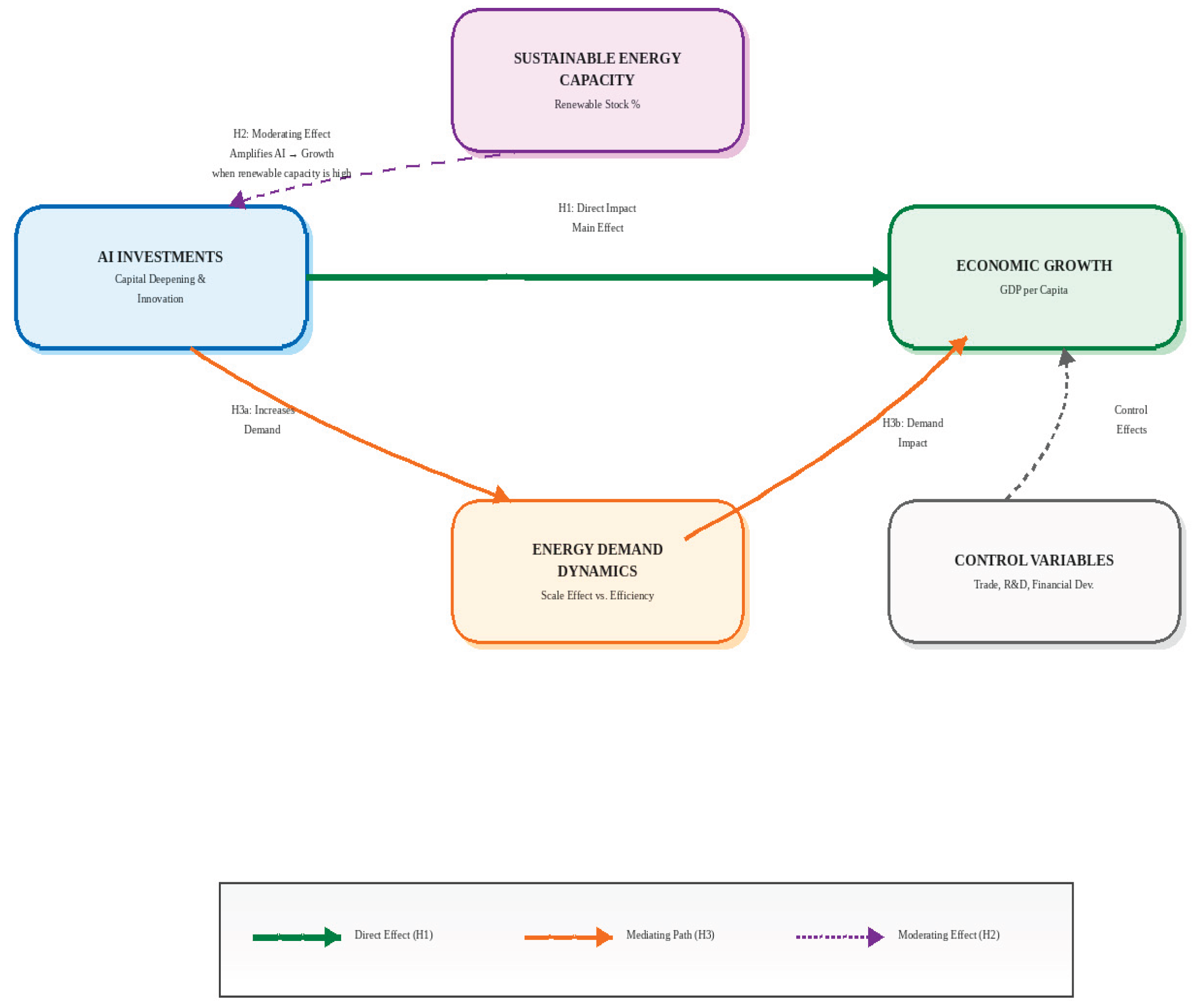
Table 1.
Key Literature on the Relationship between AI and Growth.
| Author(s) | Method | Sample | AI Indicator | Direction of Effect, Coefficient and Key Findings |
| Graetz & Michaels (2018) | OLS/IV | 17 Countries (OECD) | Industrial Robots | (+) %0.36 - %0.37 Contribution: The increase in robot density has contributed 0.37 percentage points to annual GDP growth and 0.36 percentage points to labour productivity. This effect is historically comparable to that of the steam engine. |
| Acemoglu & Restrepo (2020) | OLS Stacked Difference | USA (Local Workforce) | Robot Exposure | (+) Productivity/(-) Employment: Although automation increases productivity, the displacement effect is dominant; each robot reduces the employment rate by 0.2 percentage points. The increase in productivity has been limited due to so-so tech. |
| Damioli et al. (2021) | GMM system | 6,000 Companies (Global) | Patent Family | (+) 3-4% (Innovation Premium): Companies that apply for AI patents achieve an additional 3-4% labour productivity premium compared to those that do not. The effect is more pronounced in the service sector. |
| Venturini (2022) | Dynamic Panel | G7 & EU | Smart Technology Stock | (+) 0.01 - 0.06 (Elasticity): A 10% increase in AI knowledge stock increases efficiency by between 0.1% and 0.6%. It has been proven that AI is a “General Purpose Technology” (GPT) and that the effect strengthens as the stock increases (Scale Effect). |
| Crompton & Kwibuka (2020) | Fixed Effects | 60 Countries | ICT/Software Investment | (+) 1.2% (Long Term): It is projected that AI investments could contribute 1.2% to global growth in the long term. However, the positive impact depends on countries’ infrastructure and education readiness levels. |
Table 2.
Key Literature on the Relationship between Digitalisation, AI and Energy Demand.
| Author(s) | Method | Sample | AI Indicator | Direction of Effect, Coefficient and Key Findings |
| Ramzan et al. (2022) | Fourier ARDL and NARDL | OECD Countries | ICT Investments and Energy Efficiency | Asymmetric Effect: Short-term effect increases emissions (+), long-term effect reduces emissions (-). A 1% increase in efficiency reduces emissions by 0.37% in the long term. |
| Lange et al. (2020) | Panel Data (Fixed Effects) | 19 EU Countries (2000–2017) | ICT Capital Stock | Positive (+)/Rebound Effect: The increase in ICT capital increases total energy consumption rather than saving energy (Jevons Paradox). |
| Yi et al. (2022) | Panel Threshold Model | China (Province Level) | Digital Economy Index | Non-linear (-): There is an inverse U-shaped relationship between the digital economy and energy intensity. Beyond a certain threshold, it reduces energy intensity. |
| Ren et al. (2021) | GMM and Threshold Regression | China (2011–2017) | Digital Economy Development | Structural Transformation (+/-): It reduces fossil fuel consumption (-) while increasing renewable energy consumption (+). |
| Murshed (2020) | Panel ARDL and NARDL | South Asian Economies | ICT Trade Gap | Positive (+): Trade in ICT goods and technology transfer are accelerating the transition to renewable energy. |
| Moyer & Hughes (2012) | International Futures (IFs) Model | Global Projection-183 countries | ICT Development | Positive (+): Although ICT increases efficiency, it is predicted that the growth effect it creates will increase total energy demand in the long term. |
Table 3.
Key Literature on the Relationship between Energy Consumption, Sustainable Energy and Growth.
Table 3.
Key Literature on the Relationship between Energy Consumption, Sustainable Energy and Growth.
| Author(s) | Method | Sample | AI Indicator | Direction of Effect, Coefficient and Key Findings |
| Apergis & Payne (2010) | Panel VECM (Error Correction) | 20 OECD Countries (1985–2005) | Renewable Energy | Two-Way Causality (+): Renewable energy consumption and growth mutually reinforce each other (“Feedback Hypothesis”). A 1% increase in consumption positively impacts GDP. |
| Tugcu et al. (2012) | Panel ARDL (Augmented Production) | G7 Countries (1980–2009) | Renewable vs. Fossil | Neutral or Mixed Results: The impact of renewable energy on growth in G7 countries has been found to be weaker than that of fossil fuels or statistically insignificant (which indicates the need for technological transformation). |
| Bhattacharya et al. (2016) | Panel FMOLS/DOLS | The 38 Countries with the Highest Consumption | Renewable Energy | Positive (+): A 1% increase in renewable energy consumption increases GDP by 0.105%. However, this effect is stronger in countries with high GDP. |
| Simionescu et al. (2020) | Panel ARDL and Bayesian | EU Countries | Renewable & Energy Efficiency | Positive (+): Energy efficiency and renewable energy use support economic growth in the long term. |
| Hu, Du & Huang (2023) | Panel Threshold Model | China (High-Tech Industries) | Energy Efficiency | U-Shaped Relationship: Technological innovation increases energy efficiency once it surpasses a certain threshold. |
| Bouznit et al. (2022a) | Cointegration Polynomial Regression | Algeria | Total Energy | Positive (+): There is a strong positive relationship between energy demand and growth, but human capital has a downward effect on energy demand. |
Table 5.
Variable Definitions and Logarithmic Transformations.
| Variable | Description/Proxy | Symbol | Transformation | Justification |
| Economic Growth | GDP per capita (constant 2015 US$) | lnGDPpc | Logarithmic (ln) | Ensures stationarity and elasticity interpretation |
| AI Investment(for Model B) | Total AI Private Investment (Stanford Index) | lnAIInvest | Logarithmic (ln) | Wide range and exponential scale across countries |
| AI Investment(for Model A) | AI Composite Index [0.5 × (ICT Goods Exports % + ICT Services Exports %)] | AIProxy | Level | Already in ratio form (% of exports); log not meaningful |
| Sustainable Energy Capacity | Renewable electricity capacity share (%) | RE | Level | Percentage ratio (0–100%), logarithmically inapplicable |
| Energy Demand | Energy use per capita (kg oil equivalent per person) | lnEnergyDemand | Logarithmic (ln) | Continuous, positive variable; elasticity interpretation |
| Trade Openness | Trade (% of GDP) | Trade | Level | Ratio variable; bounded within 0–100 |
| Capital Formation | Gross Fixed Capital Formation (% of GDP) | GFCF | Level | Ratio variable, not monetary |
| CO2 Emissions | CO2 emissions per capita (t CO2e/capita) | lnCO2 | Logarithmic (ln) | Continuous, positive, skewed data |
| R&D Expenditure | R&D expenditure (% of GDP) | R&D | Level | Already a ratio; log unnecessary |
| Financial Development | IMF Financial Development Index (0–1 scale) | FDI | Level | Normalised index; log transformation invalid |
| Energy Prices | Energy Price Level (PPP Index, 100 = world avg) | lnEPL | Logarithmic (ln) | Positive index; ln gives elasticity interpretation |
Table 6.
Analytical Framework of the Models.
| Model | Dependent Variable | AI Variable | Period | Empirical Hypothesis Code (EH) and Description | Type |
| A1 | ln(GDP per capita) | AIProxy | 2010–2025 | EH1: AI investment increases short-run growth | Short-run |
| A2 | ln(Energy use per capita) | AIProxy | 2010–2025 | EH2: AI investment reduces short-run energy intensity | Short-run |
| B1 | ln(GDP per capita) | AIInvest | 2017–2024 | EH1: AI investment increases short-run growth | Short-run |
| B2 | ln(Energy use per capita) | AIInvest | 2017–2024 | EH2: AI investment reduces short-run energy intensity | Short-run |
Table 7.
Integration of Theoretical and Empirical Hypotheses Across Model Specifications.
| Theoretical Hypothesis | Theoretical Description | Corresponding Model(s) | Empirical Hypothesis (EH) | Empirical Description | Expected Sign |
| H1 | AI investment positively affects economic growth in the short run. | A1, B1 | AI–growth relationship (EH1) | AI investment (via ICT exports and Stanford AI Index) positively influences economic growth. | + |
| H2 | The growth effect of AI investment is stronger in countries with higher renewable energy capacity. | A1, B1 | Interaction term (AI x RE) |
Renewable energy share strengthens the positive effect of AI on growth (moderating effect). | + |
| H3 |
AI development initially increases energy demand, but higher AI intensity enhances efficiency (rebound hypothesis). |
A2, B2 | AI–energy demand (non-linear) (EH2) | AI investment has a non-linear (inverted-U) impact on energy demand, indicating a potential threshold beyond which AI adoption reduces energy intensity. | +/– |
Table 8.
Descriptive Statistics for Model A1 and A2.
| Variable | Obs | Mean | Std. Dev. | Min | Max |
| lnGDPpc | 144 | 10.43788 | 0.5087724 | 8.659537 | 11.12079 |
| AIProxy | 144 | 8.660539 | 4.948992 | 3.938216 | 22.06608 |
| RE | 144 | 37.02348 | 17.8036 | 3.31 | 71.44731 |
| lnEnergyDemand | 144 | 8.244139 | 0.420266 | 7.549504 | 9.008859 |
| AIProxy x RE | 144 | 300.7002 | 205.5979 | 35.19756 | 1098.519 |
| 144 | 99.32738 | 123.0957 | 15.50955 | 486.9119 | |
| Trade | 144 | 57.20373 | 18.6295 | 23.40156 | 101.6806 |
| GFCF | 144 | 24.57156 | 7.169491 | 16.18113 | 44.07554 |
| lnCO2 | 144 | 2.16736 | 0.4223284 | 1.353915 | 2.88184 |
| R&D | 144 | 2.668515 | 0.9658519 | 1.20155 | 5.84163 |
| FDI | 144 | 0.8050003 | 0.0917837 | 0.511 | 0.9960691 |
| lnEPL | 144 | 4.537153 | .1065964 | 4.356196 | 4.792065 |
Table 9.
Tests for Cross-Sectional Dependence in Panel Data (Model A).
| Model | Test | Test Statistics | P value | Decision | Implications |
| A1 | Breusch-Pagan LM | 126.063*** | 0.0000 | Ho reject | Cross Sectional Dependence exist |
| Pesaran Scaled LM | 5.048*** | 0.0000 | Ho reject | Cross Sectional Dependence exist | |
| Pesaran CD | 5.048*** | 0.0000 | Ho reject | Cross Sectional Dependence exist | |
| A2 | Breusch-Pagan LM | 80.191*** | 0.0000 | Ho reject | Cross Sectional Dependence exist |
| Pesaran Scaled LM | 0.189 | 0.8499 | Ho accept | - | |
| Pesaran CD | 0.189 | 0.8499 | Ho accept | - |
Table 10.
Panel Unit Root Test Results at Level and First Difference (Model A).
| Variable | Levin, Lin & Chu (LLC) | Im, Pesaran & Shin (IPS) |
ADF–Fisher (Maddala-Wu) |
PP–Fisher (Maddala-Wu) |
CIPS (Pesaran) |
Integration Order | |
|
At Level | |||||||
| lnGDPpc | -3.5617*** | -0.7089 | 0.1794 | 2.7302*** | 1.308 | I(1) | |
| AIProxy | -3.7077*** | -0.9016 | 1.8368** | 1.3581* | 0.282 | I(1) | |
| RE | 0.0010 | 1.6912 | -6076 | 3.9689*** | -0.645 | I(1) | |
| lnEnergyDemand | -1.7399** | 0.0884 | 2.6916*** | 4.03547*** | 0.904 | I(1) | |
| AIProxy x RE | -4.7611*** | -1.5712* | 2.5474*** | 1.1419 | -1.561* | I(0) | |
| -3.6260*** | -0.9435 | 1.5542* | 1.4452* | 1.218 | I(1) | ||
| Trade | -4.4887*** | -3.0240*** | 6.4385*** | 1.7469** | 0.778 | I(1) | |
| GFCF | -4.4950*** | -1.2544 | 1.8313** | -1.4145 | -0.134 | I(1) | |
| lnCO2 | -5.2379*** | -2.7502*** | 6.4450*** | 5.0490*** | 0.570 | I(1) | |
| R&D | -2.1063** | 1.0238 | -0.9781 | -0.6486 | -0.619 | I(1) | |
| FDI | -6.0240*** | -3.5713*** | 7.7794*** | 11.9650*** | -5.952*** | I(0) | |
| lnEPL | -3.8186*** | -1.7472** | 2.6627** | 9.9554*** | -1.530* | I(0) | |
|
At First Difference | |||||||
| ΔlnGDPpc | -6.5027*** | -4.6911*** | 8.9534*** | 26.2409*** | -1.842** | I(1) | |
| ΔdAIProxy | -5.3773*** | -3.1907*** | 4.9573*** | 11.7685*** | -3.267*** | I(1) | |
| ΔRE | -7.8542*** | -4.1390*** | 9.0281*** | 4.6528*** | -3.956*** | I(1) | |
| ΔlnEnergyDemand | -7.2805*** | -5.5893*** | 12.7672*** | 30.4791*** | -1.994** | I(1) | |
| ΔAIProxy x RE | -6.7132*** | -4.3857*** | 9.5370*** | 10.5739*** | -4.011*** | I(0) | |
| -5.4736*** | -3.2049*** | 4.9664*** | 12.1844*** | -2.395*** | I(1) | ||
| ΔTrade | -10.0736*** | -6.9646*** | 16.5188*** | 8.4934*** | -1.081 | I(2)Structral break test | |
| ΔGFCF | -4.0751*** | -1.5483* | 1.6736** | 7.9297*** | -.0258 | I(2)Structral break test | |
| ΔlnCO2 | -8.3244*** | -5.6170*** | 12.9348*** | 15.2139*** | -0.195 | I(2)Structral break test | |
| ΔR&D | -4.9805*** | -2.1493** | 2.5657*** | 9.3925*** | -1.639** | I(1) | |
| ΔFDI | -5.6653*** | -5.3726*** | 13.0940*** | 40.6790*** | -4.669*** | I(0) | |
| ΔlnEPL | -8.5482*** | -6.8927*** | 16.7165*** | 41.7421*** | -4.669*** | I(0) | |
Note: The null hypothesis of each test assumes the presence of a unit root. ***, **, * denote significance at the 1%, 5%, and 10% levels, respectively. All tests include both individual intercepts and trends. lag(1) was used for all variables, as it yielded the lowest p-value.
Table 11.
Structural Break and Adjusted Integration Results for Non-Stationary Variables (Trade, GFCF, and lnCO2) (for Model A).
Table 11.
Structural Break and Adjusted Integration Results for Non-Stationary Variables (Trade, GFCF, and lnCO2) (for Model A).
| Variable | CIPS (1st difference) | Zivot Andrews Break | Bai–Perron Breaks | Adjusted Integration Order |
| Trade | Non-stationary | 2014,2020, 2021, 2022 | 2015-2016-2019-2020-2021 | I(0) with breaks |
| GFCF | Non-stationary | 2015,2016, 2018, 2023 | 2014,2015,2016, 2020 | I(0) with breaks |
| lnCO2 | Non-stationary | 2014, 2019, 2020, 2021, 2023 | 2020 | I(0) with breaks |
Note: A separate R code (strucchange) was created for each country and the Bai-Perron Test (strucchange) was performed on the ChatGPT platform for GFCF in Germany, France, Japan, and Canada in 2014 and 2020; Republic of Korea, the United States, Italy, and China in 2015 and 2020; and the United Kingdom in 2016 and 2020 as structural break years.
Table 12.
Westerlund (2007) Panel Cointegration Test Results for the A1 Model (A1.1–A1.3).
| Statistic | Value | Z-value | P-value | Robust P-value | Decision |
| Model A1.1 | |||||
| Gt | -3.677 | -2.625 | 0.004 | 0.578 | No cointegration (bootstrap) |
| Ga | -0.711 | 5.517 | 1.000 | 0.256 | No cointegration |
| Pt | -8.980 | -1.162 | 0.123 | 0.374 | No cointegration |
| Pa | -0.926 | 4.130 | 1.000 | 0.180 | No cointegration |
| Model A1.2 | |||||
| Gt | -2.091 | 2.325 | 0.990 | 0.606 | No cointegration |
| Ga | -0.723 | 5.513 | 1.000 | 0.237 | No cointegration |
| Pt | -3.657 | 3.783 | 1.000 | 0.508 | No cointegration |
| Pa | -0.919 | 4.132 | 1.000 | 0.193 | No cointegration |
| Model A1.3 | |||||
| Gt | -24.064 | -66.268 | 0.000 | 0.477 | No cointegration (bootstrap) |
| Ga | -0.776 | 5.495 | 1.000 | 0.217 | No cointegration |
| Pt | -3.570 | 3.864 | 1.000 | 0.536 | No cointegration |
| Pa | -0.602 | 4.238 | 1.000 | 0.440 | No cointegration |
Note: The lag and lead parameters control the number of dynamic adjustments in the error-correction model. Given the short time dimension (T=16), increasing lag and lead lengths can dramatically reduce degrees of freedom and distort finite-sample properties of the test. Thus, lags(0) and leads(0) were chosen to: Avoid excessive parameterization in a limited time series context, minimize estimation noise, particularly under bootstrap resampling, maintain model stability, consistent with [61] recommendation for panels with T < 20.
Table 13.
Westerlund (2007) Panel Cointegration Test Results for the A2 Model (A2.1–A2.3).
| Statistic | Value | Z-value | P-value | Robust P-value | Decision |
| Model A2.1 | |||||
| Gt | -6.274 | -10.732 | 0.000 | 0.564 | No cointegration (bootstrap) |
| Ga | -0.431 | 5.611 | 1.000 | 0.486 | No cointegration |
| Pt | -9.418 | -1.568 | 0.058 | 0.330 | No cointegration |
| Pa | -0.588 | 4.242 | 1.000 | 0.447 | No cointegration |
| Model A2.2 | |||||
| Gt | -23.078 | -63.188 | 0.000 | 0.542 | No cointegration (bootstrap) |
| Ga | -0.251 | 5.672 | 1.000 | 0.656 | No cointegration |
| Pt | -3.309 | 4.106 | 1.000 | 0.559 | No cointegration |
| Pa | -0.259 | 4.352 | 1.000 | 0.712 | No cointegration |
| Model A2.3 | |||||
| Gt | -2.008 | 2.583 | 0.995 | 0.678 | No cointegration |
| Ga | -0.600 | 5.554 | 1.000 | 0.339 | No cointegration |
| Pt | -3.781 | 3.668 | 1.000 | 0.507 | No cointegration |
| Pa | -1.014 | 4.100 | 1.000 | 0.136 | No cointegration |
Note: The lag and lead parameters control the number of dynamic adjustments in the error-correction model. Given the short time dimension (T=16), increasing lag and lead lengths can dramatically reduce degrees of freedom and distort finite-sample properties of the test. Thus, lags(0) and leads(0) were chosen to: Avoid excessive parameterization in a limited time series context, minimize estimation noise, particularly under bootstrap resampling, maintain model stability, consistent with [61] recommendation for panels with T < 20.
Table 14.
Fixed Effects Panel Estimation with Driscoll–Kraay Robust Standard Errors for Model A1 (AI–Economic Growth Nexus).
Table 14.
Fixed Effects Panel Estimation with Driscoll–Kraay Robust Standard Errors for Model A1 (AI–Economic Growth Nexus).
| Variable | Coef | SE (Drisc-Kraay) | t stat | p-value |
| ΔAIProxy | 0.0008 | 0.0032 | 0.25 | 0.807 |
| ΔRE | 0.0023 | 0.0020 | 1.12 | 0.280 |
| ΔlnEnergyDemand | 0.3994*** | 0.1214 | 3.29 | 0.005 |
| ΔAIProxy x RE | -0.0002* | 0.0001 | -1.81 | 0.092 |
| Trade | 0.0007 | 0.0005 | 1.33 | 0.206 |
| GFCF | 0.0041** | 0.0019 | 2.17 | 0.047 |
| lnCO2 | 0.0172 | 0.0139 | 1.24 | 0.235 |
| ΔR&D | -0.0248 | 0.0378 | -0.66 | 0.522 |
| FDI | -0.0431 | 0.0291 | -1.48 | 0.160 |
| lnEPL | 0.0585 | 0.0639 | 0.92 | 0.375 |
| _cons | 0.3902 | 0.3462 | -1.13 | 0.279 |
| Observations | 135 | |||
| Number of Countries (N) | 9 | |||
| Within | 0.5340 | |||
| F-statistic (10,14) | 82.40 | |||
| Prob>F | 0.0000 | |||
| Maximum lag length | 2 |
Note: The model includes country-specific fixed effects. The estimation is based on annual data for G7 countries, China, and Korea over the 2010–2025 period. The maximum lag length is set to 2. The maximum lag length was automatically set to 2 following the Driscoll–Kraay (1998) and Hoechle (2007) procedure, which determines the optimal bandwidth based on the panel time dimension (T = 16). This ensures heteroskedasticity and autocorrelation consistency of standard errors without over-smoothing in short panels. The first difference of the dependent variable (ΔlnGDPpc) has been included. ***,**,* state that p < 0.01, p < 0.05, p < 0.1 significance levels, respectively.
Table 15.
Fixed Effects Panel Estimation with Driscoll–Kraay Robust Standard Errors for Model A2 (AI-Energy Demand Nexus).
Table 15.
Fixed Effects Panel Estimation with Driscoll–Kraay Robust Standard Errors for Model A2 (AI-Energy Demand Nexus).
| Variable | Coef | SE (Drisc-Kraay) | t stat | p-value |
| ΔAIProxy | -0.0026 | 0.0083 | -0.32 | 0.751 |
| 0.00003 | 0.0002 | 0.13 | 0.898 | |
| ΔlnGDPpc | 0.7614*** | 0.1171 | 6.50 | 0.000 |
| ΔRE | -0.0022 | 0.0022 | -1.00 | 0.333 |
| Trade | -0.0007 | 0.0009 | -0.81 | 0.429 |
| GFCF | -0.0003 | 0.0024 | -0.14 | 0.891 |
| lnCO2 | 0.0550** | 0.0210 | 2.62 | 0.020 |
| ΔR&D | -0.0372 | 0.0340 | -1.10 | 0.292 |
| FDI | 0.1467** | 0.0529 | 2.77 | 0.015 |
| lnEPL | -0.1504* | 0.0821 | -1.83 | 0.089 |
| _cons | 0.4809 | 0.4550 | 1.06 | 0.308 |
| Observations | 135 | |||
| Number of Countries (N) | 9 | |||
| Within | 0.4717 | |||
| F-statistic (10,15) | 128.58 | |||
| Prob>F | 0.0000 | |||
| Maximum lag length | 2 |
Note: The model includes country-specific fixed effects. The estimation is based on annual data for G7 countries, China, and Korea over the 2010–2025 period. The maximum lag length is set to 2. The maximum lag length was automatically set to 2 following the [49], [50] procedure, which determines the optimal bandwidth based on the panel time dimension (T = 16). This ensures heteroskedasticity and autocorrelation consistency of standard errors without over-smoothing in short panels. The first difference of the dependent variable (ΔlnEnergyDemand) has been included. ***,**,* state that p < 0.01, p < 0.05, p < 0.1 significance levels, respectively.
Table 16.
Descriptive Statistics for Model B1 and B2.
| Variable | Obs | Mean | Std. Dev. | Min | Max | |
| lnGDPpc | 81 | 10.493 | 0.4555464 | 9.129295 | 11.12079 | |
| lnAIInvest | 81 | 20.29848 | 1.948427 | 14.07895 | 24.48767 | |
| RE | 81 | 42.97693 | 15.89222 | 9.11 | 71.44731 | |
| lnEnergyDemand | 81 | 8.21518 | 0.4252944 | 7.579608 | 9.008859 | |
| AIInvest x RE | 81 | 870.7795 | 326.8756 | 163.1027 | 1499.28 | |
| 81 | 415.7779 | 78.59134 | 198.2168 | 599.6462 | ||
| Trade | 81 | 57.55373 | 18.51778 | 23.40156 | 90.58515 | |
| GFCF | 81 | 24.95475 | 6.742851 | 17.57946 | 42.38038 | |
| lnCO2 | 81 | 2.108521 | 0.4376658 | 1.353915 | 2.804807 | |
| R&D | 81 | 2.866025 | 1.052828 | 1.37013 | 5.84163 | |
| FDI | 81 | 0.8204327 | 0.0842391 | 0.627 | 0.9960691 | |
| lnEPL | 81 | 4.533998 | 0.1082658 | 4.368054 | 4.761832 |
Table 17.
Tests for Cross-Sectional Dependence in Panel Data (Model B).
| Model | Test | Test Statistics | P value | Decision | Implications |
| B1 | Breusch-Pagan LM | 67.417*** | 0.0041 | Ho reject | Cross Sectional Dependence exist |
| Pesaran Scaled LM | 3.045*** | 0.0023 | Ho reject | Cross Sectional Dependence exist | |
| Pesaran CD | 3.045*** | 0.0023 | Ho reject | Cross Sectional Dependence exist | |
| B2 | Breusch-Pagan LM | 58.690*** | 0.0098 | Ho reject | Cross Sectional Dependence exist |
| Pesaran Scaled LM | -0.222 | 0.8243 | Ho accept | - | |
| Pesaran CD | -0.222 | 0.8243 | Ho accept | - |
Table 18.
Panel Unit Root Test Results at Level and First Difference (Model B).
| Variable | Levin, Lin & Chu (LLC) | Im, Pesaran & Shin (IPS) |
ADF–Fisher (Maddala-Wu) |
PP–Fisher (Maddala-Wu) |
CIPS (Pesaran) |
Integration Order | ||
|
At Level |
||||||||
| lnGDPpc | -6.1524*** | -0.7123 | 1.8336** | 7.0639*** | 1.700 | I(0) | ||
| lnAIInvest | -3.7077*** | -0.0797 | 0.4976 | 4.8101*** | 1.700 | I(0) | ||
| RE | -4.0270*** | 1.4189 | 0.2958 | -2.1138 | 1.700 | I(1) | ||
| lnEnergyDemand | -6.1016*** | -0.6203 | 0.9055 | 7.8384*** | 1.700 | I(0) | ||
| lnAIInvest x RE | -4.2088*** | 0.2398 | -0.2243 | 4.5123*** | 1.700 | I(0) | ||
| -4.8947*** | -0.1680 | 0.5585 | 4.3883*** | 1.700 | I(0) | |||
| Trade | -10.4420*** | -2.3804*** | 4.0723*** | -1.3325 | 1.700 | I(1) | ||
| GFCF | -3.6794*** | 0.9315 | -1.3208 | 4.8929*** | 1.700 | I(0) | ||
| lnCO2 | -9.1412*** | -2.2757** | 5.4211*** | 8.3863*** | 1.700 | I(0) | ||
| R&D | -28.5214*** | -1.1397 | 5.1247*** | 7.5134*** | 1.700 | I(0) | ||
| FDI | -83.1339*** | -19.8437*** | 27.9536*** | 13.2954*** | 1.700 | I(0) | ||
| lnEPL | -9.6366*** | -1.7985** | 7.8732*** | 1.6669** | 1.700 | I(0) | ||
|
At First Difference |
||||||||
| ΔlnGDPpc | -9.0240*** | -1.1032 | 3.1851*** | 9.9710*** | 1.700 | I(0) | ||
| ΔlnAIInvest | -10.4784*** | -1.7168** | 5.0362*** | 6.3014*** | 1.700 | I(0) | ||
| ΔRE | -12.7635*** | -2.6596*** | 9.5938*** | 13.5139*** | 1.700 | I(1) | ||
| ΔlnEnergyDemand | -18.5970*** | -6.0242*** | 19.6333*** | 25.4430*** | 1.700 | I(0) | ||
| ΔlnAIInvest x RE | -6.9317*** | -0.7395 | 1.4038* | 17.4570*** | 1.700 | I(0) | ||
| -10.1641*** | -1.5847* | 4.5023*** | 5.8000*** | 1.700 | I(0) | |||
| ΔTrade | -8.9508*** | -0.7893 | 0.4808 | 8.4934*** | 1.700 | I(1) | ||
| ΔGFCF | -6.1203*** | 0.0439 | -0.3003 | 5.0083*** | 1.700 | I(0) | ||
| ΔlnCO2 | -16.6586*** | -4.6664*** | 16.3110*** | 16.0866*** | 1.700 | I(0) | ||
| ΔR&D | -10.1213*** | -0.8307 | 4.5374*** | 14.7916*** | 1.700 | I(0) | ||
| ΔFDI | -5.6653*** | -5.3726*** | 13.0940*** | 40.6790*** | 1.700 | I(0) | ||
| ΔdlnEPL | -7.6882*** | -1.3950* | 4.5919*** | 10.5217*** | 1.700 | I(0) | ||
Note: The null hypothesis of each test assumes the presence of a unit root. ***, **, * denote significance at the 1%, 5%, and 10% levels, respectively. All tests include both individual intercepts and trends. lag(1) was used for all variables, as it yielded the lowest p-value.
Table 19.
Fixed Effects Panel Estimation with Driscoll–Kraay Robust Standard Errors for Model B1 (AI–Economic Growth Nexus).
Table 19.
Fixed Effects Panel Estimation with Driscoll–Kraay Robust Standard Errors for Model B1 (AI–Economic Growth Nexus).
| Variable | Coef | SE (Drisc-Kraay) | t stat | p-value |
| lnAIInvest | -0.0134 | 0.0078 | -1.71 | 0.131 |
| ΔRE | 0.0015 | 0.0013 | 1.19 | 0.274 |
| lnAIInvest x RE | 0.0004*** | 0.00004 | 10.19 | 0.000 |
| lnEnergyDemand | 0.1505 | 0.1622 | 0.93 | 0.384 |
| ΔTrade | -0.0002 | 0.0004 | -0.46 | 0.663 |
| GFCF | 0.0111* | 0.0050 | 2.22 | 0.062 |
| lnCO2 | 0.3704 | 0.2259 | 1.64 | 0.145 |
| R&D | 0.0499*** | 0.0107 | 4.65 | 0.002 |
| FDI | 0.0488 | 0.0555 | 0.88 | 0.409 |
| lnEPL | -0.0627 | 0.0807 | -0.78 | 0.463 |
| _cons | 8.1484*** | 0.7006 | 11.63 | 0.000 |
| Observations | 72 | |||
| Number of Countries (N) | 9 | |||
| Within | 0.8746 | |||
| F-statistic (10,15) | 795.50 | |||
| Prob>F | 0.0000 | |||
| Maximum lag length | 2 |
Note: The model includes country-specific fixed effects. The estimation is based on annual data for G7 countries, China, and Korea over the 2017–2025 period. The maximum lag length is set to 2. The maximum lag length was automatically set to 2 following the [49], [50] procedure, which determines the optimal bandwidth based on the panel time dimension (T = 9). This ensures heteroskedasticity and autocorrelation consistency of standard errors without over-smoothing in short panels. The level value of the dependent variable (lnGDPpc) has been included. ***,**,* state that p < 0.01, p < 0.05, p < 0.1 significance levels, respectively.
Table 20.
Fixed Effects Panel Estimation with Driscoll–Kraay Robust Standard Errors for Model B2 (AI-Energy Demand Nexus).
Table 20.
Fixed Effects Panel Estimation with Driscoll–Kraay Robust Standard Errors for Model B2 (AI-Energy Demand Nexus).
| Variable | Coef | SE (Drisc-Kraay) | t stat | p-value |
| AIProxy | 0.0898** | 0.0314 | 2.86 | 0.024 |
| -0.0021** | 0.0008 | -2.53 | 0.039 | |
| lnGDPpc | -0.0213 | 0.1017 | -0.21 | 0.840 |
| ΔRE | -0.0009 | 0.0031 | -0.31 | 0.766 |
| ΔTrade | -0.0015*** | 0.0004 | -3.72 | 0.007 |
| GFCF | -0.0061*** | 0.0017 | -3.46 | 0.010 |
| lnCO2 | 1.0865*** | 0.0475 | 22.86 | 0.000 |
| R&D | 0.1008*** | 0.0203 | 4.96 | 0.002 |
| FDI | 0.3840** | 0.1541 | 2.49 | 0.042 |
| lnEPL | -0.0390* | 0.0204 | -1.92 | 0.097 |
| _cons | 4.9485*** | 0.7527 | 6.57 | 0.000 |
| Observations | 72 | |||
| Number of Countries (N) | 9 | |||
| Within | 0.9401 | |||
| F-statistic (10,15) | 1567.87 | |||
| Prob>F | 0.0000 | |||
| Maximum lag length | 2 |
Note: The model includes country-specific fixed effects. The estimation is based on annual data for G7 countries, China, and Korea over the 2017–2025 period. The maximum lag length is set to 2. The maximum lag length was automatically set to 2 following the [49], [50] procedure, which determines the optimal bandwidth based on the panel time dimension (T = 9). This ensures heteroskedasticity and autocorrelation consistency of standard errors without over-smoothing in short panels. The level value of the dependent variable (lnEnergyDemand) has been included. ***,**,* state that p < 0.01, p < 0.05, p < 0.1 significance levels, respectively.
Disclaimer/Publisher’s Note: The statements, opinions and data contained in all publications are solely those of the individual author(s) and contributor(s) and not of MDPI and/or the editor(s). MDPI and/or the editor(s) disclaim responsibility for any injury to people or property resulting from any ideas, methods, instructions or products referred to in the content. |
© 2026 by the authors. Licensee MDPI, Basel, Switzerland. This article is an open access article distributed under the terms and conditions of the Creative Commons Attribution (CC BY) license (http://creativecommons.org/licenses/by/4.0/).
Copyright: This open access article is published under a Creative Commons CC BY 4.0 license, which permit the free download, distribution, and reuse, provided that the author and preprint are cited in any reuse.


