Submitted:
15 January 2026
Posted:
21 January 2026
You are already at the latest version
Abstract
This study addresses the challenge of accurately forecasting electricity load in Pakistan, focusing on the Faisalabad Electric Supply Company (FESCO). The load forecasting problem in this region is exacerbated by the highly volatile nature of the data and the low baseload, further complicated by external factors such as weather conditions. To tackle this issue, we utilized historical electricity load data from FESCO from 2019 to 2022 and weather data from NASA's LaRC POWER Project. Our approach involved comprehensive exploratory data analysis (EDA) to identify significant input features, including temperature, humidity, and lagged predictors like previous hour and previous day readings. We employed a range of deep learning models to develop and test prediction models like long short-term memory (LSTM), bidirectional LSTM (BiLSTM), and gated recurrent unit (GRU) networks. The analysis revealed that lagged predictors significantly enhance prediction accuracy, with BiLSTM models demonstrating the best performance, achieving a remarkably low mean absolute percentage error (MAPE) of 0.2%. Compared to other models, our approach using time-series data arrangement without external weather predictors proved to be more accurate and economical. This model can support effective power system planning and expansion, leading to the development of a competitive bidding-based wholesale energy market in Pakistan.
Keywords:
deep learning
; long short-term memory (LSTM)
; Bi-LSTM
; short-term load forecast (STLF)
; Time Series
; Electrical Load Forecasting
1. Introduction
Affordable energy is crucial for the progress of any economy, and the electricity cost depends on the accurate generation-demand balance to avoid excess electricity generation and blackouts. Accurate load forecasts are essential for the smooth operation of any power system and transmission network. Also, the increased integration of renewable energy sources in the national grid requires accurate forecasting for optimum system operation and network stability [1]. Business models in the electricity sector are evolving from traditional vertically integrated utilities to competitive bidding-based wholesale market models. One such example is the competitive trading bilateral contract market (CTBCM), which is being planned for Pakistan [2]. Ensuring power balance, which is essential for such market models, relies heavily on accurate load forecasting. The main objective of this research is to develop a precise load forecasting model for an electrical distribution company to incorporate advanced techniques into the operation and planning of electrical distribution networks in Pakistan.
Much research has been done on short-term load forecasting (STLF) in stable distribution networks with high baseload, and most of these studies use traditional load forecast techniques. However, the conventional load forecast models may not be very accurate for distribution networks such as Faisalabad Electric Supply Company (FESCO) with a highly variable yet low baseload.
The accuracy of electrical load forecasting has been substantially enhanced through the implementation of various techniques. Conventional methods, such as linear regression, which models the relationship between input features and output, are effective for short-term load forecasts (STLF), but they cannot capture the complex nonlinearities inherent in electricity load data.
More advanced methods, including interaction-based linear regression and robust regression techniques, have been developed to mitigate anomalies and account for the combined effect of inputs, thereby improving the robustness of predictions. Kernel functions manage nonlinear relationships in support vector machines (SVMs), frequently implemented for forecasting medium- and long-term load [3]. The variability in load data is more accurately captured due to the flexibility of SVMs across various kernel types, including linear, quadratic, cubic, and Gaussian. Ensemble methods like tagged and boosted trees, combining multiple models to enhance accuracy, mitigate overfitting, and generate more dependable predictions [4]. Deep learning architectures have become increasingly popular due to their capacity to simulate time-series data. Superior performance in capturing temporal dependencies has been demonstrated by techniques such as long short-term memory (LSTM) and its variants, including bidirectional LSTM (BiLSTM), rendering them ideal for electricity load forecasting. These models are exceptional at managing the stochastic nature of electricity load and providing highly accurate predictions by processing sequential data.
This paper aims to create a sophisticated load forecasting model for FESCO by utilizing historical load data and meteorological inputs. The research seeks to identify the most accurate forecasting approach by evaluating machine learning and deep learning techniques. This research will contribute to the expansion and operational efficiency of Pakistan's energy infrastructure.
The dataset used in this study is FESCO’s load profile (2019-2022) and weather data from NASA's LaRC POWER Project. The FESCO load profile is highly volatile, has a low base load, and needs advanced prediction modeling techniques for accurate forecasts. Exploratory data analysis (EDA) and auto-correlation analysis are performed to single out the input parameters and to get insight into the factors affecting the prediction models. After EDA and selection of input features, prediction models are developed using specified data arrangement as per the requirements of the model. A comparative study is then done using various evaluation metrics such as mean absolute percentage error (MAPE), mean absolute error (MAE), root mean squared error (RSME), standard deviation (Std. Dev), and prediction accuracy (PA).
This research aims to develop a prediction model best suited for FESCO data utilizing advanced prediction models such as machine learning and deep neural network methods. The need for advanced electricity load forecasting has been growing to help improve the planning and management of the electricity network and the economic dispatch of electricity. The conventional load forecast techniques have resulted in power outages and uneconomical load dispatch, and advanced deep-learning load forecast techniques can help mitigate these issues. The summary of the major contributions of this research paper is detailed below:
- EDA and auto-correlation analysis have been performed on a completely new dataset to identify input features for comprehensive research.
- Rigorous research has been performed to single out the best-performing prediction model using several machine learning and deep learning techniques, and a comparative study has been conducted using multiple performance metrics.
- Accurate short-term load forecasting (STLF) is developed for FESCO load using deep learning to help improve the performance of power system operations, planning, and expansion and develop a competitive bidding market in the future.
Similarly, section 2 discusses the literature review in detail; section 3 provides an overview of the methodology used in this study; section 4 details the results, analysis, and discussions; and section 5 concludes the research with future applications.
2. Literature Review
Accurate short-term load forecasting (STLF) is crucial for operational decisions such as unit commitment, economic dispatch, and demand response. Numerous studies have explored various methods to enhance the accuracy of STLF [3]. Traditional approaches, machine learning techniques, and deep neural network methodologies have all been employed to achieve this goal. In [5], LSTM was utilized for day-ahead load forecasting to reduce the operational costs of a multi-energy microgrid participating in a deregulated market. Similarly, [6] employed a generalized linear regression model with polynomials and cross-terms for load forecasting in Pakistan’s IESCO distribution company. Different machine learning (ML) algorithms were evaluated on the NYISO load dataset in [7], demonstrating the superior accuracy of the proposed EDTC algorithm. STLF for individual Fortune 500 firms was conducted in [8] to optimize electricity costs and improve electrical networks. Long-term forecasting has also been addressed, utilizing seasonal patterns and regression models, as shown in [9]. To enhance time-series model estimation for the national grid’s daily load curve, [10] used energy exchange data from Turkey with the ARIMA model. In [11], the author applied machine learning techniques to forecast university load, considering weather and calendar effects.
Similarly, [12] developed a city-wide forecasting system using a non-linear auto-regressive model with weather, calendar, and lagged predictors. A thorough examination of STLF strategies for Pakistani distribution companies was conducted in [13], while [14] provided in-depth research on Short-Term and Medium-Term Load Forecasting procedures. Challenges related to large datasets and additional input elements were discussed in [15], which aimed to improve electrical load forecasting outcomes.
Hybrid models combining MLR and LSTM were used in [16] to predict the electrical load of various countries. The load profile was decomposed into frequency-based components, with smoother low-frequency components forecasted using MLR and high-frequency components using LSTM. The effectiveness of time-series-based deep neural networks in reducing overfitting issues in power networks with high stochastic nature and weather dependency was highlighted in [17]. Deep learning techniques, such as Bidirectional Long Short-Term Memory (Bi-LSTM), have proven effective for predicting load in microgrids with various population features, as noted in [18]. Convolutional Neural Networks (CNN) combined with LSTM and Gated Recurrent Unit (GRU) have also shown improved prediction accuracy by capturing time-series features [19]. Deep neural networks outperform ML methods for load forecasting as they are less sensitive to noise [20].
Similarly, convolution and recurrent neural networks are used for STLF [21]. Innovative techniques like Model Personalization (PS) and Federated Learning (FL) have been applied to predict household load profiles in smart meters accurately and decentralized [22]. CNN-based approaches, such as those using Video Pixel Networks (VPN) [23] and fuzzy time series [24], have also been explored for STLF. The extensive use of novel BiLSTM techniques for load forecasting in various scenarios was reported in [25,26,27].
3. Methodology
This study suggests a multi-layered DNN structure for the STLF of a highly stochastic weather-dependent distribution network. It consists of an input sequence, an RNN layer (LSTM, BiLSTM, or GRU layers), fully connected layers, and regression layers. The RNN layer is renowned for its capacity to manage non-linear correlations between the input variables and the load data, as well as complicated temporal dependencies in the data. Furthermore, the deep neural network's fully connected layer and regression layer enable the addition of other relevant information, such as holidays or events, that may influence the load data and enhance prediction accuracy.
However, the first step in this methodology is data cleaning and arrangement for prediction model development, which is explained subsequently as STLF accuracy is highly dependent on data quantity, quality, health, and presentation. Data gathering for this research project comes from a highly dynamic and stochastic distribution network.
3.1. Dataset Description
The electrical load profile is taken from the load data of Faisalabad Electric Supply Company (FESCO), a distribution company in Pakistan, from July 2019 to June 2022. FESCO data is sampled at one-hour intervals.
The Faisalabad region weather data is obtained from the National Aeronautics and Space Administration (NASA) Langley Research Center (LaRC) Prediction of Worldwide Energy Resource (POWER) Project, funded through the NASA Earth Science/Applied Science Program. The data was obtained from the POWER Project's Hourly 2.0.0 version on 2023/06/02. Figure 1 below gives the data profiles from July 2019 to July 2022.
STLF in Pakistan’s distribution data is inherently difficult because the data contains excessively complicated features, as the load profile is stochastic. Given the distribution network's low base load value, it is difficult to model the data using straightforward features [28].
3.2. Data Arrangement
Weather patterns and load data frequently fluctuate by season and month; hence, organizing meteorological data into seasons and months can impact short-term load forecasting (STLF). For instance, in many areas, the demand for electrical power tends to increase during the summer, when temperatures are higher, and air conditioning use is more common.
STLF models can be improved by including seasonal and monthly weather data as extra characteristics or inputs. For instance, a model can include seasonal and monthly meteorological data as input features to better represent the connection between weather patterns and load demand. As a result, the model might be able to spot subtler patterns and connections in the data that would be challenging to find with just historical load data.
This research used time-series data arrangement for deep neural networks such as LSTM, BiLSTM, and GRU. In this data arrangement, the training target data is arranged in a one-step shifted sequence, and the training input data is the sequence data without the final target value being predicted. In summary, the electrical load data with one-hour resolution is converted into the sequence of daily load curves of 24 hours. The target data includes the daily load sequence, including the final step to be predicted, which is the 24th hour. Similarly, the target value (24th hour) is excluded from the input training data. In this way, at each time step of training the deep neural network, the network learns to predict the next value using the previously available inputs. The network is trained on all daily curves produced in this fashion, and hence, the learning ability and accuracy are improved.
3.3. Autocorrelation Analysis
As part of EDA, cleaning the raw data helps in training the prediction models effectively. The FESCO data is cleaned using MATLAB, and any potential outliers are removed. However, the FESCO data did not show many outliers or missing values and can be used for prediction modeling without further processing. Figure 2 below shows the cleaned and raw data profiles.
Autocorrelation in time series data measures the similarity between observations at different time points. In short-term load forecasting (STLF), autocorrelation can be an important characteristic of the data, as it can indicate the degree to which past load demand values are predictive of future values.
A high level of autocorrelation in the load demand data indicates that the data has a strong temporal dependence and that past load demand values are a good predictor of future values. Therefore, STLF models that employ historical load demand data as input features may take advantage of this temporal dependency to produce more precise forecasts.
As seen in the Figure 3 & Figure 4, the autocorrelation between multiples of 24th lags suggests that it is a strong input feature. Similarly, there is a correlation between the previous year’s same-day load.
The study evaluates various input features, including lagged load values (previous hour, previous day, etc.) and weather predictors (temperature and humidity). The lagged predictorsshow a stronger correlation with the load data and are thus prioritized in the models.
The relationships of various input parameters with the electrical load are depicted in Figure 5. The temperature and humidity follow a strong trend in line with the electrical load, as shown in Figure 5(a). Similarly, the scatter plot of temperature versus electrical load shows a somewhat linear relation. Figure 5(c) shows a similar trend between humidity and electrical load. The scatter plots of lagged predictors versus electrical load in Figure 5(d),(i) show that these can be very accurate input features due to strong linear relationships.
The input features selected on the base of this EDA are presented subsequently.
3.4. Input Features Selection
Expert knowledge is necessary to correctly estimate electrical load demand in STLF utilizing the available data. Because the load profile in Pakistan's distribution data is stochastic, the data has aspects that make it extremely intricate, making the STLF intrinsically challenging. Considering the EDA presented above, autocorrelation analysis and observing the dataset, in general, helps to identify various input features that can enable accurate predictions are given below:
- Previous 1st hour load (h-1)
- Previous 2nd hour load (h-2)
- Previous 3rd hour load (h-3)
- Previous 1st day same hour load (h-24)
- Previous 2nd day same hour load (h-48)
- Previous 3rd day same hour load (h-72)
Similarly, the weather predictors used are as follows.
- Temperature of the same hour (t)
- Humidity of the same hour (h)
Table 1 summarizes the input parameters for STLF.
3.5. Model Performance Metrics
The mean absolute percentage error (MAPE), mean absolute error (MAE), root mean squared error (RMSE), standard deviation (Std. Dev), and prediction accuracy (PA) are used to compare the error of the various load forecast techniques. The following equations 1-5 show the formulas for calculating these error metrices.
4. Experimental Results and Discussion
The prediction models are developed after the selection of input features, data arrangement and model selection. These prediction models are then evaluated using performance metrics and the results of various prediction models are summarized in this section.
Table 2 compares the results of various deep-learning algorithms. The effects of using input features such as lagged predictors, temperature, and humidity data are compared. Then, time series data without input features is compared. It is observed that the prediction accuracy of LSTM with time series without using input features (MAPE = 1.95) is higher as compared to the LSTM with weather predictors as input (MAPE = 11.48) and LSTM with weather and lagged predictors as inputs (MAPE = 5.12). Therefore, the rest of the deep neural network techniques, such as BiLSTM, GRU, and hybrid BiLSTM with GRU, are tested using the time-series method only, as summarized in Table 2. Figure 6 gives a graphical representation of Table 2
Subsequent Figure 7, Figure 8, Figure 9 and Figure 10 give the prediction graphs of the LSTM, BiLSTM, GRU, and hybrid BiLSTM+GRU layered deep neural network models.
The BiLSTM with time-series data performs the best among deep learning techniques; therefore, the data arrangement is also tested on this algorithm to check if multiple models based on months can give better results. These results are presented in Table 3. The peak summer months like June have less accuracy as shown in Figure 10 due to high usage of air conditioning and also due to high occurrence of faults and load shedding.
As evident from the results, the overall prediction accuracy of the multiple model approach based on monthly data arrangement is less than that of the single BiLSTM prediction model. This difference in accuracy is mainly because single models capture temporal patterns better and also because a single model is trained on more data than multiple models based on chunks of data.
The prediction modeling process for FESCO data revealed that no single approach fits all scenarios due to the heterogeneous nature of the data. The FESCO data is highly volatile, and the baseload of Pakistan is relatively low, making electricity load forecasting particularly challenging. Furthermore, the electrical load is influenced by various external factors, such as weather indicators, including temperature and humidity. Exploratory Data Analysis (EDA) was instrumental in determining the most suitable input features and provided a general direction for developing the solution. The correlation analysis, illustrated in Figure 3 and Figure 4, showed that historical data points, such as the previous hour reading (h-1) and the previous day reading (h-24), are strong predictors of FESCO data. Figure 5 supports this observation, indicating that lagged predictors are effective for load forecasting. However, as the lag increases, the input-output linear relationship diminishes. Weather predictors, shown in Figure 5(a)-(c), were also considered, but they exhibited weaker correlations compared to lagged predictors and could introduce inaccuracies due to the high uncertainty of weather data and its localized nature. The trials conducted to evaluate different predictors and data arrangements demonstrated the significance of using lagged predictors. For deep learning models, including lagged predictors also led to significant improvements in prediction accuracy. Another data arrangement technique, time series modeling, was employed, where daily curves of electrical load profiles were used to train the models. This approach allowed for accurate step-ahead predictions based solely on historical data, eliminating the need for weather predictors, as shown in Table 2. The performance of various deep learning algorithms was compared, and it was found that the BiLSTM network when trained on time-series data, produced the most accurate results. The prediction graphs for LSTM, BiLSTM, GRU, and hybrid BiLSTM-GRU models (Figure 6 to 9) further illustrate the superior performance of BiLSTM with time-series data. Table 3 presents the performance metrics of BiLSTM models based on monthly data arrangements, indicating that while some monthly models showed promising results, the overall prediction accuracy was less than that of the single BiLSTM prediction model trained on more extensive data. In addition to the quality and quantity of the data, the data arrangement significantly affects prediction accuracy. The trials with different data arrangements, such as month-wise or season-wise, demonstrated that while this approach could improve results in some cases, it assumed a strong dependency on weather data.
Table 4 compares the proposed model with similar state-of-the-art models developed for load forecasting of electrical utilities in Pakistan. [17] used SRDCC-BiLSTM, [28] used ANN-LM whereas [13] used ANNs for electrical load forecasting. As the error matrices show, the proposed model is the most accurate.
5. Conclusions
The prediction modeling process for FESCO data revealed that a single approach cannot address the complexities due to the highly volatile nature of the data and the low baseload in Pakistan. The strong dependence on historical patterns, confirmed through correlation analysis, indicates that lagged predictors such as previous hour and previous day readings are crucial for accurate load forecasting. While weather data showed some potential, its correlation with electrical load was weaker, and inherent uncertainties and high costs limited its utility. The highly stochastic nature of the Pakistani distribution network further complicates the prediction process. This study tested multiple machine learning and deep learning models, demonstrating that deep neural networks, particularly BiLSTM models, provided the most accurate load forecasts with an extraordinary 0.2% MAPE error. Linear regression, SVM, and GPR also performed well among the machine learning techniques.
Future work could also focus on developing electricity price forecast prediction models. Accurate price forecasting is crucial for market participants and can enhance the overall efficiency of the electricity market.
References
- R. Li et al., “Enhancing Renewable Energy Integration in Developing Countries: A Policy-Oriented Analysis of Net Metering in Pakistan Amid Economic Challenges,” Sustainability 2024, Vol. 16, Page 6034, vol. 16, no. 14, p. 6034, Jul. 2024. [CrossRef]
- A. Zulfiqar, A. Nazir, and A. Khalid, “Examining the Future Direction of Electricity Market in Pakistan: The Case of Competitive Trading Bilateral Contracts Market (CTBCM)”.
- Zhang, S.; Liu, J.; Wang, J.; Zhang, S.; Liu, J.; Wang, J. High-Resolution Load Forecasting on Multiple Time Scales Using Long Short-Term Memory and Support Vector Machine. Energies 2023, Vol. 16, Page 1806, vol. 16(no. 4), 1806. [Google Scholar] [CrossRef]
- Moon, J.; Rho, S.; Baik, S. W. Toward explainable electrical load forecasting of buildings: A comparative study of tree-based ensemble methods with Shapley values. Sustainable Energy Technologies and Assessments 2022, vol. 54, 102888. [Google Scholar] [CrossRef]
- Wang, Y.; Dong, W.; Yang, Q. Multi-stage optimal energy management of multi-energy microgrid in deregulated electricity markets. Appl Energy 2022, vol. 310, 118528. [Google Scholar] [CrossRef]
- A. A. ; Mir et al., “Short Term Load Forecasting for Electric Power Utilities: A Generalized Regression Approach Using Polynomials and Cross-Terms,” Engineering Proceedings 2021, Vol. 12, Page 21, vol. 12, no. 1, p. 21, Dec. 2021. [CrossRef]
- Alquthami, T.; Zulfiqar, M.; Kamran, M.; Milyani, A. H.; Rasheed, M. B. A Performance Comparison of Machine Learning Algorithms for Load Forecasting in Smart Grid. IEEE Access 2022, vol. 10, 48419–48433. [Google Scholar] [CrossRef]
- Işık, G.; Öğüt, H.; Mutlu, M. Deep learning based electricity demand forecasting to minimize the cost of energy imbalance: A real case application with some fortune 500 companies in Türkiye. Eng Appl Artif Intell 2023, vol. 118, 105664. [Google Scholar] [CrossRef]
- Velasquez, C. E.; Zocatelli, M.; Estanislau, F. B. G. L.; Castro, V. F. Analysis of time series models for Brazilian electricity demand forecasting. Energy 2022, vol. 247, 123483. [Google Scholar] [CrossRef]
- EbruYüksel Haliloğlu, B. E. Forecasting Daily Electricity Demand for Turkey. Journal 2018, vol. 3(no. 7), 40–49. [Google Scholar]
- Kharal, Y.; Mahmood, A.; Ullah, K. Load Forecasting of an Educational Institution using Machine Learning: The Case of NUST, Islamabad. Pakistan Journal of Science 2019, 71((4) Suppl., 252–257. [Google Scholar]
- Abbas, F.; Feng, D.; Habib, S.; Rahman, U.; Rasool, A.; Yan, Z. Short Term Residential Load Forecasting: An Improved Optimal Nonlinear Auto Regressive (NARX) Method with Exponential Weight Decay Function. Electronics 2018, Vol. 7, Page 432, vol. 7(no. 12), 432. [Google Scholar] [CrossRef]
- A. A. Mir et al., Systematic Development of Short-Term Load Forecasting Models for the Electric Power Utilities: The Case of Pakistan. IEEE Access 2021, vol. 9, 140281–140297. [CrossRef]
- S. ur R. Khan et al., Enhanced Machine-Learning Techniques for Medium-Term and Short-Term Electric-Load Forecasting in Smart Grids. Energies 2023 2022, Vol. 16, Page 276, vol. 16(no. 1), 276. [CrossRef]
- Ali, U.; Rauf, A.; Shoukat, A.; Ul, A. Big Data Analytics for a Novel Electrical Load Forecasting Technique. International Journal on Information Technologies & Security 2019, vol. 11(no. 3), 33. [Google Scholar]
- J. Li et al., A Novel Hybrid Short-Term Load Forecasting Method of Smart Grid Using MLR and LSTM Neural Network. IEEE Trans Industr Inform 2021, vol. 17(no. 4), 2443–2452. [CrossRef]
- U. Javed et al., A novel short receptive field based dilated causal convolutional network integrated with Bidirectional LSTM for short-term load forecasting. Expert Syst Appl 2022, vol. 205, no. February, 117689. [CrossRef]
- Moradzadeh, A.; Moayyed, H.; Zakeri, S.; Mohammadi-Ivatloo, B.; Aguiar, A. P. Deep learning-assisted short-term load forecasting for sustainable management of energy in microgrid. Inventions 2021, vol. 6(no. 1), 1–11. [Google Scholar] [CrossRef]
- Wu, L.; Kong, C.; Hao, X.; Chen, W. A Short-Term Load Forecasting Method Based on GRU-CNN Hybrid Neural Network Model. Math Probl Eng vol. 2020, 2020. [CrossRef]
- Tien, P. W.; Wei, S.; Darkwa, J.; Wood, C.; Calautit, J. K. Machine Learning and Deep Learning Methods for Enhancing Building Energy Efficiency and Indoor Environmental Quality – A Review. Energy and AI 2022, vol. 10, 100198. [Google Scholar] [CrossRef]
- H. Eskandari, M. Imani, and M. P. Moghaddam, “Convolutional and recurrent neural network based model for short-term load forecasting,” Electric Power Systems Research, vol. 195, no. October 2020, p. 107173,. [CrossRef]
- Widmer, F.; Nowak, S.; Bowler, B.; Huber, P.; Papaemmanouil, A. Data-driven comparison of federated learning and model personalization for electric load forecasting. Energy and AI 2023, p. 100253. [Google Scholar] [CrossRef]
- I. Yazici, O. F. Beyca, and D. Delen, “Deep-learning-based short-term electricity load forecasting: A real case application,” Eng Appl Artif Intell, vol. 109, p. 104645, Mar. 2022. [CrossRef]
- Sadaei, H. J.; de Lima e Silva, P. C.; Guimarães, F. G.; Lee, M. H. Short-term load forecasting by using a combined method of convolutional neural networks and fuzzy time series. Energy 2019, vol. 175, 365–377. [Google Scholar] [CrossRef]
- J. Park and E. Hwang, “A Two-Stage Multistep-Ahead Electricity Load Forecasting Scheme Based on LightGBM and Attention-BiLSTM,” Sensors 2021, Vol. 21, Page 7697, vol. 21, no. 22, p. 7697, Nov. 2021. [CrossRef]
- Shi, H.; Miao, K.; Ren, X. Short-term load forecasting based on CNN-BiLSTM with Bayesian optimization and attention mechanism. Concurr Comput 2023, vol. 35(no. 17), e6676. [Google Scholar] [CrossRef]
- J. Du, Y. Cheng, Q. Zhou, J. Zhang, X. Zhang, and G. Li, “Power Load Forecasting Using BiLSTMAttention,” IOP Conf Ser Earth Environ Sci, vol. 440, no. 3, p. 032115, Feb. 2020. [CrossRef]
- U. Javed et al., Exploratory Data Analysis Based Short-Term Electrical Load Forecasting: A Comprehensive Analysis. Energies 2021 2021, Vol. 14, Page 5510, vol. 14(no. 17), 5510. [CrossRef]
Figure 1.
Data Profiles: Temperature, Humidity and FESCO Load.
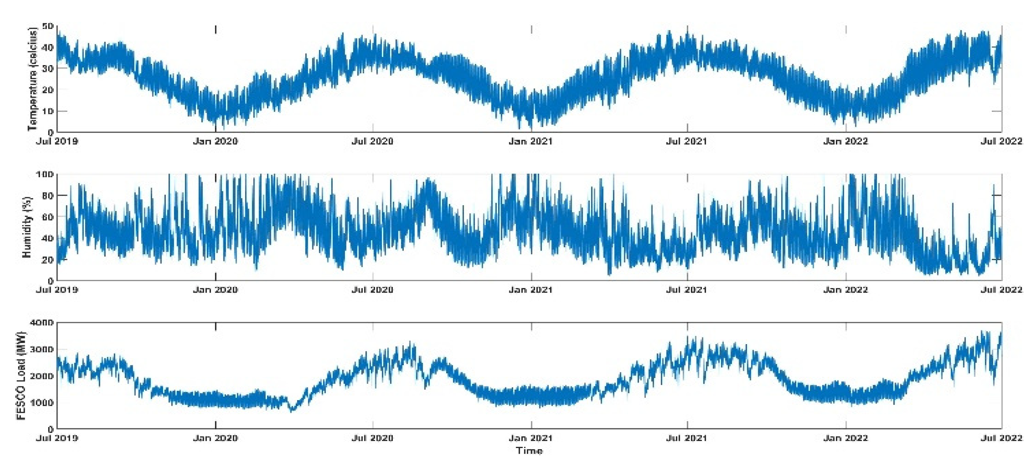
Figure 2.
Data Cleaning of FESCO Load Data.
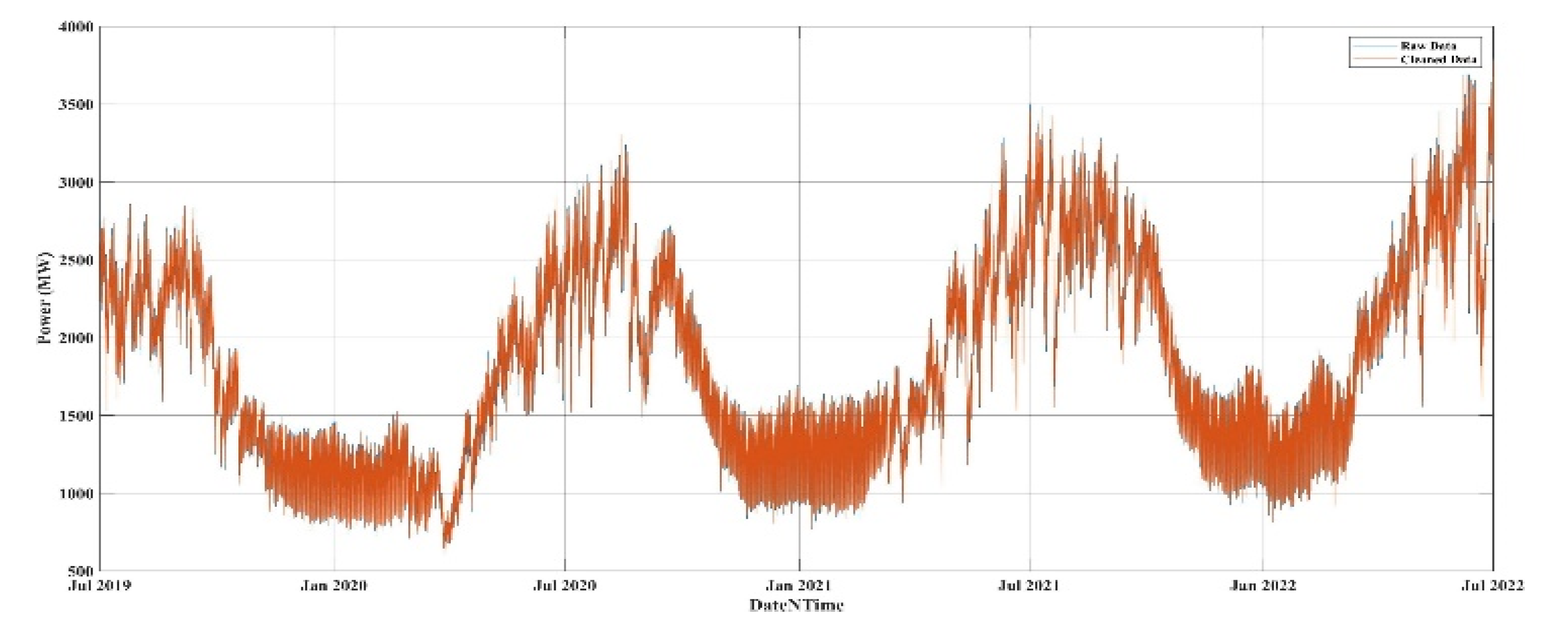
Figure 3.
Autocorrelation of FESCO Data (one month).
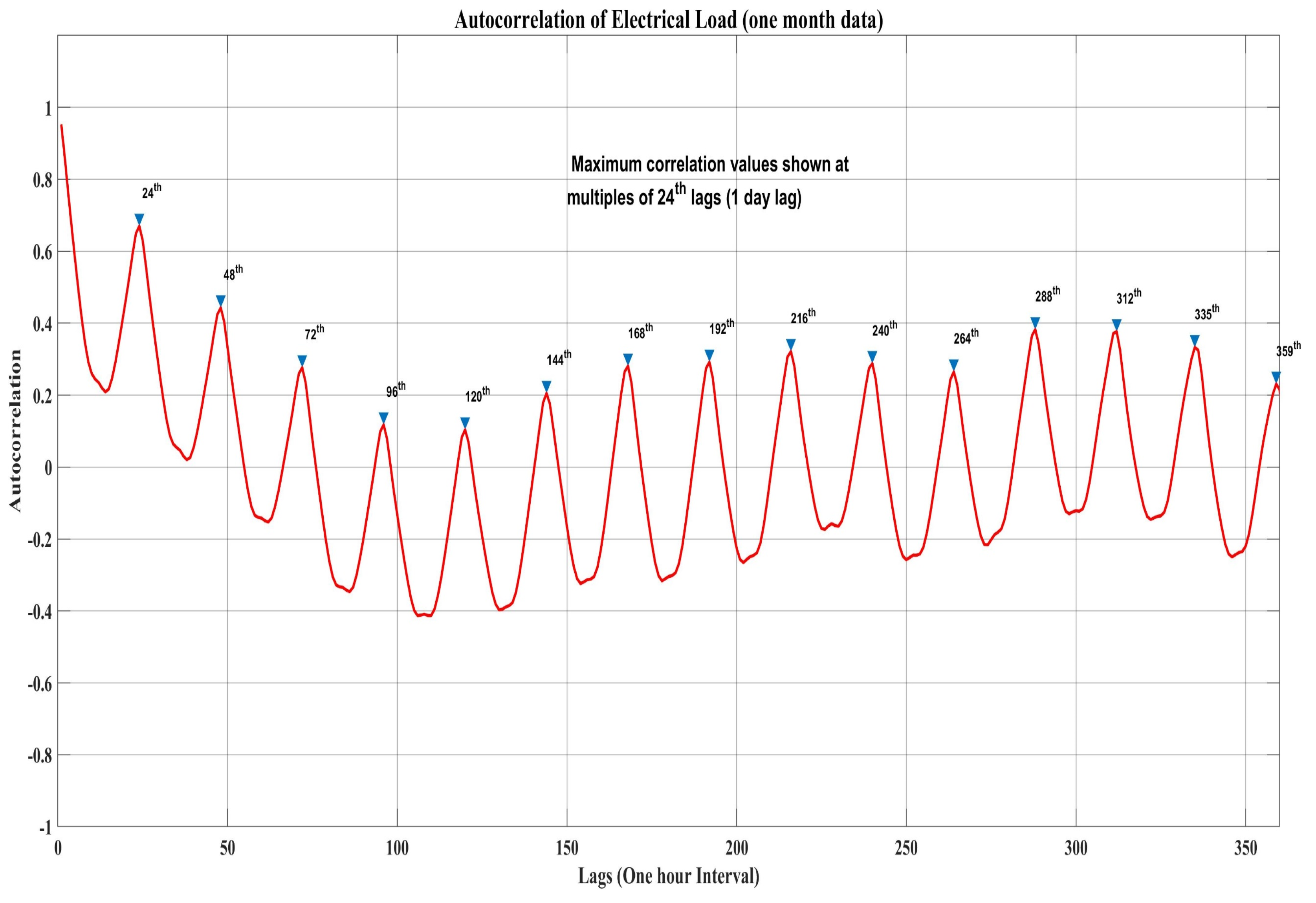
Figure 4.
Figure 4. Autocorrelation of FESCO Data (three-year data).
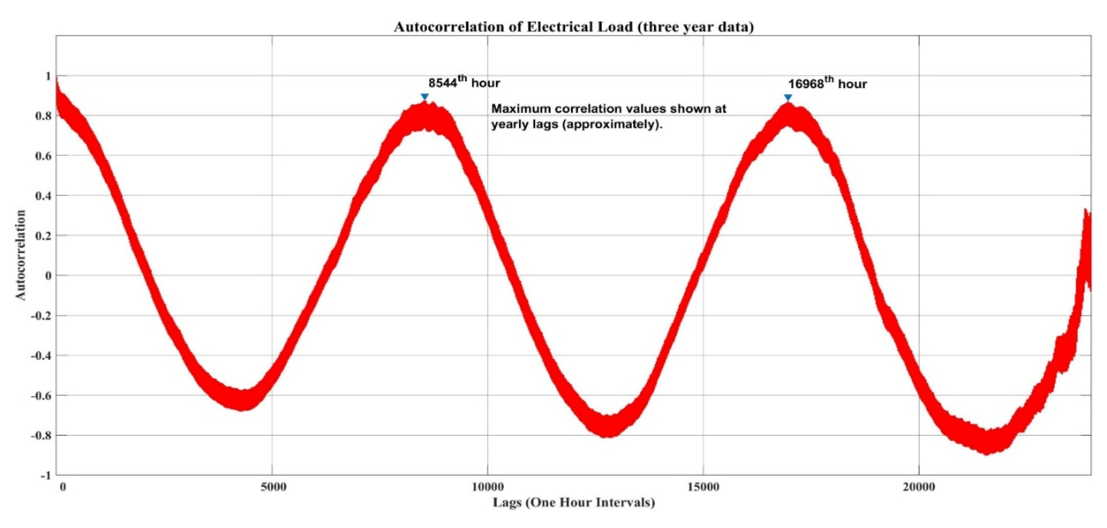
Figure 5.
Electrical Load vs Input Features: (a) & (b)Temperature (c) Humidity (d) h-1 (e) h-2 (f) h-3 (g) h-24 (h) h-48 (i) h-72.
Figure 5.
Electrical Load vs Input Features: (a) & (b)Temperature (c) Humidity (d) h-1 (e) h-2 (f) h-3 (g) h-24 (h) h-48 (i) h-72.
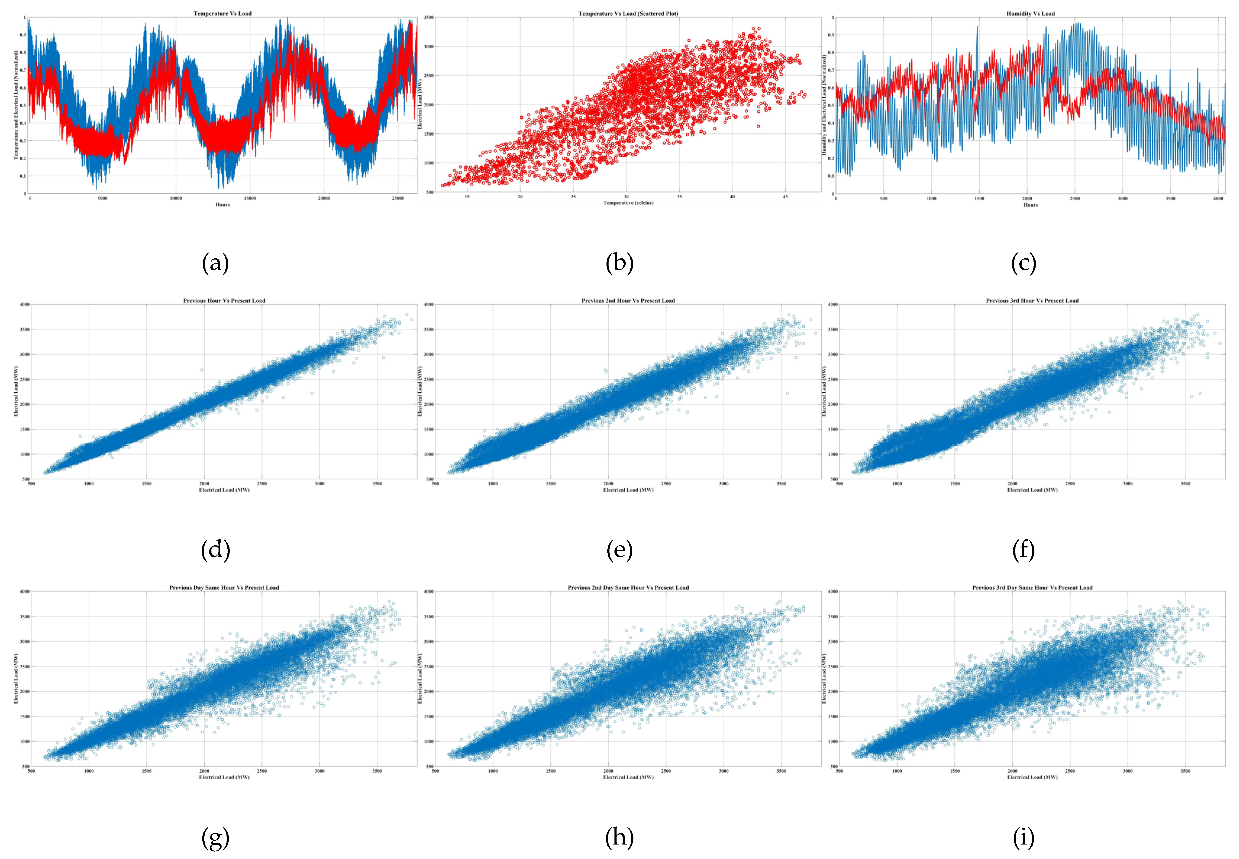
Figure 6.
Performance Metrics comparison of different models.
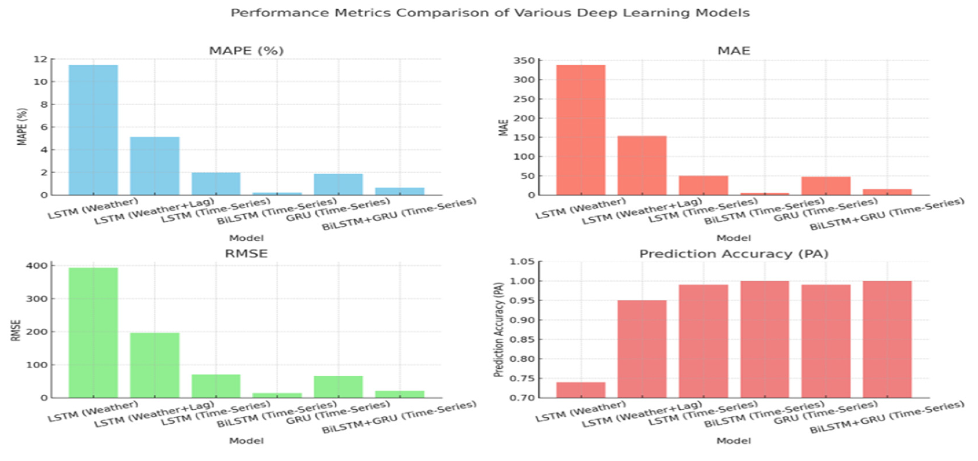
Figure 7.
LSTM Prediction Graph (data as timeseries).
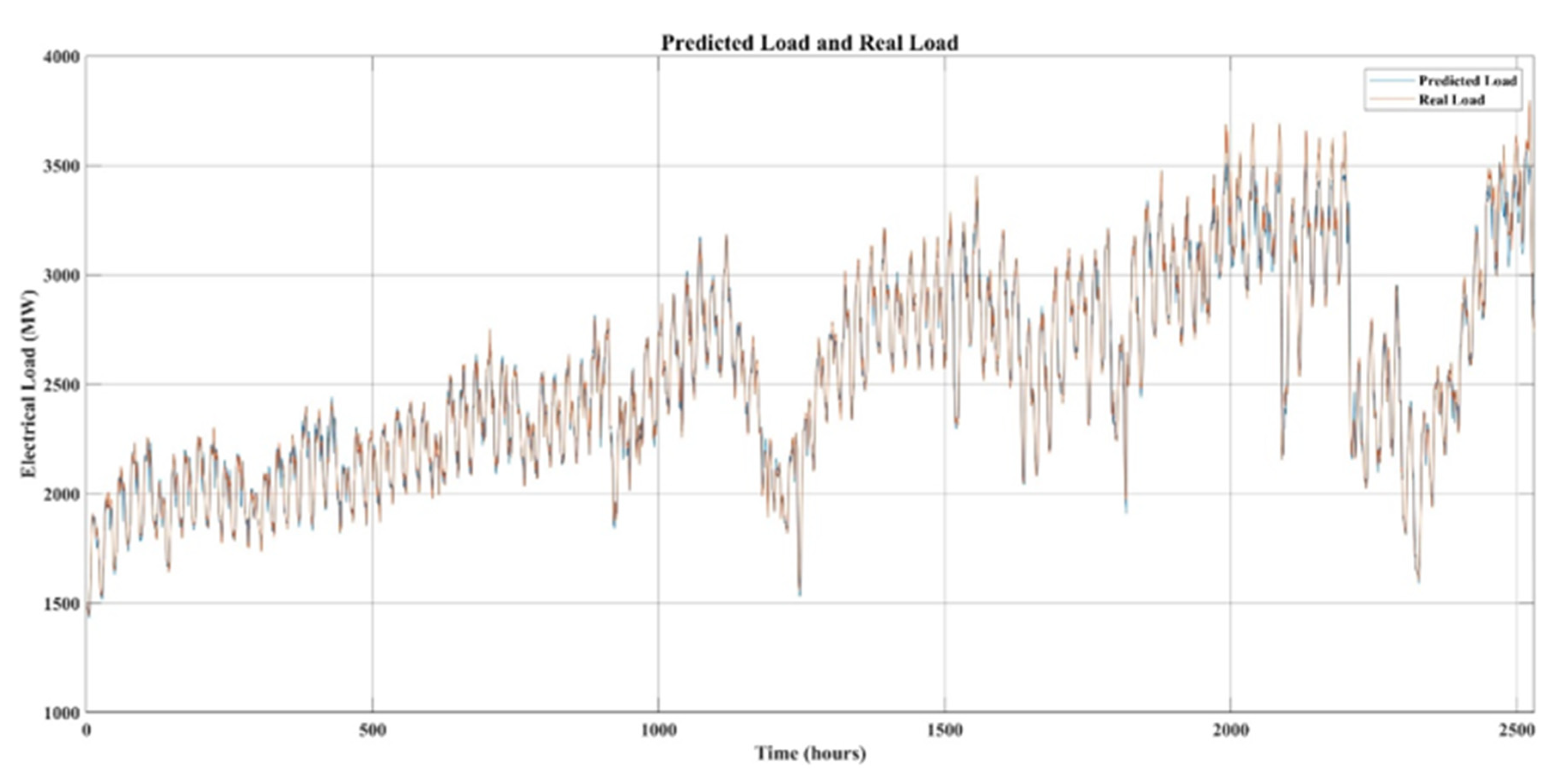
Figure 8.
GRU Prediction Graph (data as timeseries).
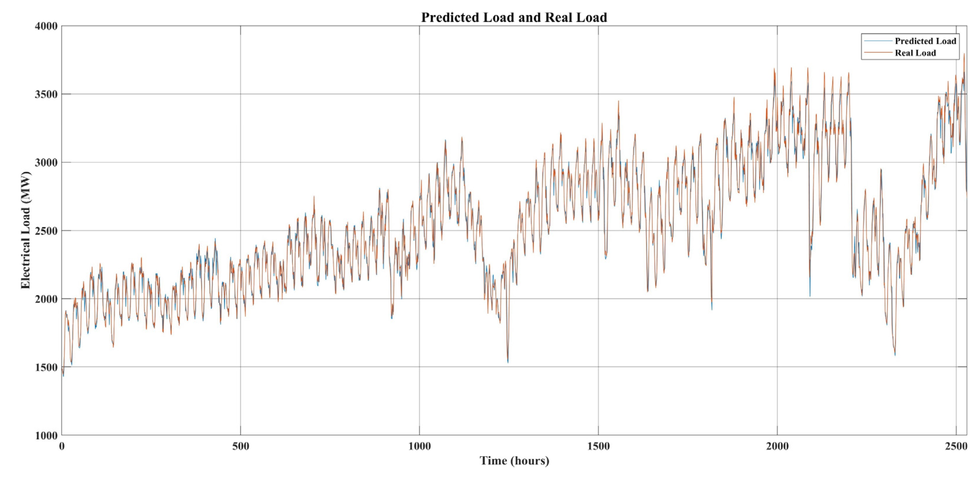
Figure 9.
BiLSTM-GRU Prediction Graph (data as timeseries).
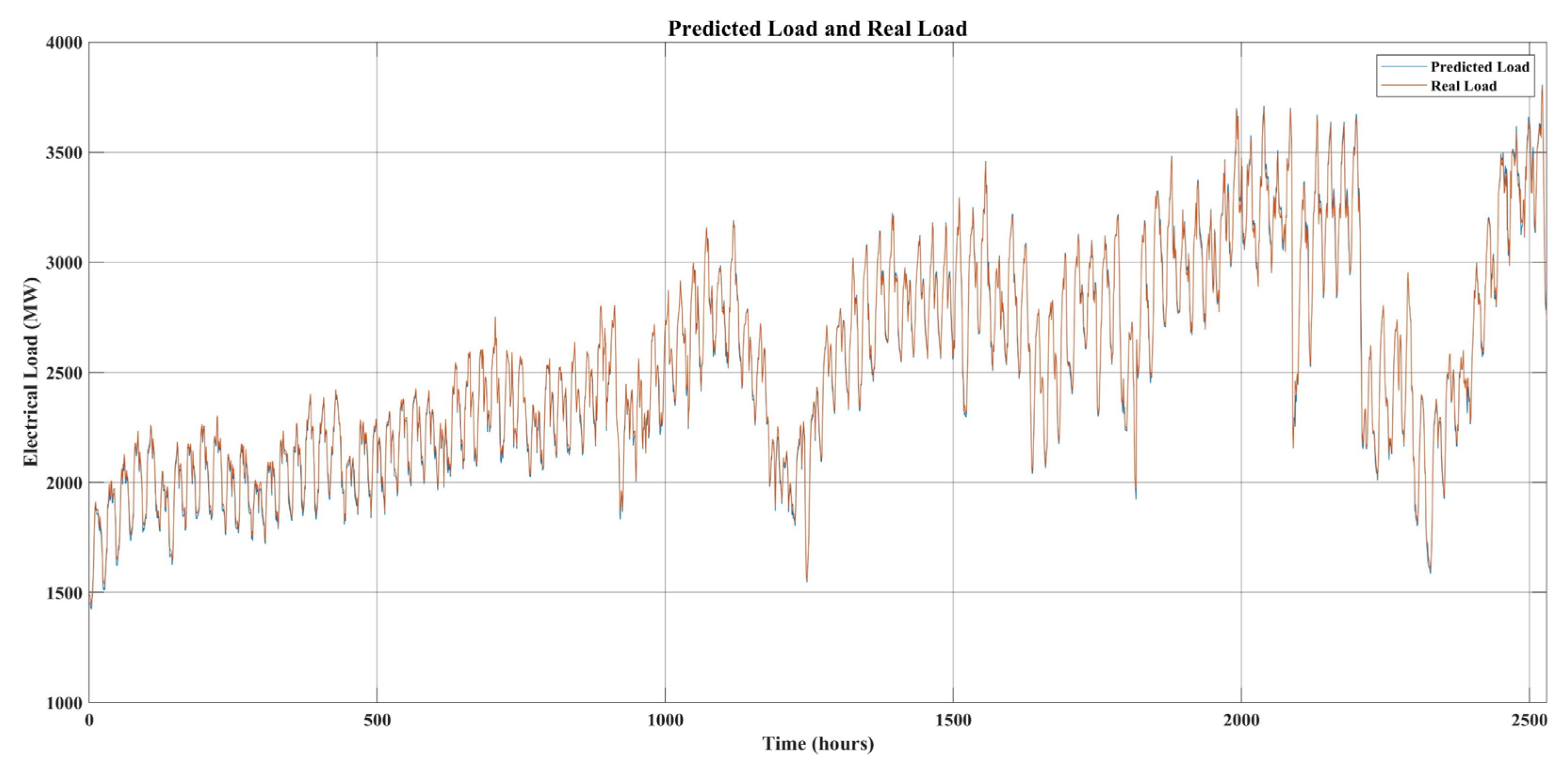
Figure 10.
BiLSTM Prediction Graph (data as timeseries).
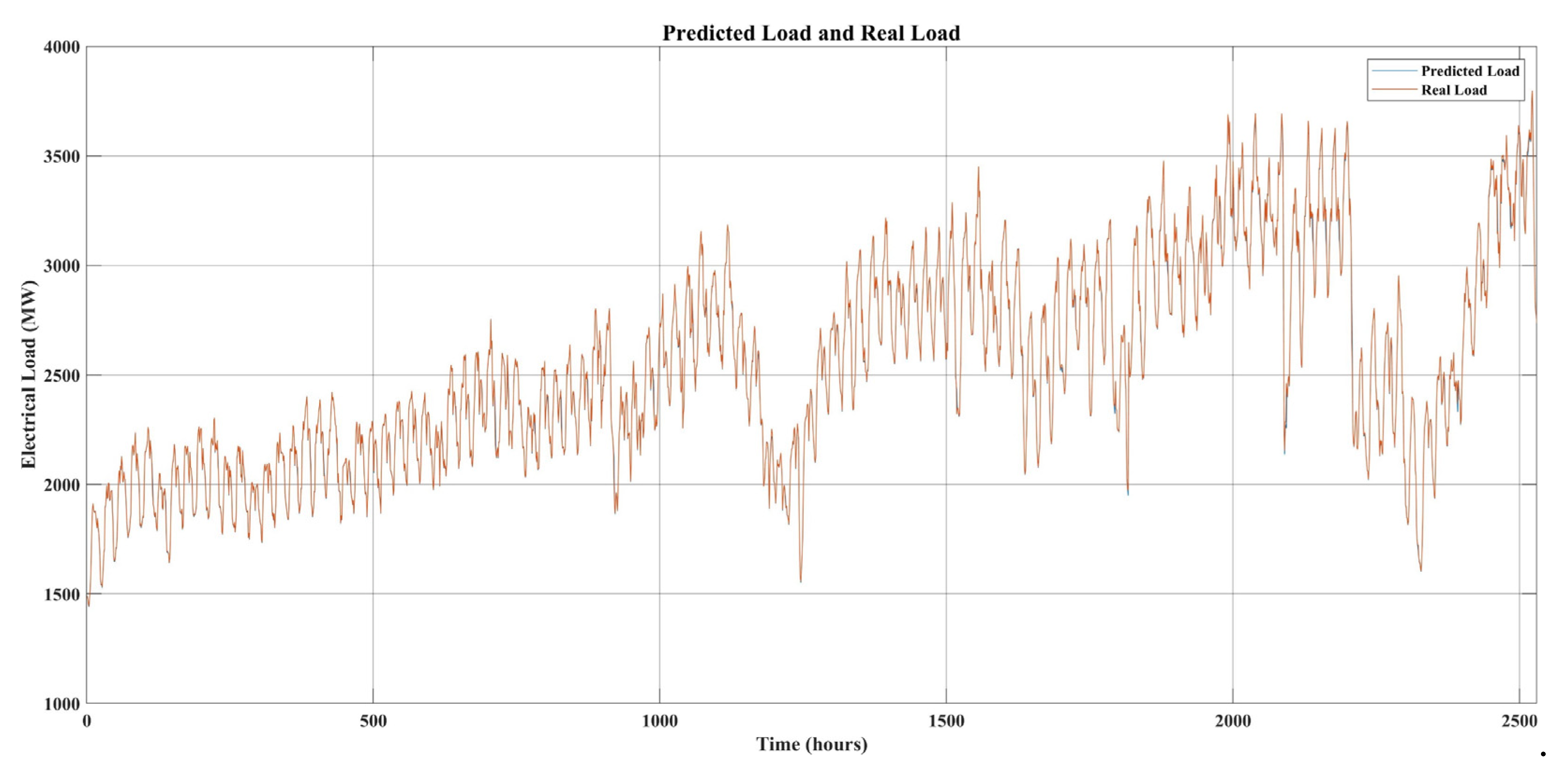
Figure 10.
Performance metrics comparison of BiLSTM on monthly data.
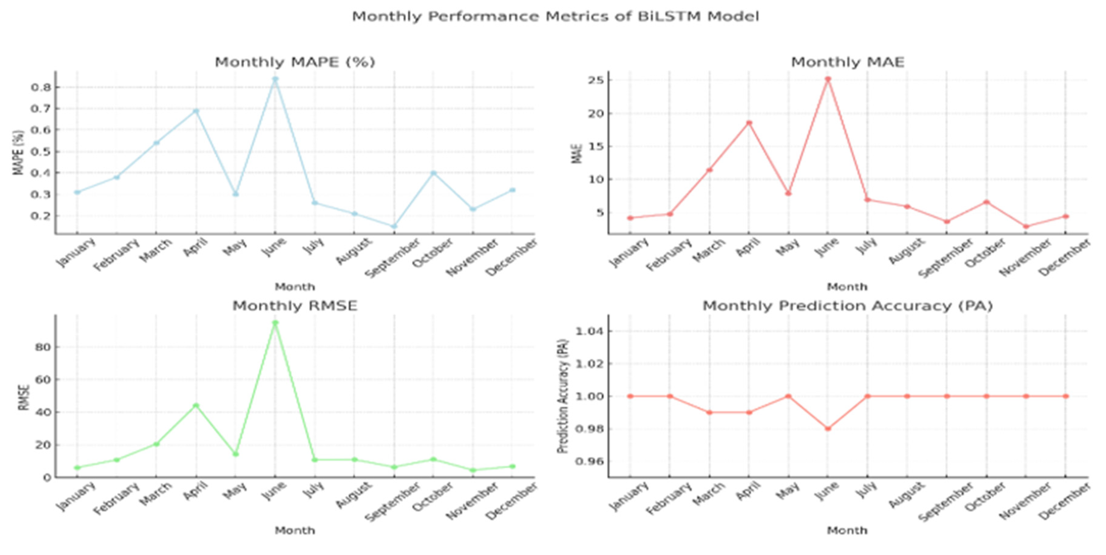
Figure 11.
Lowest MAPE % of the proposed model.
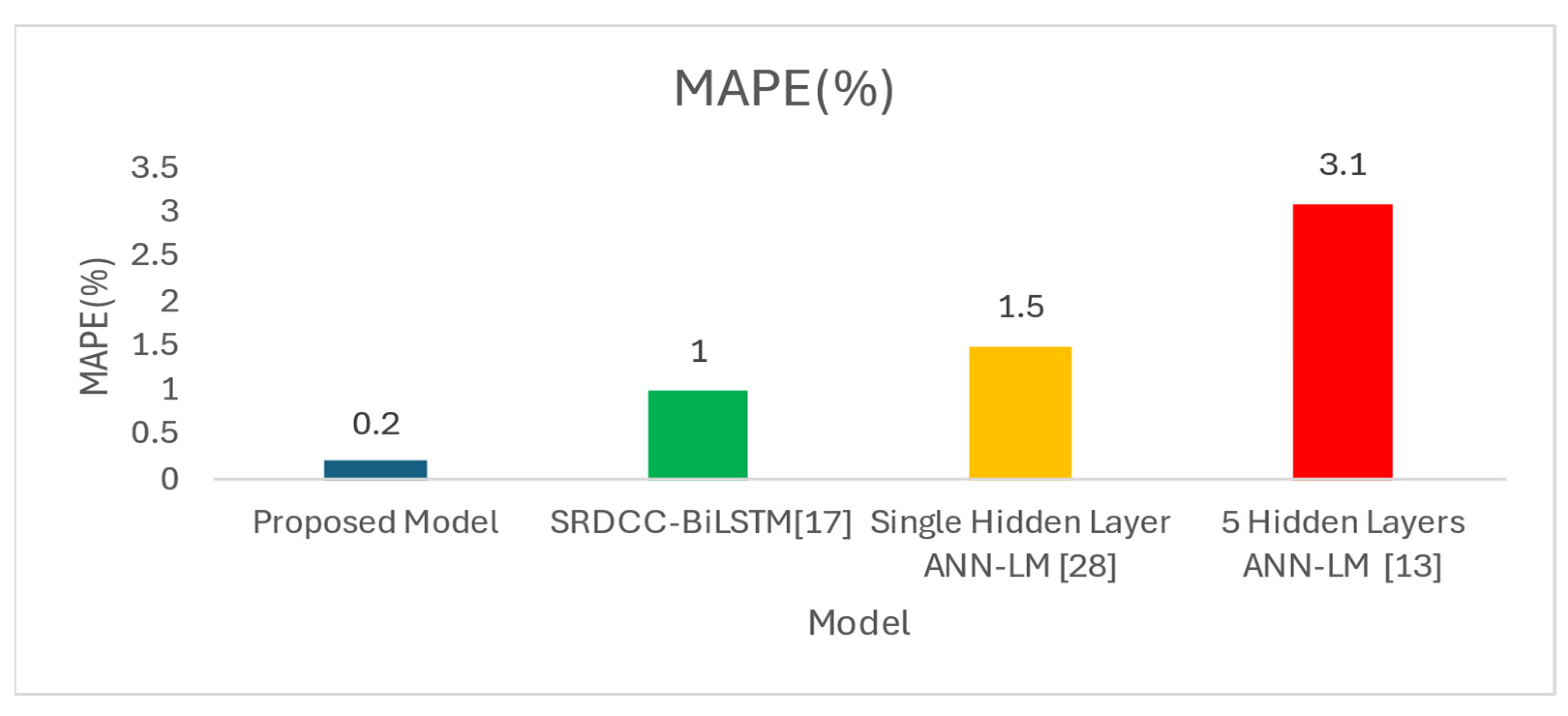
Figure 12.
Lowest MAE of the proposed model.
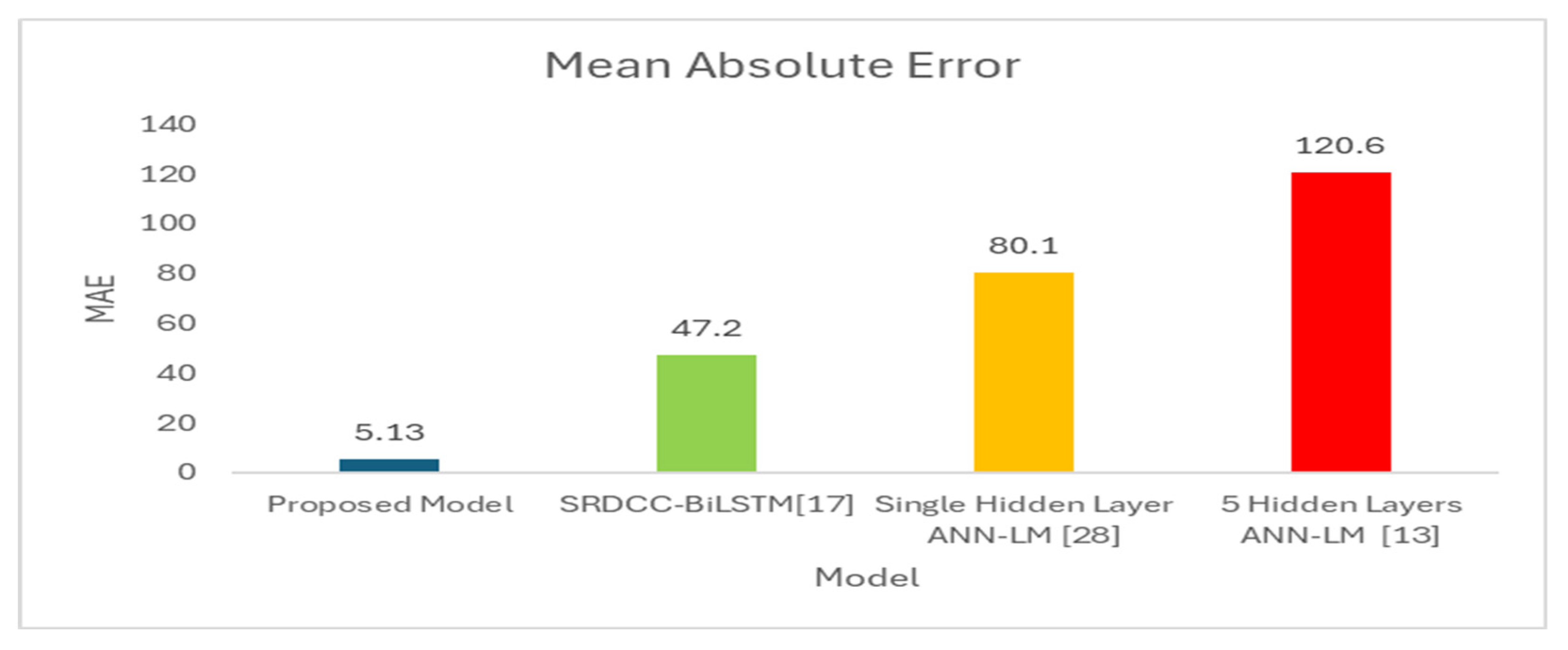
Figure 13.
Lowest RMSE of the proposed model.
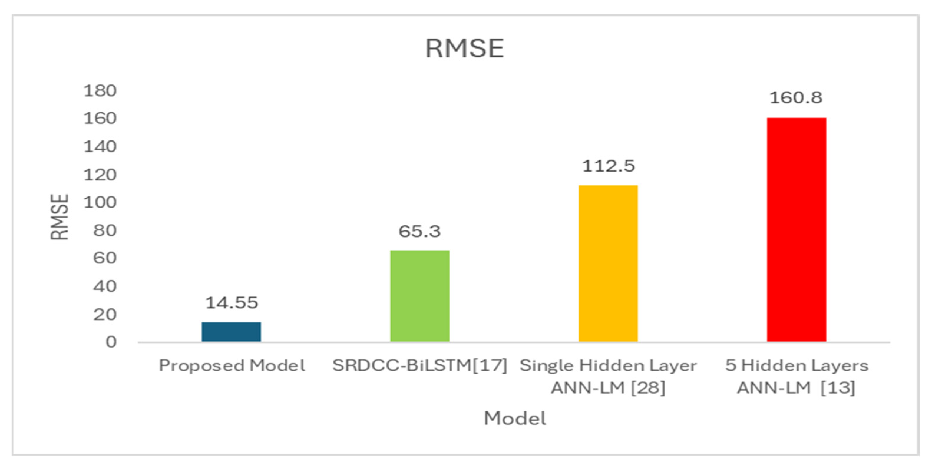
Figure 14.
Highest PA of the proposed model.
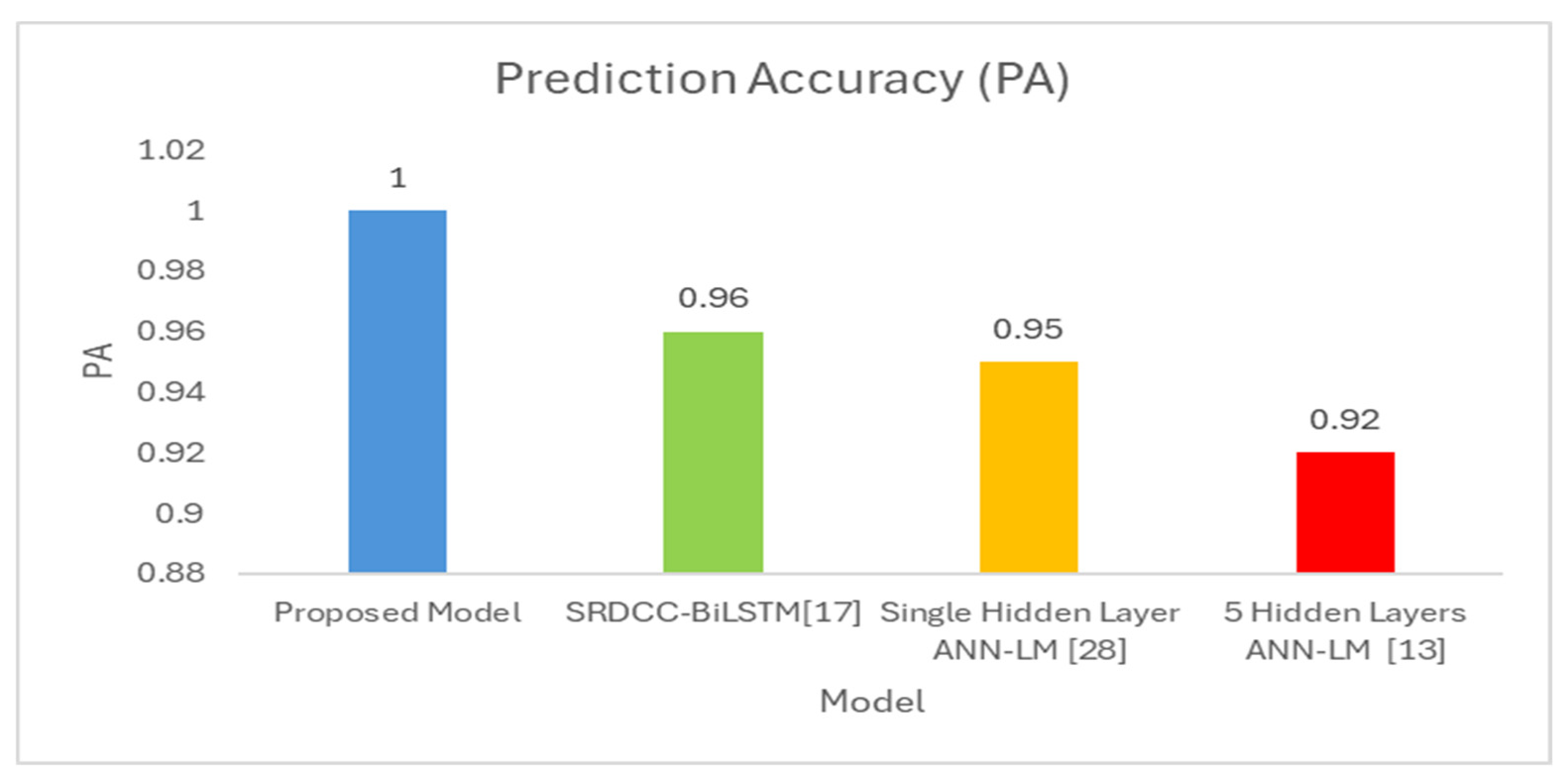

TABLE 1.
SELECTION OF POTENTIAL INPUT PARAMETERS FOR STLF MODELS USING EDA.
| Meteorological Factors | Historical Data |
| Temperature | Previous 1st hour load (h-1) Previous 2nd hour load (h-2) Previous 3rd hour load (h-3) |
| Humidity | Previous 1st day same hour load (h-24) Previous 2nd day same hour load (h-48) Previous 3rd day same hour load (h-72) |
TABLE 2.
PERFORMANCE METRICS COMPARISON OF VARIOUS DEEP LEARNING ALGORITHMS.
| Deep Learning with Input Features (time series) | MAPE | MAE | RMSE | Std.Dev | PA |
|---|---|---|---|---|---|
| LSTM with weather predictors | 11.48 | 338.12 | 392.88 | 6.93 | 0.74 |
| LSTM with weather and lagged predictors | 5.12 | 153.52 | 196.57 | 12.26 | 0.95 |
| Deep Learning without Input Features (time series) | MAPE | MAE | RMSE | Std.Dev | PA |
| LSTM with Time-Series (No Input Feature) | 1.95 | 50.02 | 70.53 | 8.95 | 0.99 |
| BiLSTM with Time-Series (No Input Feature) | 0.20 | 5.13 | 14.55 | 9.22 | 1.00 |
| GRU with Time-Series (No Input Feature) | 1.87 | 47.55 | 66.39 | 9.06 | 0.99 |
| BiLSTM+GRU with Time-Series (No Input Feature) | 0.64 | 15.43 | 21.60 | 9.47 | 1.00 |
TABLE 3.
PERFORMANCE METRICS OF BILSTM DEEP LEARNING ALGORITHMS (MONTHLY MODELS).
| Monthly BiLSTM Model | MAPE | MAE | RMSE | Std.Dev | PA |
| BiLSTM with Time-Series (January) | 0.31 | 4.15 | 5.99 | 13.70 | 1.00 |
| BiLSTM with Time-Series (February) | 0.38 | 4.71 | 10.79 | 16.73 | 1.00 |
| BiLSTM with Time-Series (March) | 0.54 | 11.39 | 20.49 | 10.53 | 0.99 |
| BiLSTM with Time-Series (April) | 0.69 | 18.57 | 44.25 | 19.47 | 0.99 |
| BiLSTM with Time-Series (May) | 0.30 | 7.84 | 14.21 | 18.98 | 1.00 |
| BiLSTM with Time-Series (June) | 0.84 | 25.25 | 95.24 | 36.56 | 0.98 |
| BiLSTM with Time-Series (July) | 0.26 | 6.89 | 10.84 | 18.40 | 1.00 |
| BiLSTM with Time-Series (August) | 0.21 | 5.88 | 10.96 | 15.36 | 1.00 |
| BiLSTM with Time-Series (September) | 0.15 | 3.60 | 6.32 | 16.39 | 1.00 |
| BiLSTM with Time-Series (October) | 0.40 | 6.55 | 11.05 | 11.48 | 1.00 |
| BiLSTM with Time-Series (November) | 0.23 | 2.84 | 4.43 | 14.75 | 1.00 |
| BiLSTM with Time-Series (December) | 0.32 | 4.39 | 6.76 | 17.08 | 1.00 |
Disclaimer/Publisher’s Note: The statements, opinions and data contained in all publications are solely those of the individual author(s) and contributor(s) and not of MDPI and/or the editor(s). MDPI and/or the editor(s) disclaim responsibility for any injury to people or property resulting from any ideas, methods, instructions or products referred to in the content. |
© 2026 by the authors. Licensee MDPI, Basel, Switzerland. This article is an open access article distributed under the terms and conditions of the Creative Commons Attribution (CC BY) license.
Copyright: This open access article is published under a Creative Commons CC BY 4.0 license, which permit the free download, distribution, and reuse, provided that the author and preprint are cited in any reuse.


