
Submitted:
10 June 2025
Posted:
11 June 2025
You are already at the latest version
Abstract
In this study, we consider mid-term load forecasting which is essential for energy infrastructure planning and investment. This study focuses on the Texas power grid, where electricity consumption has surged due to rising industrial activity and rapid data center expansion. Based on an extensive exploratory data analysis, we identify key characteristics of monthly electricity demand in Texas, including an accelerating upward trend, strong seasonality, and temperature sensitivity. In response, we propose a regression-based forecasting model that incorporates a carefully designed set of input features, including a nonlinear trend, lagged demand variables, a seasonality-adjusted month variable, average temperature of a representative area, and calendar-based proxies for industrial activity. The model is trained on monthly data from 2013 to 2023 and tested in 2024. Comparative experiments against benchmarks including Holt-Winters, SARIMA, Prophet, RNN, LSTM, Random Forest, LightGBM, and XGBoost, show that the proposed model achieves superior performance with a mean absolute percentage error of approximately 2%. The results indicate that a well-structured regression approach can effectively outperform several advanced machine learning methods in mid-term load forecasting.
Keywords:
mid-term load forecasting
; energy demand
; regression model
; data centers
; Texas power system
1. Introduction
The electricity load forecasting problem plays a fundamental role in the efficient operations of power systems. Accurate load forecasting is known to be essential for saving investment costs and providing better scheduling for the development of power plants, distribution and transmission grids [1]. Load forecasting is commonly categorized by its time horizon: long-term (a year to several years or decades), mid-term (several months to a year), short-term (hourly, daily, weekly), and very short-term (less than an hour) [2]. Forecasts with a shorter time horizon are vital for real-time system operations, unit scheduling, and demand response, while forecasts with a longer time horizon are critical for strategic managerial decisions, such as infrastructure expansion planning and determining investments in power plants and grid development.
In recent years, electricity demand has become increasingly influenced by emerging technological trends beyond traditional drivers such as weather patterns, calendar effects, and economic conditions. The rapid advancement of generative artificial intelligence (AI) and the widespread deployment of large language models (LLMs) have accelerated the construction and operation of energy-intensive data centers. According to the International Energy Agency, a single AI-focused data center can consume as much electricity as 100,000 households, with the largest facilities under construction expected to consume as much power as up to 2 million households [3]. This phenomenon is driving a structural transformation in electricity load patterns, especially in regions where data center investments are heavily concentrated. The global electricity demand from data centers is projected to continue increasing, with AI identified as the most significant contributor to this increase.
In this study, we focus on one of the regions most affected by the rise of data centers, namely, Texas. Texas is one of the top three data center hubs in North America, alongside Virginia and California [4]. More importantly, the state's power system is managed by a single, independent operator—ERCOT (Electric Reliability Council of Texas)—which governs approximately 90% of the state's electric load. ERCOT's centralized structure allows forecasting outcomes to be directly linked to operational and planning decisions. The construction of data centers in Texas is expected to continue due to several reasons including relatively low-cost electricity, tax incentives, a business-friendly environment, excellent network connectivity, and access to renewable energy sources [5]. Therefore, there is a need to develop load forecasting methodologies that account for the anticipated expansion of data centers in the region.
Specifically, this study proposes a method for forecasting mid-term electricity demand in the Texas region. Mid-term forecasts are particularly valuable for decisions related to capacity planning, procurement, and infrastructure investment, which bridges the gap between short-term operational planning and long-term strategic investments [6]. This is particularly important in the context of rising data center electricity consumption, which causes substantial increases in load demand, because the expansion of generation and transmission infrastructure becomes inevitable as a response to such growing demand. Considering the lead time required to build such infrastructure, accurately forecasting electricity demand over a mid-term horizon is therefore essential.
Despite its practical significance, mid-term load forecasting (MTLF) has traditionally received less attention in academic literature. As noted in the survey by Kuster et al. [2], the proportion of studies devoted to mid-term forecasting is considerably lower than for short-term or long-term forecasting. However, a substantial number of MTLF studies have been conducted, to the extent that comprehensive review articles have been published focusing on this forecasting horizon [6]. Several recent MTLF studies illustrate the increasing research interest in this domain. Sharma and Jain [7] utilized monthly load data from Madhya Pradesh, India and introduced a two-stage framework incorporating neural network schemes. Rubasinghe et al. [8] proposed a hybrid CNN-LSTM to forecast monthly load of New South Wales, Australia. Li et al. [9] used monthly electricity consumption data from China and proposed ISSA-SVM, where Support Vector Machine is optimized by an Improved Sparrow Search Algorithm. Dudek and Pelka [10] collected monthly electricity demand data from 35 European countries and forecasted 12-month demand of 2014 using Pattern Similarity-based Methods. Oreshkin et al. [11] also covered European countries’ monthly electricity demand. They forecasted 12-month demand of 2013 using N-BEATS deep neural network architecture. A common feature observed across these recent studies is their use of monthly data to perform MTLF across diverse geographical regions. Moreover, the proposed methods in these studies consistently achieved mean absolute percentage errors (MAPEs) around 3%. In this study, we focus on a region that has not been explicitly addressed in the studies—North America, and more specifically Texas. We propose an MTLF method that is designed to achieve a MAPE below 3%.
Electricity demand forecasting studies on Texas have notably surged since the 2021 blackout by winter storm Uri. According to Popik and Humphreys [12], the blackout was caused by factors including demand levels exceeding ERCOT's peak forecasts, widespread generation outages across multiple energy sources, etc. As a result, research into Texas’s electricity load forecasting has grown significantly, while most existing studies have concentrated on short-term load forecasting. Table 1 summarizes selected recent studies on electricity demand forecasting in Texas.
As presented above, many studies have been conducted in response to the growing need for load forecasting in the Texas region, particularly following the 2021 blackout. However, there remains a lack of research targeting MTLF for this region. This study proposes an MTLF framework tailored to the Texas power grid. Specifically, the model is trained on monthly electricity load and related data from 2014 to 2023, with the aim of forecasting demand for each month of 2024. The remainder of this paper is organized as follows. The next section presents the exploratory data analysis to explore the characteristics of electricity demand and influencing factors on the demand. Section 3 introduces the proposed forecasting methodology in this study. In Section 4, comparative analysis is carried out to validate the performance of the proposed method against existing methods. Finally, Section 5 concludes the study with a summary of key findings and suggestions for future research directions.
2. Data Analysis
To enhance the accuracy of electricity load forecasting, it is essential to first understand the characteristics of electricity demand in the Texas region from multiple perspectives. This section also explores various factors affecting the Texas grid to identify exogenous variables that influence its electricity demand. By analyzing these characteristics, we seek to provide meaningful insights that can improve the design of the forecasting model. In this study, net electricity generation data for Texas were collected from the U.S. Energy Information Administration (EIA) via its public data portal (https://www.eia.gov/electricity/data/browser/) and used to represent electricity demand. Figure 1 shows a time series plot (in 1,000 MWh) of monthly electricity demand in Texas from 2013 to 2023.
As you can see from Figure 1, several key temporal characteristics of the time series are revealed. First, the demand exhibits a modest upward trend over the ten-year span. Notably, after 2020, the overall demand level seems to increase more markedly. This shift may be attributed to the installations of new demand centers. Second, a strong seasonal pattern is observed, with electricity demand repeatedly peaking during the summer months as well as relatively small peaks during the winter months. Lastly, increasing volatility is observed in recent years (2021–2023), with greater amplitude observed in monthly demand variations. This trend may reflect growing complexity in the Texas electricity system, driven by factors such as weather anomalies, grid constraints, and rising electricity demand from non-traditional sources like AI-driven data centers. These characteristics address the need for forecasting models that can effectively accommodate an upward trend, seasonality, and increasing volatility.
To more clearly capture the seasonal characteristics of electricity demand in Texas, Figure 2 shows the monthly average electricity consumption for each calendar month from 2013 to 2023. As shown in the figure, electricity demand varies significantly throughout the year, confirming the presence of strong intra-annual seasonality. The highest average demand occurs during the summer months, i.e., July and August. This seasonal peak is largely attributable to increased use of air conditioning during hot summers. During the winter season, electricity demand tends to rise in January and December, however, the magnitude of demand in these months remains lower than that observed in June and September. This indicates that while heating needs may contribute to increased consumption during colder months, their impact is less pronounced than the cooling-driven spikes observed in the summer. The following figure shows the relationship between electricity demand and temperature of the Texas region.
Figure 3 displays a scatter plot illustrating the relationship between monthly electricity demand and average temperature in Texas. Each point represents a single month from 2013 to 2023, and the color gradient indicates the corresponding year, with darker tones representing earlier years and lighter tones representing more recent years. Temperature data are based on monthly averages from Dallas—the most populous city in Texas—and were obtained from the website of National Weather Service (https://www.weather.gov/wrh/Climate?wfo=ewx). The plot reveals a distinct convex nonlinear relationship between average temperature and electricity demand. Specifically, electricity consumption tends to be relatively moderate in the mid-temperature range, while it increases at both ends of the temperature scale. However, the convex relationship is notably asymmetric, with a sharper increase in electricity demand at higher temperatures than it does at lower temperatures. As the years progress, electricity demand shows a general upward trend; however, the asymmetric convex relationship with temperature remains consistent throughout the period.
Figure 4 presents the autocorrelation function (ACF) plot of monthly electricity demand in Texas, providing insights into the temporal dependence structure of the time series. As observed in the figure, electricity demand exhibits strong autocorrelation at lag 1 and significant spikes in autocorrelation are evident at 12-month intervals, suggesting the presence of annual seasonality in the data. These findings imply that past values—particularly those from the same month in the previous year—contain valuable predictive information. Therefore, incorporating lagged features is likely essential for improving the accuracy of mid-term load forecasting models.
Thus far, we have confirmed typical characteristics of monthly electricity demand, including upward trends, seasonal fluctuations, autocorrelations, and their relationship with temperature. As a final component of this section, we turn our attention to the geo-economic context of Texas. As noted earlier, Texas has emerged as one of the most active regions for data center construction. In addition to digital infrastructure, the state continues to attract a diverse array of businesses, electrify oil and gas operations, and so on. These changes have collectively led to a sharp increase in industrial electricity demand [22]. The following figure presents a visualization that allows for indirect observation of the relationship between industrial activity and electricity demand.
To indirectly capture the intensity of industrial activity in Texas, this study first considers the number of working days in each month as a proxy indicator. Figure 5(a) illustrates the average monthly electricity demand grouped by the month length (28 to 31 days). The figure shows a clear positive relationship: months with more days tend to exhibit higher electricity demand. This suggests that longer months may correspond to greater levels of economic and industrial activity, which in turn contribute to increased power consumption. It is worth noting that July and August also have 31 days, which may further reinforce this pattern. Figure 5(b) presents the relationship between the number of weekday holidays in a given month (as defined by federal and Texas state holidays) and average electricity demand. As the number of weekday holidays increases, a general decline in electricity consumption is observed. This inverse relationship supports the hypothesis that reduced working days are associated with lower levels of industrial and commercial electricity usage. These results indicate that calendar-based variables can serve as meaningful proxies for industrial activity and need to be incorporated into the forecasting model.
3. Methodology
This study proposes a regression-based framework for forecasting monthly electricity demand in the Texas region. The predictive performance of such a model is heavily dependent on the selection and construction of input variables. As discussed in the previous section, Texas’s electricity demand exhibits distinct temporal patterns—such as trend, seasonality, and autocorrelation—as well as sensitivity to exogenous factors including temperature and industrial activity. Therefore, effectively translating these influences into well-structured input variables is essential for enhancing model accuracy. Although regression is a traditional forecasting approach, when properly designed with domain-specific variables, it can outperform more complex machine learning techniques. This section is organized as follows: Subsection 3.1 outlines the input variables used in the model, and Subsection 3.2 introduces the proposed regression model.
3.1. Input Variables
3.1.1. Trend
A common approach to capturing trend effects in time series forecasting models is to include a time index as an input variable. Since this study focuses on monthly data, the time index t is defined such that January 2013 (the beginning of the training period) corresponds to t=1, and increases by one each month, reaching t=132 in December 2023. Including this index as a variable in the model allows for the representation of linear trends in electricity demand. However, as observed in Figure 1, electricity demand in Texas has exhibited an accelerating upward trend in recent years, especially due to the expansion of data centers and industrial activity. This suggests that a nonlinear trend specification is more appropriate. To account for this, we include squared term t2 as an input variable.
3.1.2. Autocorrelations
As identified in the ACF plot shown in Figure 4, monthly electricity demand in Texas exhibits strong temporal dependence, particularly with the immediately preceding month and the same month of the previous year. To reflect this autocorrelation structure, the forecasting model should include lagged demand variables as predictors. Let yt denote the electricity demand at time t, which serves as the dependent variable in our model. To capture autocorrelative effects, the values of yt−1 and yt−12 would be considered as relevant input variables. However, in the context of mid-term forecasting, incorporating the immediately preceding month’s demand (yt−1) may not be feasible or appropriate, as future values are predicted multiple months ahead. As an alternative, this study adopts yt−13, the electricity demand from the month prior to the same month last year, as a substitute variable. This lag still retains meaningful predictive power, as evidenced by its statistically significant autocorrelation in Figure 4.
3.1.3. Seasonality
Incorporating lagged demand from the same month of the previous year (i.e., yt−12) reflects the autocorrelation as mentioned earlier but also partially captures seasonal effects. However, to explicitly represent seasonality, this study also includes a month indicator variable as an additional input feature. Let mt denote the month corresponding to time t. There are generally two approaches to including this variable in a model. The first is to treat mt as a categorical variable, where, for example, January 2013 would be encoded as “January” and December 2023 as “December.” While this approach accurately represents monthly seasonality, it requires the use of 11 dummy variables to encode 12 months, which increases model complexity and may lead to sparsity issues. Alternatively, the month variable can be treated as a numerical variable, where January is coded as 1, February as 2, ..., and December as 12. Although this encoding assumes a linear ordering of months, empirical studies and practical applications often show that this simplification yields comparable performance to categorical encoding.
This study proposes a new formulation of the month variable, to leverage the strengths of both approaches while mitigating their respective limitations. Specifically, instead of encoding months in calendar order (i.e., January = 1, ..., December = 12), we assign numeric values to months based on their average electricity demand, as observed in train data. This approach retains the computational simplicity of a numeric variable, while embedding domain-relevant seasonal information directly into the feature. Figure 6 illustrates the average electricity demand for each calendar month from 2013 to 2023, sorted in ascending order.
In this study, we assign the modified month variable according to the ascending order of average monthly electricity demand as shown in Figure 6. For example, February is assigned a value of 1, April is assigned 2, and August is assigned a value of 12. In summary, modified month variables mt for t=1, 2, 3, 4, 5, 6, 7, 8, 9, 10, 11, and 12 have values 7, 1, 3, 2, 8, 10, 11, 12, 9, 5, 4, and 6, respectively. This reordering embeds the demand intensity of each month into a single numeric variable, allowing the model to better capture seasonal variation while avoiding the dimensionality inflation associated with dummy encoding
3.1.4. Temperature
As observed in Figure 3, there exists a clear nonlinear relationship between electricity demand and temperature in Texas. To capture this effect, it is essential to include temperature variables in the model. However, a challenge arises from the geographical diversity of the state—temperature varies across different regions. The National Weather Service provides monthly average temperature data for major Texas regions, including Dallas, Houston, Austin, and San Antonio. To determine the most representative temperature input for the model, this study first computes the Pearson correlation coefficients between monthly electricity demand and the average temperatures of each city. In addition, we calculate the correlation between electricity demand and the average of the four cities' temperatures, treating it as a potential aggregate indicator. The results are summarized in Table 2 below.
As shown in Table 2, all four cities exhibit strong positive correlations between monthly electricity demand and average temperature. Among them, Dallas has the highest correlation coefficient, suggesting that temperature fluctuations in Dallas are most closely aligned with variations in statewide electricity demand. This may be attributed to Dallas being the most populous city in Texas and a central hub for data center development, both of which significantly influence total electricity usage. Based on these results, this study selects the average monthly temperature of Dallas as the representative temperature variable in the proposed forecasting model and other cities’ temperature values are excluded to prevent multicollinearity.
3.1.5. Other Features
As the final set of input variables, this study includes two calendar-based features introduced in the previous section: the total number of days in a month and the number of weekday holidays. Let dt denote the number of calendar days in month t, and ℎt represent the number of weekday holidays in the same month. These variables are intended to serve as proxies for industrial activity, which is a key driver of electricity demand. While it is theoretically possible to incorporate direct measures of industrial output or sector-specific electricity consumption, doing so poses several challenges—most notably, limited data availability and the impracticality of knowing future values for predictive purposes. In contrast, both dt and ℎt are deterministic calendar attributes that can be easily known in advance for any future time point, making them especially suitable for forecasting tasks. By incorporating these two variables, the proposed model can reflect the expected monthly variation in electricity demand driven by the operational intensity of industrial and commercial sectors.
3.2. Proposed Regression Model
Building upon the input features discussed in the previous subsection, this study proposes a multiple linear regression model to forecast monthly electricity demand in Texas. The model aims to capture both temporal and exogenous influences using a structured and interpretable set of input variables. The functional form of the proposed regression model, which regresses monthly electricity demand yt, is expressed as:
, where:
𝑦𝑡=𝛽0+𝛽1𝑡2+𝛽2𝑦𝑡−12+𝛽3𝑦𝑡−13+𝛽4𝑚𝑡+𝛽5T𝑡+𝛽6𝑑𝑡+𝛽7ℎ𝑡+𝛽8(T𝑡⋅𝑑𝑡)+𝜖𝑡
t is the time index representing the upward trend of the monthly electricity demand;
yt−12 is the electricity demand from the same month in the previous year of the t-th month;
yt−13 is the electricity demand from the month prior to the same month last year of the t-th month;
mt is the modified month variable at the t-th month in such that if the month of t-th month are January, February, March, April, May, June, July, August, September, October, November, and December, then mt are 7, 1, 3, 2, 8, 10, 11, 12, 9, 5, 4, and 6, respectively;
Tt is the average monthly temperature in Dallas at the t-th month;
dt is the number of days at the t-th month;
ht is the number of weekday holidays at the t-th month;
βi represents the coefficient of i-th term of the model, for i=1, 2, …, 8;
and ϵt denotes the error term.
All terms from the first to the seventh in the proposed model (i.e., β1t2 to β7ℎt) directly correspond to the input variables introduced in Subsection 3.1, so it is not hard to understand. However, the final term, the interaction between average temperature and the number of days in a month (β8(Tt⋅dt)), might need additional explanation. As shown in Figure 3, electricity demand rises more sharply at higher temperature levels, suggesting a nonlinear amplification effect. That is, the impact of temperature on demand intensifies rather than increases linearly, particularly during hot summer months. To capture this effect, the model introduces an interaction term between temperature and the number of days. This design allows the model to reflect that, for months with both high temperatures and a greater number of days—such as July and August, which each have 31 days—the demand may increase more substantially than in shorter months with similar temperatures. Consequently, this formulation offers interpretability, computational simplicity, and flexibility in capturing key structural patterns of the demand. The adjusted R2 value of the proposed model is 0.921 when fitting the model on train data, which indicates that the proposed model has a sufficient goodness of fit. To assess the statistical significance of each term included in the model, the regression coefficients summary is presented below.
Table 3 summarizes the estimated regression coefficients and associated statistical metrics for the proposed model. Several key findings emerge from this table regarding the contribution and statistical significance of individual predictors. The quadratic time trend variable t2 shows a highly significant positive coefficient, confirming the presence of an accelerating upward trend in electricity demand over time. The lagged demand from the same month in the previous year is also statistically significant, indicating a strong seasonal autocorrelation effect. In contrast, the additional lag variable does not reach conventional levels of significance, suggesting its marginal predictive value may be limited when yt−12 is already included in the model. The modified month variable designed to capture seasonality has a highly significant positive effect. This demonstrates that embedding seasonal intensity directly into the month encoding provides useful information for demand prediction. Interestingly, the coefficient for average temperature is negative and significant which may seem counterintuitive at first. However, this is due to the presence of the interaction term, which has a positive and significant coefficient. This pattern suggests that temperature alone may not adequately explain demand increases unless accompanied by longer durations of exposure—consistent with the heat-load amplification hypothesis discussed earlier. Calendar variables also provide useful insight. The number of days in a month is negatively associated with electricity demand when not interacting with temperature, while the number of weekday holidays is not statistically significant, indicating a weaker or more variable influence on demand during the forecast period. Overall, the regression results confirm that most of the proposed input variables contribute meaningfully to model performance, and the inclusion of nonlinear and interaction effects enhances the model's ability to capture structural characteristics of electricity demand in Texas.
4. Computational Experiments
To evaluate the forecasting performance of the proposed regression model, a series of comparative experiments are conducted against several existing methods. The model is trained using monthly electricity demand data from January 2013 to December 2023, totaling 132 observations. Forecasts are then obtained for the 12 months of 2024 by the forecasting methods, and the accuracy of these forecasts is assessed using three widely used metrics: Mean Absolute Error (MAE), Root Mean Square Error (RMSE), and Mean Absolute Percentage Error (MAPE). The mathematical definitions of each evaluation metric are given as follows:
where represents the actual value at t-th month, denotes the forecasted value at t-th month, n is 144, i.e., the month index of December 2024.
To objectively assess the performance of the proposed model, we compare it with a diverse set of well-known forecasting methods, all trained on the same dataset and used to predict electricity demand for the 12 months of 2024. The benchmark models consist of three univariate time series methods, two neural network-based models, and three machine learning algorithms. First, among the univariate statistical methods, we employ: Holt-Winters, a representative exponential smoothing method capturing level, trend, and seasonal components [23]; SARIMA (Seasonal AutoRegressive Integrated Moving Average), a widely used time series model that incorporates autoregressive, differencing, and moving average terms, along with seasonal components [24]; Prophet, a decomposable model developed by Meta that combines trend, seasonality, and holiday effects [25]. Second, for neural network-based models, we include: Recurrent Neural Network (RNN), which models sequential dependencies through recursive connections and is suitable for temporal data [26]; Long Short-Term Memory (LSTM), a more advanced architecture that mitigates the vanishing gradient problem in RNNs and is particularly effective at capturing long-term dependencies in time series data [27]. Major hyperparameters of RNN and LSTM are set to the same values, such as, optimizer=’adam’, input_shape=(12, 1), dense layer=1, epochs=100, and batch_size=32.
Third, widely used machine learning methods are tested: Random Forest, an ensemble of decision trees that improves prediction accuracy by reducing variance [28]; LightGBM, a gradient boosting framework known for its computational efficiency [29]; XGBoost, another powerful boosting algorithm that incorporates regularization and is widely used in time series and structured data forecasting tasks [30]. All three machine learning methods were trained using the same set of input variables, which include t, yt−12, yt−13, Tt, dt, as used in the proposed model and the original numerical month variable. These benchmark models are chosen to reflect a wide methodological spectrum, ranging from traditional time series analysis to advanced deep learning and machine learning approaches. The results of the computational experiments are summarized in the table below.
Table 4 presents the forecasting performance of the proposed regression model compared to eight benchmark methods. The proposed model achieves the lowest error across all three metrics, clearly outperforming both traditional statistical models and more complex machine learning and deep learning approaches. The proposed model is the only method that shows three-digit MAE, moreover it is the only method that shows around 2% MAPE. Among the univariate models, SARIMA performs the best followed by Prophet and Holt-Winters. This result tells us that the Texas monthly electricity demand has its characteristics mostly covered by the typical time series features, such as, trend, seasonality, etc. In the neural network category, RNN shows slightly better performance than LSTM. The relatively poor performance of LSTM may be attributed to the limited size of the training dataset. Among the machine learning models, Random Forest yields the best performance in terms of MAE and MAPE. Although these models are effective in general-purpose regression tasks, they lag behind the proposed model, which suggests that their forecasting accuracy is highly sensitive to how input variables are selected and manipulated. Overall, the proposed regression model—while relatively simple in structure—delivers superior accuracy due to its carefully engineered input variables and tailored design for the mid-term electricity load forecasting task in the Texas region. To gain a more detailed understanding of the forecasting outcomes, a comparison plot of the actual and predicted monthly electricity demand for the 12 months of 2024 is provided below.
Figure 7 displays a comparison of the monthly electricity demand forecasts for 2024 generated by the proposed regression model, SARIMA, RNN, and Random Forest, alongside the actual observed values. For clarity and interpretability, only one representative method from each benchmark category, namely SARIMA for univariate models, RNN for neural networks, and Random Forest for machine learning—was selected for comparison, based on their relatively superior performance among their respective groups. As shown in the figure, the proposed model (red solid line) closely follows the actual demand (black solid line with markers) across all months. Overall, all models can capture the general seasonal trend and month-to-month variation in electricity demand, indicating their competency in modeling the broader dynamics of the load series. However, a visual inspection of the black and the red line reveals that the proposed model consistently tracks the actual values more accurately than the other methods across months.
5. Conclusions
This study has presented a comprehensive investigation into the mid-term electricity load forecasting problem in the Texas region, which critically requires accurate demand predictions in response to the rapid expansion of data centers and industrial activities. Through exploratory data analysis, we identified key characteristics of Texas electricity demand, including an accelerating upward trend, strong seasonality, increasing volatility, and correlations with temperature and industrial factors. To address these features, we developed a regression-based forecasting framework that incorporates a carefully engineered set of input variables, including nonlinear trends, seasonal patterns, lagged demand, temperature effects, and calendar-based proxies for industrial activity. In the proposed model, the squared time index variable, the modified month variable, and the interaction term between temperature and the number of days in a month play key roles in enhancing forecasting performance of the model. The proposed model was validated against a diverse array of benchmark methods including Holt-Winters, SARIMA, Prophet, RNN, LSTM, Random Forest, LightGBM, and XGBoost. It demonstrated superior performance, achieving an MAPE of 2.10%, which is considerably lower than that of all benchmarks.
Future research may extend this study in several important directions. First, while this study incorporated general exogenous factors such as temperature and calendar variables, further improvement may come from identifying region-specific external drivers that specifically impact electricity demand in Texas, such as data center deployment intensity, industrial electrification trends, and population or economic growth metrics in high-demand corridors. Second, although this study focused on forecasting a one-year horizon (12 months), future work may explore longer forecast horizons ranging from two to five years, which are particularly relevant for long-term capacity planning and investment decisions. Lastly, an ensemble approach that combines the strengths of neural networks or machine learning algorithms with statistical models could offer a promising direction. These hybrid methods could leverage the interpretability and stability of traditional techniques alongside the flexibility and nonlinearity-capturing power of data-driven models, potentially yielding even higher accuracy and robustness in mid- to long-term electricity demand forecasting.
Author Contributions
Methodology, G.-C.L.; Software, J.-H.H.; Validation, G.-C.L.; Formal analysis, G.-C.L.; Investigation, J.-H.H.; Resources, G.-C.L.; Data curation, G.-C.L.; Writing G.-C.L. and J.-H.H. All authors have read and agreed to the published version of the manuscript
Funding
This paper was supported by Konkuk University in 2025.
Data Availability Statement
In this study, net electricity generation data for Texas were collected from the U.S. Energy Information Administration (EIA) via its public data portal (https://www.eia.gov/electricity/data/browser/). Monthly average temperature data from Texas region were obtained from the website of National Weather Service (https://www.weather.gov/wrh/Climate?wfo=ewx).
Acknowledgments
This paper was supported by Konkuk University in 2025. During the preparation of this manuscript, the authors used OpenAI's ChatGPT-4o for the purpose of assisting with English writing and editing.
Conflicts of Interest
The authors declare no conflicts of interest.
Abbreviations
The following abbreviations are used in this manuscript:
| MTLF | Mid-Term Load Forecasting |
| SARIMA | Seasonal AutoRegressive Integrated Moving Average |
| RNN | Recurrent Neural Network |
| LSTM | Long Short-Term Memory |
| MAPE | Mean Absolute Percentage Error |
| AI | Artificial Intelligence |
| LLM | Large Language Model |
| IEA | International Energy Agency |
| ERCOT | Electric Reliability Council of Texas |
| STLF | Short-Term Load Forecasting |
| GRU | Gated Recurrent Unit |
| EIA | Energy Information Administration |
| ACF | AutoCorrelation Function |
| MAE | Mean Absolute Error |
| RMSE | Root Mean Square Error |
References
- Wang, H.; Alattas, K. A.; Mohammadzadeh, A.; Sabzalian, M. H.; Aly, A. A.; Mosavi, A. Comprehensive Review of Load Forecasting with Emphasis on Intelligent Computing Approaches. Energy Reports 2022, 8, 13189–13198. [CrossRef]
- Kuster, C.; Rezgui, Y.; Mourshed, M. Electrical Load Forecasting Models: A Critical Systematic Review. Sustainable Cities and Society 2017, 35, 257–270. [CrossRef]
- IEA. Energy and AI. World Energy Outlook Special Report, International Energy Agency 2025. https://www.iea.org/reports/energy-and-ai (Accessed on May 1 2025).
- Shehabi, A., Smith, S.J., Hubbard, A., Newkirk, A., Lei, N., Siddik, M.A.B., Holecek, B., Koomey, J., Masanet, E., Sartor, D. 2024. 2024 United States Data Center Energy Usage Report. Lawrence Berkeley National Laboratory, Berkeley, California. LBNL-2001637.
- Bolner, A. 5 Reasons Why a Dallas Data Center Still Makes Good Sense. Stream Data Centers Excecutive Brief. March 23, 2021. https://www.streamdatacenters.com/articles/markets/why-dallas/.
- Khuntia, S. R.; Rueda, J. L.; van der Meijden, M. A. M. M. Forecasting the Load of Electrical Power Systems in Mid- and Long-Term Horizons: A Review. IET Generation, Transmission & Distribution 2016, 10 (16), 3971–3977. [CrossRef]
- Sharma, A.; Jain, S. K. A Novel Two-Stage Framework for Mid-Term Electric Load Forecasting. IEEE Transactions on Industrial Informatics 2024, 20 (1), 247–255. [CrossRef]
- Rubasinghe, O.; Zhang, X.; Chau, T. K.; Chow, Y. H.; Fernando, T.; Iu, H. H.-C. A Novel Sequence to Sequence Data Modelling Based CNN-LSTM Algorithm for Three Years Ahead Monthly Peak Load Forecasting. IEEE Transactions on Power Systems 2024, 39 (1), 1932–1947. [CrossRef]
- Li, J.; Lei, Y.; Yang, S. Mid-Long Term Load Forecasting Model Based on Support Vector Machine Optimized by Improved Sparrow Search Algorithm. Energy Reports 2022, 8, 491–497. [CrossRef]
- Dudek, G.; Pełka, P. Pattern Similarity-Based Machine Learning Methods for Mid-Term Load Forecasting: A Comparative Study. Applied Soft Computing 2021, 104, 107223. [CrossRef]
- Oreshkin, B. N.; Dudek, G.; Pełka, P.; Turkina, E. N-BEATS Neural Network for Mid-Term Electricity Load Forecasting. Applied Energy 2021, 293, 116918. [CrossRef]
- Popik, T.; Humphreys, R. The 2021 Texas Blackouts: Causes, Consequences, and Cures. Journal of Critical Infrastructure Policy 2021, 2 (1), 47–73. [CrossRef]
- Ali, M. Electricity Load Forecasting in Texas Using Neural Networks to Enhance the Power Grid Stability. Master’s dissertation, Texas Tech University, Lubbock, TX, USA, 2024.
- Derner, R.; Butler, R.; Neff, A.; Ruthford, A. Reevaluating Texas Energy Market Forecasts in The Wake of Recent Extreme Weather Events. SMU Data Science Review 2024, 8 (1).
- Eysenbach, J.; Franklin, B.; Larsen, A.; Lindsey, J. Predicting Power Using Time Series Analysis of Power Generation and Consumption in Texas. SMU Data Science Review 2021, 5 (3).
- Hossain, R. Machine Learning Tools in the Predictive Analysis of ERCOT Load Demand Data. Master’s dissertation,, The University of Texas Rio Grande Valley, Edinburg, TX, USA, 2022.
- Mostafa, T.; Fouda, M. M.; Abdo, M. G. Short-Term Load Forecasting Employing Recurrent Neural Networks. In 2024 International Conference on Smart Applications, Communications and Networking (SmartNets); 2024; pp 1–6. [CrossRef]
- Rice, R.; North, K.; Hansen, G.; Pearson, D.; Schaer, O.; Sherman, T.; Vassallo, D. Time-Series Forecasting Energy Loads: A Case Study in Texas. In 2022 Systems and Information Engineering Design Symposium (SIEDS); 2022; pp 196–201. [CrossRef]
- Ruthford, A.; Sadler, B. Modeling Electric Energy Generation in ERCOT during Extreme Weather Events and the Impact Renewable Energy Has on Grid Reliability. SMU Data Science Review 2021, 5 (3).
- Singh, G. Comparative Analysis of Machine Learning Models for ERCOT Short Term Load Forecasting, Master’s dissertation, Virginia Tech, Blacksburg, VA, USA, 2025.
- Yang, J.; Tuo, M.; Lu, J.; Li, X. Analysis of Weather and Time Features in Machine Learning-Aided ERCOT Load Forecasting. In 2024 IEEE Texas Power and Energy Conference (TPEC); 2024; pp 1–6. [CrossRef]
- LCG Consulting. 2025 ERCOT ELECTRICITY MARKET OUTLOOK. August, 2024. https://www.energyonline.com/reports/2025_ERCOT_Outlook.pdf (Accessed. Jun/5/2025).
- Winters, P.R. Forecasting Sales by Exponentially Weighted Moving Averages. Manag. Sci. 1960, 6, 324–342. [CrossRef]
- Box, G.E.P.; Jenkins, G.M.; Reinsel, G.C. Time Series Analysis Forecasting and Control, 4th ed.; John Wiley and Sons: Hoboken, NJ, USA, 2008. [CrossRef]
- Taylor, S.J.; Letham, B. Forecasting at Scale. PeerJ 2017, preprint. [CrossRef]
- Rumelhart, D.E.; Hinton, G.E.; Williams, R.J. Learning Representations by Back-Propagating Errors. Nature 1986. [CrossRef]
- Hochreiter, S.; Schmidhuber, J. Long Short-Term Memory. Neural Comput. 1997, 9, 1735–1780. [CrossRef]
- Breiman, L. Random Forests. Mach. Learn. 2001, 45, 5–32. [CrossRef]
- Ke, G.; Meng, Q.; Finley, T.; Wang, T.; Chen, W.; Ma, W.; Ye, Q.; Liu, T.-Y. LightGBM: A Highly Efficient Gradient Boosting Decision Tree. In Advances in Neural Information Processing Systems; Curran Associates, Inc.: Red Hook, NY, USA, 2017; Volume 30.
- Chen, T.; Guestrin, C. XGBoost: A Scalable Tree Boosting System. In Proceedings of the 22nd ACM SIGKDD International Conference on Knowledge Discovery and Data Mining, KDD’16, San Francisco, CA, USA, 13–17 August 2016; Association for Computing Machinery: New York, NY, USA, 2016; pp. 785–794. [CrossRef]
Figure 1.
Time Series Plot of Monthly Electricity Demand in Texas from 2013 to 2023 (Unit: 1,000 MWh).
Figure 1.
Time Series Plot of Monthly Electricity Demand in Texas from 2013 to 2023 (Unit: 1,000 MWh).
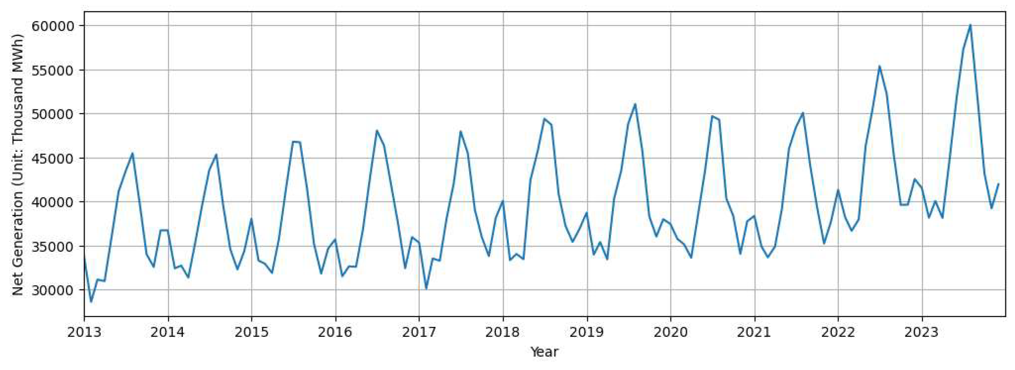
Figure 2.
Monthly Average Electricity Demand for Each Month (Unit: 1,000 MWh).
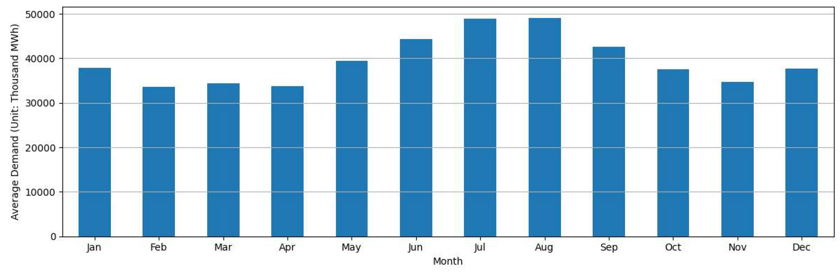
Figure 3.
Monthly Electricity Demand vs. Average Temperature in Texas across Years.
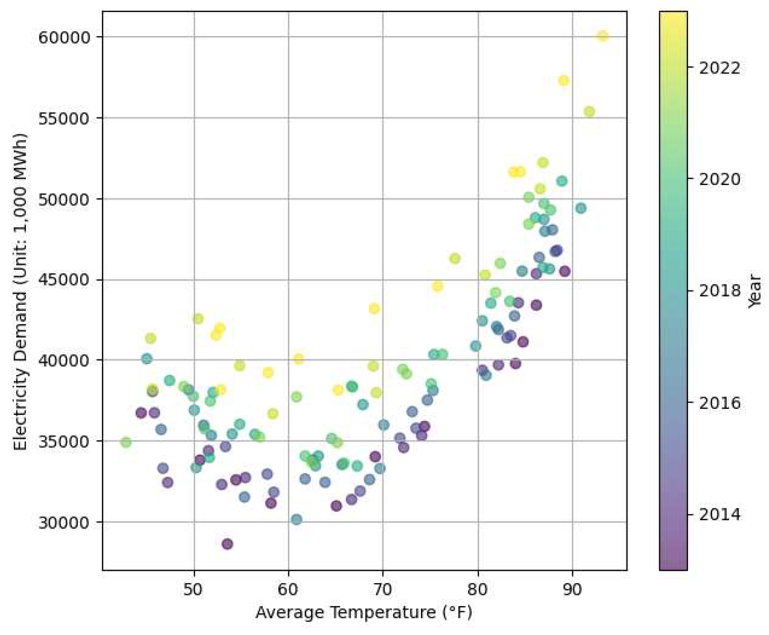
Figure 4.
Autocorrelation Function (ACF) Plot of Monthly Electricity Demand in Texas.
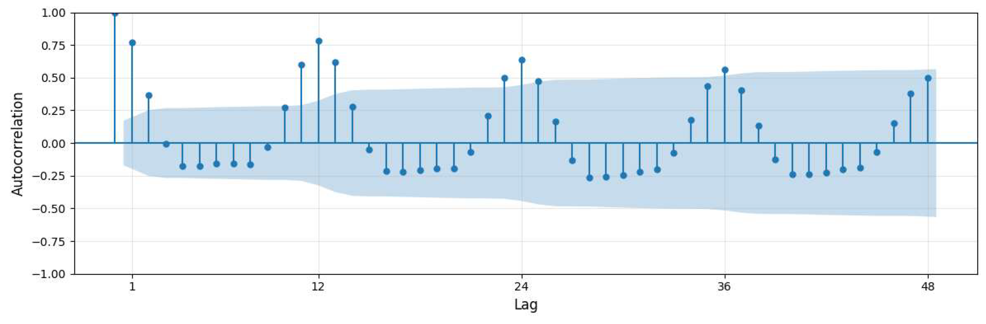
Figure 5.
Average Electricity Demand by (a) Number of Days in a Month and (b) Number of Weekday Holidays in a Month.
Figure 5.
Average Electricity Demand by (a) Number of Days in a Month and (b) Number of Weekday Holidays in a Month.
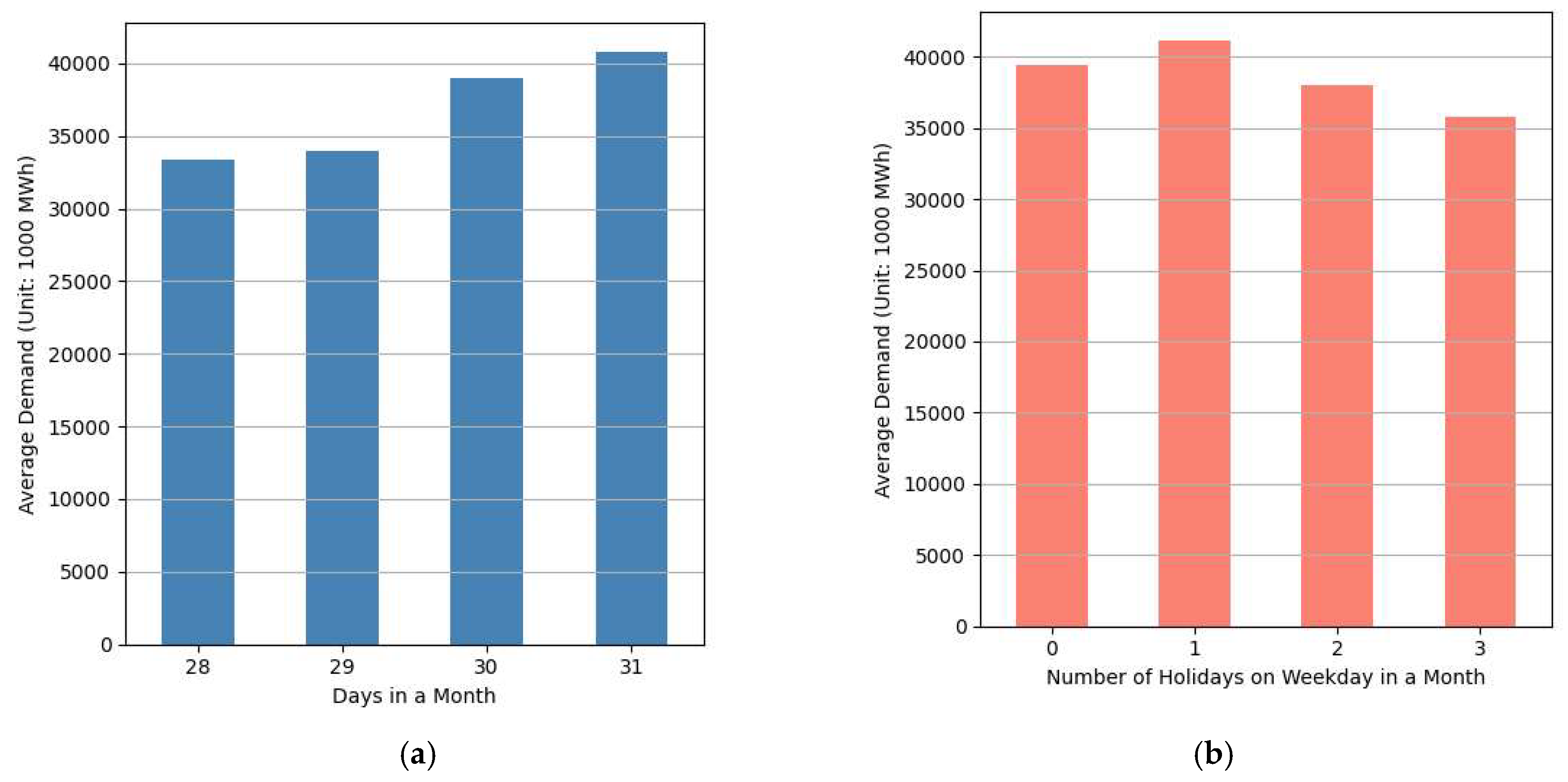
Figure 6.
Monthly Average Electricity Demand in Arranged in Ascending Order.
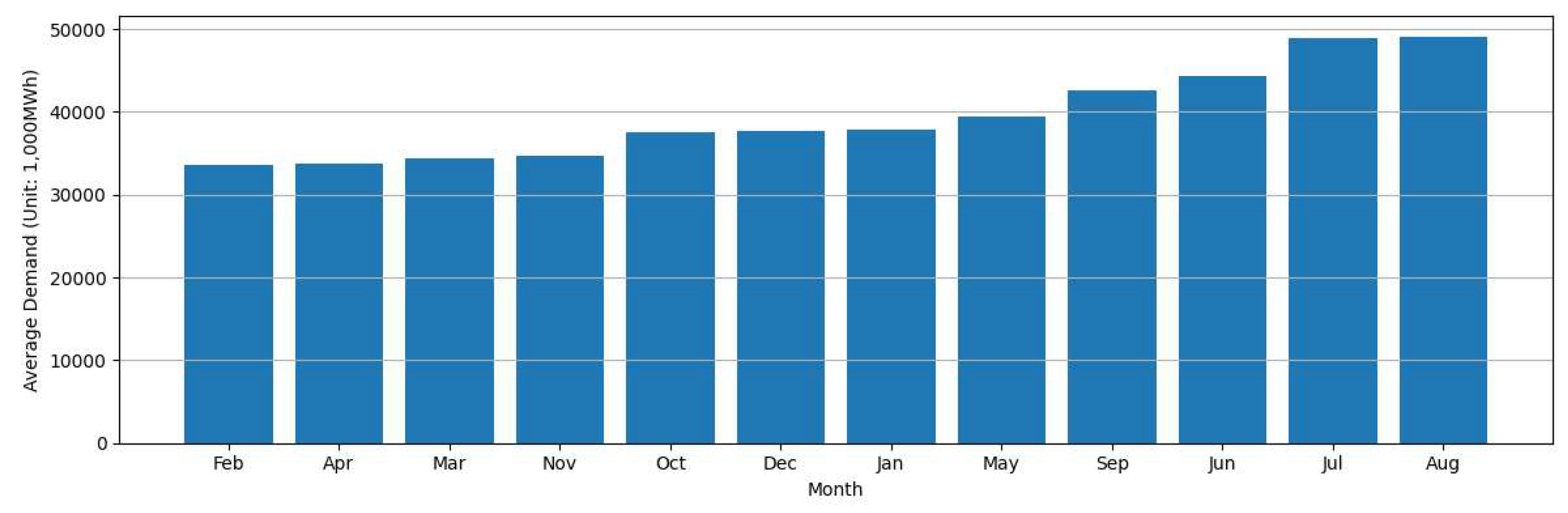
Figure 7.
Actual and Forecasted Monthly Electricity Demand in Texas for 2024 Across Different Methods.
Figure 7.
Actual and Forecasted Monthly Electricity Demand in Texas for 2024 Across Different Methods.
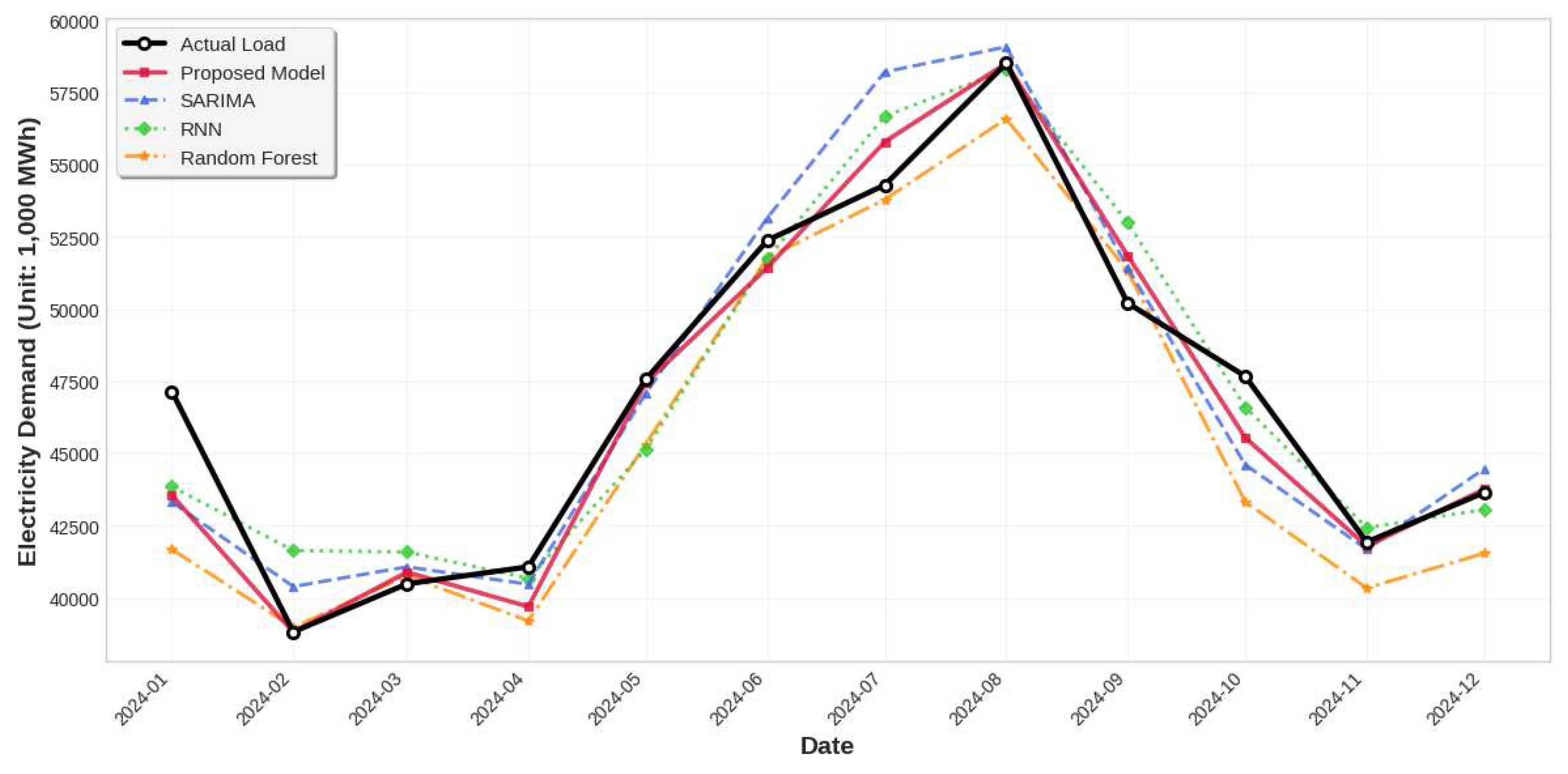

Table 1.
Summary of Load Forecasting Research for the Texas Region.
| Papers | Timeframes | Target Regions | Models Used | Key Features |
|---|---|---|---|---|
| Ali (2024) [13] | Hourly | Texas | RNN-LSTM-GRU | Past load and weather data |
| Derner et al. (2024) [14] | Daily | Texas | ARIMA and Linear Model | Past load, weather, calendar, and fuel type data. |
| Eysenbach et al. (2021) [15] | Daily | Texas | RNN-LSTM, ARUMA and VAR | Past load, weather, and population data |
| Hossain (2022) [16] | Hourly | West Texas | LSTM and GRU | Past load, weather data |
| Mostafa et al. (2024) [17] | Hourly | West Texas | RNN,LSTM and GRU | Past load, weather and calendar data |
| Rice et al. (2022) [18] | Hourly | Texas | Ridge and Lasso regressions | Past load and calendar data |
| Ruthford and Sadler (2021) [19] | Hourly | Texas | ARIMA and TSLM | Past load and weather data. |
| Singh (2024) [20] | Hourly | Texas | Generalized Additive Models | Past load and weather and calendar data. |
| Yang et al. (2024) [21] | Hourly | Texas | LSTM and FCNN | Past load, weather and calendar data |
Table 2.
Correlation Coefficient Values Between Monthly Electricity Demand and Average Monthly Temperature in Different Region in Texas.
Table 2.
Correlation Coefficient Values Between Monthly Electricity Demand and Average Monthly Temperature in Different Region in Texas.
| Cities | Dallas | Houston | Austin | San Antonio | Average |
|---|---|---|---|---|---|
| Correlation Coefficients | 0.715 | 0.707 | 0.714 | 0.702 | 0.711 |
Table 3.
Summary of Regression Coefficients.
| Variables | Coefficients | Standard Errors | t-statistics | p-values |
|---|---|---|---|---|
| Intercept | 112600 | 30100 | 3.738 | 0.000 |
| t2 | 0.2601 | 0.035 | 7.374 | 0.000 |
| yt−12 | 0.3291 | 0.095 | 3.464 | 0.001 |
| yt−13 | 0.0669 | 0.044 | 1.507 | 0.134 |
| mt | 891.6009 | 152.738 | 5.837 | 0.000 |
| Tt | -1487.7407 | 482.354 | -3.084 | 0.003 |
| dt | -3216.6054 | 955.935 | -3.365 | 0.001 |
| ℎt | -286.2095 | 223.68 | -1.28 | 0.203 |
| Tt⋅dt | 49.561 | 15.897 | 3.118 | 0.002 |
Table 4.
Results of Tested Methods.
| Methods | MAE | RMSE | MAPE | |
|---|---|---|---|---|
| Proposed Model | 999.5 | 1455.2 | 2.10% | |
| Benchmarks | Holt-Winters | 2340.5 | 2885.8 | 4.86% |
| SARIMA | 1475.3 | 1957.4 | 3.09% | |
| Prophet | 1606.4 | 1982.6 | 3.55% | |
| RNN | 1518.6 | 1864.2 | 3.28% | |
| LSTM | 3227.4 | 3801.9 | 6.89% | |
| Random Forest | 1851.2 | 2415.4 | 3.94% | |
| LightGBM | 2052.6 | 2468.8 | 4.24% | |
| XGBoost | 1904.9 | 2372.0 | 4.13% | |
Disclaimer/Publisher’s Note: The statements, opinions and data contained in all publications are solely those of the individual author(s) and contributor(s) and not of MDPI and/or the editor(s). MDPI and/or the editor(s) disclaim responsibility for any injury to people or property resulting from any ideas, methods, instructions or products referred to in the content. |
© 2025 by the authors. Licensee MDPI, Basel, Switzerland. This article is an open access article distributed under the terms and conditions of the Creative Commons Attribution (CC BY) license (http://creativecommons.org/licenses/by/4.0/).
Copyright: This open access article is published under a Creative Commons CC BY 4.0 license, which permit the free download, distribution, and reuse, provided that the author and preprint are cited in any reuse.


