Submitted:
20 January 2026
Posted:
21 January 2026
You are already at the latest version
Abstract
Remote sensing semantic segmentation encounters several challenges, including scale variation, the coexistence of class similarity and intra-class diversity, difficulties in modeling long-range dependencies, and shadow occlusions. Slender structures and complex boundaries present particular segmentation difficulties, especially in high-resolution imagery acquired by satellite and aerial cameras, UAV-borne optical sensors, and other imaging payloads. These sensing systems deliver large-area coverage with fine ground sampling distance, which magnifies domain shifts between different sensors and acquisition conditions. This work builds upon DeepLabV3+ and proposes complementary improvements at three stages: input, context, and decoder fusion. First, to mitigate the interference of complex and heterogeneous data distributions on network optimization, a feature-mapping network is introduced to project raw images into a simpler distribution before they are fed into the segmentation backbone. This approach facilitates training and enhances feature separability. Second, although the Atrous Spatial Pyramid Pooling (ASPP) aggregates multi-scale context, it remains insufficient for modeling long-range dependencies. Therefore, a routing-style global modeling module is incorporated after ASPP to strengthen global relation modeling and ensure cross-region semantic consistency. Third, considering that the fusion between shallow details and deep semantics in the decoder is limited and prone to boundary blurring, a fusion module is designed to facilitate deep interaction and joint learning through cross-layer feature alignment and coupling. The proposed model improves the mean Intersection over Union (mIoU) by 8.83% on the LoveDA dataset and by 6.72% on the ISPRS Potsdam dataset compared to the baseline. Qualitative results further demonstrate clearer boundaries and more stable region annotations, while the modifications to the baseline are minimal and easy to integrate into camera-based remote sensing pipelines and other imaging-sensor systems.
Keywords:
remote sensing
; semantic segmentation
; DeepLabV3+
; multi-level feature fusion
; global context modeling
1. Introduction
High-resolution remote sensing semantic segmentation presents significant challenges due to factors such as large-scale variation, intra-class diversity, and shadow occlusions. Elongated structures, narrow roads, rivers, and complex man-made boundaries pose particular difficulties in large orthorectified tiles characterized by heterogeneous land covers [1]. In practice, these tiles originate from a variety of optical sensors—including spaceborne and airborne frame cameras, push-broom scanners, and UAV-borne digital cameras—whose different viewing geometries, point-spread functions, and spectral responses further amplify intra-class variability and sensor-dependent artifacts. Recent work in Sensors has shown that even carefully designed networks such as LKAFFNet [2], MFPI-Net [3], and RST-Net [4] still struggle to balance multi-scale feature modeling and boundary sharpness on high-resolution land-cover scenes captured by such cameras. Furthermore, the combination of dense urban scenes and sparsely populated rural areas often results in severe class imbalance and domain shifts. Additionally, cast shadows and seasonal variations in illumination further compromise local contrast and edge fidelity. Collectively, these factors underscore the dual necessity for local detail preservation and long-range semantic consistency—requirements that are inherently challenging to fulfill simultaneously within latency-sensitive pipelines implemented in practical applications.
To improve global relation modeling within segmentation systems, a prominent line of work replaces convolutional encoders with hierarchical transformer designs or hybrid CNN and Transformer backbones. Wang et al. propose UNetFormer, an efficient UNet-style transformer that streamlines the decoder and sustains real-time segmentation on urban imagery [5]. Liu et al. design AMTNet with attention-based multiscale transformers in a CNN and Transformer Siamese framework to enhance multi-level context aggregation [6]. X. Liu et al. develop CSWin-UNet, integrating cross-shaped-window attention into a U-shaped architecture to better capture elongated patterns under controlled complexity [7]. Beyond backbones, Fan et al. introduce DDPM-SegFormer, which fuses diffusion features with a transformer to enhance land use and land cover delineation [8]; Chen et al. then propose CTFuse, a serial CNN to Transformer hybrid with spatial and channel attention that attains competitive results on ISPRS Potsdam and Vaihingen [9]. Despite these advances, many architectures deviate from the widely used CNN plus ASPP interface and can incur nontrivial memory and latency when operating on very large inputs typical in remote sensing workflows.
On the input side, researchers increasingly address photometric degradation and distribution shift prior to feature extraction. Lightweight restoration tailored to remote sensing imagery-such as axial depthwise convolutions coupled with hybrid attention-improves visibility under haze and occlusions at modest cost [10]. Complementary frequency-space approaches align amplitude statistics or leverage wavelet-guided adaptation to correct distribution mismatch at the source, improving cross-domain robustness without heavy architectural changes [11,12]. In parallel, dynamic and sparse strategies prune or select tokens or regions to contain the cost of global modeling while retaining long-range dependencies. For instance, recent work on dynamic token pruning for semantic segmentation proposes a method that grades token difficulty and allows easy tokens to exit early. This approach significantly reduces computational cost by approximately 20% to 35% with minimal loss of accuracy [13]. In addition to single-modal enhancements, multimodal fusion networks that jointly process optical camera imagery and auxiliary height-related sensors have demonstrated improved robustness to shadows and sensor-specific artefacts, as illustrated by recent Mamba-based multimodal architectures such as MMFNet [14].
For the decoder and boundary-refinement stage, in-network mechanisms originally developed for generic semantic segmentation continue to offer improvements in thin-structure continuity and edge fidelity. For example, BASeg employs a boundary-refined module combined with context aggregation to enhance object boundaries and fine structures, especially in scenes with complex shapes and multiple small or adjacent objects [15]. Edge-aware multi-task learning jointly predicts masks, edges, and distance maps to regularize boundaries and close small parcels [16]. Context-feature-enhanced decoders further strengthen region-level discrimination and stabilize fine categories in complex scenes. For instance, FBRNet incorporates a border-refinement module together with feature-fusion and multi-scale context aggregation to better preserve fine structures and sharp boundaries in challenging segmentation scenarios [17]. Nevertheless, many refinements still rely on heavy multi-branch decoders or specialized heads that complicate engineering migrations and may not map cleanly onto standard CNN plus ASPP toolchains.
To address these issues while preserving the DeepLabV3+ pipeline, we propose LGD-DeepLabV3+ with three plug-in modules:
(1) Laplacian-guided Input Shaping (LIS). Multi-level Laplacian decomposition followed by lightweight nonlinear remapping reshapes the input distribution, suppresses cross-frequency interference, and improves early feature separability with negligible overhead, while keeping the encoder interface unchanged.
(2) Global Context Routing (GCR) after ASPP. A routing-style global modeling block at the ASPP output (one-sixteenth scale) performs coarse region scoring to select top- candidates, then computes fine attention only within their union, yielding near-global dependencies and cross-region consistency at low compute and memory cost, without modifying the backbone or the training recipe.
(3) Directional Perception Fusion (DPF) in the decoder. After shallow and deep feature concatenation, coordinate-aware spatial recalibration, local refinement, and cross-layer channel coupling enhance elongated structures and true boundaries while suppressing texture-induced false positives, all within a lightweight decoder interface.
2. Methods
2.1. Overall Framework of LGD-DeeplabV3+
This paper takes the encoder-decoder paradigm of DeepLabV3+ as the baseline [18]. The input image is first processed by the convolutional backbone to extract features, and the ASPP at the top layer performs multi-scale context aggregation. The decoder retrieves details from earlier layers and concatenates them with the upsampled semantic layers, ultimately producing pixel-level predictions. Without changing the main structure or tensor interfaces, we insert lightweight and pluggable enhancement modules at three key locations, forming LGD-DeepLabV3+, as shown in Figure 1. Because all three modules are implemented as generic convolution and attention operators that act on image tensors, they are agnostic to the underlying imaging sensor and can in principle be applied to RGB/IRRG aerial cameras, multispectral satellite sensors, and multimodal image–DSM pairs without modifying the backbone interface. These three locations are: the input side before the backbone, the context stage after ASPP, and after the shallow-deep feature concatenation in the decoder.
The input side is handled by the LISModule, which performs feature re-shaping using Laplacian-pyramid decomposition to obtain high-frequency details and low-frequency residuals, preserving fine structures and global context. This method has been effective in segmentation tasks [19]. These components are then reshaped non-linearly and compressed in channels using lightweight KAN convolutions, while maintaining the spatial resolution. The features at each scale are upsampled to a consistent size and later fused laterally to produce reshaped features of the same size as the input. This process, implemented before entering the backbone, achieves weak decoupling and distribution reshaping, allowing high-frequency textures to be preserved without excessive magnification, while low-frequency structures are calibrated to a more regular statistical state. As a result, it provides a more optimized starting point for subsequent feature learning and maintains consistency with the input channels and data format of the backbone.
After the ASPP, the GCRModule is introduced to reinforce long-range dependencies and global consistency. This module adopts a two-stage routing strategy that first performs coarse selection and then fine-grained computation. In the coarse-grained stage, the feature map from ASPP is divided into a regular grid, and candidate region scores are generated for each query position. Only the top-scoring candidates are retained to form the attention range. The fine-grained stage then executes multi-head attention and linear transformations within the union of these candidate regions, completing information exchange. This is followed by residual connections and normalization to stabilize training, and the output is mapped back to the required number of channels in the backbone using a 1×1 convolution. The demand-driven routing ensures that each position connects only with a few relevant areas, maintaining near-global perception while keeping computational and memory costs within acceptable limits [20]. As the working resolution is consistent with ASPP, the multi-scale features from GCRModule and ASPP complement each other without requiring changes to the backbone or tensor sizes.
In the decoding stage, the DPFModule performs direction-sensitive recalibration, local refinement, and cross-layer channel interactions. After shallow details and deep semantics are concatenated at the same resolution, spatial recalibration is performed through coordinate decomposition, followed by 1D global pooling along the row and column directions to obtain two context clues sensitive to direction. These shallow and deep branches form four attention branches-shallow row, shallow column, deep row, and deep column-to generate fine-grained spatial guidance maps, performing direction-sensitive recalibration on the concatenated features. Building on this, two layers of 3×3 convolutions are stacked, or layer-wise depth-wise convolutions are used to achieve lightweight processing, emphasizing real boundaries while suppressing false responses caused by textures. Shallow and deep channels are then globally pooled separately to form compact channel representations, which are linearly mapped to obtain mutually gated channel weights, allowing shallow details and deep semantics to align cooperatively along the channel dimension. The DPFModule prioritizes maintaining boundaries and slender structures, significantly improving the stability of shallow-deep fusion with minimal increases in parameters and computational cost. The module’s output is then directly connected to the 3×3 convolution and upsampling path of DeepLabV3+, maintaining interface consistency.
The three modules together form LGD-DeepLabV3+. The input reshaping stabilizes the data distribution and reduces optimization difficulty, while the routing-based global modeling in the context stage captures cross-region relationships more efficiently. The direction-sensitive fusion in the decoder strengthens the delineation of real boundaries and small targets. The entire solution preserves the end-to-end training flow and is easy to integrate and migrate into existing systems, while being more computationally and memory-efficient [21].We next detail each component and the training objectives.
2.2. LISModule
To reduce optimization difficulty before entering the backbone and ensure both large-area consistency and boundary distinguishability, the input side adopts a pre-processing strategy of four-level Laplacian decomposition followed by layer-wise KAN convolutions. First, the image is decomposed into multi-frequency components using a four-level Laplacian pyramid [22]. Then, multi-scale information is fused at the original resolution. Finally, KAN convolution is applied for lightweight shaping and channel alignment, and the resulting features are passed to the DeepLabV3+ backbone. This is the overall process of Laplacian-guided Input Shaping (LIS) Module, as shown in Figure 2.
The input image is first processed by a four-level Laplacian pyramid to complete frequency decomposition and separation, The input image is first decomposed into multiple frequency bands by a four-level Laplacian pyramid. Let represent the -th high-pass filter in the pyramid. The filter used has a kernel of h = [1,4,6,4,1]/16, with a 5×5 size, and is calculated by:
The corresponding Laplacian components are defined by:
For each component at each scale, a KAN convolution operator, denoted as KANConv [23], is introduced. It approximates nonlinear mapping and performs channel compression using learnable basis functions within a fixed local neighborhood. Let the receptive field size k be 3, and the number of basis functions M be 6. Then, for any position p and output channel o, is given by:
Here, represents the k×k neighborhood, and are the fixed B-spline bases, with and being learnable coefficients. Let the output of this scale be denoted as , and then are progressively upsampled to the original resolution and later fused horizontally to form intermediate features. Let denote the feature obtained by upsampling ell from scale to the reference resolution. This is given by:
The term represents upsampling to the same resolution as the input by a factor of , where denotes the use of Batch Normalization (BN) and GELU. To match the main interface, the final 1×1 convolution maps the channels to the expected input channels, while keeping the spatial size unchanged.
2.3. GCRModule
To further model long-range dependencies while maintaining low computational overhead after ASPP, this paper inserts a Global Context Routing (GCR) Module at the 1/16 scale. The core idea is to first perform coarse filtering followed by fine-grained calculations. Initially, candidate routing is selected at the region level, and then fine-grained attention is applied only to the union of these candidates. This allows each position to interact with only a small number of relevant regions, thereby approximating global perception while significantly reducing irrelevant computations [24]. The process is shown in Figure 3.
Let the output of ASPP be (where , are the height and width of the original image, respectively, and the scale is 1/16). The feature map is divided into a non-overlapping grid of ×, and the region index .The key, value, and other computations are derived from:
Each region-level grid is averaged to obtain the region-level representation ,, where is the grid size and is the number of channels. The region similarity is computed, and for each query region, the top- most relevant regions are selected from a row of , obtaining the selection set . Then, the detailed computation on the selected set is performed, where the corresponding keys and values are collected based on , forming the compact candidate union . The attention points are summed up and projected back into the original channel. Meanwhile, 3×3 depthwise convolutions are applied to enhance spatial locality, suppress noise, and strengthen the boundaries. The model uses Pre-Norm residuals and trains with a two-layer MLP, as described in:
The routing attention interaction is given by:
The channel reconstruction output is given by:
The MLP consists of two linear layers with GELU activation and a default expansion ratio of 4. When necessary, a 1×1 linear layer is used to align the channel dimension We set the grid size , the number of routed candidates , and the number of attention heads to 8, which complements the multi-scale context of ASPP without changing the resolution. Finally, is upsampled by a factor of 4 to and fused with the shallow decoder features at the same scale, as shown in Figure 4.
Figure 4 shows the structure of the GCRModule Block. This block forms a local multi-scale interaction with the ASPP, serving as a global supplement before the decoder. In the routing stage, the × grid regions are formed based on the area similarity, and top- related regions are selected. The feature map is further enhanced with a 3×3 depth convolution and MLP, ensuring stability and good linear continuity. The final output, is then fused with the decoder’s shallow features at the same resolution.
2.4. DPFModule
The decoder combines the high-level features with low-level fine-grained features through concatenation at the same spatial resolution . At the same time, it enhances the global and local context sensitivity, as well as edge refinement and channel selection. After the concatenation, the fine-grained fusion module, Directional Perception Fusion(DPF) Module, is introduced. It adjusts the attention direction to align with the local refinement and then passes through the sequential aggregation [25]. This helps to suppress the noise and improve the continuity of fine structures. To facilitate the integration with the later model, a 1×1 convolution is first used to align the channels to , as shown in Figure 5.
First, perform 1D global pooling along the row and column directions to obtain statistical values in both directions, as shown:
Initially, concatenate along the length dimension and pass it through a shared 1×1 convolution to obtain the intermediate representation. Then, split the direction into two branches, producing the attention maps and for the vertical and horizontal directions, respectively. The elements are then summed along the dimension, and the spatial weight is computed, where indicates element-wise multiplication. The stabilization of the enhanced features is detailed in:
Two layers of 3×3 convolution are added to , with each layer followed by normalization and ReLU activation. The residual branch is maintained, which helps to suppress the unwanted responses generated by enhanced edge features. This process is denoted as , as expressed in:
Subsequently, the concatenation is normalized without altering the spatial distribution, and multi-branch concatenation and re-normalization are performed for . First, a global average pooling is applied to obtain a description of the feature map, . Then, branches are used, and each branch applies two layers of sensory detectors to perform a non-linear transformation of [26], which is defined for the b-th branch as:
Notably, refers to the reduction in dimensions. Here, represents the ReLU function, which outputs the concatenated feature vector along the channel dimension ,followed by a linear transformation. The concatenated output is then mapped to the channel dimension and passed through the attention weights as shown:
Here represents the sigmoid function to implement a gating mechanism. Finally, the output is normalized through the attention mechanism to obtain the Directional Perception Fusion (DPF) output, as shown:
The default setting for the number of branches and compression rate is both 4. This design allows for the simultaneous activation of multiple channels, making it more suitable for multi-class fine-grained representation. Additionally, the entire DPF branch maintains consistency with the decoder interface in both spatial scale and tensor shape.
2.5. Loss Function and Training Objective
The study conducts supervision on the LoveDA and ISPRS Potsdam datasets with a step length of 4, using a combination of cross-entropy (CE) and multi-class Dice loss to balance class accuracy and the recall of uneven regions. The output class logits from the classifier are denoted as , and the class probabilities , are calculated using the softmax function, where for the range of classes, and 255 represents invalid pixels. The mask M is defined as 1 indicating the valid pixel area. The classification loss is computed by:
Let denote the one-hot label for the k-th class; we define the corresponding Dice coefficient and the macro-averaged multi-class Dice loss as follows:
The final objective is a weighted sum of cross-entropy and macro-averaged Dice losses that balances calibration and overlap quality, with ; it is computed only on valid pixels, as follows:
The cross-entropy focuses on the consistency of the pixel-level class and the accuracy of classification; Dice focuses on balancing class distribution, fine-grained structures, and sparsity. Under the goal of improving regional consistency and recall, the above loss avoids position calculation when = 1, avoiding optimization of ineffective areas in the data or its own sparse regions. An is used to stabilize the values. In cases where there is complete class deficiency in certain classes in the dataset, the average per class can be selected to appear only in certain cases without affecting the conclusions.
2.6. Experimental Setup
The computational hardware used in this study consisted of a workstation running Ubuntu 24.04.3 LTS and four NVIDIA GeForce RTX 3090 GPUs, each with 24 GB of memory. The software environment comprised Python 3.8 (Conda), PyTorch 1.10.0, torchvision 0.11.1, and MMCV-Full 1.7.0 built for CUDA 11.3 and PyTorch 1.10. Additional libraries included TensorBoard 2.11.0, timm, segmentation-models-pytorch, OpenCV-Python, einops, scikit-image, PyWavelets, pytorch_wavelets, and pytorch_msssim. We trained the model for 50,000 iterations with a per-GPU batch size of 4, using Adam with beta1 = 0.9 and beta2 = 0.999. The initial learning rate was 1e-3 and the weight decay was 5e-3; the learning rate followed a polynomial decay schedule with power 0.9 and a minimum of 1e-5. For LoveDA, images were resized to 1024×1024 and randomly cropped to 512×512; for ISPRS Potsdam, we used pre-sliced 512×512 patches. We applied only photometric augmentations-color and brightness and standard intensity normalization, while geometric transforms were disabled to keep comparisons controlled. At inference, we used single-scale sliding-window evaluation with a 512×512 window and a 256 stride, averaging predictions over overlaps to obtain the final segmentation at the original image resolution. Pixels labeled 255 were treated as invalid and ignored during loss computation and metric evaluation. Key training parameters are summarized in Table 1.
3. Experiment
3.1. Dataset and Evaluation Protocol
3.1.1. Loveda Dataset
LoveDA is an urban-rural dual-domain semantic segmentation dataset with RGB tiles collected from cities including Nanjing, Changzhou, and Wuhan [27]. Each tile has a ground sampling distance of approximately 0.3 m and a size of 1024×1024 pixels. The imagery is acquired by high-resolution optical cameras sensor on airborne or satellite platforms; in this work, we follow the common setting that uses only the three visible bands, treating the dataset as representative of camera-based land-cover mapping in operational remote sensing systems. The official split contains 2,522 training images, 1,669 validation images, and 1,796 test images. The label set comprises seven categories: background, building, road, water, barren, forest, and agriculture. LoveDA spans dense urban scenes and sparsely populated rural environments with substantial scale variation and class imbalance, making it a widely used benchmark for assessing cross-domain robustness and boundary delineation. Figure 6 shows representative LoveDA RGB tiles and their pixel-level annotations for the seven classes. The preprocessing and evaluation protocols for LoveDA follow Section 2.3.
3.1.2. ISPRS Potsdam Dataset
The ISPRS Potsdam dataset contains orthorectified aerial images from urban areas. Each full tile has a typical size of 6000×6000 pixels and a ground sampling distance of 5 cm [28]. We use the IRRG three-channel imagery composed of near-infrared, red, and green bands. These tiles are captured by a very high-resolution digital aerial camera, and the inclusion of a near-infrared band makes the dataset representative of multi-band optical sensors widely used for urban monitoring. The dataset includes six categories: impervious surface, building, low vegetation, tree, car, and clutter/background. It covers common urban elements such as road networks, rooftops, and trees, which makes it suitable for assessing fine-grained segmentation and boundary delineation under high-resolution conditions. Figure 7 shows representative IRRG tiles and their pixel-level annotations for the six classes. For reproducibility, we adopt a fixed split with 30 full images for training and 7 for validation; the same seven images are used for testing. The 6000×6000 tiles are grid-sliced offline into 512×512 patches and these patches are used directly for training. All remaining preprocessing and evaluation protocols follow Section 2.3.
3.1.3. Evaluation Setup and Metrics
The evaluation is conducted using a single-scale sliding window, with the entire image predicted using a 512×512 window and a stride of 256. The category probabilities of the overlapping regions are averaged and fused to obtain segmentation results with the same dimensions as the original image. Unless otherwise specified, no multi-scale or mirroring augmentations are applied during testing. All metrics are calculated only on valid labeled pixels.
Based on the definition of the metrics, for class c, the confusion counts are True Positive (), False Positive (), and False Negative (). The IoU for class c is calculated using the formula shown:
The precision and recall for class c are are represented by:
The pixel-level score is equivalent to the Dice coefficient, so the values of and in the following tables are the same. We report absolute gains in percentage points, denoted as pp. The macro-average and are given by:
Let be the × pixel-level confusion matrix, then the overall accuracy (OA) is given by:
3.2. Comprehensive Comparison Experiments on the LoveDA Dataset
LoveDA covers both urban and rural domains and has an imbalanced class distribution, making it suitable for testing cross-domain robustness and multi-scale modeling capabilities. In a unified setup comparing BiSeNetV2 [29], PSPNet [30], ResUNet [31], SegFormer [32], and Swin-Tiny [33], etc., we compare the baseline DeepLabV3+ with the comprehensive improvement LGD-DeepLabV3+(LISModule + GCRModule + DPFModule). The overall results are shown in Table 2.
Compared to the baseline, LGD-DeepLabV3+ achieves consistent improvements on LoveDA, with mIoU increasing from 49.65% to 58.48%, a gain of 8.83%; F1 improving from 65.48% to 73.37%, a gain of 7.89%; and OA rising from 71.39% to 76.32%, a gain of 4.93%. Compared to other representative methods, LGD-DeepLabV3+ leads overall in mIoU and F1, indicating that the input-side shaping LISModule, the global context routing GCRModule after ASPP, and the decoder-side detail fusion DPFModule work together to provide complementary gains in cross-domain scenarios. Class-wise comparisons are shown in Table 3.
The improvement is particularly significant in slender or weak-texture categories. The IoU for barren increased by 17.87%, and F1 by 19.77%; the IoU for road increased by 11.28%, and F1 by 9.86%; the IoU for water increased by 9.95%, and F1 by 7.09%; agriculture and building also improved by 8.01% and 6.80%, respectively. Consistent qualitative effects are evident in Figure 8, where LGD-DeepLabV3+ yields more continuous thin roads and rivers, clearer building boundaries under shadows, and fewer barren–water confusions than the baselines.
3.3. Comprehensive Comparison Experiments on the ISPRS Potsdam Dataset
ISPRS Potsdam has a 5 cm resolution with rich small targets and clear boundaries, making it suitable for testing the overall capability of long-range modeling and boundary delineation. The evaluation protocol and comparison methods from Section 3.2 are followed, with the overall results shown in Table 4.
Compared to the DeepLabV3+ baseline, LGD-DeepLabV3+ achieves comprehensive improvements on ISPRS Potsdam, with mIoU increasing from 74.07% to 80.79%, a gain of 6.72%; F1 improving from 84.60% to 89.16%, a gain of 4.56%; and OA rising from 86.72% to 90.34%, a gain of 3.62%. Compared to other representative methods, LGD-DeepLabV3+ leads overall in mIoU and F1, validating the effectiveness of the proposed modules in high-resolution urban scenes. Class-wise comparisons are shown in Table 5.
As seen in Table 5, all classes show improvements. Specifically, the IoU for background increased by 16.57%, and F1 by 12.59%; the IoU for impervious surfaces improved by 5.78%, and F1 by 3.36%; the IoU for low vegetation and tree both improved by 5.22%, with F1 increasing by 3.45% and 3.54%, respectively; car and building also achieved IoU increases of 4.03% and 3.52%, with F1 improving by 2.51% and 1.92%, respectively. This indicates that the LISModule on the input side helps reshape the distribution of weak-texture regions, the GCRModule after ASPP enhances long-range consistency across regions, and the DPFModule at the decoder side suppresses false textures and improves boundary quality in shallow-deep fusion. The synergy of these three modules brings stable gains. Qualitative results are shown in Figure 9.
3.4. Ablation Study and Complexity Trade-Off
Under the same data processing and training protocol, using DeepLabV3+ as the baseline, we sequentially insert individual enhancement modules or concatenate all three. Specifically, +LISModule indicates the pre-shaping with Laplacian pyramid + KAN convolutions at the input side; +GCRModule refers to adding global context routing after ASPP; +DPFModule represents direction recalibration at the shallow-deep concatenation stage, followed by two 3×3 convolutions and channel aggregation; LGD-DeepLabV3+ represents the concatenation of all three modules in the order shown in Figure 3, Figure 4 and Figure 5. The remaining training and inference settings are consistent with the baseline. The evaluation uniformly reports OA, mIoU, and F1, along with the percentage improvement Δ relative to the baseline. Table 6 presents the ablation comparison on LoveDA.
As shown in Table 6, all three modules bring stable gains on the LoveDA dataset. After adding the LISModule, the improved input distribution leads to more stable recognition of weak-texture and complex background regions, with significant improvements in both mIoU and F1. After adding the GCRModule, long-range consistency is significantly enhanced without changing the resolution, with the most significant improvements seen in connected structures such as roads and rivers. After adding the DPFModule, boundaries and slender targets become clearer, with the largest improvement in F1. In LGD-DeepLabV3+, the complementary effects of the three modules result in the best performance, with mIoU increasing by +8.83pp, F1 by +7.89pp, and OA by +4.93pp. Table 7 presents the ablation comparison on ISPRS Potsdam.
Due to the higher resolution and clearer boundaries, the benefits of the GCRModule are most pronounced; LGD-DeepLabV3+ achieves the highest scores across all three metrics. The GCRModule primarily drives the improvement in mIoU, the LISModule provides stable robustness gains in complex textured backgrounds, and the DPFModule further refines boundaries and small targets. This indicates that in high-resolution urban scenarios, cross-region dependencies and global consistency are more critical. The synergy of LGD-DeepLabV3+ is evident, with mIoU improving by +6.72pp, mF1 by +5.01pp, and OA by +3.62 pp relative to the baseline.
The complexity and efficiency statistics are shown in Table 8, all obtained under a unified inference setup. The baseline has the lightest computation and the lowest latency; when only the GCRModule is added, the parameter and memory overhead are moderate, providing stable improvements in mIoU and mF1 without changing the resolution or interface, making it suitable for latency-sensitive scenarios. After the three modules are concatenated to form LGD-DeepLabV3+, the computational and memory costs increase significantly, but the best and most balanced accuracy improvements across datasets are achieved, with notable improvements in long-range consistency, slender structures, and real boundary delineation. Overall, while the single modules provide low-cost, plug-and-play gains, the complete framework achieves the best accuracy within acceptable overhead.
4. Conclusions
This paper proposes LGD-DeepLabV3+ based on the DeepLabV3+ baseline, forming a collaborative framework with three pluggable enhancements that span input shaping, global modeling, and decoding refinement. The input-side LISModule reshapes the distribution and stabilizes optimization through Laplacian decomposition and lightweight KAN convolutions. The GCRModule, placed after ASPP, applies routing-based global modeling, focusing computation on relevant regions to strengthen long-range dependencies and cross-region consistency. The DPFModule at the decoder end enhances boundary and slender target delineation through direction recalibration, local refinement, and channel aggregation. Under a unified training and evaluation setup, the method achieves an 8.83% increase in mIoU and a 7.89% increase in mF1 on LoveDA, and a 6.72% increase in mIoU and a 4.56% increase in mF1 on ISPRS Potsdam, with OA also improving. Road and water network continuity is stronger, and building and shadow boundaries are clearer. Each of the three modules provides independent gains, with the cascade achieving more balanced improvements in mIoU and mF1. The method can still maintain around 37.5 FPS during inference with a 512×512 input and batch size of 1, making it suitable for engineering integration and migration. The main bottlenecks currently lie in computational cost and cross-domain generalization. Future work will focus on lightweight and adaptive solutions, including pruning and quantization, knowledge distillation, dynamic routing and early stopping, domain adaptation, and multi-modal fusion, to further improve real-time performance and robustness in more complex and large-scale real-world scenarios. From a sensing perspective, LGD-DeepLabV3+ is agnostic to the specific camera or imaging sensor and operates directly on generic raster inputs. This makes it compatible with RGB/IRRG aerial cameras, multispectral satellite sensors, and multimodal image–DSM pairs similar to those used in recent Sensors architectures such as LKAFFNet, MFPI-Net, RST-Net, and MMFNet. In future work, we plan to explicitly validate the framework on additional sensor modalities, including UAV video cameras, SAR–optical fusion, and LiDAR-derived height maps, further tightening the connection between advanced sensing hardware and semantic segmentation algorithms.
Author Contributions
Conceptualization, X.W. and X.L. (Xu Liu); methodology, X.W. and X.L. (Xu Liu); software, A.M. and Y.Y; validation, Y.Y. and X.L. (Xipeng Li); formal analysis, X.L. (Xu Liu) and A.M.; investigation, Y.Y. and X.L. (Xipeng Li); resources, X.W.; data curation, X.W.; writing—original draft preparation, X.L. (Xu Liu); writing—review and editing, X.W. and X.L. (Xu Liu); visualization, A.M.; supervision, X.W. and X.L. (Xu Liu); project administration, X.W.; funding acquisition, X.W. and X.L. (Xu Liu). All authors have read and agreed to the published version of the manuscript.
Funding
This work was supported by the Science and Technology Development Plan Project of Jilin Province,China (Grant No. 20230101175JC).
Data Availability Statement
The original contributions presented in the research are included in the article, further inquiries can be directed to the corresponding author.
Conflicts of Interest
The authors declare no conflicts of interest.
References
- Li, J.; Cai, Y.; Li, Q.; Kou, M.; Zhang, T. A review of remote sensing image segmentation by deep learning methods. International Journal of Digital Earth 2024, 17, 2328827. [Google Scholar] [CrossRef]
- Chen, B.; Tong, A.; Wang, Y.; Zhang, J.; Yang, X.; Im, S.-K.J.S. LKAFFNet: A Novel Large-Kernel Attention Feature Fusion Network for Land Cover Segmentation. 2024, 25, 54. [Google Scholar] [CrossRef] [PubMed]
- Song, X.; Chen, M.; Rao, J.; Luo, Y.; Lin, Z.; Zhang, X.; Li, S.; Hu, X.J.S. MFPI-Net: A Multi-Scale Feature Perception and Interaction Network for Semantic Segmentation of Urban Remote Sensing Images. 2025, 25, 4660. [Google Scholar] [CrossRef]
- Yang, N.; Tian, C.; Gu, X.; Zhang, Y.; Li, X.; Zhang, F.J.S. RST-Net: A Semantic Segmentation Network for Remote Sensing Images Based on a Dual-Branch Encoder Structure. 2025, 25, 5531. [Google Scholar] [CrossRef]
- Wang, L.; Li, R.; Zhang, C.; Fang, S.; Duan, C.; Meng, X.; Atkinson, P.M. UNetFormer: A UNet-like transformer for efficient semantic segmentation of remote sensing urban scene imagery. ISPRS Journal of Photogrammetry and Remote Sensing 2022, 190, 196–214. [Google Scholar] [CrossRef]
- Liu, W.; Lin, Y.; Liu, W.; Yu, Y.; Li, J. An attention-based multiscale transformer network for remote sensing image change detection. ISPRS Journal of Photogrammetry and Remote Sensing 2023, 202, 599–609. [Google Scholar] [CrossRef]
- Liu, X.; Gao, P.; Yu, T.; Wang, F.; Yuan, R.-Y. CSWin-UNet: Transformer UNet with cross-shaped windows for medical image segmentation. Information Fusion 2025, 113, 102634. [Google Scholar] [CrossRef]
- Fan, J.; Shi, Z.; Ren, Z.; Zhou, Y.; Ji, M. DDPM-SegFormer: Highly refined feature land use and land cover segmentation with a fused denoising diffusion probabilistic model and transformer. International Journal of Applied Earth Observation and Geoinformation 2024, 133, 104093. [Google Scholar] [CrossRef]
- Chen, X.; Li, D.; Liu, M.; Jia, J. CNN and transformer fusion for remote sensing image semantic segmentation. Remote Sensing 2023, 15, 4455. [Google Scholar] [CrossRef]
- He, Y.; Li, C.; Li, X.; Bai, T. A Lightweight CNN Based on Axial Depthwise Convolution and Hybrid Attention for Remote Sensing Image Dehazing. Remote Sensing 2024, 16, 2822. [Google Scholar] [CrossRef]
- Ma, X.; Zhang, X.; Ding, X.; Pun, M.-O.; Ma, S. Decomposition-based unsupervised domain adaptation for remote sensing image semantic segmentation. IEEE Transactions on Geoscience and Remote Sensing, 2024. [Google Scholar]
- Xu, Q.; Zhang, R.; Fan, Z.; Wang, Y.; Wu, Y.-Y.; Zhang, Y. Fourier-based augmentation with applications to domain generalization. Pattern Recognition 2023, 139, 109474. [Google Scholar] [CrossRef]
- Tang, Q.; Zhang, B.; Liu, J.; Liu, F.; Liu, Y. Dynamic token pruning in plain vision transformers for semantic segmentation. In Proceedings of the Proceedings of the IEEE/CVF International Conference on Computer Vision, 2023; pp. 777–786. [Google Scholar]
- Qiu, J.; Chang, W.; Ren, W.; Hou, S.; Yang, R.J.S. MMFNet: A Mamba-Based Multimodal Fusion Network for Remote Sensing Image Semantic Segmentation. 2025, 25, 6225. [Google Scholar]
- Xiao, X.; Zhao, Y.; Zhang, F.; Luo, B.; Yu, L.; Chen, B.; Yang, C.J.N.N. BASeg: Boundary aware semantic segmentation for autonomous driving. 2023, 157, 460–470. [Google Scholar] [CrossRef]
- Li, M.; Long, J.; Stein, A.; Wang, X. Using a semantic edge-aware multi-task neural network to delineate agricultural parcels from remote sensing images. ISPRS journal of photogrammetry and remote sensing 2023, 200, 24–40. [Google Scholar]
- Qu, S.; Wang, Z.; Wu, J.; Feng, Y.J.P.A.; Applications. FBRNet: a feature fusion and border refinement network for real-time semantic segmentation. 2024, 27, 2. [Google Scholar] [CrossRef]
- Chen, L.-C.; Zhu, Y.; Papandreou, G.; Schroff, F.; Adam, H. Encoder-decoder with atrous separable convolution for semantic image segmentation. In Proceedings of the Proceedings of the European conference on computer vision (ECCV), 2018; pp. 801–818. [Google Scholar]
- Chen, Y.J.N.P.L. Semantic image segmentation with feature fusion based on Laplacian pyramid. 2022, 54, 4153–4170. [Google Scholar]
- Tong, L.; Li, W.; Yang, Q.; Chen, L.; Chen, P. Vision Transformer with Key-Select Routing Attention for Single Image Dehazing. IEICE TRANSACTIONS on Information and Systems 2024, 107, 1472–1475. [Google Scholar] [CrossRef]
- Cheng, H.; Wu, H.; Zheng, J.; Qi, K.; Liu, W. A hierarchical self-attention augmented Laplacian pyramid expanding network for change detection in high-resolution remote sensing images. ISPRS Journal of Photogrammetry and Remote Sensing 2021, 182, 52–66. [Google Scholar] [CrossRef]
- Yin, X.; Yu, Z.; Fei, Z.; Lv, W.; Gao, X. Pe-yolo: Pyramid enhancement network for dark object detection. In Proceedings of the International conference on artificial neural networks, 2023; pp. 163–174. [Google Scholar]
- Bodner, A.D.; Tepsich, A.S.; Spolski, J.N.; Pourteau, S. Convolutional kolmogorov-arnold networks. arXiv 2024, arXiv:2406.13155. [Google Scholar]
- Zhu, L.; Wang, X.; Ke, Z.; Zhang, W.; Lau, R.W. Biformer: Vision transformer with bi-level routing attention. In Proceedings of the Proceedings of the IEEE/CVF conference on computer vision and pattern recognition, 2023; pp. 10323–10333. [Google Scholar]
- Hou, Q.; Zhou, D.; Feng, J. Coordinate attention for efficient mobile network design. In Proceedings of the Proceedings of the IEEE/CVF conference on computer vision and pattern recognition, 2021; pp. 13713–13722. [Google Scholar]
- Narayanan, M. SENetV2: Aggregated dense layer for channelwise and global representations. arXiv 2023. arXiv:2311.10807. [CrossRef]
- Wang, J.; Zheng, Z.; Ma, A.; Lu, X.; Zhong, Y. LoveDA: A remote sensing land-cover dataset for domain adaptive semantic segmentation. arXiv arXiv:2110.08733.
- Song, A.; Kim, Y. Semantic segmentation of remote-sensing imagery using heterogeneous big data: International society for photogrammetry and remote sensing potsdam and cityscape datasets. ISPRS International Journal of Geo-Information 2020, 9, 601. [Google Scholar] [CrossRef]
- Yu, C.; Gao, C.; Wang, J.; Yu, G.; Shen, C.; Sang, N. Bisenet v2: Bilateral network with guided aggregation for real-time semantic segmentation. International journal of computer vision 2021, 129, 3051–3068. [Google Scholar] [CrossRef]
- Zhao, H.; Shi, J.; Qi, X.; Wang, X.; Jia, J. Pyramid scene parsing network. In Proceedings of the Proceedings of the IEEE conference on computer vision and pattern recognition, 2017; pp. 2881–2890. [Google Scholar]
- Zhang, Z.; Liu, Q.; Wang, Y. Road extraction by deep residual u-net. IEEE Geoscience and Remote Sensing Letters 2018, 15, 749–753. [Google Scholar] [CrossRef]
- Xie, E.; Wang, W.; Yu, Z.; Anandkumar, A.; Alvarez, J.M.; Luo, P. SegFormer: Simple and efficient design for semantic segmentation with transformers. Advances in neural information processing systems 2021, 34, 12077–12090. [Google Scholar]
- Liu, Z.; Lin, Y.; Cao, Y.; Hu, H.; Wei, Y.; Zhang, Z.; Lin, S.; Guo, B. Swin transformer: Hierarchical vision transformer using shifted windows. In Proceedings of the Proceedings of the IEEE/CVF international conference on computer vision, 2021; pp. 10012–10022. [Google Scholar]
Figure 1.
General framework of LGD-DeepLabV3+ with three improved instrumentation locations.
Figure 2.
Overall Process of LIS. The input image undergoes a four-level Laplacian decomposition to obtain L0, L1, L2, and L3. KANConv is applied within each scale to complete non-linear reshaping and channel compression. The features are then progressively upsampled to the original resolution and fused laterally. The output maintains consistency in both size and channels with the input interface of the backbone.
Figure 3.
The overall process of the two-stage routing attention in GCRModule. Let the output resolution of ASPP be H×W (i.e., 1/16 scale). The features are divided into an S×S grid of regions, and Top- routing is performed based on region similarity. Attention is calculated only on the union of the candidates and then projected back to the channel dimension.
Figure 4.
The resolution of both input and output of the GCRModule block after being inserted into ASPP remains H×W, consistent with the decoder interface.
Figure 4.
The resolution of both input and output of the GCRModule block after being inserted into ASPP remains H×W, consistent with the decoder interface.
Figure 5.
Cascade structure of the DPFModule.
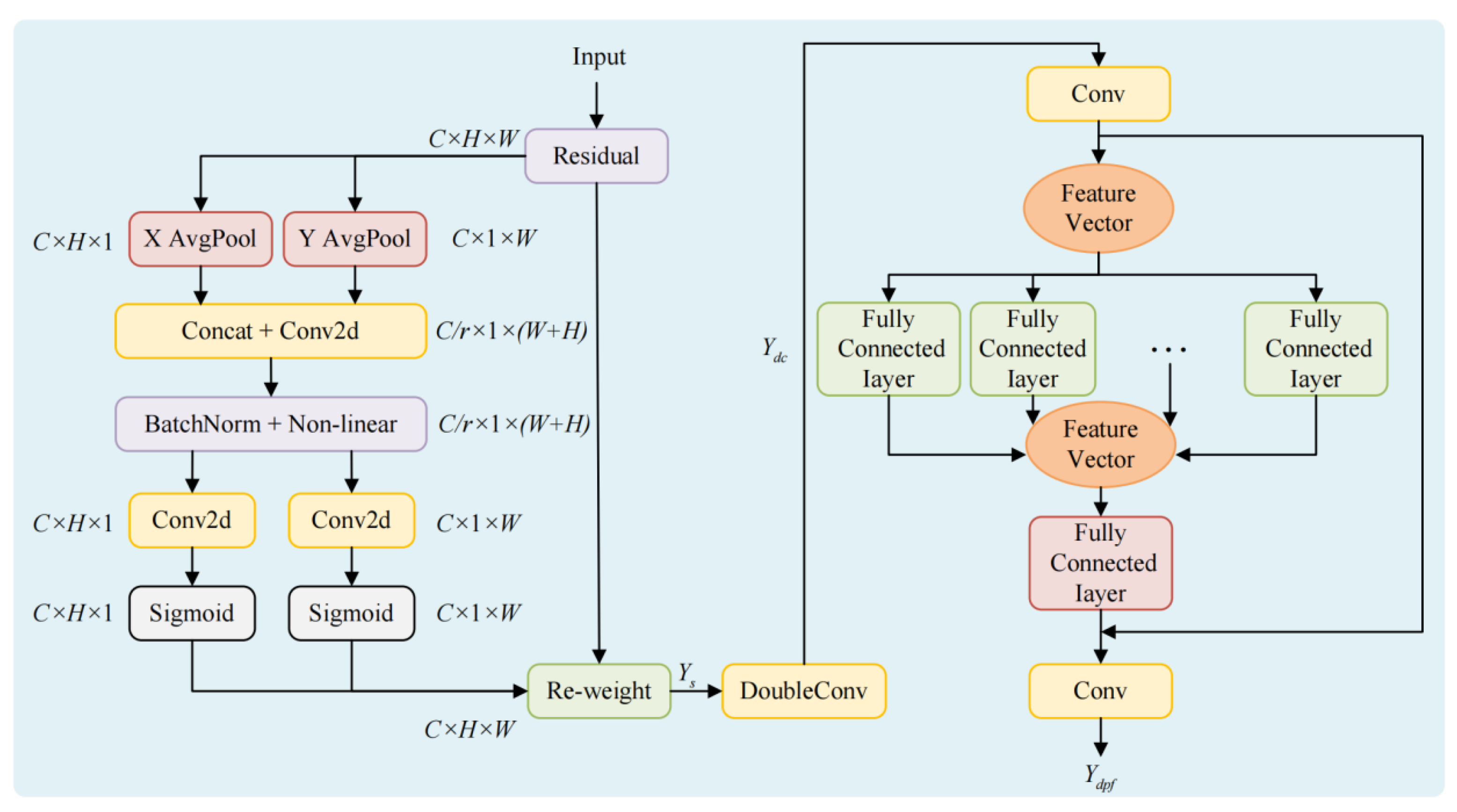
Figure 6.
Examples from the LoveDA dataset. (a)-(d): RGB tiles with a size of 1024×1024 pixels from urban and rural areas. The bottom row shows the corresponding pixel-level annotations, where each color represents a distinct land cover class. These annotations are used to assess the model’s ability to differentiate between various land types, including background, buildings, roads, water, barren areas, forests, and agriculture. The color legend is provided below for easy reference.
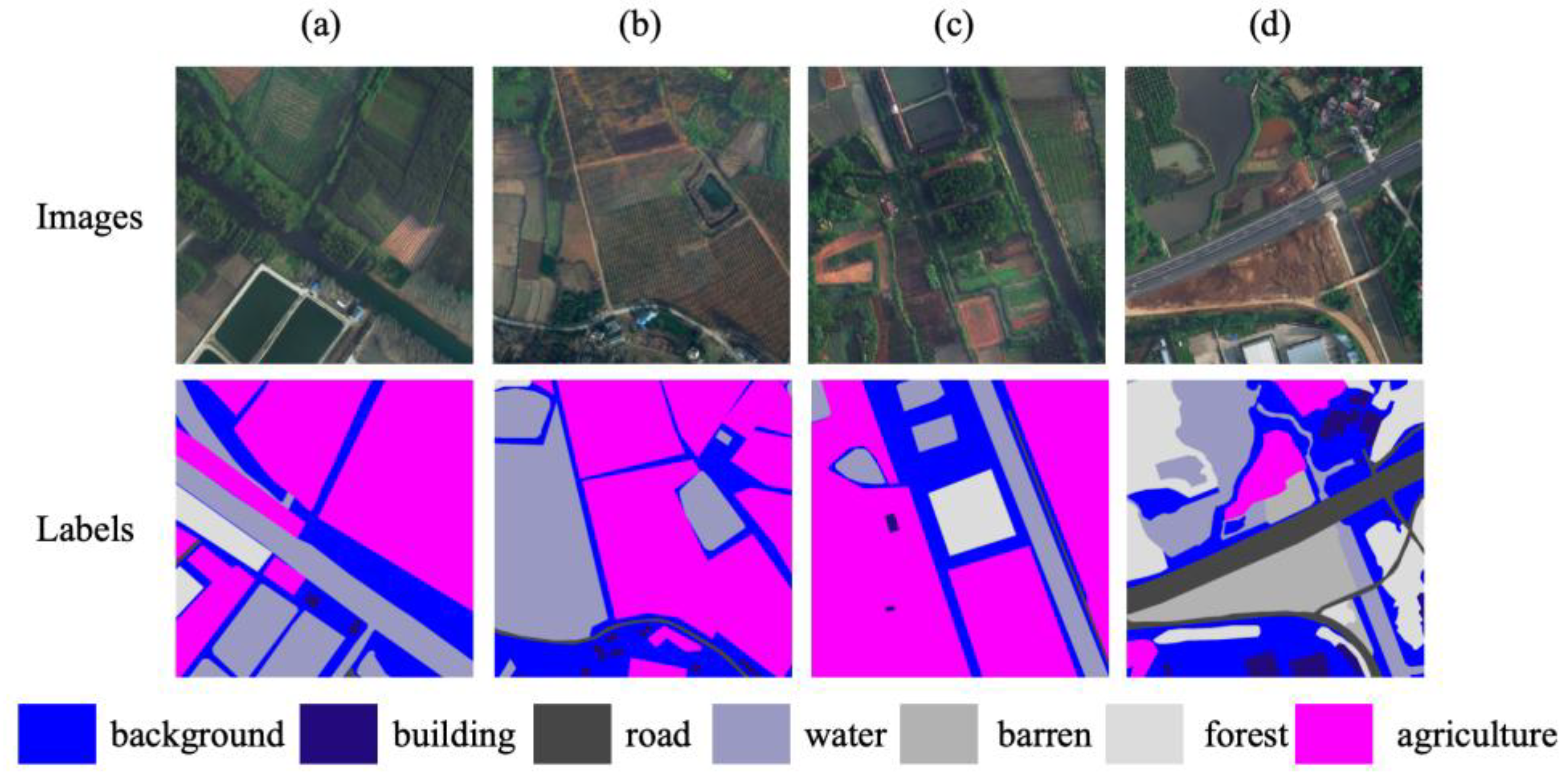
Figure 7.
Examples from the ISPRS Potsdam dataset. (a)-(d): IRRG tiles with a ground sampling distance of 5 cm and a typical size of 6000×6000 pixels from urban areas. The bottom row shows the corresponding pixel-level annotations for the six classes. Each color corresponds to a different class, as indicated by the legend below the images.
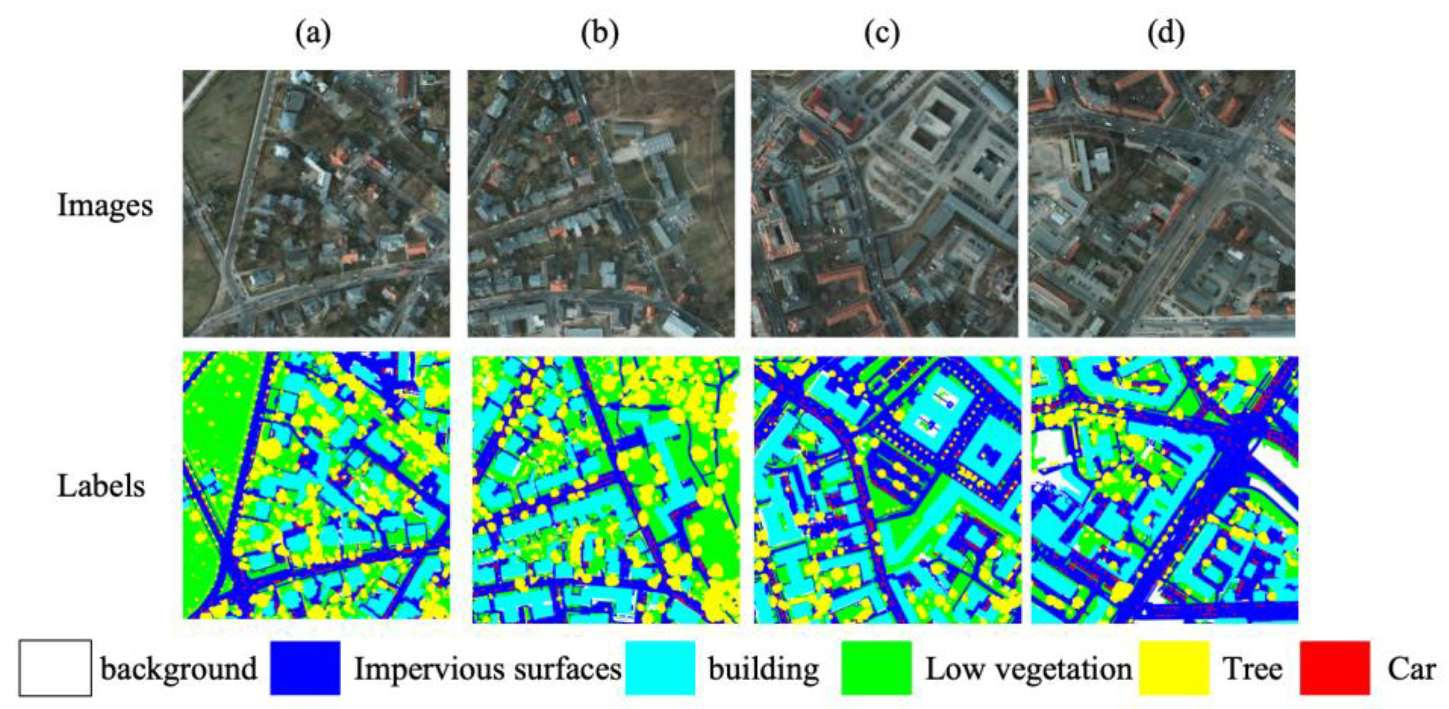
Figure 8.
Qualitative comparisons on the LoveDA dataset. (a)-(e): Representative urban and rural tiles. Columns: Image, Label, BiSeNetV2, ConvNeXt + UPerNet, PSPNet (ResNet-18), ResUNet, SegFormer-B0, Swin-T + UPerNet, DeepLabV3+ (ResNet-18), and LGD-DeepLabV3+ (ours). LGD-DeepLabV3+ demonstrates improved continuity of thin roads and rivers, clearer building boundaries under shadows, and fewer barren-water misclassifications compared to the baselines.
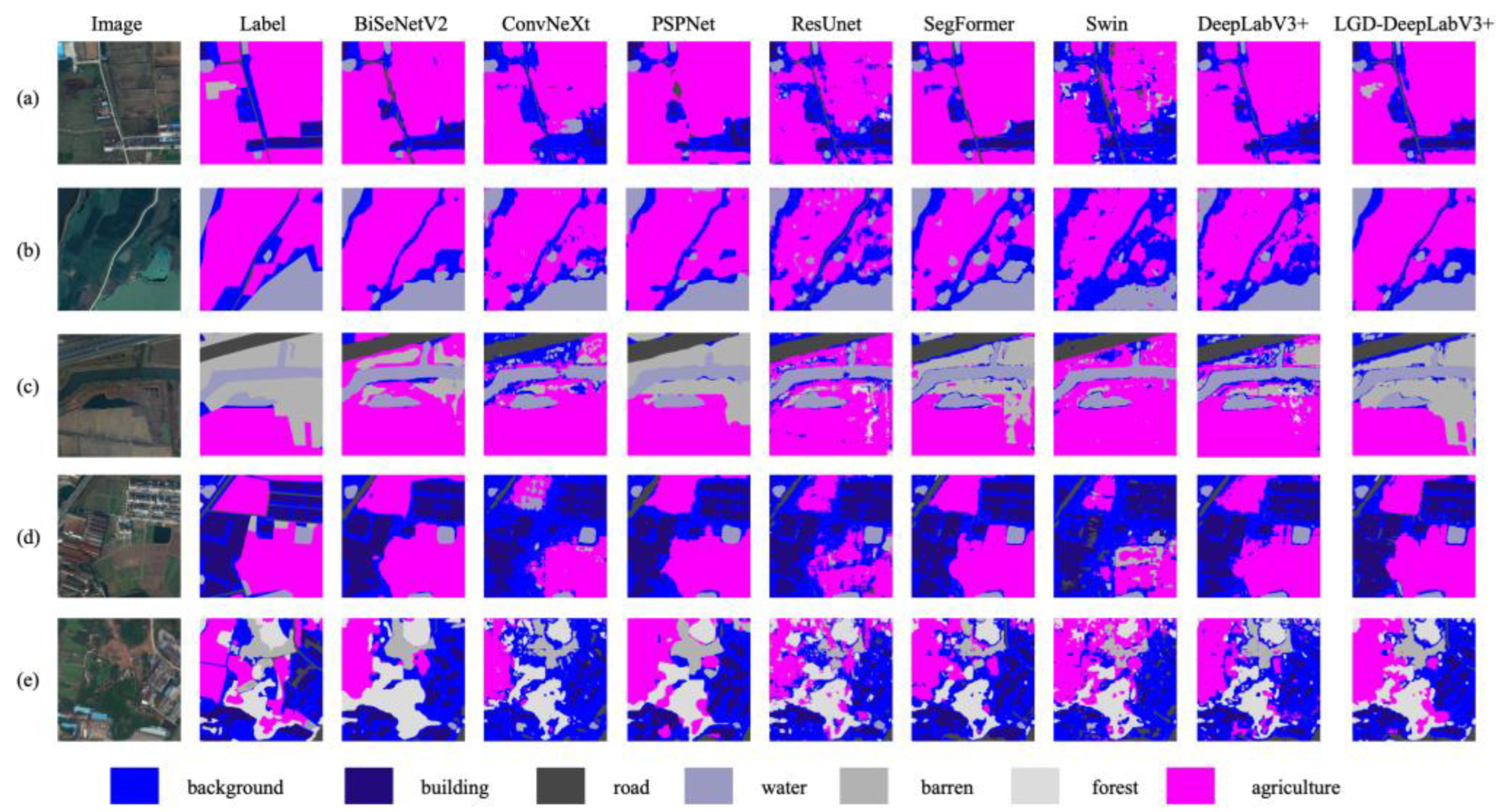
Figure 9.
Qualitative comparisons on the Potsdam dataset. LGD-DeepLabV3+ demonstrates improved segmentation performance, particularly in the continuity of road and river networks, clearer building boundaries under shadows, and reduced barren-water misclassifications. The color legend below indicates the corresponding land cover classes.
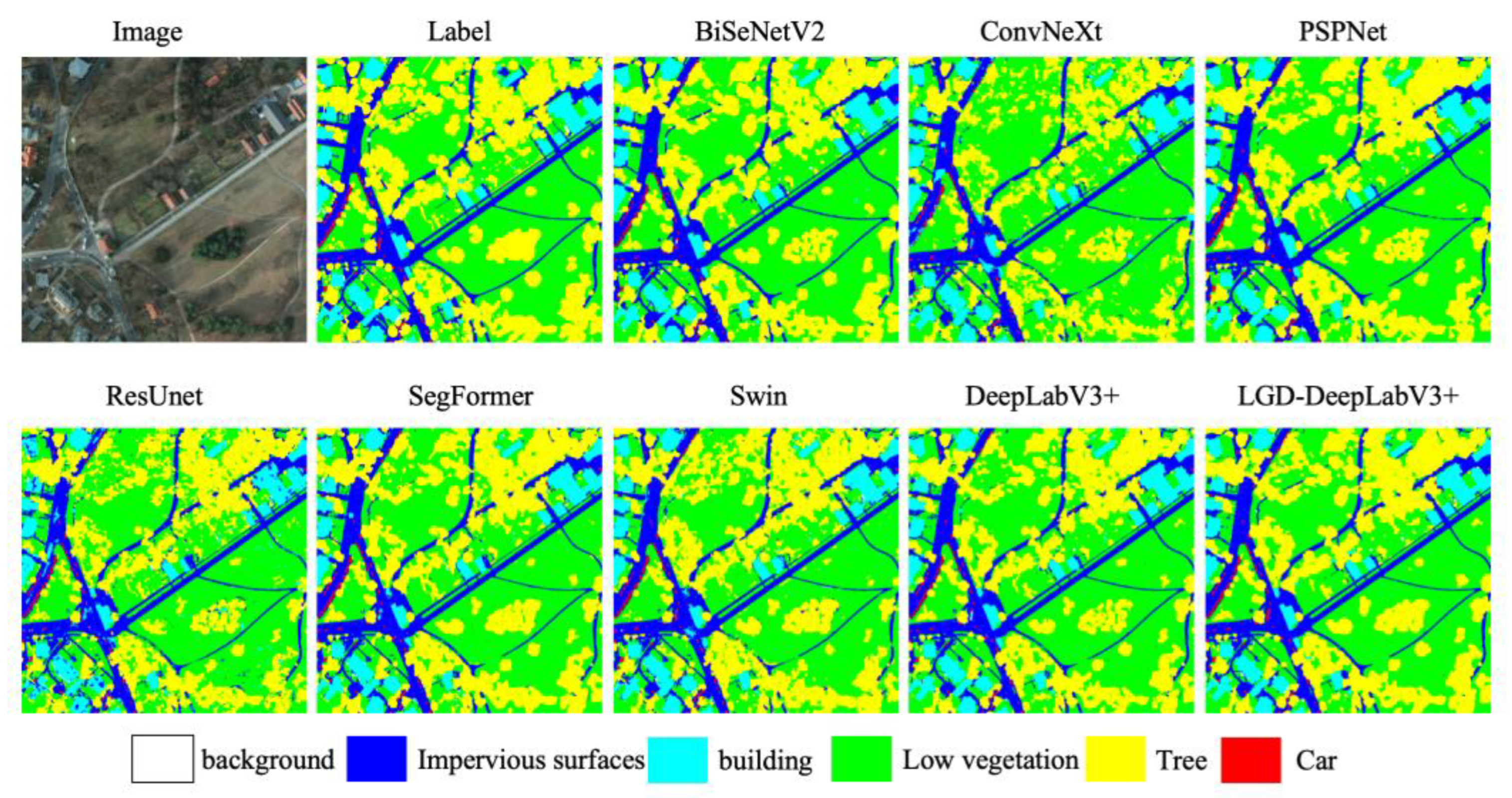

Table 1.
Model training parameters for LoveDA and ISPRS Potsdam.
| Parameter | LoveDA | ISPRS Potsdam |
|---|---|---|
| Epochs | Iter-based(50,000 iterations) | Iter-based(50,000 iterations) |
| Batch size | 4 | 4 |
| Image size | Train crop: 512×512 Val/Test source: 1024×1024 |
Train crop: 512×512 Val/Test source: 6000×6000 |
| Optimizer algorithm | Adam | Adam |
| Learning rate | 0.001 | 0.001 |
| Weight decay | 0.005 | 0.005 |
Table 2.
Comparison Experiments on the LoveDA Dataset.
| Ex | Model | Model Variant | OA(%) | mIOU(%) | mF1(%) |
|---|---|---|---|---|---|
| 1 | BiSeNetV2 | - | 73.58 | 54.36 | 69.91 |
| 2 | ConvNeXt | Tiny + UPerNet | 67.31 | 42.41 | 58.32 |
| 3 | PSPNet | Resnet-18 | 71.17 | 50.72 | 66.68 |
| 4 | ResUNet | - | 68.03 | 46.57 | 62.35 |
| 5 | SegFormer | B0 | 73.37 | 53.01 | 68.50 |
| 6 | Swin | Tiny + UPerNet | 63.95 | 39.14 | 55.23 |
| 7 | DeepLabV3+ | Resnet-18 | 71.39 | 49.65 | 65.48 |
| 8 | LGD-DeepLabV3+ | - | 76.32 | 58.48 | 73.37 |
Table 3.
LoveDA: Class-wise Comparison Between Baseline and LGD-DeepLabV3+.
| Class (K=7) | Baseline mIoU(%) |
LGD-DeepLabV3+ mIoU(%) |
Baseline mF1(%) |
LGD-DeepLabV3+ mF1(%) |
|---|---|---|---|---|
| background | 57.36 | 60.17 | 72.91 | 75.13 |
| building | 52.42 | 59.22 | 68.78 | 74.39 |
| road | 45.68 | 56.96 | 62.72 | 72.58 |
| water | 62.57 | 72.52 | 76.98 | 84.07 |
| barren | 25.81 | 43.68 | 41.03 | 60.80 |
| forest | 44.17 | 49.14 | 61.28 | 65.90 |
| agriculture | 59.55 | 67.56 | 74.64 | 80.70 |
Table 4.
Comparison Experiments on the ISPRS Potsdam Dataset.
| Ex | Model | Model Variant | OA(%) | mIOU(%) | mF1(%) |
|---|---|---|---|---|---|
| 1 | BiSeNetV2 | - | 88.16 | 76.16 | 86.16 |
| 2 | ConvNeXt | Tiny + UPerNet | 77.02 | 58.13 | 72.11 |
| 3 | PSPNet | Resnet-18 | 84.91 | 69.96 | 81.85 |
| 4 | ResUNet | - | 78.14 | 59.70 | 72.54 |
| 5 | SegFormer | B0 | 85.01 | 71.76 | 83.19 |
| 6 | Swin | Tiny + UPerNet | 79.67 | 63.53 | 76.88 |
| 7 | DeepLabV3+ | Resnet-18 | 86.72 | 74.07 | 84.60 |
| 8 | LGD-DeepLabV3+ | - | 90.34 | 80.79 | 89.16 |
Table 5.
ISPRS Potsdam: Class-wise Comparison Between Baseline and LGD-DeepLabV3+.
| Class (K=6) | Baseline mIoU(%) |
LGD-DeepLabV3+ mIoU(%) |
Baseline mF1(%) |
LGD-DeepLabV3+ mF1(%) |
|---|---|---|---|---|
| background | 54.16 | 70.73 | 70.26 | 82.85 |
| Impervious surfaces | 82.72 | 88.50 | 90.54 | 93.90 |
| Building | 89.99 | 93.51 | 94.73 | 96.65 |
| Low vegetation | 71.32 | 76.54 | 83.26 | 86.71 |
| Tree | 69.25 | 74.47 | 81.83 | 85.37 |
| Car | 76.99 | 81.02 | 87.00 | 89.51 |
Table 6.
Ablation Results on LoveDA, with values from the validation set; Δ represents the percentage improvement relative to the baseline.
Table 6.
Ablation Results on LoveDA, with values from the validation set; Δ represents the percentage improvement relative to the baseline.
| Ex | Method | OA(%) | mIOU(%) | mF1(%) | ΔmIOU(pp) | ΔmF1(pp) |
|---|---|---|---|---|---|---|
| 1 | DeepLabV3+ | 71.39 | 49.65 | 65.48 | - | - |
| 2 | +LISModule | 74.62 | 55.48 | 70.76 | +5.83 | +5.28 |
| 3 | +GCRModule | 74.73 | 56.07 | 71.32 | +6.42 | +5.84 |
| 4 | +DPFModule | 75.05 | 56.78 | 71.94 | +7.13 | +6.46 |
| 5 | LGD-DeepLabV3+ | 76.32 | 58.48 | 73.37 | +8.83 | +7.89 |
Table 7.
Ablation Results on ISPRS Potsdam, with values from the validation set.
| Ex | Method | OA(%) | mIOU(%) | mF1(%) | ΔmIOU(pp) | ΔmF1(pp) |
|---|---|---|---|---|---|---|
| 1 | DeepLabV3+ | 86.72 | 74.07 | 84.60 | - | - |
| 2 | +LISModule | 88.75 | 77.54 | 86.98 | +3.47 | +2.38 |
| 3 | +GCRModule | 89.44 | 79.15 | 88.10 | +5.08 | +3.50 |
| 4 | +DPFModule | 89.39 | 78.97 | 87.97 | +4.90 | +3.37 |
| 5 | LGD-DeepLabV3+ | 90.34 | 80.79 | 89.16 | +6.72 | +5.01 |
Table 8.
Comparison of Complexity and Efficiency.
| DataSet | Method | Params(M) | GFLOPs(G) | Latency(ms) | FPS | PeakMem(GB) |
|---|---|---|---|---|---|---|
| LoveDA | Baseline | 24.90 | 23.34 | 4.53 | 220.79 | 0.280 |
| LoveDA | +GCRModule | 103.66 | 43.50 | 6.15 | 162.51 | 0.575 |
| LoveDA | LGD-DeepLabV3+ | 110.18 | 136.12 | 26.65 | 37.53 | 1.541 |
| Potsdam | Baseline | 24.89 | 23.33 | 4.50 | 222.12 | 0.277 |
| Potsdam | +GCRModule | 103.66 | 43.49 | 5.62 | 178.05 | 0.575 |
| Potsdam | LGD-DeepLabV3+ | 110.18 | 136.11 | 26.70 | 37.46 | 1.541 |
Disclaimer/Publisher’s Note: The statements, opinions and data contained in all publications are solely those of the individual author(s) and contributor(s) and not of MDPI and/or the editor(s). MDPI and/or the editor(s) disclaim responsibility for any injury to people or property resulting from any ideas, methods, instructions or products referred to in the content. |
© 2026 by the authors. Licensee MDPI, Basel, Switzerland. This article is an open access article distributed under the terms and conditions of the Creative Commons Attribution (CC BY) license (http://creativecommons.org/licenses/by/4.0/).
Copyright: This open access article is published under a Creative Commons CC BY 4.0 license, which permit the free download, distribution, and reuse, provided that the author and preprint are cited in any reuse.


