
Submitted:
20 January 2026
Posted:
21 January 2026
You are already at the latest version
Abstract
Hierarchical triple systems (HTSs), composed of an inner compact binary and a distant tertiary companion, can undergo secular interactions that induce Kozai–Lidov (KL) oscillations. These oscillations can drive the inner binary to high eccentricities, substantially enhancing its gravitational wave (GW) emission. In this work, we simulate the evolution of such systems using the N-body integrator REBOUND, selecting astrophysical models from constrained parameter spaces that are likely to exhibit KL dynamics. To assess detectability, we employ tools such as EccentricFD to model GW signals from these eccentric binaries, varying mass ratios and eccentricities across detectors, including LIGO, LISA, and LGWA. Our results highlight the influence of general relativistic corrections at 1PN order on the suppression or modulation of KL cycles and suggest the existence of an additional dynamical constraint governing HTS stability. We find that GW signals from such systems are within the sensitivity range of both current and future detectors. This study underscores the role of three-body dynamics in shaping GW observables and provides a foundation for the development of waveform templates for eccentric sources.
Keywords:
gravitational waves
; hierarchical triple system
; LIGO
; LISA
; LGWA
1. Introduction
The existence of gravitational waves (GWs) was first predicted theoretically by Einstein using his theory of General Relativity (GR) [1]. Unlike electromagnetic radiation, GWs are produced by quadrupole sources rather than dipoles, allowing Einstein to describe the rate of energy loss due to GW emission. GWs arise from perturbations in the spacetime metric caused by asymmetries such as binary systems, deformations in compact objects like neutron stars (NSs), or density fluctuations during inflation. The GW signal is typically classified into three phases: inspiral, merger, and ringdown. During inspiral, a compact binary slowly loses energy via GW emission, increasing in frequency and amplitude. The merger produces the peak GW signal as the objects coalesce, followed by the ringdown, dominated by the relaxation of the remnant and emission of decaying quasinormal modes [2].
The first direct GW detection occurred in 2015 when LIGO observed GW150914 from a binary black hole merger [3], opening a new era of GW astronomy. Ground-based interferometers like LIGO, Virgo, and KAGRA (forming the LVK collaboration) currently operate in the 10 Hz–10 kHz range and have detected over 100 compact object mergers. However, signals below 10 Hz remain inaccessible, motivating larger ground-based detectors such as the 40 km Cosmic Explorer and Einstein Telescope, as well as space-based observatories like the Laser Interferometer Space Antenna (LISA) [4] and the Lunar Gravitational Wave Antenna (LGWA) [5]. These extended sensitivities are crucial for detecting eccentric binaries, whose GW emission is distributed over multiple harmonics and is more efficient than that from circular orbits [6,7]. The total radiation power P averaged over one orbital period is given by
where and are the semi-major axis and the eccentricity of the inner binary, respectively. It shows that the radiation power increases rapidly as the eccentricity increases. The total radiation power P is the sum of the power radiated in the nth harmonic , given as
where the is the power due to the nth harmonic. The peak of the spectrum is given by
where is the orbital frequency of the inner binary and is the magnification factor, which represents the number of harmonics. This factor can be approximated, in the range [6,8], to
We can see that if eccentricity , , describing the peak frequency of GWs from a circular orbit, whereas for high eccentricities, is very high and would be in the detectable range of the detector (Hz to 10kHz). Also, since the signal from a highly eccentric orbit consists many harmonics, the signal has a broad spectrum of frequencies. We also check the strain of the wave at the nth harmonic, given by
where is the frequency of nth harmonic, D is the distance of the source. At , we can approximate the equation and express in scaled form as
For ,
which is highly detectable in our present and future detectors. Eccentric binaries are highly efficient GW emitters and hence appear at lower frequencies compared to circular orbits. These kinds of eccentric systems must dominate the detections compared to circular orbit system but due to the circularization of the eccentric orbit by GW emission, by the time of merger, the orbit has almost completely circularized, causing it to appear in the LVK band as a binary in a circular orbit. Some residual eccentricity may remain, but has a very negligible effect on the signal.
The formation of eccentric orbits can result from dynamical interactions with multiple bodies, particularly through the Kozai-Lidov (KL) mechanism in hierarchical triple systems (HTSs). The KL mechanism [9,10], independently identified by Yoshihide Kozai and Mikhail Lidov in the 1960s, occurs when a tertiary companion perturbs an inner binary, causing periodic exchanges between its eccentricity and inclination over timescales much longer than the orbital period. This interplay produces long-term modulations in both the inner binary’s eccentricity and the angular displacement between the inner and outer binaries.
Analytically, the Hamiltonian of a hierarchical triple system can be decomposed into contributions from the inner and outer binaries, along with a term representing their mutual interaction [11]:
This decomposition allows separate treatment of the inner and outer binary evolutions while capturing the essential perturbative effects that drive KL oscillations.
In the context of gravitational-wave (GW) astrophysics, the KL mechanism is significant because it can maintain high eccentricities () for binaries entering the LIGO detection range, which may accelerate merger times. Simulations suggest that a substantial fraction of binaries in dense stellar environments are influenced by third-body perturbations, making accurate modeling of their dynamics essential. This requires integrating third-body interactions along with post-Newtonian relativistic corrections [11], especially when predicting merger rates of eccentric binaries.
A fundamental assumption in this configuration is that the tertiary’s gravitational influence on the inner binary is weaker than the interaction between the two inner bodies. In a simple two-body Newtonian system, a bound orbit is elliptical and characterized by six orbital elements (). In hierarchical triples, perturbations from the tertiary lead to deviations from these idealized ellipses, affecting both the inner binary’s orbital shape and orientation over time [6].
To account for these perturbations, the concept of an osculating orbit [12] is introduced, providing an approximate trajectory that can be described by an elliptical path defined by the aforementioned six orbital elements, derived from the system’s instantaneous position and velocity at any given moment. As for the outer orbit, this is considered as the motion of the inner binary’s center of mass as it rotates around the tertiary companion, which can also be represented as another osculating orbit. In this framework, the masses of the inner binary components are denoted and , while the tertiary companion has a mass . To distinguish between the inner and outer orbits, subscripts "in" and "out" are used respectively. In such systems, the orbital periods of the inner and outer binary is given by
At a particular relative inclination I, a secular change of orbital elements may occur where under certain conditions, an oscillation between the values of the eccentricity and relative inclination occurs with the relative equation defined as the argument between the inner and outer orbital planes [9,10] and is given by
which results in the secular exchange of and I with the conserved value [13] of
with the condition for the KL oscillation, provided that and the outer orbit is circular.
Note that the KL oscillation will occur even if is not much smaller than , . The KL oscillation timescale [14] is given by
When modeling an HTS system, we must also consider the general relativistic precession in the system and the Lense-Thirring, (LT) effect, which is a general relativistic correction to the precession of a gyroscope in the presence of a large rotating mass. This causes the relative orbital nodes of the gyroscope to precess[15]. Recent studies have shown changes in KL oscillations caused due to GR effects involving a SMBH. If the third body is a rapidly rotating SMBH, then LT effect might become important in changing the evolution of eccentricity excitation from the usual KL oscillation. The effect appears in the 1.5PN order [16,17,18]. For a rotating black hole, the spin angular momentum [6,16,18] is given as , where is the spin parameter, and the outer orbital angular momentum [16,18] is given as
where M is the total mass of the gyroscope and the reduced mass of the outer orbit is defined by
The timescale of the orbit-averaged precession of around [16,18] is given by
This study focuses on developing a more accurate model for GW emission from HTSs by conducting a preliminary study on the detectability of such systems in our present and future detectors and providing a theoretical framework for the evolution of the system and modeling the GWs.
2. HTS Simulation
2.1. Constraints
2.1.1. Stability of Hierarchical System
For KL oscillations to occur, the stability of the three body system must be maintained. For this reason, a necessary criteria is mentioned in [19], which predicts a minimum separation between the inner and outer orbits for stability, beyond which the system might become chaotic. This condition is given by
This gives us a lower bound for the separation between the two orbits.
2.1.2. Relativistic Precession of Periastron
KL oscillations are suppressed or maximum eccentricity is restricted by the periastron precession of inner binary. To constrain this effect, we consider the GR precession timescale of periastron [6,20] of the inner binary and compare it with the KL timescale (see Equation (1.13)) to get the constraint whose scaled expression is of the form
2.1.3. Lense-Thirring Precession Effect
For the Lense - Thirring effect to appear, we need to have a constraint such that (see Equation (1.16)), for which the scaled expression [6] is given as
assuming
2.2. Parameter Space and Final Models
We set up 17 mass combinations (see Table 1) and then for each combination, using the constraints, we find the region of stability (shown in Figure 1) and select the and of each model. Based on these initial models, we find all the initial parameters for these models (see Table 2). Note that we haven’t considered triple stellar mass HTS due to the possibility of their formation being much lower.
We shall use these parameters in the simulation to verify its working process and confirm the effects of KL dynamics occurring in these systems.
2.3. Modeling a Simple 3-Body System Using REBOUND
To simulate the dynamical evolution of HTSs, we used the open-source N-body integrator REBOUND [21]. REBOUND is widely adopted in astrophysical research for its flexibility, modular architecture, and high-precision integrators suitable for simulating gravitational interactions over a wide range of dynamical regimes. In particular, it supports various integration schemes, collision detection algorithms, and allows for custom initial conditions and external forces. All the integrators work on the basis of the Drift-Kick-Drift (DKD) scheme. The Hamiltonian of the system is given by , where and represent the kinetic and potential parts, respectively. The DKD scheme integrates over a timestep, say dt, where half the timestep is used to integrate the kinetic part and the other, the potential part. For this study, we used the built-in integrator, IAS15 [22]. It is a 15th-order non-symplectic integrator (Newtonian) that can handle both conservative and non-conservative forces.
Our HTS are setup by initializing our masses alongside their respective parameter using the code. We then choose our time period over which to integrate the system and also the timestep to be used by the REBOUND integrator. In this case, we have kept the default timestep, . The code uses a loop to capture the positions and velocities of the masses in the system over the given time period over intervals of time determined by the required resolution for analysis. In all cases, resolution has been set to 500000. Hence, the number of time intervals is 500000. The extracted positions and velocities are used to calculate the eccentricity and inclination of the inner binary. This code makes up the Newt3 code.
We shall use REBOUNDx [23] to add additional physical effects, such as 1PN corrections, tidal forces, which can be incorporated using the REBOUNDx extension library. The 1PN correction to the Newtonian N-body Hamiltonian used by REBOUND can be easily augmented onto Newt3 by attaching the gr_full module to the same code. This module, during a simulation run, calculates the corrections using the instantaneous values of positions, velocities and modifies the accelerations of the masses at each timestep. This allows us to see the effect of GR precession on our system and how it affects our KL effect. This addition of the gr_full module to the Newt3 code creates the GR3 code. We shall discuss the results of our simulations in Section 4.
3. Detectability of HTS Through GWs
The noise curves of detectors play a crucial role in determining the detectability of various sources. These curves illustrate the sensitivity of the detector across different frequency ranges, providing valuable insights into its performance. To obtain these noise curves, we analyze noise measurements collected by sensors in the time domain. By performing a Fast Fourier Transform (FFT) on this data, we can calculate the Power Spectral Density (PSD) of the noise. Alternatively, an analytical equation for the noise specific to the detector can also be employed. For our purposes, the analytical noise proves to be sufficient, allowing us to effectively assess the detector’s capabilities.
3.1. LISA
The Laser Interferometer Space Antenna (LISA) [24] is an ambitious gravitational wave observatory set to be launched by the European Space Agency (ESA), with participation from NASA, targeting an operational period in the 2030s. Unlike ground-based detectors like LIGO and Virgo, LISA will operate in space, allowing it to detect GWs at much lower frequencies. It comprises three spacecraft arranged in an equilateral triangle with 2.5 million kilometers between each pair [25]. LISA is designed to capture GWs produced by massive celestial events, such as mergers of supermassive black holes, inspirals of stellar-mass compact objects into supermassive black holes, and potentially signals from the early universe.
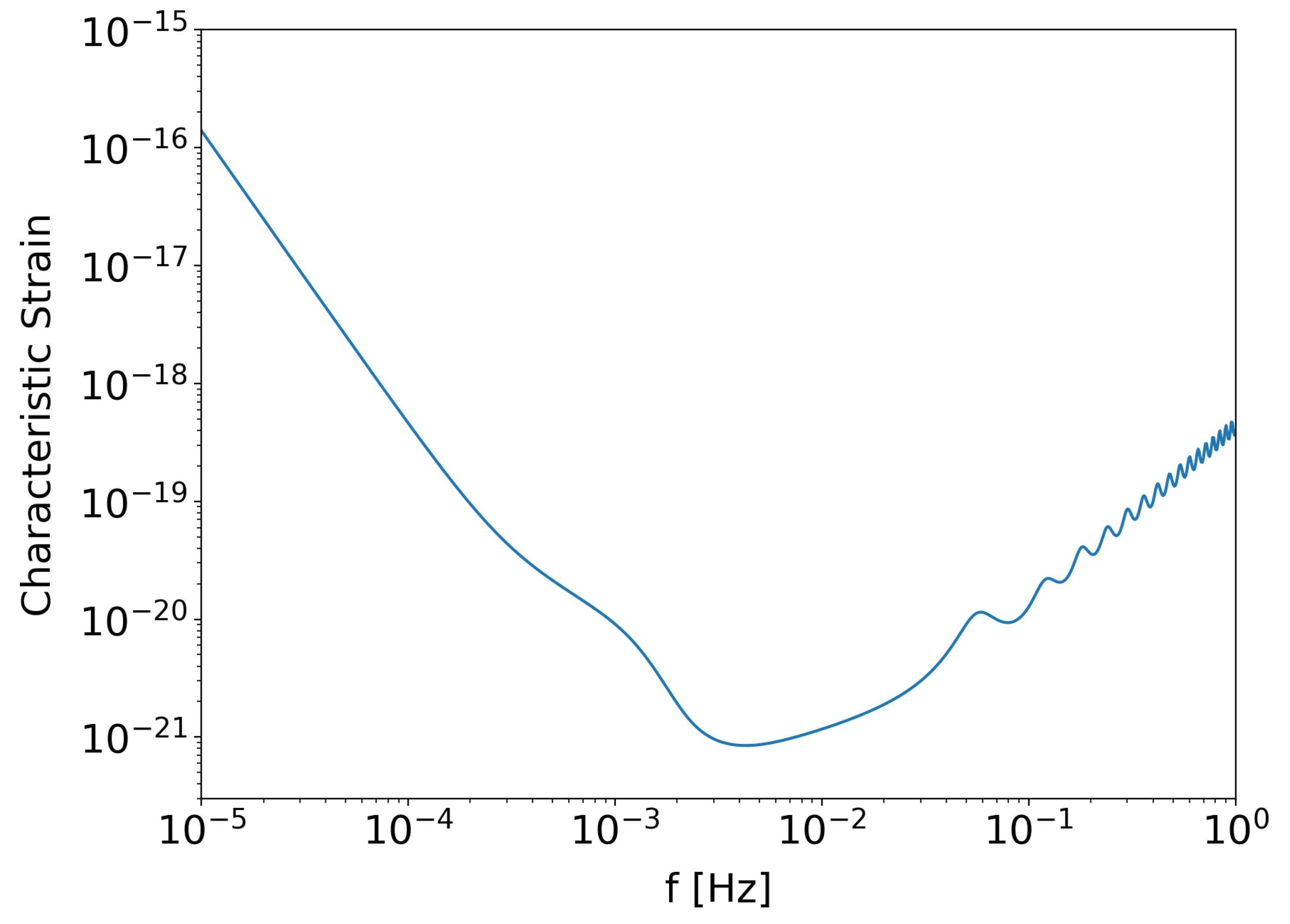
LISA’s low-frequency sensitivity opens a window to events beyond the reach of current ground-based interferometers. These events can reveal crucial insights into galaxy formation, cosmology, and fundamental physics. Orbiting the Sun in tandem with Earth, LISA’s constellation will effectively remove terrestrial noise sources, providing a pristine environment for GW detection. The data from LISA will complement observations from high-frequency detectors on Earth, expanding our understanding of the universe through multi-frequency GW astronomy. The sensitivity curve for LISA [25] is given by
where is the power spectral density of the noise, and is the response function of the detector.
Here, is given by,
where is the single optical metrological noise, and is the single test mass acceleration noise.
And, the response function is given by,
Thus, the sensitivity curve is
where and .
Figure 2.
Sensitivity curve of the LISA detector.
3.2. LGWA
The Lunar Gravitational-wave Antenna (LGWA) is a pioneering gravitational-wave observatory proposed for deployment on the Moon. Unlike space-based interferometers such as LISA, LGWA utilizes the Moon itself as a giant solid-state antenna for detecting GWs (GWs). The mission concept involves an array of high-precision inertial sensors—Lunar Inertial Gravitational-wave Sensors (LIGS)—deployed in permanently shadowed regions (PSRs) at the lunar poles, where seismic noise is minimal and thermal conditions are extremely stable [5].
LGWA is designed to be sensitive in the decihertz frequency band, spanning from about 1 mHz to 1 Hz. This band bridges the gap between the millihertz sensitivity range of space-based detectors like LISA and the hertz–kilohertz range of ground-based detectors such as the Einstein Telescope and Cosmic Explorer. The lunar environment—with its cryogenic temperatures, lack of atmosphere, and seismic quietness—provides a uniquely favorable platform for low-frequency GW detection that cannot be achieved on Earth.
Through its novel detection mechanism, LGWA is expected to observe GWs from a wide range of astrophysical and cosmological sources. These include inspirals and mergers of intermediate-mass black hole binaries, binary white dwarf systems, and potentially the early inspiral phases of binary neutron stars and stellar-origin black holes, enabling early warnings for electromagnetic follow-up. LGWA also holds promise for detecting unmodeled transients such as tidal disruptions of white dwarfs, and constraining the cosmological stochastic GW background.
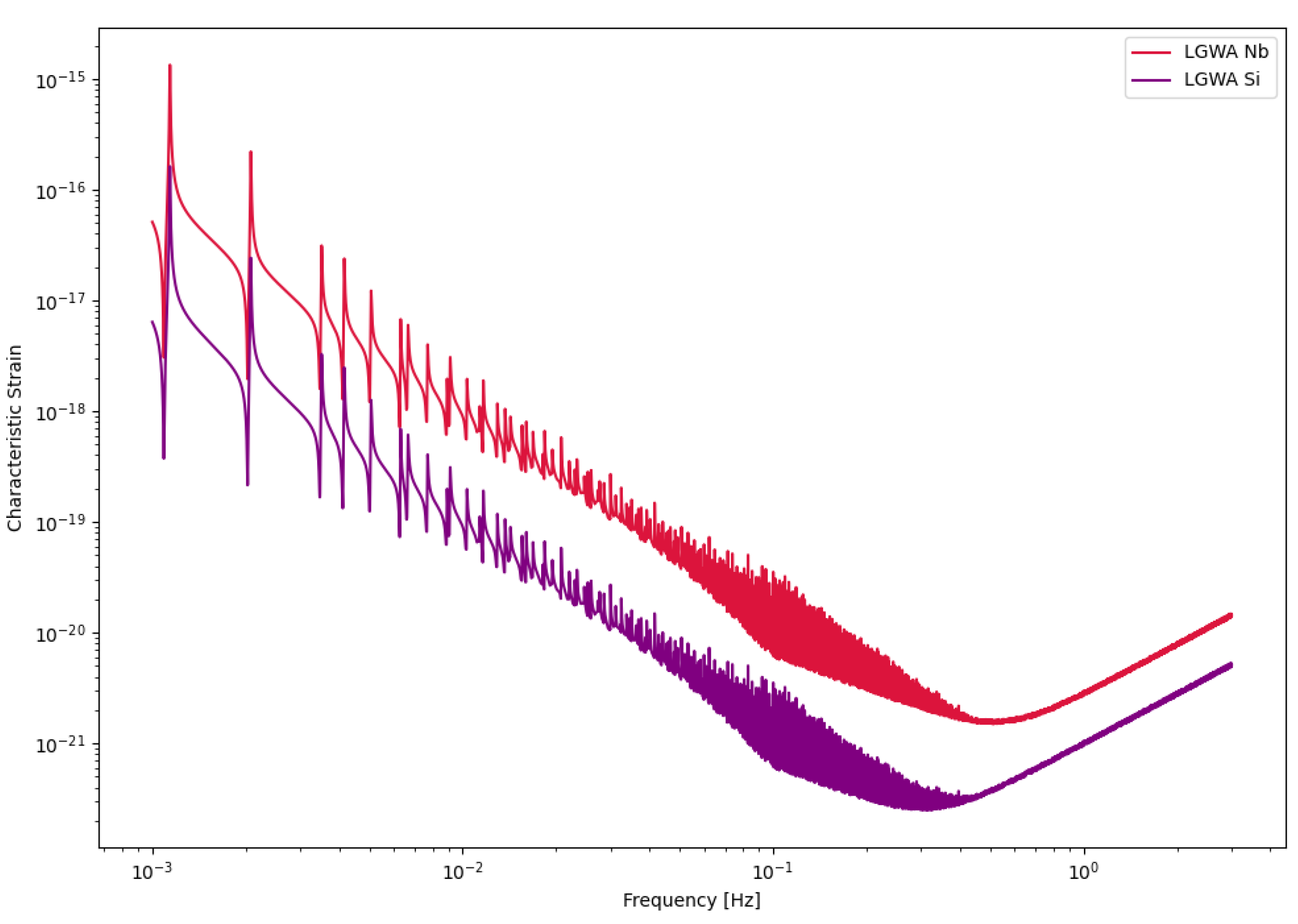
Unlike traditional interferometers, LGWA measures the Moon’s elastic response to passing GWs. Its sensitivity is characterized by the displacement noise of its inertial sensors and the Moon’s GW response function.
Figure 3.
Sensitivity curves of the LGWA detector.
3.3. EccentricFD
EccentricFD is a frequency-domain waveform model implemented in the PyCBC library for simulating gravitational wave (GW) signals from eccentric binary systems. Unlike traditional quasi-circular approximants, EccentricFD includes the effects of non-zero eccentricity at leading-order post-Newtonian (PN) accuracy, enabling the modeling of binaries formed through dynamical capture, globular cluster interactions, or hierarchical triple-induced Kozai–Lidov oscillations. These systems may retain measurable eccentricities within the LIGO–Virgo–KAGRA frequency band, and waveform models such as EccentricFD are crucial for their detection and characterization [26,27,28]. The model is computationally efficient due to its frequency-domain implementation and is widely used for injection studies and parameter estimation in the analysis of non-circular compact binary coalescences.
The construction of the EccentricFD model is based on the stationary phase approximation, where the waveform is expressed as a sum over harmonics of the orbital frequency. The amplitude and phase of each harmonic are modified by the orbital eccentricity, which is specified at a reference frequency, typically 10 Hz. The model incorporates post-Newtonian corrections up to 3PN order in the binary’s orbital energy and gravitational wave flux. It takes as input the component masses, reference eccentricity, and luminosity distance, and returns the frequency-domain plus and cross polarizations [27,28].
This waveform model is used to get the frequency-domain waveform of the inner binaries from our various models and are then plotted onto the sensitivity curves of LISA and LGWA to identify whether the signal will be detectable in the detector. However, since we do not have access to the waveform response of LISA and LGWA, these plots just provide us the rough estimates of their detectability.
4. Results and Discussion
4.1. Simulations
We have run the initial parameters of our models (see Section 2.2, Table 2) through our Newtonian three-body code, Newt3, and our first-order Post Newtonian (1PN) GR three-body code, GR3. In most cases, we see that inclusion of GR at 1PN order increases the number of cycles observed over a certain period. In some cases, the system is stable but no KL oscillations occur and in others, the system is chaotic. We divide our simulation results based on their stability and the occurrence of KL oscillation in the HTS in order to understand the effects occurring in these systems much more clearly.
4.1.1. Stable HTS with KL Oscillation
From our simulations, we see that systems IM1, IM2, IM3 (see Figure 4) show negligible difference in the number of KL cycles occurring when simulated at both Newtonian and 1PN level through the Newt3 and GR3 codes, respectively.
But as soon as the tertiary mass range goes into the SMBH range, we see large changes in the simulation results given at Newtonian and 1PN order, as seen in systems SM1, SM2, SM3, SM6, SM7 (see Figure 5). In SM6 and SM7, we also see that in the GR3 simulation result, there appears to be a lot more fluctuation in the eccentricity of inner binary, as it approaches the maximum eccentricity allowed by the KL mechanism.
In the case of system SM4, we see a drastic difference in the number of KL cycles (see Figure 6). This could be due to the initial mutual inclination, , being quite close to the lower limit of the effective limit range of mutual inclination for KL oscillations to occur.
4.1.2. Stable System But No KL Oscillation
We observe a curious case in system IM4 (see Figure 7). When simulated (over 20 years), we see that in both simulations, the inner binary does not exhibit any KL oscillations but the system is stable. The results from GR3 show that the inner binary is precessing at a wider angle about the tertiary compared to the Newt3 results, clearly seen in the simulation run for 200 years
4.1.3. Instability in Triple System
Systems IM4, IM5 and SM9 exhibit unstable, chaotic behaviour despite us considering parameters that are supposed to describe stable HTSs. In system I5, we see that all three bodies are unbounded in under 5 years whereas in systems SM9, the inner binary is ejected from the system instead of the creation of an unbounded system (see Figure 8).
4.2. Eccentric System Detectability
From our GW frequency domain plots (see Figure 9), we see that all our models come under the LISA band when considering their eccentricity to be very high. We also see that as eccentricity reduces, the signal comes towards the LIGO band. And since we know that binaries at high eccentricities circularize faster, we would be able to see their complete evolution over the LISA, LGWA and LIGO bands.
From Figure 10, we see that as eccentricity reduces, so does the number of harmonics observed in the band as a consequence of equation (1.1) and as a result, decreasing power loss from the system with decreasing eccentricity.
We can also consider future ground based detectors such as the Einstein Telescope (ET) [29] into the picture to create a continuous detector array for analyzing the complete evolution of the inner binary (see Figure 11). These detectors will allow us to capture the residual harmonics from the binary as its orbit circularizes.
5. Conclusion
This study investigates the dynamical evolution of hierarchical triple systems (HTSs) and evaluates their gravitational wave (GW) detectability through numerical simulations. By selecting models from astrophysically relevant parameter spaces and implementing them using REBOUND and REBOUNDx, we confirm the occurrence of KL oscillations and examine the competing influence of general relativistic (GR) precession. Our results highlight the importance of including post-Newtonian corrections, as GR precession can significantly modulate both the timescales and amplitude of KL-driven eccentricity growth. Interestingly, despite choosing initial parameters expected to yield stable HTSs displaying KL oscillations, our simulations reveal both stable and unstable systems.
Within the stable systems, two distinct behaviors emerge: systems exhibiting KL oscillations and systems that do not. For systems showing KL oscillations, the impact of including 1PN dynamics increases with the tertiary mass, particularly in the supermassive black hole (SMBH) regime, where KL oscillations become more frequent. This effect arises because GR precession can partially restart the KL mechanism even under imposed constraints, though its influence is weak [11].
We also identify notable outliers in our simulations. A stable system (IM4) does not display KL oscillations, while two unstable systems (IM5 and SM9) show unexpected chaotic behavior. In these cases, one inner binary mass is an order of magnitude larger than the other, but the tertiary mass differs: in the stable system, it is two orders of magnitude larger, whereas in the unstable systems, it is only one order larger. This suggests the existence of an additional stability constraint dependent on the mass ratios within the HTS. The stable system may lie within this constraint, explaining its stability and absence of KL oscillations, whereas the chaotic systems exceed it. Future work should aim to quantify this constraint to deepen our understanding of HTS stability.
From frequency-domain gravitational waveforms obtained using EccentricFD, we find that highly eccentric binaries driven by KL oscillations can emit GWs detectable by both current and future detectors. Specifically, LISA is well-suited to capture signals during the high-eccentricity inspiral phase, while aLIGO is more sensitive to the circularized final mergers. Proposed detectors such as LGWA, with a frequency band bridging LISA and LIGO, alongside the Einstein Telescope (ET), could identify residual eccentricity in these systems. This multi-band detectability underscores the potential for HTS-originating binaries to serve as complementary probes across a wide range of GW frequencies.
We acknowledge that our simulations of hierarchical triple systems (HTSs) are idealized and do not capture all physical effects present in realistic astrophysical environments. Additionally, the gravitational waveform curves presented here do not incorporate the detector response functions, and thus do not reflect how these signals would appear in actual observational data. Nevertheless, this study provides a foundational framework for constructing more sophisticated gravitational wave (GW) templates that include complex three-body dynamics and relativistic corrections. Ongoing development of our HTS code is aimed at incorporating higher-order PN terms, up to at least 2.5PN, to better understand the interplay between KL oscillations, GW emission, and other secular effects. These improvements will ultimately support the generation of more accurate, time-evolving GW waveforms for inner binaries embedded in hierarchical triple systems.
Data sharing is not applicable to this article as no datasets were stored or separately generated during the study. All data were produced and utilized in real-time within the simulation code for analysis and were not saved externally.
The underlying code for this study is not publicly available but may be made available to qualified researchers on reasonable request from the corresponding author.
All authors declare no financial or non-financial competing interests.
Author Contributions
MC conceived the project, developed the methodology, implemented the core software, performed the analysis, and wrote the manuscript. AK supervised the research and contributed to the validation of the results. RS contributed a small portion of the parameter estimation code and wrote part of the introduction. All authors read and approved the final manuscript.
Data Availability
Data sharing is not applicable to this article as no datasets were stored or separately generated
during the study. All data were produced and utilized in real-time within the simulation code for analysis and
were not saved externally.
Code Availability
The underlying code for this study is not publicly available but may be made available to
qualified researchers on reasonable request from the corresponding author.
Acknowledgments
This study received no funding. The authors acknowledge the use of computational resources provided by the DST-FIST Computational Lab at CHRIST (Deemed to be University), Bengaluru, where all computations were carried out. Mukhil C. also acknowledges helpful discussions with peers during the course of this work.
Competing Interests
All authors declare no financial or non-financial competing interests.
References
- Einstein, A. Über Gravitationswellen. Sitzungsberichte der Königlich Preussischen Akademie der Wissenschaften 1918, pp. 154–167.
- Abbott, B.; et al. Observation of Gravitational Waves from a Binary Black Hole Merger. Physical Review Letters 2016, 116. [CrossRef]
- Ray, S.; Bhattacharya, R.; Sahay, S.; Aziz, A.; Das, A. Gravitational wave: Generation and detection techniques. International Journal of Modern Physics D 2023. [CrossRef]
- Thorpe, J.I.; et al. The Laser Interferometer Space Antenna: Unveiling the Millihertz Gravitational Wave Sky. In Proceedings of the Bulletin of the American Astronomical Society, 2019, Vol. 51, p. 77, [arXiv:astro-ph.IM/1907.06482]. [CrossRef]
- Ajith, P.; et al. The Lunar Gravitational-wave Antenna: mission studies and science case. Journal of Cosmology and Astroparticle Physics 2025, 2025, 108. [CrossRef]
- Gupta, P.; Suzuki, H.; Okawa, H.; Maeda, K.i. Gravitational waves from hierarchical triple systems with Kozai-Lidov oscillation. Phys. Rev. D 2020, 101, 104053. [CrossRef]
- Peters, P.C.; Mathews, J. Gravitational Radiation from Point Masses in a Keplerian Orbit. Phys. Rev. 1963, 131, 435–440. [CrossRef]
- Wen, L. On the Eccentricity Distribution of Coalescing Black Hole Binaries Driven by the Kozai Mechanism in Globular Clusters. The Astrophysical Journal 2003, 598, 419. [CrossRef]
- Kozai, Y. Secular perturbations of asteroids with high inclination and eccentricity. Astrophysical Journal 1962, 67, 591–598. [CrossRef]
- Lidov, M. The evolution of orbits of artificial satellites of planets under the action of gravitational perturbations of external bodies. Planetary and Space Science 1962, 9, 719–759. [CrossRef]
- Naoz, S. The Eccentric Kozai-Lidov Effect and Its Applications. Annual Review of Astronomy and Astrophysics 2016, 54, 441–489. [CrossRef]
- Murray, C.D.; Dermott, S.F. Solar System Dynamics; Cambridge University Press: Cambridge, 2000.
- Shevchenko, I. The Lidov-Kozai Effect - Applications in Exoplanet Research and Dynamical Astronomy; Vol. 441, Springer Cham: Cham, 2017. [CrossRef]
- Antognini, J.M.O. Timescales of Kozai-Lidov oscillations at quadrupole and octupole order in the test particle limit. MNRAS 2015, 452, 3610–3619, [arXiv:astro-ph.EP/1504.05957]. [CrossRef]
- Pfister, H. On the history of the so-called Lense-Thirring effect. General Relativity and Gravitation 2007, 39, 1735–1748. [CrossRef]
- Fang, Y.; Chen, X.; Huang, Q.G. Impact of a Spinning Supermassive Black Hole on the Orbit and Gravitational Waves of a Nearby Compact Binary. The Astrophysical Journal 2019, 887, 210. [CrossRef]
- Fang, Y.; Huang, Q.G. Secular evolution of compact binaries revolving around a spinning massive black hole. Phys. Rev. D 2019, 99, 103005. [CrossRef]
- Liu, B.; Lai, D.; Wang, Y.H. Binary Mergers near a Supermassive Black Hole: Relativistic Effects in Triples. The Astrophysical Journal Letters 2019, 883, L7. [CrossRef]
- Mardling, R.A.; Aarseth, S.J. Tidal interactions in star cluster simulations. MNRAS 2001, 321, 398–420. [CrossRef]
- Blaes, O.; Lee, M.H.; Socrates, A. The Kozai Mechanism and the Evolution of Binary Supermassive Black Holes. The Astrophysical Journal 2002, 578, 775–786. [CrossRef]
- Rein, H.; Liu, S.F. REBOUND: an open-source multi-purpose N-body code for collisional dynamics. Astronomy & Astrophysics 2012, 537, A128, [arXiv:astro-ph.EP/1110.4876]. [CrossRef]
- Rein, H.; Spiegel, D.S. IAS15: a fast, adaptive, high-order integrator for gravitational dynamics, accurate to machine precision over a billion orbits. Monthly Notices of the Royal Astronomical Society 2015, 446, 1424–1437, [arXiv:astro-ph.EP/1409.4779]. [CrossRef]
- Tamayo, D.; Rein, H.; Shi, P.; Hernandez, D.M. REBOUNDx: a library for adding conservative and dissipative forces to otherwise symplectic N-body integrations. Monthly Notices of the Royal Astronomical Society 2020, 491, 2885–2901, [arXiv:astro-ph.EP/1908.05634]. [CrossRef]
- Abbott, B.P.; et al. LIGO: the Laser Interferometer Gravitational-Wave Observatory. Reports on Progress in Physics 2009, 72, 076901, [arXiv:gr-qc/0711.3041]. [CrossRef]
- Robson, T.; Cornish, N.J.; Liu, C. The construction and use of LISA sensitivity curves. Classical and Quantum Gravity 2019, 36, 105011. [CrossRef]
- Huerta, E.A.; Brown, D.A. Effect of eccentricity on binary neutron star searches in advanced LIGO. Phys. Rev. D 2013, 87, 127501. [CrossRef]
- Biwer, C.M.; et al. PyCBC Inference: A Python-based Parameter Estimation Toolkit for Compact Binary Coalescence Signal. Publications of the Astronomical Society of the Pacific 2019, 131, 024503, [arXiv:astro-ph.IM/1807.10312]. [CrossRef]
- Nitz, A., et al.: Gwastro/pycbc: V2.3.3 Release of PyCBC. [CrossRef]
- Abac, A.; et al. The Science of the Einstein Telescope. arXiv e-prints 2025, p. arXiv:2503.12263, [arXiv:gr-qc/2503.12263]. [CrossRef]
Figure 1.
Parameter Space for , , .
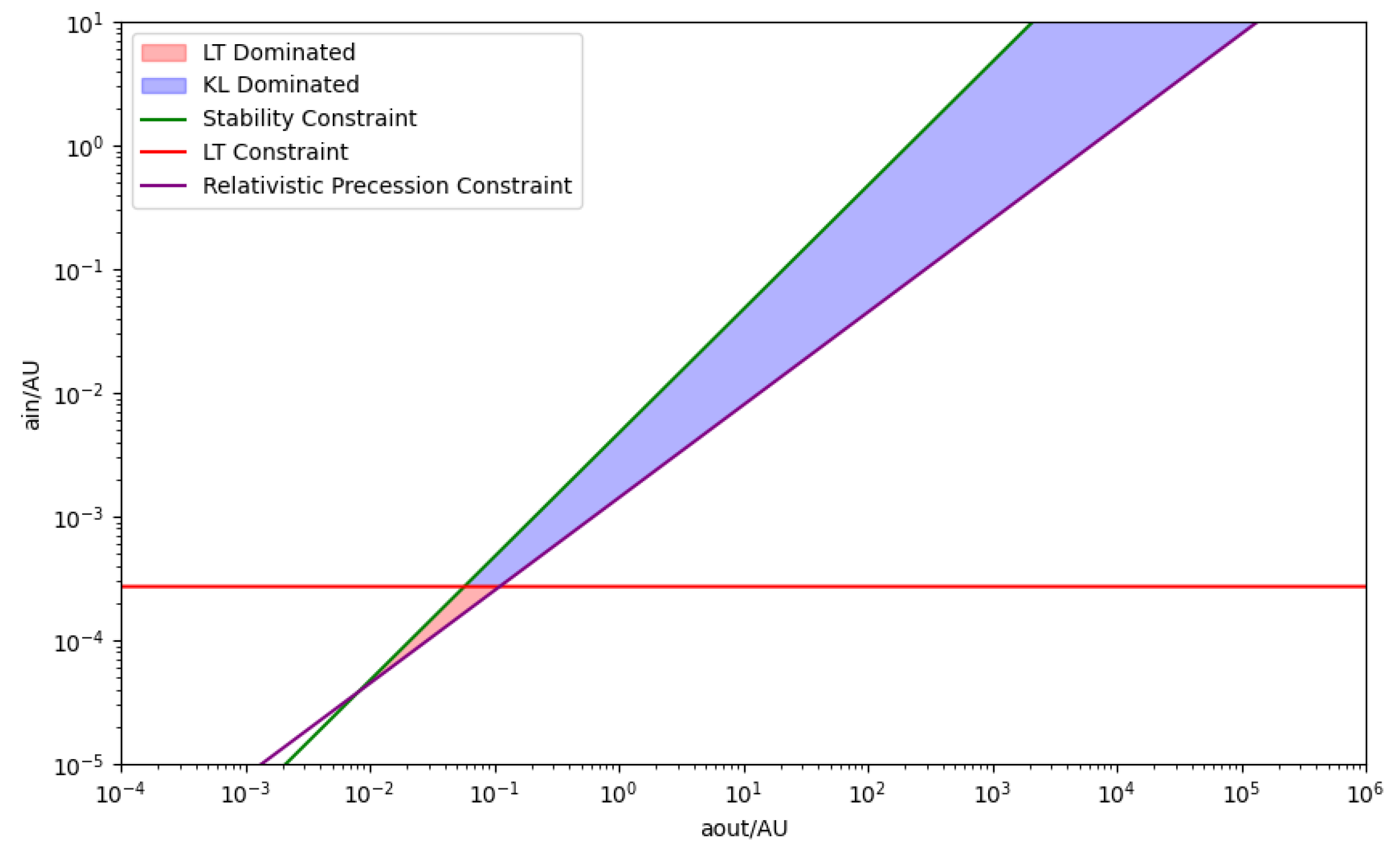
Figure 4.
Comparison of simulation results for intermediate models IM1, IM2, IM3, and SM5. Left column: Newt3 simulations. Right column: GR3 simulations.
Figure 4.
Comparison of simulation results for intermediate models IM1, IM2, IM3, and SM5. Left column: Newt3 simulations. Right column: GR3 simulations.
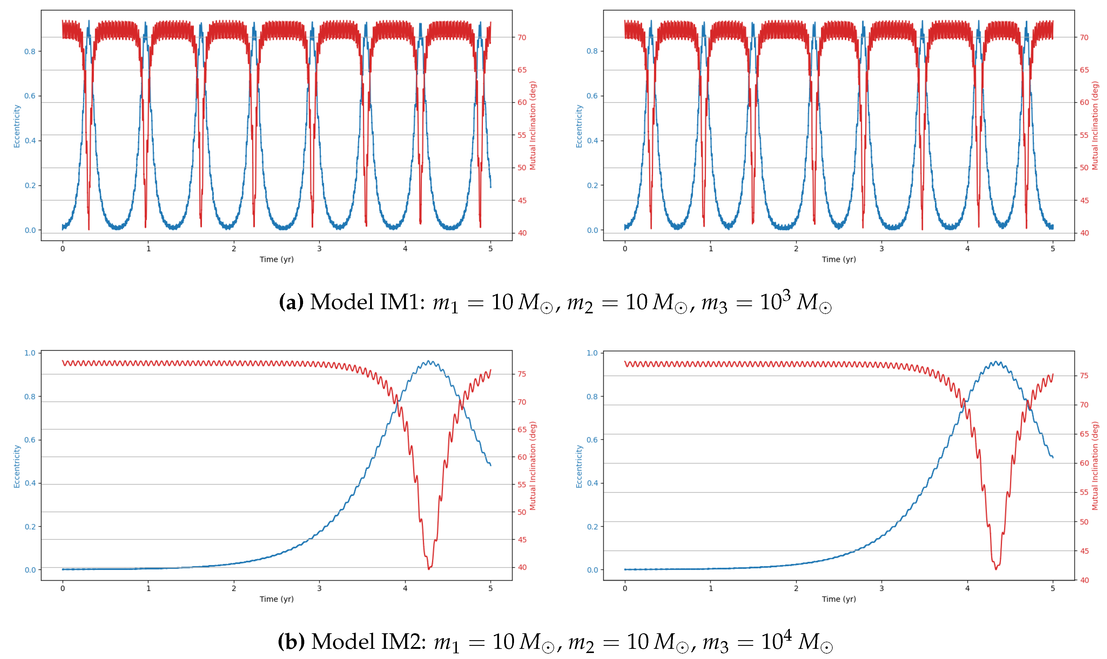
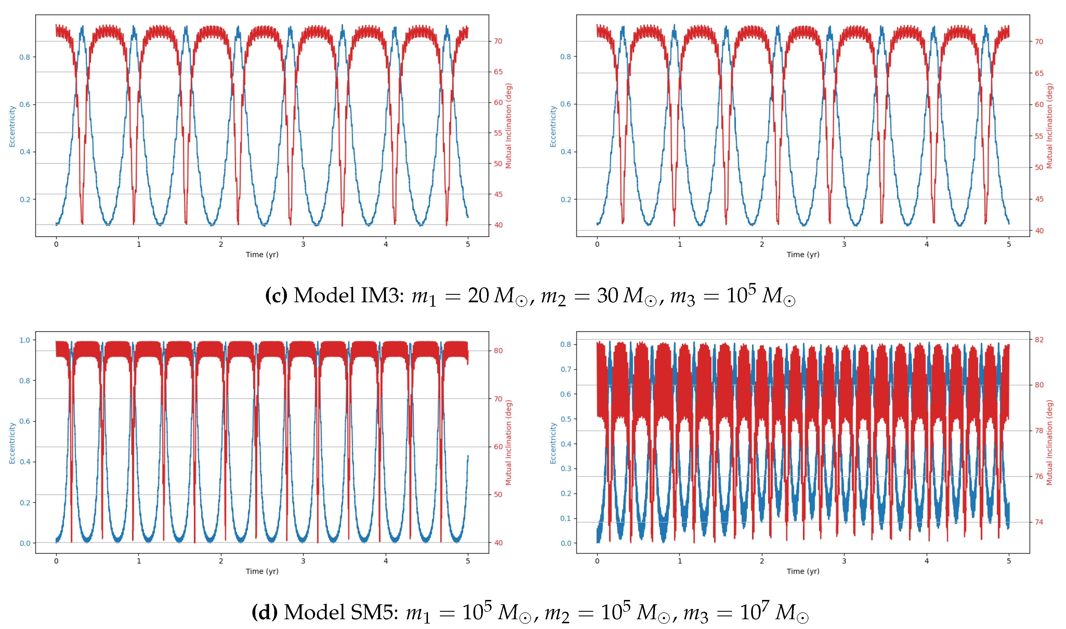
Figure 5.
Simulation results for models SM1, SM2, SM3, SM6, and SM7. Left column: Newt3 simulations. Right column: GR3 simulations.
Figure 5.
Simulation results for models SM1, SM2, SM3, SM6, and SM7. Left column: Newt3 simulations. Right column: GR3 simulations.
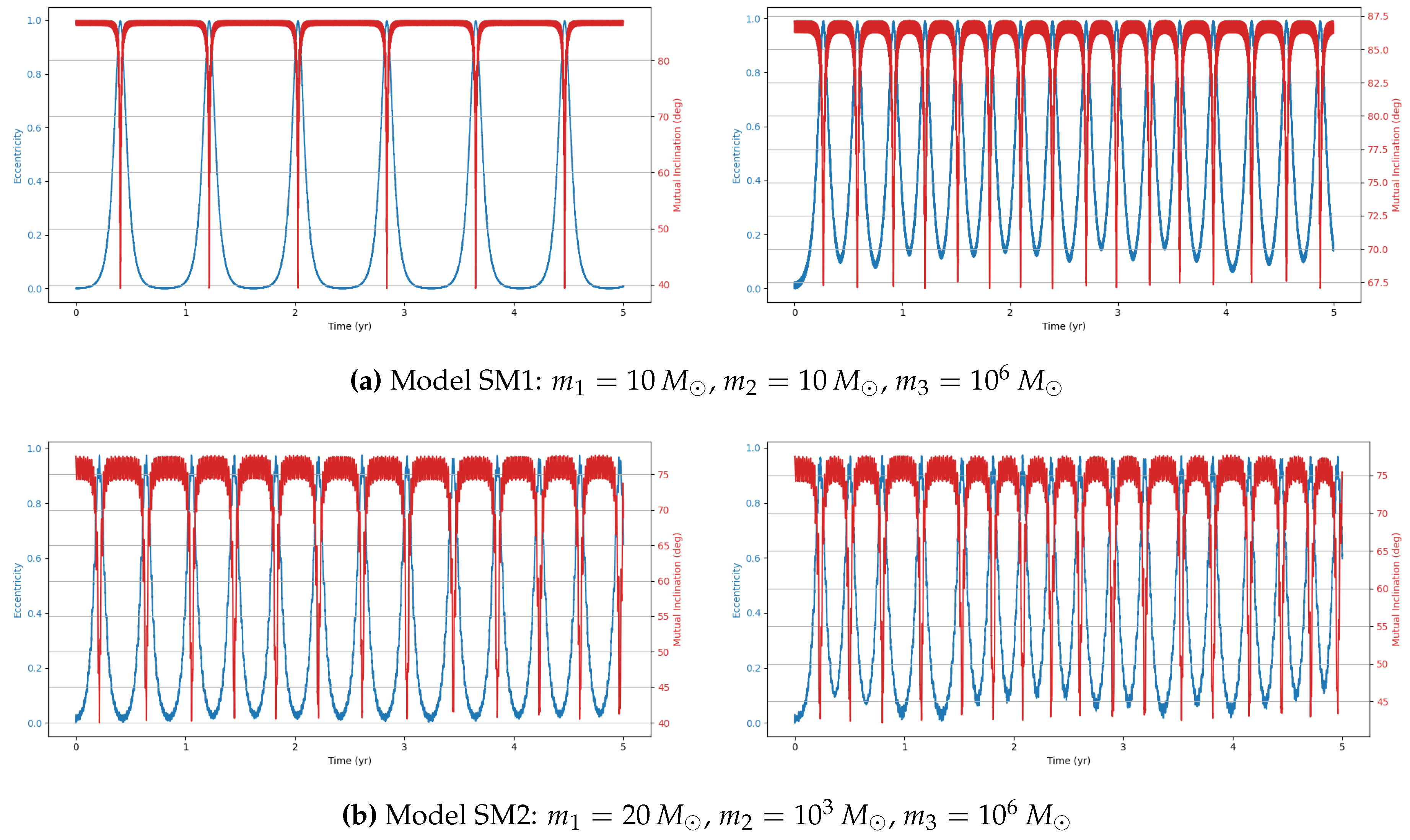
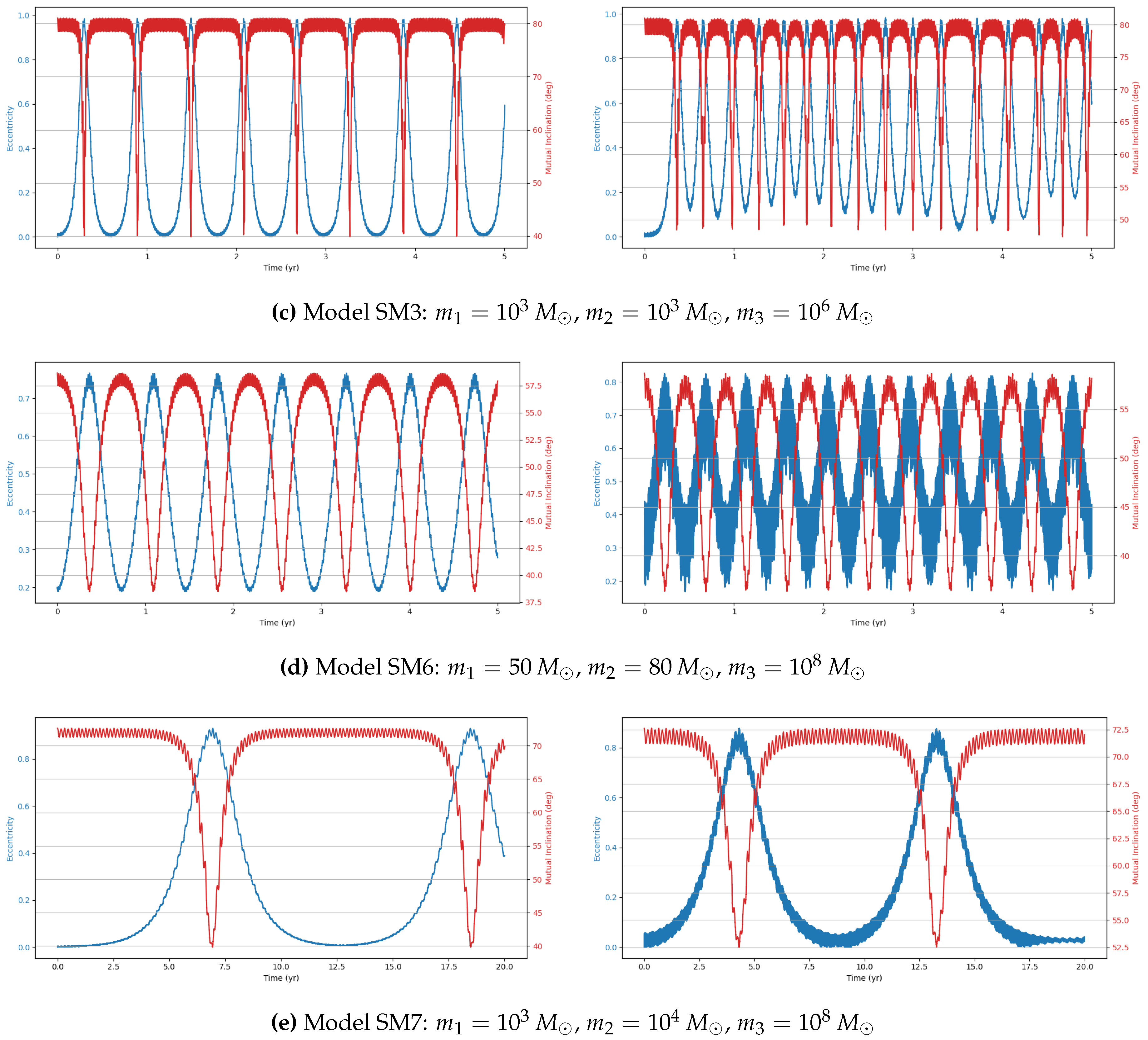
Figure 6.
Simulation results for model SM4 (, , ). Left: Newt3 simulation. Right: GR3 simulation.
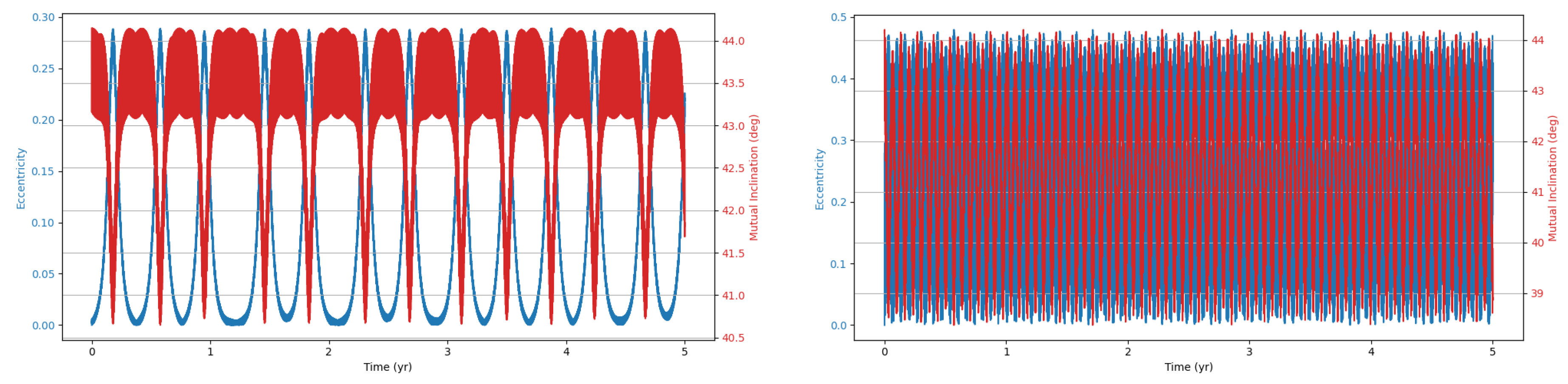
Figure 7.
Simulation results for model IM4 (, , ). Left column: Newt3 simulation results. Right column: GR3 simulation results.
Figure 7.
Simulation results for model IM4 (, , ). Left column: Newt3 simulation results. Right column: GR3 simulation results.
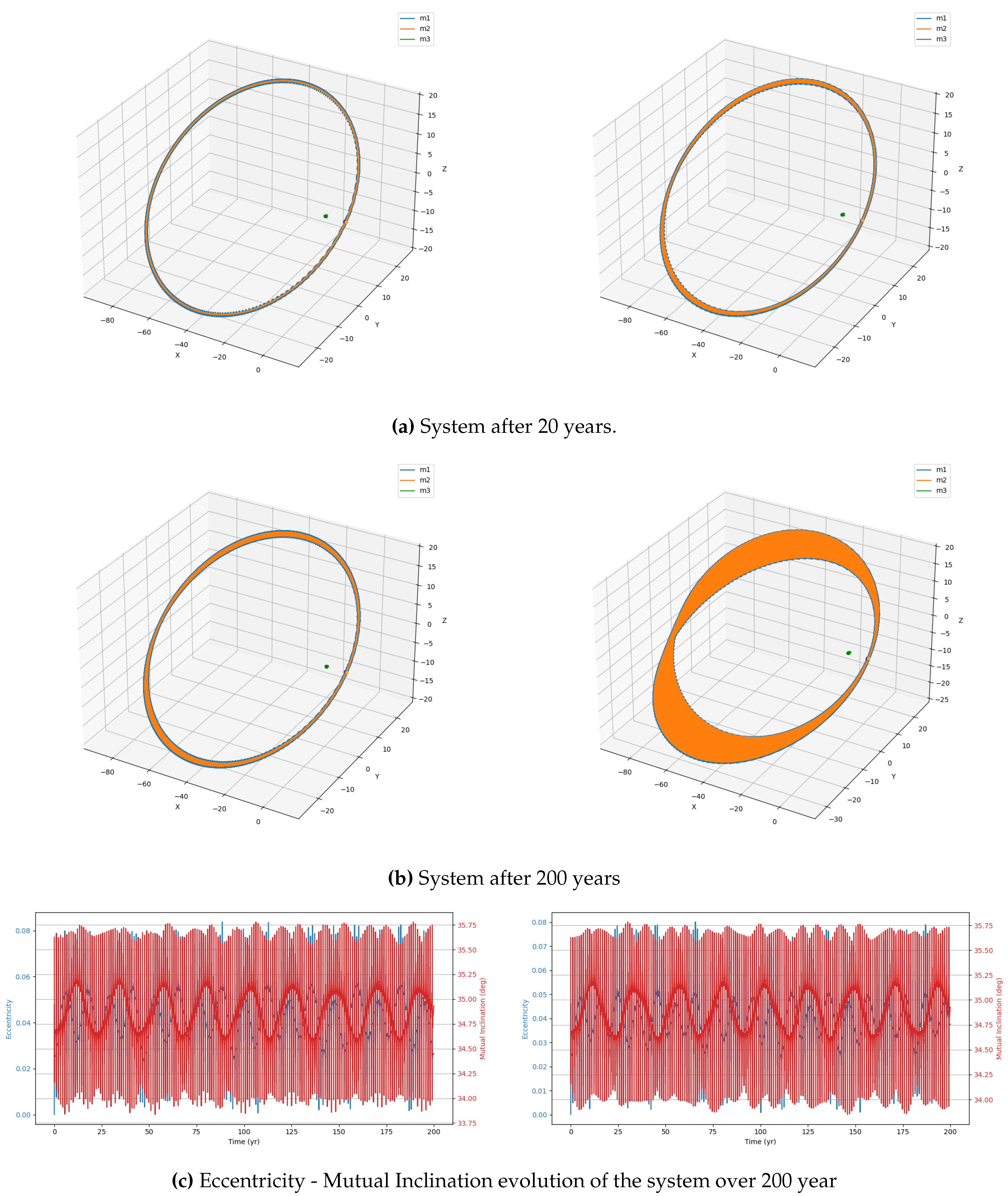
Figure 8.
Simulation results of systems IM5 and SM9 after 5 and 30 years respectively. Left column: Complete system. Right column: Inner binary.
Figure 8.
Simulation results of systems IM5 and SM9 after 5 and 30 years respectively. Left column: Complete system. Right column: Inner binary.
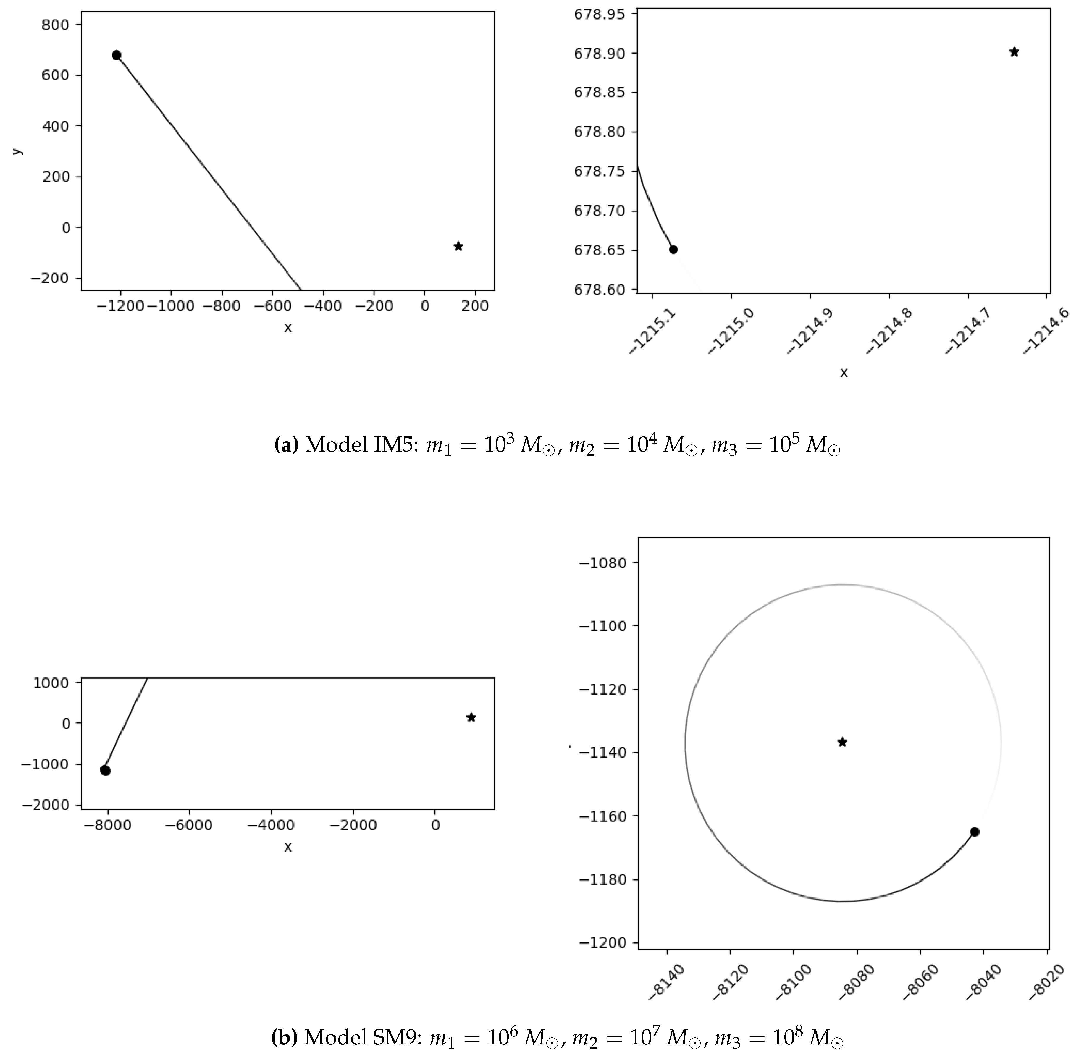
Figure 9.
Detectability of different binary mass combination from our models.
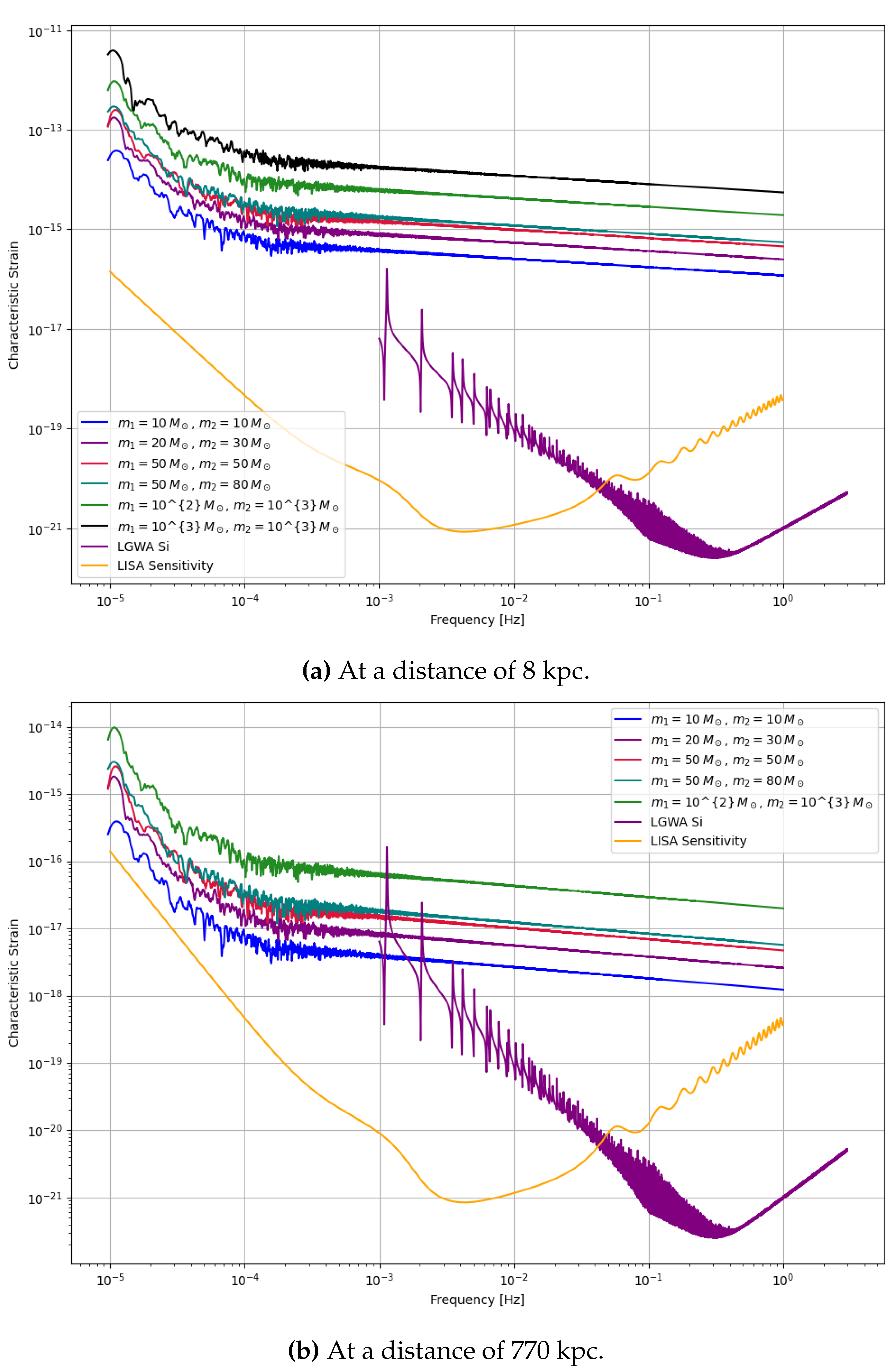
Figure 10.
Same binary at a distance of 770 kpc with different eccentricities.
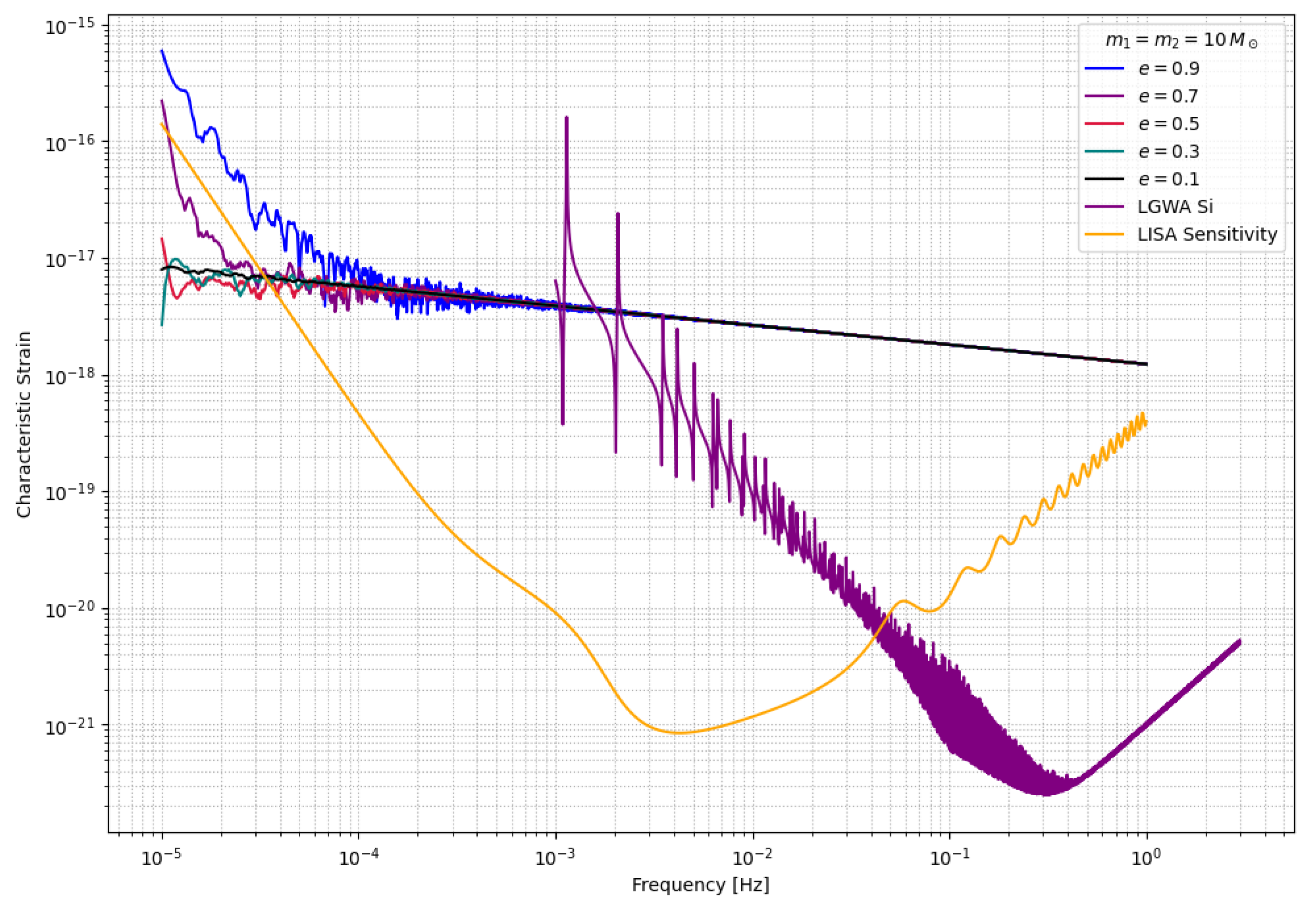
Figure 11.
Extending Detection Range thrugh multiple detectors
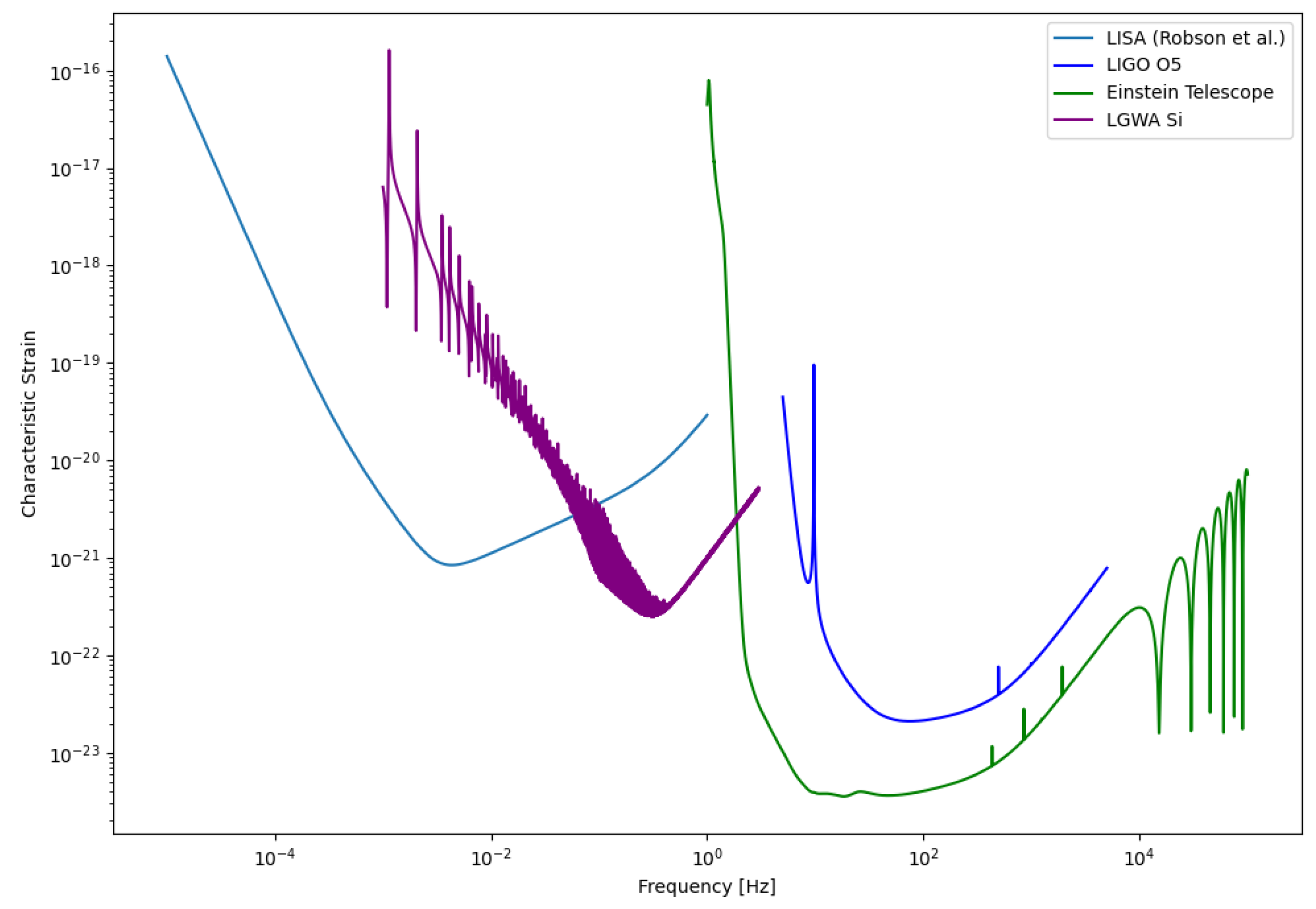

Table 1.
Models.
| Tertiary | Binary | Model | |||
|---|---|---|---|---|---|
| SBH - SBH | 10 | 10 | IM1 | ||
| SBH - SBH | 10 | 10 | IM2 | ||
| IMBH | SBH - SBH | 20 | 30 | IM3 | |
| SBH - IMBH | IM4 | ||||
| IMBH - IMBH | IM5 | ||||
| SBH - SBH | 10 | 10 | SM1 | ||
| SBH - IMBH | 20 | SM2 | |||
| IMBH - IMBH | SM3 | ||||
| SBH - SBH | 50 | 30 | SM4 | ||
| SMBH | IMBH - IMBH | SM5 | |||
| SBH - SBH | 50 | 80 | SM6 | ||
| IMBH - IMBH | SM7 | ||||
| IMBH - IMBH | SM8 | ||||
| SMBH - SMBH | SM9 |
Table 2.
Model Parameters.
| Model | I [Deg] | |||||||||
|---|---|---|---|---|---|---|---|---|---|---|
| IM1 | 10 | 10 | 1 | 0 | 0 | 90 | ||||
| IM2 | 10 | 10 | 5 | 0 | 0 | 90 | ||||
| IM3 | 20 | 30 | 5 | 80 | ||||||
| IM4 | 10 | 0 | 0 | 50 | ||||||
| IM5 | 10 | 0 | 0 | 100 | ||||||
| SM1 | 10 | 10 | 5 | 0 | 0 | 90 | ||||
| SM2 | 20 | 10 | 0 | 0 | 90 | |||||
| SM3 | 10 | 0 | 0 | 90 | ||||||
| SM4 | 50 | 30 | 5 | 0 | 45 | |||||
| SM5 | 1 | 20 | 0 | 0 | 100 | |||||
| SM6 | 50 | 80 | 50 | 0 | 60 | |||||
| SM7 | 1 | 200 | 0 | 0 | 80 | |||||
| SM8 | 1 | 150 | 0 | 0 | 70 | |||||
| SM9 | 50 | 500 | 0 | 0 | 90 |
Disclaimer/Publisher’s Note: The statements, opinions and data contained in all publications are solely those of the individual author(s) and contributor(s) and not of MDPI and/or the editor(s). MDPI and/or the editor(s) disclaim responsibility for any injury to people or property resulting from any ideas, methods, instructions or products referred to in the content. |
© 2026 by the authors. Licensee MDPI, Basel, Switzerland. This article is an open access article distributed under the terms and conditions of the Creative Commons Attribution (CC BY) license (http://creativecommons.org/licenses/by/4.0/).
Copyright: This open access article is published under a Creative Commons CC BY 4.0 license, which permit the free download, distribution, and reuse, provided that the author and preprint are cited in any reuse.


