
Submitted:
20 January 2026
Posted:
20 January 2026
You are already at the latest version
Abstract
A number of approaches to a theory of quantum gravity assume the fabric of spacetime is distinct from the spacetime of the material world of matter and energy. On a short time scale, one cannot distinguish between the fabric of spacetime expanding, nominally due to dark energy, or the scale of the material world contracting with respect to the fabric of spacetime. Contraction of the scale of the material world (length, time, mass, and charge contracting equally) maintains observable physical laws and results in a decreasing derived dark energy density matching that reported by the DESI Collaboration in March 2025. The DESI fits to the dark energy density over time show a distinct difference between those using scale-dependent supernovae data and those using mostly scale-independent angular measurements, such as from CMB and BAO measurements. That difference is resolved by applying a scale contraction rate of -3%/Gyr to the supernovae data. Scale contraction of the material world eliminates the need for dark energy to explain the apparent expansion of space, resolving the ~10122 discrepancy between the dark energy density required to match observation and that calculated for the vacuum energy as the mechanism for dark energy. The large force of the vacuum energy is a potential mechanism for compression of the material world, and would explain why the observed expansion only occurs outside of gravitationally bound systems. A scale-contraction model for cosmological kinematics explains why the dark energy density appears to be decreasing without requiring the underlying vacuum energy to be changing with time. Scale contraction of the material world predicts the observed directions and order of magnitude of the Hubble tension and the S8 tension, which has been a challenge to other proposed modifications of ΛCDM since those two tensions have opposite trends over time, the Hubble constant being about 10% larger in the late universe compared to the early universe, and the structure constant, S8, about 10% smaller. Scale contraction of the material world can be tested by modifying the LCDM cosmological model to include scale contraction over time, and assessing if the Hubble and S8 tensions are quantitatively reduced or resolved.
Keywords:
cosmology
; dark energy
; hubble tension
; DESI
; S8 tension
1. Introduction
The standard cosmological model, ΛCDM with a cosmological constant and flat spacetime, is increasingly recognized to be missing some cosmological physics [1,2,3,4,5]. This is due to discrepancies between model predictions and observations, such as parameter values varying depending on whether early or late universe data are used, and recent dark energy measurements. The Hubble tension is well known and statistically significant at the 5σ level [3]. The tension in the cosmological structure constant, S8, is less well known, but recent measurements have increased the statistical confidence in the discrepancy between S8 values for the early and late universe. Resolving the Hubble and S8 tensions simultaneously is a challenge to update ΛCDM since most proposed corrections affect those two parameters oppositely [3]. The recent DESI results on the dark energy density [6], supported by subsequent analysis taking into account the age-bias in the supernovae “standard candles” used in the dark energy measurements [7], show the dark energy density to be decreasing with time, in contrast to the assumed constant value in ΛCDM and the expected constant value if dark energy is due to the vacuum energy.
The possibility that the fabric of spacetime is a distinct entity from the spacetime of the material world (matter and energy) is suggested by John Wheeler’s summary of general relativity: “Matter tells spacetime how to curve, and curved spacetime tells matter how to move” [8], and that the mass-on-a rubber-sheet analogy attributes different properties to the fabric of spacetime (the rubber sheet stretching) and matter (movement with respect to the rubber sheet). More quantitatively, there are several approaches to a theory of quantum gravity that either explicitly or implicitly assume the fabric of spacetime is a distinct entity from the spacetime of the material world of matter and energy. [9,10,11,12,13,14,15]. That distinction motivates the consideration that the physical scale between the two spacetimes can change over time.
A positive cosmological constant leads to sufficiently distant galaxies moving apart at speeds exceeding the speed of light. Expanding space means the energy associated with a volume of space increases indefinitely with time, violating conservation of energy and raising the question of where that additional energy comes from. A scale contraction cosmological model can avoid violating these physical principles.
In Section 2 we show that the Hubble tension and S8 tension can be simultaneously resolved if a unit of time was larger in the early universe than it is now, setting a lower limit of scale decrease at 10%. In Section 3, we summarize the scale invariance of the equations of physics. In Section 4 we provide quantitative results showing consistency between the DESI measurements and the predictions from two models where the scale of the material world is decreasing with time. We find that a simple scale-invariant model for the apparent expansion of the universe predicts that the dark energy density will decrease with time. Section 5 briefly discusses other tensions resulting from the standard model and shows that those results can be explained by a contracting scale of the material world. The quantitative results consistently correspond to a scale decrease of the material world of about 35% since the Big Bang. Modification of the ΛCDM model to rigorously test the possibility of STM contraction as the missing physics in the standard cosmological model is discussed in Section 6. In section 7 we review a number of physics principles and cosmological considerations, and show that a contracting material world is consistent with those and resolves some of those concerns with the Λ/dark energy model for expansion of the universe. Section 8 provides a summary and conclusions from this work. The Appendix provides the equations and parameters used for the scale contraction models.
Hereafter, we refer to the spacetime of the material world as the STM, and the fabric of spacetime of the cosmos as the STF.
2. Bounds on and Estimate of Scale Change
The Hubble parameter is given by H(t) ≡ v(t) / r(t), where v is the recessional velocity of a distant object, and r is the distance to that object. For isotropic expansion of the universe, the recessional velocity is proportional to the distance of that object, so H(t) has the same value for all objects at a given distance (ignoring local motion). The Hubble parameter varies with time as the universe transitions between radiation-pressure driven expansion, gravitational contraction, and dark energy driven expansion. The Hubble constant is the current value of the Hubble parameter, H0 = H(t = now). The value of the Hubble constant can be derived from cosmological data at various times by measuring the Hubble parameter and using the cosmological model to propagate that value to the current time. The Hubble constant is about 10% lower when determined from the early universe phenomena of the cosmic microwave background (CMB) and baryon acoustic oscillations (BAO) (~67 km/s/Mpc), compared to measurements of the Hubble constant from late universe supernovae (~73 km/s/Mpc) [2]. The Hubble parameter has units of inverse time, so a scale change where a unit of time was 10% larger in the early universe would resolve the Hubble tension. Extrapolation from the early universe Hubble parameter to the current Hubble constant uses the cosmological model, so the 10% scale change is a lower limit since ΛCDM is tuned to match cosmological data at all times, and will be partially compensating for any scale change affects in the early universe data.
Cosmic shear measures the “clumpiness” of the universe. The CMB shows the early universe to be highly uniform. Gravitational attraction causes matter to clump into stars, galaxies, and galactic clusters. The amount of that clumping is represented by a statistical quantity, S8, which measures the amplitude of matter density fluctuations in the late universe. The ΛCDM model is used to extrapolate CMB measurements to the current era. Weak gravitational lensing of galaxies at various redshifts and other techniques are used to measure the current value of S8. The early and late universe measurements are consistent within themselves, but disagree with each other, although that difference at the 2-3 σ level is less statistically significant than the 5σ Hubble tension [3,16]. Values for S8 estimated from late universe data (S8 = ~0.75) are about 10% lower than those extrapolated from CMB data (S8 = ~0.83) [3]. While S8 is a dimensionless number, it is expected to increase with time as gravitational clumping occurs. It has been measured to increase approximately linearly with time when measured with low-z data [3]. That time dependence means S8 should decrease with time as the scale factor decreased. Again, that 10% difference is expected to be a lower limit on the scale change due to tuning of the ΛCDM model. The observation that both the Hubble tension and the S8 tension are simultaneously resolved by a 10% (or more) decrease in scale factor over time is a strong reason to consider scale change as physics to be added to the ΛCDM model, given the difficulty other proposed revisions of ΛCDM have in simultaneously resolving both those tensions.
The measurements that led to the conclusion the universe is expanding rather than contracting were measurements of “standard candle” Type Ia supernovae (SN Ia). Measurements of the high-z SN Ia showed those SN were much dimmer than expected, which led to the conclusion that the universe was expanding. Depending on the method used to measure actual distances, the galaxies at z=1 were ~0.25 to ~0.33 magnitude fainter than expected ([17] Figures 4 and 5, data fit curve at z=1), or ~0.029 ± 0.004 mag/Gyr.
SN at z = 1 emitted their light about 7.7 Gyr before present. The scale factor would have been larger then, so an interval of time would have been larger. Since the number of photons does not change with scale factor, the number of photons/sec received will decrease as an interval of time gets smaller. While the detector size and distance to the SN will also decrease with decreasing scale, the detector is measuring the flux in a certain solid angle from the source, which will not change with scale factor since solid angle is scale invariant. Converting the dimmer magnitude to a fractional decrease in scale gives a fractional scale reduction of –0.026 ± 0.004 /Gyr. This gives an estimate of 0.64 ± 0.05 for the current scale factor relative to that at the Big Bang, assuming an age of 13.8 Gyr for the universe and a constant rate of change in the scale.
The DESI BAO data [6] can be used to estimate the current amount of scale change since the Big Bang. Figure 1 of [6] shows how the DESI BAO data constrain the expansion history of the Universe, with the BAO size across the line of sight (LOS), α⊥, constraining the distance from us, and the BAO size along the LOS, α||, constraining the expansion rate and the slope of the fit to the data in the Figure. That Figure shows the ΛCDM prediction for non-zero constant dark energy and the ΛCDM prediction with no dark energy. The DESI BAO data lie on the former. The Figure plots the relative size of the universe against the age of the universe. The α⊥ data will not be affected by scale contraction since they are angular data, but the α|| data will. Since the slope is inversely proportional to α||, smaller α|| due to scale contraction will result in a larger slope compared to the zero-dark-energy prediction. The slope for the dark energy curve is 0.68/Gyr and the slope for the zero-dark-energy curve is 0.45/Gyr, consistent with scale contraction and giving a current scale factor of 0.66 (=0.45/0.68) relative to a scale factor of 1.00 at the Big Bang. The data are analyzed in more detail in Section 5, showing that the DESI BAO data are consistent with scale contraction over time for the baseline scale contraction model.
The Hubble and S8 tensions are not resolved by the current cosmological model and their opposite directions with respect to time are a challenge for an alternative cosmological model. Scale contraction resolves both tensions in the needed direction, and imposes a minimum scale contraction of 10% since the big Bang. The relative faintness of high-z SN Ia gives a current scale factor of ~0.64 ± 0.05 relative to the Big Bang, and the DESI BAO data give a consistent value of 0.66 for the current scale factor, and the resulting ~35% scale contraction is consistent with the limits set by the Hubble and S8 tensions. While the latter two calculations are not as compelling an argument for scale contraction as the simultaneous resolution of the Hubble and S8 tensions, the consistency of the resulting scale factor points to an underlying common feature of the universe.
3. Scale Invariance
Scale invariance describes several phenomena in physics. Here we use the term “scale invariance” to mean the situation where the mathematical laws of physics do not change when the scale of the material world changes. Specifically, when the scale of the measurables of the physical world (mass, length, time and charge; M, L, T, Q) change in unison, the physical laws do not change.
For cosmological dynamics, force and the gravitational constant are scale independent with respect to uniform scaling of the measurable quantities. Force has units of ML/T2 which does not change under that scale change. Similarly, the gravitational constant G does not change since F=Gm1m2/r2 is also scale invariant, as is the speed of light, c = L/T. Since gravity is the dominant force for cosmological dynamics on “short” time scales (dark energy currently expands space at a rate of ~3%/Gyr versus ~7%/yr overall expansion rate [18]), scale change in the material world will only show cosmological affects at time scales greater than about one Gyr. The main sources of cosmological information, photons and gravity waves, both travel at the speed of light, so are not directly useful to probe scale change. On “short” time scales (<<1 Gyr), cosmological dynamics cannot resolve whether scale change is occurring or not.
There is a nuance here in applying scale invariance. The electromagnetic field without charged particles is scale invariant. Quantum electrodynamics (QED) includes charged particles, and is consistent with both quantum mechanics and special relativity, but is traditionally not considered to be scale invariant since the electric charge and system energy scale together [19,20]. We are concerned here with what is physically measurable. Energy has units of ML2/T2, which has a linear dependence on scale factor, and would then be expected to scale with electric charge as seen in QED. This illustrates that it is important to distinguish between measurements of quantities (potentially including physical constants) from within the scaled system, and from an unchanging reference outside that system. For example, G and Coulomb’s constant k (ML3T-2Q-2) are scale invariant in this context, whereas Planck’s constant h (ML2/T) is not. Since one cannot directly detect scale change within the system, Planck’s constant would appear to be constant, whereas outside the changing system, measured in unchanging units, Planck’s constant would appear to be changing.
Until the recent DESI results [6], the cosmological constant (and dark energy as a physical mechanism for that term in Einstein’s field equations) was assumed to be constant. Assuming dark energy is a constant pressure term, the force from dark energy will be proportional to the area of the region subject to that pressure. With a decreasing scale term for the material world, that area will decrease with time, resulting in a reduced force over time. We noted above that cosmological dynamics from gravity are invariant under scale change, so this model predicts that the force from dark energy will decrease with time with respect to gravitational forces if the material world has a decreasing scale factor. A decreasing scale factor for the material world resolves how the pressure of dark energy can be constant at the same time as the acceleration from dark energy is decreasing, as seen in the DESI results.
The standard model of particle physics is consistent with what is expected if the material world is able to change scale. The model does not predict specific particle masses directly. It has 19 input parameters [21], some of which are needed to match the observed particle masses. This suggests the particle masses may not be fundamental quantities in the theory since measurement is required to determine a scale factor for them.
4. Quantitative Comparison to the Desi and Other Results
The March 2025 DESI fits to the dark energy density over time contain two important aspects that can be explained with a contracting scale factor for the STM. First is that a scale contraction model quantitatively reproduces the apparent dark energy decrease in the late universe, and second is to show that STM scale contraction resolves the variation in fit results between the different data sets used.
Different types of data are affected differently by scale change. Angular measurements, such as CMB data, are not affected by scale change since an object twice the distance and twice the width as a reference object will have the same angular size. Baryon Acoustic Oscillations (BAO) data will have scale dependence when measured along the line-of-sight (LOS) since that is a distance measurement. BAO measured perpendicular to the LOS are angular measurements and scale invariant. The supernovae data here are scale-dependent since they typically use “standard candle” supernovae and combine luminosity with (scale-dependent) redshift to infer a distance to the object.
4.1. Scale Contraction Models Predict a Decreasing Dark Energy Density Matching the DESI Results
Henderson has developed a late-universe model for scale contraction (SC) of the STM [18]. There are two steps in developing the SC model. First is to derive a reference model for universe expansion due to dark energy. To permit comparison to the DESI results, the parameter for the dark energy (DE) density in the DE reference model (the model representing expansion due to dark energy) is tuned via least squares analysis to match the Hubble parameter over time for the ΛCDM model used in the DESI analysis. Since the DE reference model does not include a radiation term or gravitational contraction, it is only valid in the late universe where dark energy is the dominant term for cosmological dynamics. The second step is to develop one or more SC models. The SC models can be analytically anchored to the reference model by matching the current cosmic scale parameter and expansion velocity. The SC models then provide a prediction of the late universe apparent dark energy density that can be compared to the DESI results.
The baseline SC model, EXP, assumes the STM scale factor decreases exponentially over time, with time measured in the unchanging STF system. The rationale for this was the assumption that the mechanism driving the contraction would become less effective as contraction proceeded. This is a standard relaxation model for a system out of equilibrium. If one considers the Big Bang to be a non-equilibrium event, exponential relaxation back to the zero-energy state presumably preceding the Big Bang is physically reasonable. EXP has no fit parameters, using a parameter related to the dark energy density that was derived for the DE reference model.
The vacuum energy provides a force ~10122 times larger [22,23] than the force required for the expansion of space attributed to dark energy. That large a force is plausible as a mechanism driving contraction of the STM. Analogous to the Casimir force, the smaller value of the vacuum energy within a galactic structure due to truncation of the allowed quantum modes means there would be an external pressure on those structures. This extra-galactic pressure potentially is the explanation for why dark energy only acts outside gravitationally bound systems – the contraction of the gravitationally bound system being seen as expansion of the extra-galactic medium when viewed from the STM. Henderson modeled how a constant vacuum energy pressure would act on a region of the material world [18] and found it generated exponentially decaying contraction of the STM [18], consistent with the vacuum energy as a plausible mechanism causing contraction of the STM.
Other SC models were tested, such as the scale factor decreasing linearly in either STF time or STM time.
A linear decrease of the scale factor with STF time exactly reproduces the DE reference model. Physically, this means that the kinematics of a universe expanding due to time-invariant dark energy are the same as the kinematics of a universe where the STF is unchanging and the STM is contracting linearly in STF time. While the material world has a finite time in STF units before the scale factor goes to zero, it takes an infinite amount of STM time for the scale factor to go to zero, since an interval of STM time is contracting with respect to an interval of STF time.
A linear decrease of the scale factor with STM time resulted in an apparent dark energy density that was increasing with time, which is the opposite of what was seen in the DESI results. That SC model is not considered further here.
A generic model was developed to allow for a parametric fit to the data to constrain an SC model. For example, if the vacuum energy is causing contraction of the STM, as that contraction proceeds, the apparent (STM) distance between galactic clusters will increase, so the compressive force due to the vacuum energy (VE) will increase also. This can be modeled by increasing the value of the fit parameter n from n = 2 for the exponential decay model, to n > 2, which models the contraction force becoming relatively stronger with time. Here we use a value of n = 2.5 to illustrate the utility of a generic model, clearly show the differences between the EXP and VE models, and to anchor discussion of testing SC as the potential missing physics in ΛCDM.
The formulae and fit parameters for the DE and SC models are given in the Appendix.
Figure 1 shows a comparison of the relative (normalized to its current value) dark energy density for the DESI fits for several data sets, and three scale contraction models. Note that the DESI BAO + CMB results are notably different than the three DESI fits which include SN data. The EXP scale contraction model is the exponential decay model tuned to the ΛCDM model for a cosmological scale parameter over the range of a = 0.8 to 1.0. The VE model is similar, but with an approximate correction for the relative increase of the vacuum energy force as the STM contracts. The EXP-Mixed model is similar to the EXP model, but tuned to include more of the early universe, with a cosmological scale parameter over the range of a = 0.6 to 1.0, which means it will include more of a mix of scale-independent data such as from the CMB, and scale-dependent late universe data such as from SN. Including more of the early universe in the SC model lowers the slope of the relative dark energy density, in accord with the DESI fits having a lower slope when SN data are included. The SC models lie within the envelope of the DESI fits, which is to be expected since they are matched to the ΛCDM model, and the ΛCDM model has been tuned to fit CMB, BAO, and SN data.
Section 4.3 shows that all of the DESI fits using SN data align better with the BAO + CMB fit when a scale correction has been applied to the SN data, showing that neglecting a scale correction for scale-dependent data lowers the apparent dark energy density, as seen in the fits to the SN data in Figure 1. The EXP-Mixed (a = 0.6 to 1.0) fit is lower than the EXP fit, since it includes more of the early universe kinematics, but the slope is a better match to the DESI fits at earlier times, consistent with the ΛCDM model including that early-time data. The VE model shows the best agreement with the BAO + CMB fit (and the scale-corrected SN fits in Figure 2), in agreement with the physical expectation that a compressive force from the vacuum energy will become relatively stronger over time as the apparent distance (i.e., measured in STF units) between galactic clusters increases.
Figure 1.
Dark energy density over time from fits to the DESI DR2 data (lines without symbols) ([6], Table V] and predicted from the SC models (lines with symbols). All the data shown are normalized to a value of 1 at the current time to facilitate comparison between them, and to focus on the current rate of change of the apparent dark energy density. The DESI BAO + CMB data are largely scale invariant, with only a small scale-dependent contribution from the BAO|| LOS data. The other three DESI fits (dashed lines with no symbols) include supernovae data, which are scale dependent and are clearly clustered away from the DESI BAO + CMB fit (solid line with no symbols). The baseline SC model is the EXP model, which models the scale contraction as exponentially decreasing per a system relaxing back to its initial state. The EXP model lies in the middle of the DESI fits. The EXP model is tuned to the late universe (cosmological size parameter a = 0.8 to1.0) and shows a decreasing apparent dark energy density matching that of the aggregate DESI fits. The EXP-Mixed model includes a larger time span (a = 0.6 to 1.0) and will therefore have more of a mix of early (large scale change) and late (small scale change) universe data from the ΛCDM model, and consequently fits the three mixed-scale DESI supernovae fits better than the EXP model. The VE model assumes the relative strength of the physical mechanism causing scale contraction is slowly increasing over time, as would be the case for the vacuum energy as discussed in the text. The VE model is the best fit to the current rate of change for the DESI DR2 dark energy density fits.
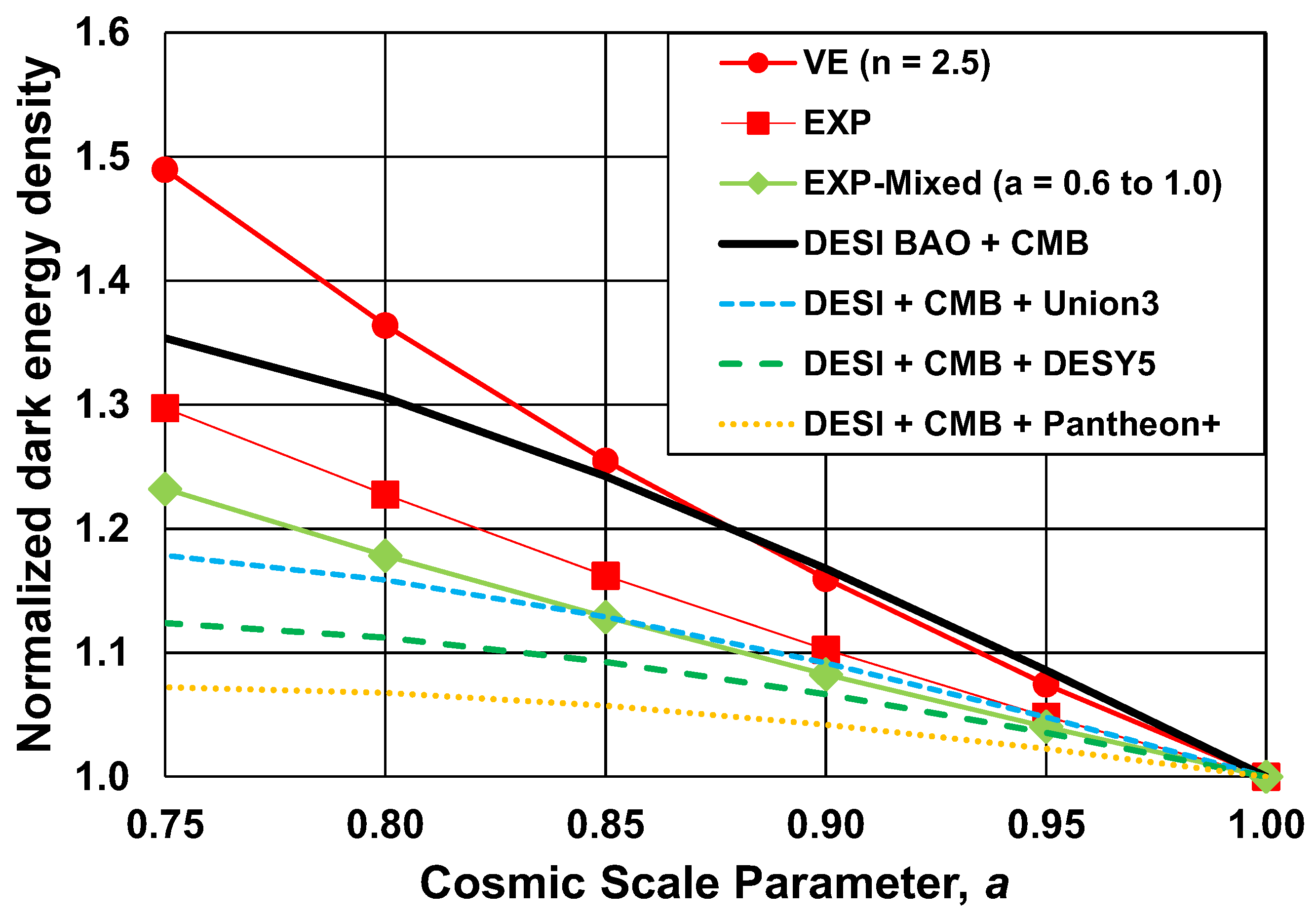
Figure 2.
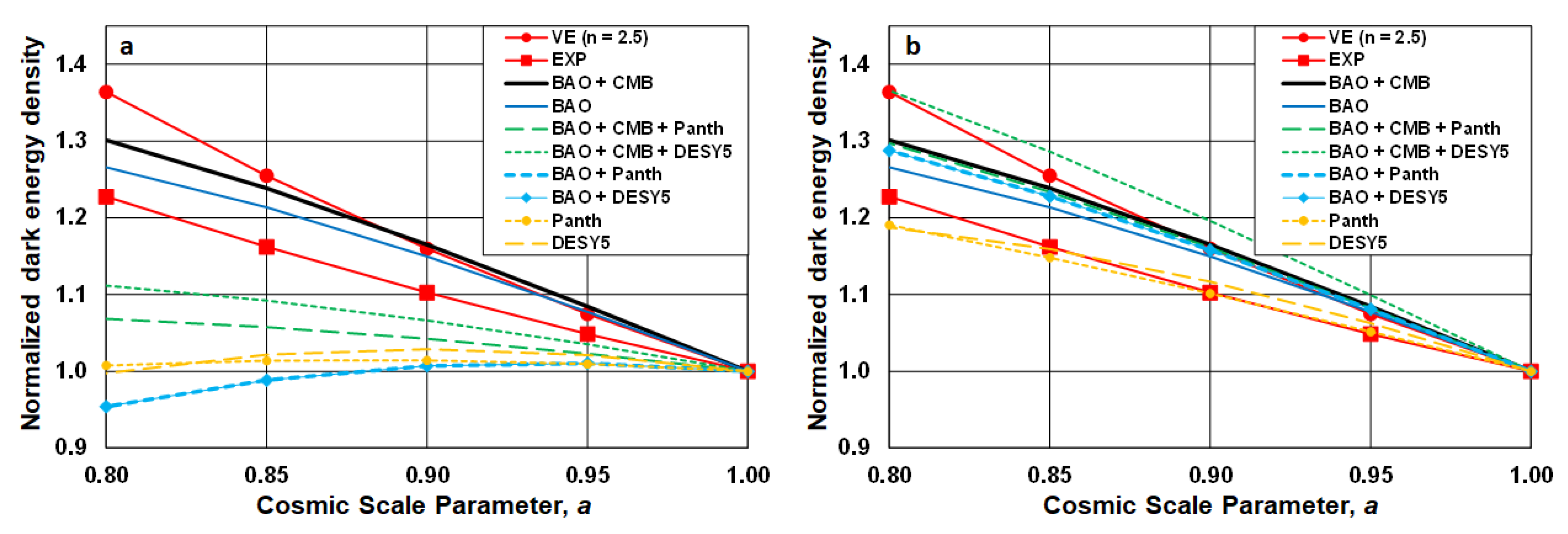
Comparison of the Son et al fits [7] to the DESI DR2 data (lines without symbols) and to the SC EXP and VE fits (red lines with symbols), before (left) and after (right) correction for age-bias and scale contraction of the SN data (dashed lines). The DESI BAO + CMB and BAO fits have no scale correction because they contain no SN data. The BAO data contain both scale independent (BAO⊥ angular data) and scale dependent (BAO|| LOS data). The CMB data are scale-independent angular data, hence reduce the impact of scale change in the BAO + CMB fit, which is why the BAO + CMB fit lies above the BAO fit. Scale correction of the SN data brings three of the six fits using SN data into agreement with the least scale-dependent BAO + CMB fit. The other three fits using SN data have their variation from the BAO + CMB fit greatly reduced with scale correction. The VE model now best describes the DESI results. The EXP model is tuned to the current ΛCDM model which includes SN data, so is expected to lie below the BAO + CMB fit as seen here.
Figure 2.
Comparison of the Son et al fits [7] to the DESI DR2 data (lines without symbols) and to the SC EXP and VE fits (red lines with symbols), before (left) and after (right) correction for age-bias and scale contraction of the SN data (dashed lines). The DESI BAO + CMB and BAO fits have no scale correction because they contain no SN data. The BAO data contain both scale independent (BAO⊥ angular data) and scale dependent (BAO|| LOS data). The CMB data are scale-independent angular data, hence reduce the impact of scale change in the BAO + CMB fit, which is why the BAO + CMB fit lies above the BAO fit. Scale correction of the SN data brings three of the six fits using SN data into agreement with the least scale-dependent BAO + CMB fit. The other three fits using SN data have their variation from the BAO + CMB fit greatly reduced with scale correction. The VE model now best describes the DESI results. The EXP model is tuned to the current ΛCDM model which includes SN data, so is expected to lie below the BAO + CMB fit as seen here.
4.2. Scale Contraction Models Predict the Observed Reduction in Supernova Brightness
As noted in Section 2, the measurements that led to the conclusion the universe is expanding rather than contracting were measurements of “standard candle” SN Ia. Depending on the method used to measure actual distances, the galaxies at z = 1 were ~0.25 to 0.30 magnitude fainter than expected [17], which is equivalent to 21% to 25% fainter. The EXP model for a = 0.6 to 1.0 predicts SN at z = 1 will be 21% dimmer than otherwise expected, and the VE model predicts they would be 22% dimmer (using scale factors from Section 5.2), consistent with those original measurements [17].
Subsequent SN Ia measurements and analysis have refined the correlation between SN age and brightness. Section 4.3 shows that the SC model matches those corrections, and that correcting the SN data used in the DESI fits results in a consistent set of fits for the evolving dark energy density.
4.3. Correction for Scale Contraction Restores Consistency to the DESI Fits
Figure 1 shows that the DESI DR2 fits for the dark energy density are notably different for the data sets that included SN data than for those that were largely free of scale dependent data, such as the BAO + CMB fit. The SN data are based on “standard candle” SN Ia having a known intensity which can be used with redshift to provide a measurement of the universe’s expansion history.
Recent work has shown that there is an age bias in that data at the 5.5σ level, which is generally not properly accounted for when using that data [24]. An age correction factor for that bias has been applied to the DESI DR2 BAO data [7]. The results confirm the DESI conclusion that the dark energy density is varying with time, but now at a higher (>9σ) level of significance. Chung et al [24] speculate on possible mechanisms for the observed age bias, but do not offer any firm conclusion.
Table 1 shows the dark energy density fits to the DESI data analyzed by Son et al ([7], Table 2), initial fits and fits corrected for SN progenitor age-bias, reformatted to highlight how the data are systematically affected by the amount of scale-dependent data used in the fit. The SC models can be used to estimate how much correction of the SN data is needed for the SN data to be consistent with the scale-independent CMB data. Section 2 showed that the observed SN light intensity decreases with a decreasing scale factor. For a = 0.8 to 1.0 the EXP and VE models give the relative scale factor decreasing at a rate of –3.4%/Gyr. For a = 0.6 to 1.0 the EXP model gives the relative scale factor decreasing at a rate of –2.7%/Gyr, and the VE model gives a rate of –2.8%/Gyr. This corresponds to a decreasing SN magnitude of –0.038/Gyr (= –2.5 log10(1/0.966) ), –0.030/Gyr, and –0.031/Gyr, respectively. The desired correction of the SN magnitudes is then approximately –0.034 ± 0.004 mag/Gyr due to scale change. Son et al [7] used a correction factor of –0.030 ± 0.004 mag/Gyr for the age-bias correction used in Table 1 and Figure 2b. Since this is the same as the desired correction due to scale change, within the uncertainty of each, those results can be taken as testing the validity of correcting for scale change to bring the DESI fits into consistency with each other. The last two columns of Table 1, and the curves in Figure 2b show that scale correction resolves the inconsistency of fits between data sets using the DESI data, supporting the validity of scale change as a mechanism to explain the apparent expansion of the universe and providing a potential explanation for why there is an age-bias in the SN data.
Son et al see the same result for the cosmological parameters Ωm (fraction of matter and dark matter in the universe) and q0 (present-day deceleration parameter) ( [7] Table 2), with those parameters for all data fits being more consistent with the BAO + CMB fit after the same age-bias correction has been applied. This shows that scale correction is relevant to a wider range of cosmological parameters than just those associated with dark energy.
The Chung et al results [24] provide even more detailed support of an SC cosmological model. For the SN data with z < 0.2 (the Rose+19 data set), they get an age-bias correction of –0.038 ± 0.007 mag/Gyr.
z = 0.2 corresponds to 2.40 Gyr before present in the SC models, or a range of a = 0.83 to 1.00. The corresponding correction from the SC models (for a = 0.80 to 1.00) was –0.038 mag/Gyr, identical to that derived from the SN data. For the SN data with z < 0.45 (the Gupta+11 data set), Chung et al get an age-bias correction of –0.025 ± 0.006 mag/Gyr. z = 0.45 corresponds to 4.65 Gyr before present in the SC models, or a range of a = 0.68 to 1.00. The a = 0.60 to 1.00 correction from the SC models was –0.030 mag/Gyr for the EXP model and –0.031 mag/Gyr for the VE model, consistent with the Chung et al results for the SN data with z < 0.45. The observation that the age-bias correction factor depends on the z-range of the SN data set in the Chung et al results, and that the SC models predict similar scale-correction values for those same z ranges supports scale change as the underlying mechanism for the observed age bias in the SN data.
Figure 2 plots the dark energy density for the fit parameters in Table 1, as well as the EXP and VE SC models. The 8 fits in Figure 2a make clear the trend that the more dependent the fits are on scale-dependent data, the lower the curve is. The BAO only fit also shows this trend since there is no CMB data to dilute the scale dependence of the along-LOS BAO‖ data. Correcting for scale dependence brings 3 of the fits using SN data into agreement with the BAO + CMB fit, and greatly reduces the fit discrepancy for the other 3 fits using SN data. The observation that the age-bias correction is z-dependent in both the Chung et al results and from the SC models suggests that using a scale correction tailored to each individual SN might further reduce the fit discrepancy for those 3 fits that do not overlap the BAO + CMB fit results.
The two SC curves in Figure 2a bracket the BAO + CMB and BAO fits, which have minimal scale-dependence, and are notably different from the six fits using SN data. In Figure 2b, three of the SN fits now lie between the BAO + CMB and BAO fits, and the VE model is clearly the best match to those five fits, particularly in the late universe (a > 0.9) where the SC models are most valid. This is consistent with the vacuum energy being the mechanism that drives scale contraction of the STM. However, both the EXP and the VE models are tuned to the current ΛCDM model which does not contain any scale correction. The results of Son et al show that correction of the SN data for age-bias or scale change moves those curves upwards, in which case an EXP model tuned to scale-corrected SN data could well match the BAO + CMB fit and the VE model would have a smaller value of the parameter that adjusts for the increasing pressure from the vacuum energy as the scale of the STM decreases.
4.4. Model Constraints from the DESI Results
The 2025 DESI results raise the question of what mechanism could cause the dark energy term in a cosmological model to change over time. Assuming the amount of matter is constant and the universe has had a flat geometry over time, the dark energy term will have started small, peaked 4 to 5 billion years ago (see Figure 3), and is now decreasing. There is no accepted model for this time-dependent behavior. The vacuum energy pressure is expected to be constant and either resulting in a dark energy density of zero or 10122 larger than the observationally-determined value, as discussed in Section 7.3. The DESI Collaboration has performed an exhaustive analysis of the DESI data compared to physical models, parametric models, and binning methods to analyze the data [25]. Three findings from that work are relevant here. First, that the data only support a two-parameter model; second, that the wowaCDM model is a good representative of the best fits to the data; and third, that all of the fits to the data show a region where w(z) < –1 (called a phantom crossing), violating the null energy condition of general relativity. That last finding is of particular concern since it would have “profound implications for fundamental physics,” requiring “exotic physics” for dark energy [25]. Several models were identified that avoided a phantom crossing, however those models had concerns about the required number and fine tuning of their parameters.
The DE, EXP, and VE SC models are consistent with all three conclusions. The SC models have one or two parameters, the DE SC model was shown to be kinematically equivalent to the wowaCDM model, and there is no violation of the null energy condition of general relativity since Λ = 0, hence w(z) = 0 in the SC models.
5. Potential Resolution of Other Tensions
In addition to the Hubble and S8 tensions, the ΛCDM model is recognized to not consistently model other cosmological parameters, such as the age of the universe. The SN data that showed the apparent expansion of the universe were in tension with the existing cosmological model, and that tension was resolved by adding a cosmological constant, Λ, to the standard cosmological model. That tension is also resolved quantitatively by an SC model.
5.1. Scale Contraction and Measurements of the Age of the Universe
Scale independent measurements, such as angular measurements, will give consistent values for cosmological parameters over time since there is no scale change over time. Scale-dependent measurements of time and distance using the current STM values will give estimates that are larger since an early interval of time or distance is larger than a current one, and will consequently will be measured as more than one unit of time or distance.
To illustrate this, consider one clock running in the STF and a second clock running in the STM, and time intervals in the STM are getting shorter (relative to the STF clock) due to scale contraction. The first tick of both clocks takes the same interval of time as measured in the STF. The second tick of the STM clock occurs sooner than the second tick of the STF clock due to scale contraction. When the scale-dependent STM clock shows two clock ticks, the scale-independent STF clock will show less than two clock ticks. Consider the case where each clock tick in the STM is one-half the size of the prior tick, relative to time in the STF. The clock ticks in the STM are then 1, ½, ¼, … the size of a tick in the STF. After an infinite number of clock ticks in the STM, only two clock ticks will have passed in the STF. Scale-dependent measurements of time will be larger than scale-independent ones for a decreasing scale factor.
The nominal 13.8 Gyr age of the universe is derived from Planck data and uses the ΛCDM model to connect early and late universe data, and hence contains both scale-independent and scale-dependent data. Measurement of the oldest stars in the Milky Way and use of a stellar model give an age for the universe somewhat larger than the nominal value [2]. For example, a stellar model primarily using a distance measurement of HD-140283 gives an age for the universe of 14.46 ± 0.31 Gyr [2,26], 2σ higher than the nominal value of 13.800 ± 0.0024 Gyr [2]. This measurement is primarily in terms of a scale-dependent distance measurement, so the larger-than-nominal value is expected from the SC perspective.
Scale invariant measurements show the opposite trend. Parallax measurements of the same star, HD-140283, give an age of 13.5 ± 0.7 Gyr, as well as 13.0 ± 0.4 (2σ lower than the nominal value) for another low-metallicity star, J18082002-5104378 [27]. Scale invariant measurements should follow the STF value for the age of the universe and be lower than the nominal value, as observed.
Qualitatively, scale contraction explains both the anomalously high values for the age of the universe from distance measurements and the anomalously low value from angular measurements, compared to the age estimates from ΛCDM which uses a mix of measure types.
5.2. Resolution of SN Data Showing an Expanding Universe
Section 2 used the SN data that were used to infer an expanding universe to derive an estimate of the amount of scale contraction since the Big Bang, and derived an estimate of 0.64 ± 0.05 relative to the scale at the Big Bang. Figure 3 shows the scale of the universe for the reference DE model (scale always = 1), the baseline EXP model, and the VE model with the SC models tuned to match ΛCDM for a = 0.6 to 0.8 to better match ΛCDM at earlier times. The EXP model gives a scale factor relative to the Big Bang of 1/1.567 = 0.64, and the VE model gives a scale factor of 1/1.684 = 0.59, both in agreement with the estimate from the SN data, the EXP model matching it exactly.
6. Predictions and Testability
These analyses have shown that scale contraction of the material world can quantitatively explain the decreasing apparent dark energy density, the age-bias in SN Ia supernovae, and the observed SN Ia redshifts that led to assuming the universe is expanding rather than contracting under gravitational attraction.
The Hubble and S8 tensions are qualitatively consistent with scale contraction of the STM, but will require modification of a cosmological model to include scale contraction and all cosmological dynamics since the Big Bang. Similarly, the range of estimates for the age of the universe is potentially resolved by inclusion of scale contraction in the underlying cosmological model. Inclusion of scale contraction in the ΛCDM or other cosmological model is needed to further test the possibility that scale contraction of the STM is the missing piece of physics in ΛCDM. If the Hubble and S8 tensions are resolved by that inclusion, that would be strong evidence for the validity of including scale contraction of the STM in a cosmological model. Further confirmation would be obtained if that inclusion results in better consistency between various calculations for the age of the universe.
Because of the small range of z values used in the SN age-bias analysis, the results here already map well to those results. It is expected that using scale-correction rather than age-bias correction will result in less spread of the Hubble residual vs Host Age, as seen in Figure 1 of Son et al [7].
Henderson has described in detail what is needed to include scale contraction of the STM into ΛCDM [18]. In summary, the process is to include a model for scale contraction into the underlying cosmological model, and then adjust all of the model parameters to fit observational data. For the EXP model, the cosmological constant Λ is replaced by the exponential decrease rate for the scale size of the STM, with no change in the number of parameters. A more general SC model includes a parameter n that more generally describes the scaling change over time, with n = 2 for the EXP model, and n ≥ 2 if the vacuum energy is driving contraction of the STM. Using this SC model allows for constraint of the underlying physical mechanism driving STM contraction. A related theoretical effort would be to calculate the value of n predicted for the vacuum energy as the driver of STM contraction. The value of n = 2.5 used here for the VE model was intended to illustrate the range of data fits possible with an SC model. The actual value of n for the vacuum energy is expected to be closer to 2, since tuning an SC model to scale-corrected data rather than the ΛCDM model is expected to move the EXP model closer to the scale-independent results for the BAO + CMB fit, as discussed for Figure 2b. Figure 2b suggests the fit uncertainty to n should be around 0.1 or less since the range of scaled-corrected fits is about one-fifth or less of the gap between the EXP (n = 2) and VE (n = 2.5) curves, putting a tight constraint on n and any possible SC models. Figure 3 shows the difficulty of distinguishing between the EXP and VE models using only late-universe data, and that Figure uses a relatively large value of n = 2.5 in the VE model.
7. Additonal Considerations for Scale Contraction in a Cosmological Model
The ΛCDM model with a cosmological constant and dark energy has been largely successful in modeling the universe, although new observations and increasing precision in observations have revealed shortcomings of the model, as described and evaluated in the preceding sections.
For a counterintuitive idea such as scale contraction to be a viable candidate as the missing physics in ΛCDM, it is important to also evaluate the physical sensibility of the idea. At the most fundamental level, the physical plausibility of the STF expanding is as likely as the STM contracting. We consider additional physical considerations in the context of scale contraction of the STM and expansion of the STF, and find that scale contraction is more consistent with those physics concepts than space expansion due to dark energy.
7.1. Conservation of Energy
In considering conservation of energy, one must consider the perspective from both the STM and the STF. In Section 3 it was shown that a decreasing scale factor for the STM means that constant energy in the STM is decreasing energy in the STF. Section 4 showed that an exponentially decreasing scale size for the STM was a plausible model for a system relaxing back to its initial state, such as the universe reverting to its (presumably) zero-energy state before the Big Bang. Quantum mechanics allows virtual pair production, whereby a particle-antiparticle pair briefly appear and then annihilate, the lifetime and energy of the pair being short enough that the Heisenberg uncertainty principle is not violated. Since the rate of flow of time in the STM does not have to match that in the STF (Section 5.1 showed that, for an exponentially decreasing scale of the STM, an infinite amount of time can pass in the STM while a finite amount of time passes in the STF), it is possible that, from the perspective of energy and time flow in the STF, the energy of the Big Bang and the lifetime of the STM universe are such that something equivalent to the Heisenberg uncertainty principle is satisfied from the STF perspective. So, while not conserved locally in time, energy conservation may well be satisfied over the lifetime of a contracting universe.
In contrast, STF expansion results in an indefinitely increasing amount of energy in the universe. A region of space has a certain amount of energy associated with it (dark energy), and so the total amount of energy increases as space expands. In the ΛCDM model, the effective mass of this energy is about 68% of the total mass-energy in the universe [28], and essential for there being sufficient mass-energy as to result in a flat geometry for the universe. Section 7.4 describes how one can have a flat universe regardless of the amount of dark energy when the STF and STM are separate entities.
Strictly speaking, conservation of energy need not apply globally under general relativity [29]. The discussion here is motivated by considering the global conservation of energy over the lifetime of the universe, and the bias that a theory that conforms to conservation of energy is preferable to one that does not. A more thorough discussion of the conservation of energy in the dark energy and scale contraction models is provided in [18], Section 6.1.
7.2. Superluminal Motion and the Cosmological Horizon
In the conventional interpretation, the edge of the observable universe occurs at the cosmological horizon, which is the distance at which we can no longer obtain information about something because it is receding from us faster than the speed of light. (This is a simplification. Near that cutoff, light can travel far enough to transition from an inaccessible region to one where the light can be received by the observer. See [30]).
Scale contraction can result in an apparent superluminal velocity in the STM, while the velocity measured in the STF is subluminal. Consider two objects at rest with to each other in the STF. In the STM, the decreasing ruler length will result in the objects appearing to be receding from each other. For an exponentially decreasing scale factor, Equation A12 from the Appendix gives this recessional velocity as
ṙ(t) = f δDE r + v0 , (1)
where f is the scale factor and δDE is a constant proportional to the relative expansion rate of space.
For v0 = 0, an initial distance of separation D, and f(t) = (1 + δDE t)-1 (Equation A8), the recessional velocity is
ṙ(t) = δDE D . (2)
This shows that the recessional velocity becomes arbitrarily large as the distance of separation between two objects increases. Scale contraction explains why there can be the appearance of superluminal velocity in the STM, but that is shown here to be an artifact of scale change over time. The SC models here fit the observational data and do not have superluminal velocities.
Given that the speed of light is the same in the STM and the STF, and that the separation distance is finite in the STF, one might think that there would be no cosmological horizon since it would take finite time for light to traverse that distance. That is true in the STF, but may not be true in the STM, depending on the SC model used. Considering the cosmological horizon in terms of the flow of time, the example of time in the STM shrinking by half every clock tick in Section 5.1 shows that infinite time can pass in the STM while finite time passes in the STF. Since the velocity of light is the same in both, the cosmological horizon can also be seen as an artifact of it taking more than infinite time in the STM for light to travel beyond a certain initial distance in the STF. In the example of Section 5.1, light from any event more than two light-ticks away from an observer will take more than an infinite amount of time to reach the observer.
The size of the cosmological horizon can be estimated from the DE model as c/δDE = 36.5 Gly in STF time units. The current scale factor is 0.685 by Equation A22, giving a cosmological horizon of 53 Gly in STM time units. Averaging the two SC estimates to account for the ΛCDM model using both scale-dependent and scale-independent observations gives an estimate of ~45 Gly, in agreement with the current value for the cosmological horizon is ~46 Gly (Giga light years) [30].
The EXP model does not result in a cosmic event horizon per se, but there is an effective one because the flow of time in the STM increases exponentially with linear time flow in the STF (Equation A9). Each increment of original distance in the STM (measured in unchanging STF units) takes an exponentially longer time to reach an observer, eventually resulting in a time longer than the age of the universe. Using the late universe fit values and Equation A8 for the scale factor, we get a characteristic exponential time of 43 Gyr, representing a lower limit on the cosmological horizon distance.
The ΛCDM and SC models both predict a cosmological horizon with comparable values. The SC models do not require superluminal velocities, whereas that is fundamental to how they are derived from the ΛCDM model.
Dark energy and a positive cosmological constant result in superluminal velocities which explain the cosmological horizon. The arguments for superluminal velocities being consistent with general relativity are largely mathematical [30] and not universally accepted [31]. A simple thought experiment illustrates the difficulty with the conventional interpretation of Einstein’s field equations allowing superluminal velocities. Exponential expansion of space means sufficiently distant points will accelerate away from each other at an arbitrarily large velocity. If one were to suddenly turn off that expansion, there would be no acceleration and special relativity now applies instead of general relativity. That same succession of observers would continue to see the same local velocities, no longer changing with time. However, special relativity says that the addition of those velocities cannot exceed the speed of light, in contradiction to the same local conditions a moment earlier when space was expanding. A more thorough review of superluminal velocities is available in [18].
7.3. Consistency with the Vacuum Energy
The magnitude of the vacuum energy is determined from quantum mechanics. The spatial properties of dark energy are defined by observation and Einstein’s field equations. Scale contraction of the STM is consistent with both, but both are problematic for the dark energy model.
The most plausible mechanism for dark energy is that it is due to vacuum energy (generated by particle-antiparticle pairs appearing and then annihilating each other within a time consistent with the Heisenberg uncertainty principle), but the vacuum energy has a calculated magnitude about 10122 times larger than that determined from the observed expansion [22,23]. It is inconsistent with quantum mechanics for the cosmological constant to be so small and not be zero. The vacuum energy pressure has the same physical basis as the Casimir effect, which has been experimentally validated, so the vacuum energy is expected to be present at some level, but efforts to justify a lower calculated value have not been widely accepted. There are theoretical arguments that Λ should be exactly zero in the equations of general relativity [32], so there are theoretical and mathematical concerns regarding a non-zero cosmological constant in general relativity and by extension a dark energy term in the standard cosmological model. The recent DESI results showing a dark energy density evolving with time are problematic since the vacuum energy pressure is expected to be constant. The consensus is that Λ should either be zero or constant and very much larger than the value derived from cosmological observations [33].
A summary of other models for dark energy or to explain the observed SN data is provided in [34]. Those other models are not widely accepted, typically because they require fundamental changes to accepted physics, such as proposing fundamental constants change over time, they are untestable, or require modifications to the laws of physics, such as Einstein’s field equations.
The very large magnitude of the vacuum energy is appropriate for a force sufficient to compress the STM. A similar example is a neutron star, where the force of gravity becomes so large as to overcome the electron degeneracy pressure of atomic matter, eventually resulting in the recombination of electrons and protons into neutrons.
The expansion of space due to dark energy is thought to only occur outside of a gravitationally bound system because of the nature of solutions to general relativity. Einstein’s field equations are difficult to solve, but the solution for the geometry of spacetime in the case of an uncharged, spherically symmetric and non-rotating mass was developed by Karl Scwharzschild in 1915, and is known as the Schwarzschild metric [35]. It is more commonly known as the spacetime metric that applies in the vicinity of a black hole, but it also applies for a generic mass distribution with those properties. We use it here as an exemplar metric for a gravitationally bound system. For isotropic and homogeneous free space there is another exact solution known as the FLRW (Friedmann–Lemaître–Robertson–Walker) metric [35], which permits the expansion or contraction of space. The Schwarzschild metric does not include a cosmological constant, whereas the FLRW metric does. This is the basis for interpreting the ΛCDM model as having the space between gravitationally bound systems (e.g., galactic clusters) expanding due to dark energy, but not expanding within a gravitationally bound system, as represented by the Schwarzschild metric. From the perspective of scale contraction of the STM, it is interesting to note that Einstein’s field equations allow for one solution for free space (the STF) and a different solution for a gravitationally-bound physical system (the STM).
There are several problems with this constraint on the spatial extent of dark energy. One is that there is no physical mechanism that lets a point in free space “know” whether it is within a gravitationally bound system or not, hence the space around that point should be expanding. If one assumes the vacuum energy is the mechanism for this information, then free space inside a gravitationally bound system should also be expanding, but not as rapidly as the space outside that region. Additional concerns regarding the spatial extent of dark energy are addressed in [18].
Since the vacuum energy and resulting pressure is due to quantum modes outside the region under consideration, the regions of empty space outside a gravitationally bound system will have a higher vacuum energy pressure since there are more quantum modes possible in those greater expanses. Scale contraction inside a gravitationally bound system rather than expansion outside the system is spatially consistent with the vacuum energy.
7.4. The Flat Geometry of Space
Observations indicate the universe is spatially flat to better than 1% [36] and was flat at earlier times [37]. Scale contraction results in a universe that is flat at all times since that is the lowest energy state of the STF. In contrast, the ΛCDM model requires the densities of dark energy, dark matter, matter and radiation to be tuned over time to generate the critical overall energy density needed for a flat geometry, with the densities of matter and dark matter being fit parameters.
In the scale-contraction model, the STF is a separate entity from the STM, there is no cosmological constant, and Einstein’s field equations describe the geometry of the STF in the presence of matter from the STM. Einstein’s field equations are [38] (version with no cosmological constant):
Gμν ≡ Rμν – ½ R gμν = κTμν (3)
where Gμν is the Einstein tensor, describing the geometry of space time, and κTμν is the stress-energy tensor, which is zero in the absence of matter. Rμν and R are both functions of the Riemann curvature tensor and are zero for a flat geometry. We then get
Rμν = 0 (4)
in the absence of matter, which is the vacuum Einstein field equations. Physically, Equation 3 shows that the zero-energy state of the STF (κTμν = 0) is a flat geometry, and that the presence of matter warps the geometry of the STF and increases its energy. With the STF as separate from the STM, Einstein’s field equations show the lowest energy state of the STF is a flat geometry. The universe fundamentally has a flat geometry and there is no need for a dark energy term in the ΛCDM model to provide the observed flat geometry.
The ΛCDM model has a term for the energy associated with the curvature of space, but this is typically set to zero to be consistent with the observed flat universe. Measurements of the expansion rate of the universe provide a value for the dark energy density. The densities for matter and dark matter are fit parameters in the 6-parameter standard ΛCDM model, tuned to match observations. The amount of dark matter is by its very nature difficult to estimate directly. The amount of normal matter is also difficult to independently estimate due to the difficulty in detecting and measuring the amount of normal matter, e.g., interstellar dust. These quantities are fit parameters in the model with 0.6% and 0.8% uncertainties, respectively ([28], Table 2, last column). The uncertainty in those parameters is from adjusting those parameters in ΛCDM to fit observational data and generate a flat geometry for the universe, rather than from direct measurement, which would be much larger.
7.5. Geodesic Completeness
Geodesic completeness is the idea that a path in spacetime should be traceable from its beginning at the Big Bang to the end of the universe, or potentially into a black hole. The problem is that quantum mechanics puts a limit on how accurately one can label the position of that line. Two lines that are close but distinguishable now would been indistinguishable earlier in the universe when it was much smaller, and similarly indistinguishable as they merge into a black hole. This is one of the fundamental problems in merging quantum mechanics with general relativity. The material world obeys quantum mechanics. If the unchanging STF is a non-quantum entity, then it is possible to label the location of those two lines to arbitrary accuracy in STF units. Recall that the Heisenberg uncertainty principle applies the uncertainty of a measurement, and that the scaling of the STM applies to the measurable quantities of mass, length, time and charge. In this context, the problem is not that the positions of the two lines are indistinguishable, but rather that the constraints of quantum mechanics for measurement in the STM preclude distinguishing them in the STM. If it was possible to make that measurement in the STF, then they would be distinguishable.
While not directly applicable to scale contraction of the STM, geodesic completeness is an argument for the STF being a separate entity from the STM, hence provides a consistency check on the underlying assumption of scale contraction that the STF and the STM are separate entities.
7.6. Consistency with Concept of Spacetime
Special and general relativity showed that one cannot consider space and time to be independent entities. Instead, relative motion or accelerated motion between observers change how one observer perceives space and time in the other reference frame and that the 4-dmensional quantity of spacetime needs to be treated as a single entity.
Dark energy violates this distinction because it has space expanding, but has no impact on time. STM scale contraction treats time and space equally, consistent with the idea of spacetime as a coherent entity.
7.7. Consistency with Einstein’s Methodology
While not a physical principle, per se, Einstein’s methodology in deriving special and general relativity is potentially instructive here [39]. In both cases, the methodology was to assume the speed of light is constant for all observers, and then find a transform of coordinates that makes physical laws consistent for non-accelerated moving (special relativity) and accelerated (general relativity) reference frames. In the case of special relativity, that transform is the Lorentz transform, and for general relativity it is Einstein’s field equations [38].
Scale contraction of the STM results in something similar in that conversion from the STM coordinate frame and units into the STF coordinate frame and units is necessary to get consistent answers over time for physical parameters. Since the scale of the STM is changing over time, differential and integral calculus applied to the equations of physics will give incorrect answers over long enough time scales since the differential in those equations is changing over time. By transforming observations and kinematics into the STF frame, a constant differential is obtained, and the physics equations of motion, for example, will give correct answers. One then converts back to the STF frame to compare to observations in STM units. This was shown most directly in how SC models eliminate the need for superluminal motion and indirectly in how scale contraction resolves inconsistencies between observations based on scale-independent versus scale-dependent data.
8. Conclusions
The re-introduction of a cosmological constant into Einstein’s field equations provides a mathematical update to the ΛCDM model that accounts for the apparent expansion of the universe. Postulating the existence of dark energy as the mechanism for that expansion provides a physical quantity whose magnitude calculated from that expansion is the right size to provide enough matter/energy for the geometry of the universe to be flat. Both the cosmological constant and the concept of dark energy are problematic for a number of reasons. Most significantly, the cosmological constant because the resulting equations predict superluminal motion for objects sufficiently remote from each other; and dark energy because of the observed and calculated values disagree by a factor of ~10122, and the violation of conservation of energy due to the increasing volume of space.
If the scale of the material world can vary with respect to that of the fabric of space time, the spacetime geometry of the universe writ large will always be flat, since that is its lowest energy state. The large force of the vacuum energy is well-suited for a force sufficient to compress the material world. There are no superluminal velocities when cosmological kinematics are calculated in the reference frame of the fabric of spacetime. While the cosmological constant/dark energy model is tuned to the observational data, it does not always generate consistent values for cosmological parameters. The scale scale contraction model for cosmological kinematics is similarly anchored in observations, resolves a number of observational discrepancies, and is more consistent with special relativity (no superluminal velocities) and quantum mechanics (consistent with the value for the vacuum energy, and resolves the geodesic completeness problem).
Scale contraction of the STM qualitatively resolves the Hubble and S8 tensions, which has been a challenge for other theories proposed to modify ΛCDM, qualitatively resolves variations in estimates for the age of the universe, and quantitatively explains both the apparent decreasing dark energy density measured by the DESI Collaboration and the age-bias results obtained for SN Ia. Two scale contraction models were shown here to match observations and to make testable predictions including resolving the Hubble and S8 tensions. The scale contraction models are consistent with the model constraints determined by the DESI group [25] and do not violate the null energy condition of general relativity. Scale contraction of the STM is shown to be a credible candidate for the physics that needs to be added to the ΛCDM model to accurately and more consistently describe the observed universe.
Acknowledgments
This work is entirely self-funded by the author. The author would like to thank Amanda Clark and Jim Conger for being sounding boards as the ideas here evolved and matured.
Appendix
The SC models and associated formulae are derived in [18]. The formulae for the models are provided here for completeness. Lower case letters are used to represent variables in the STM, and upper case for variables in the STF. The key physical relationship used in the calculus of transforming kinematics between the STM and the STF is dT = f dt. This expresses the relationship that an increment of time dt in the STM decreases relative to STF time as the scale factor f decreases. Similarly, the distance between two objects (r in the STM, R in the STF) is given by r = R / f.
Appendix A.1. Reference Model DE
The reference model DE is used to derive the dark energy density parameter that is used in the SC models. The single parameter in the model is the dark energy parameter, δDE, which is defined to be the fractional expansion of a region of space in one unit of time, and which is proportional to Λ½. The dark energy parameter is determined by doing a least squares fit to the ΛCDM model to match the Hubble parameter in the DE model to that in ΛCDM over a specified range of cosmic scale parameter, a.
The defining relationship for the DE model is derived from assuming there are two objects with an initial separation of r0 and initial separation velocity v0. The differential separation defines the model and is given by:
dr = v0 dt + δDE r dt . (A1)
This can be rearranged and integrated to give
r(t) = r0 exp(δDE t) + (v0/δDE) (exp(δDE t) – 1) . (A2)
In the limit of small δDE, this reduces to r = r0 + v0t, as expected, and in the limit of small v0, this reduces to exponential expansion, r = r0 exp(δDE t), as expected for dark energy.
The velocity is dr/dt, which is,
v(t) = v0 + δDE r . (A3)
The Hubble parameter is
H(t) ≡ (dr/dt) /r = v0 / r + δDE . (A4)
From least squares fitting to ΛCDM:
δDE = 0.0338 Gyr-1 for a = 0.8 to 1.0 (late universe fit to ΛCDM), and
δDE = 0.0262 Gyr-1 for a = 0.6 to 0.8 (~early universe fit to ΛCDM),
δDE = 0.0274 Gyr-1 for a = 0.6 to 1.0 (overall fit to ΛCDM).
The δDE parameter is an input to the SC models, typically corresponding to the main or only parameter in the defining relation for the model. The Hubble parameter is derived from the kinematics of each model, and Equation A4 can be inverted and used to derive an effective dark energy parameter for the SC models,
δeff(r) = H(r) – v0/r . (A5)
Appendix A.2. SC Model EXP
For the EXP model we assume that there is a mechanism driving the universe back to a zero-energy state, and the rate of decrease of the scale factor is proportional to the amount of energy as measured in the STF. In the STM, this energy will be constant, but in STF units the energy of the STM will scale with f. This gives, with a constant of proportionality α (which is later found to equal δDE),
df/dT = –α f . (A6)
This gives
f(T) = e–αT (A7)
f(t) = (1 + α t)-1 (A8)
t = (1/α) (exp (α T) – 1 ) (A9)
T = (1/α) ln(1 + α t) (A10)
r(t) = (1 + α t) [r0 + v0 (1/α) ln(1 + α t) ] (A11)
ṙ(t) = f α r + v0 (A12)
H(r) = ṙ/r = fα + v0 /r = f δDE + v0/r (A13)
δeff(r) = H(r) – v0/r = f δDE (A14)
Equation A14 explicitly shows the dark energy density decreasing with time as the scale factor decreases, in accord with the DESI observations.
Appendix A.3. SC Model VE(n)
The SC model for the vacuum energy as the mechanism compressing the STM assumes that the vacuum energy force is acting in the STM, and that the contraction rate of the STM will be proportional to the force exerted by the vacuum energy. That force depends on the area of an object in the STM and will go down as f2 as the STM contracts. The defining relationship is then
df/dt = –α f 2 , (A15)
Differentiating Equation A8 for the EXP model gives df/dt = –α (1 + α t)-2 = –α f 2, which is the same as the defining relationship for the vacuum energy, showing that the vacuum energy nominally provides an exponential relaxation to a zero-energy state.
As the STM contracts, the distance between galactic clusters will increase, and so the compressive pressure of the vacuum energy will increase as the STM scale decreases. This can be modeled by generalizing Equation A15 as
df/dt = –α fn , (A16)
where n > 2 for the vacuum energy pressure increasing with time. While the resulting equations are singular at n = 1 and n = 2, as n → 2 this asymptotically reproduces the EXP results. Other SC models are represented for n → 1, and n = 3 [18], so this model can be used to constrain an underlying physics model for scale contraction of the STM.
The VE(n) formulae are, with m = n – 1 and α = δDE:
f(t) = (1 + α m t) –1/m (A17)
T(t) = [α (1– m) ] –1 [ 1 – (1 + α m t) (-1/m +1) ] (A18)
r(t) = [ r0 + v0 T(t) ] / f (t) (A19)
δeff(r) = f n-1 δDE . (A20)
Note that t(T) can be obtained numerically from Equation A18.
A.4. SC Model Lin-T
The SC model Lin-T assumes the scale factor decrease linearly in STF time. The defining relationship is
f(T) = 1 – T/TE , (A21)
where TE = 1 / δDE. is defined as the end time where f → 0 in STF time units. Relevant here is that this model exactly reproduces the DE model [18], showing there is an SC model that captures the kinematics of ΛCDM. Equation A21 leads to the equation for the scale factor in STM time, used in the main text:
f (t) = exp(–t/TE) . (A22)
References
- Ehrenstein, David. The Standard Cosmology Model May Be Breaking. Physics 2025, 18, 72. Available online: https://physics.aps.org/articles/v18/72. [CrossRef]
- Perivolaropoulos, L.; Skara, F. Challenges for ΛCDM: An update. New Astronomy Reviews 2022, 95, 101659. Available online: https://arxiv.org/pdf/2105.05208. [CrossRef]
- Schirber, Michael. No Easy Fix for Cosmology’s ‘Other’ Tension. Physics 2025, 18, 49. Available online: https://physics.aps.org/articles/v18/49. [CrossRef]
- Wright, Katherine. JWST Sees More Galaxies than Expected references therein. Physics 2024, 17, 13. Available online: https://physics.aps.org/articles/v17/23.
- Efstathiou, George. Challenges to the ΛCDM cosmology. Philosophical Transactions A 2025, arXiv:2406.12106383(2290), 20240022. [Google Scholar] [CrossRef] [PubMed]
- DESI Collaboration, “DESI DR2 Results II: Measurements of Baryon Acoustic Oscillations and Cosmic Constraints. arXiv:2503.14738.
- Son, J. Strong progenitor age bias in supernova cosmology II. Alignment with DESI BAO and Signs of a Non-Accelerating Universe. Monthly Notices of the Royal Astronomical Society 2025, arXiv:2510.13121544(Issue 1), 975–987. [Google Scholar] [CrossRef]
- Ford, Kenneth W.; Wheeler, John Archibald. Geons, Black Holes and Quantum Foam: A Life in Physics; Norton and Company, 2000. [Google Scholar]
- Chapline, George. The Black Hole Information Puzzle and Evidence for a Cosmological Constant. 1998. Available online: https://arxiv.org/abs/hep-th/9807175.
- Chapline, G.; Hohlfeld, E.; Laughlin, R. B.; Santiago, D. I. Quantum Phase Transitions and the Breakdown of Classical General Relativity. International Journal of Modern Physics A 2003, 18(21). Available online: https://arxiv.org/abs/gr-qc/0012094. [CrossRef]
- Mathur, Samir D. The Fuzzball proposal for black holes: an elementary review. Fortschr. Phys. 2005, arXiv:hep53(7–8), 793–827. [Google Scholar] [CrossRef]
- Mathur, Samir D. Black Holes and Beyond. Annals of Physics 2012, arXiv:1205.0776327(11), 2760. [Google Scholar] [CrossRef]
- Mathur, Samir D. The Information paradox: A Pedagogical introduction,” Class. Quantum Grav 2009, 26(22), 224001. [Google Scholar] [CrossRef]
- Lucas Lombriser, “Cosmology in Minkowski space,” Class. Quantum Grav. 40 155005 (2023). Classical and Quantum Gravity, Volume 40, Number 15. arXiv:2306.16868.
- Bianconi, Ginestra. Gravity from Entropy. Phys Rev D 2025, 111, 066001. [Google Scholar] [CrossRef]
- Terasawa, Ryo. Exploring the baryonic effect signature in the Hyper Suprime-Cam Year 3 cosmic shear two-point correlations on small scales: The S8 tension remains present. Phys. Rev. D 2025, 111, 063509. [Google Scholar] [CrossRef]
- Riess, G. Observational Evidence from Supernovae for an Accelerating Universe and a Cosmological Constant. Astrophysical Journal 1998, 116, 1009. Available online: https://arxiv.org/pdf/0912.0929. [CrossRef]
- Henderson, John. Scale-Invariant Cosmological Models: Resolution of the Hubble Tension, the S8 Tension, and Decreasing Dark Energy Density. [CrossRef]
- Zinn-Justin, Jean. Quantum Field Theory and Critical Phenomena; Oxford University Press, 2002. [Google Scholar]
- wikipedia.org/wiki/Scale_invariance, retrieved 27 May 2024.
- Blumhofer; Hutter, M. Family Structure from Periodic Solutions of an Improved Gap Equation. Nuclear Physics 1997, B484(1), 80–96. [Google Scholar] [CrossRef]
- Barrow, John D.; Shaw, Douglas J. The value of the cosmological constant. General Relativity and Gravitation 2011, arXiv:1105.310543(10), 2555–2560. [Google Scholar] [CrossRef]
- wikipedia.org/wiki/Cosmological_constant, retrieved 23 May 2024. Calculated value for the cosmological constant is 2.888x10-122 lP-2, where lP is the Planck length.
- Chung, C. Strong progenitor age bias in supernova cosmology. I. Robust and ubiquitous evidence from a larger sample of host galaxies in a broader redshift range. arXiv 2025, arXiv:2411.05299v2. [Google Scholar] [CrossRef]
- DESI Collaboration, Extended Dark Energy analysis using DESI DR2 BAO measurements. arXiv 2025, arXiv:2503.14743.
- Bond, H. E.; Nelan, E. P.; VandenBerg, D. A.; Schaefer, G. H.; Harmer, D. HD 140283: A Star in the Solar Neighborhood that Formed Shortly After the Big Bang. Astrophys. J. Lett. 2013, arXiv:1302.3180765, L12. [Google Scholar] [CrossRef]
- Jimenez, R., A. Cimatti, L. Verde, M. Moresco, and B. Wandelt (2019), “The local and distant Universe: stellar ages and H0,” JCAP 03, 043. arXiv:1902.07081.
- Planck Collaboration, N. Aghanim, et al, “Planck 2018 results. VI. Cosmological parameters,” A&A 641, A6 (2020). arXiv:1807.06209. [CrossRef]
- Lee Phillips, Einstein’s Tutor: The Story of Emmy Noether and the Invention of Modern Physics, Hachette Book Group, 2024, Chapter 3.
- Davis, T. M.; Lineweaver, C. H. Expanding Confusion: Common Misconceptions of Cosmological Horizons and the Superluminal Expansion of the Universe. Publications of the Astronomical Society of Australia 2004, 21(1), 97–109. [Google Scholar] [CrossRef]
- Davis and Lineweaver [30] note that many cosmologists are sufficiently troubled by superluminal recessional velocities that they make statements to the effect of it being a non-issue because those superluminal velocities would not be “locally” observable. That is a circular argument since “locally” is not defined, but certainly excludes any regions receding at a superluminal velocity.
- Wess, Julius; Bagger, Jonathan. Supersymmetry and Supergravity; Princeton University Press, 1992; ISBN 978-0691025308. [Google Scholar]
- Available online: http://science.nasa.gov/dark-energy/ (accessed on 29 April 2025).
- Available online: https://en.wikipedia.org/wiki/Dark_energy#Theories_of_dark_energy.
- Ellis, G. F. R.; van Elst, H. (1999). "Cosmological models (Cargèse lectures 1998),” In Marc Lachièze-Rey (ed.). Theoretical and Observational Cosmology. NATO Science Series C. Vol. 541. pp. 1–116. arXiv:gr-qc/9812046. Bibcode:1999ASIC..541....1E. ISBN 978-0792359463.
- Ade, P. A. R.; Aghanim, N.; Armitage-Caplan, C.; et al. (Planck Collaboration) (November 2014). "Planck 2013 results. XVI. Cosmological parameters,” Astronomy & Astrophysics. 571: A16. arXiv:1303.5076. Bibcode:2014A&A...571A..16P. ISSN 0004-6361. [CrossRef]
- Linder, E.V. Exploring the Expansion History of the Universe. Phys. Rev. Lett. 2003, 90, 091301. [Google Scholar] [CrossRef] [PubMed]
- Einstein, Albert (1916). "The Foundation of the General Theory of Relativity". Annalen der Physik. 354 (7): 769. Bibcode:1916AnP...354..769E. [CrossRef]
- Albert Einstein, Relativity: The Special and the General Theory, Fingerprint Classics, 2024. Originally published in German in 1916, and published in English in 1920.
Figure 3.
Comparison of the scale factor over time in STM units, with time starting at the Big Bang and the scale normalized to a current value of 1 at 13.8 Gyr for comparison. The DE reference model always has a scale of 1 since there is no contraction of the STM in that model. The EXP model is the baseline SC model. The VE model allows for the contraction to increase over time with respect to the EXP model. Note that the EXP and VE models are almost indistinguishable after 8 Gyr, despite a relatively large value for the parameter driving the increase rate in the VE model.
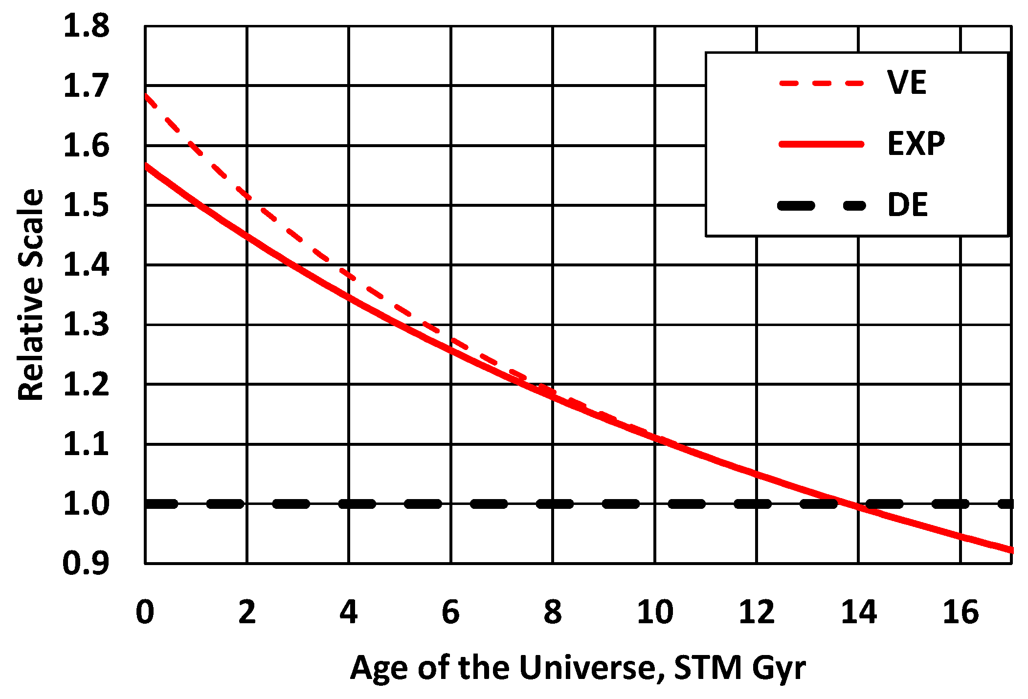

Table 1.
Cosmological parameter fits to the DESI data in the flat w0waCDM model, from Son et al [7]. The fits are arranged so the top rows use the least amount of scale-dependent data, and the bottom rows have the most scale-dependence. An SN age correction of -0.030 ± 0.004 mag/Gyr was used for the right two columns. The uncorrected data for the fits to w0 and wa show a clear trend of change with scale-dependence, most clearly the w0 values becoming more negative with increasing scale dependence. The age-corrected fits are consistent with each other, within the fit parameter uncertainty. These results are plotted in Figure 2 for visual comparison.
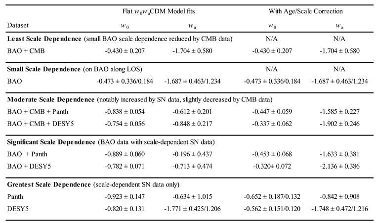 |
Disclaimer/Publisher’s Note: The statements, opinions and data contained in all publications are solely those of the individual author(s) and contributor(s) and not of MDPI and/or the editor(s). MDPI and/or the editor(s) disclaim responsibility for any injury to people or property resulting from any ideas, methods, instructions or products referred to in the content. |
© 2026 by the authors. Licensee MDPI, Basel, Switzerland. This article is an open access article distributed under the terms and conditions of the Creative Commons Attribution (CC BY) license (http://creativecommons.org/licenses/by/4.0/).
Copyright: This open access article is published under a Creative Commons CC BY 4.0 license, which permit the free download, distribution, and reuse, provided that the author and preprint are cited in any reuse.


