Causal Set Approach to AQFT

1. Introduction: AQFTs

Many QFTs, including non-linear $\mathsf{\Sigma }$-models, topological quantum field theories (TQFTs), and algebraic quantum field theories (AQFTs) are essentially functorial; i.e., the theories can be realized as a functor:

$$\mathcal{Z}:\mathcal{S}⟶\mathcal{T}$$

(1.1)

between (typically symmetric monoidal) categories. For instance, if we take $\mathcal{S}$ to be the category ${\mathbf{Loc}}_m$ of $m=(n+1)$-dimensional spacetimes and $\mathcal{T}$ to be the category ${}^{*}\mathbf{Alg}_{\mathbb{C}}$ of complex *-algebras, then we recover the Benini–Perin–Schenkel (BPS) formalism (a type of axiomatic AQFT) from [2]. However, the BPS model is actually a special case of Fewster–Verch [9,10], in which $\mathcal{Z}$ becomes a functor:

$$\mathcal{A}:\mathbf{Loc}⟶\mathsf{Phys}$$

(1.2)

where $\mathsf{Phys}$ is a “suitable category of physical systems," i.e., $\mathbf{Alg}$ or ${\mathbf{C}}^{*}-\mathbf{Alg}$. The specific algebra will always be a subalgebra of the algebra of all bounded operators on a Hilbert space, which is denoted in the literature by $B\left(\mathcal{H}\right)$.

Definition 1.1. 

The category $\mathbf{Loc}$ has:

1. 

Objects: quadruples $\mathbf{M}=(\mathcal{M},\mathbf{g},\mathfrak{o},\mathfrak{t})$ where: $(\mathcal{M},\mathbf{g})$ is a nonempty (smooth paracompact globally hyperbolic Lorentzian) spacetime of spacetime dimension m with at most finitely many connected components $\mathfrak{o}$ is a choice of orientation $\mathfrak{t}$ is a choice of time-orientation

2. 

Morphisms: smooth isometric embeddings, preserving both orientations, with causally convex image

Rather than being implemented “by hand," the observables of the theory are given in terms of elements $\gamma$ of algebras assigned by sub-theories ${\mathcal{B}}_i\subset \mathcal{A}$ which obey a few key axioms, including the Reeh-Schlieder theorem [6,9,10,15] of the vacuum representation, and Einstein causality [2,15]. The key property of $\gamma$ means it satisfies the identity:

$$\left|\right|{\gamma }^{*}\gamma \left|\right|={\left|\right|\gamma \left|\right|}^2$$

(1.3)

which is known as the $C^{*}$-property. Further, AQFTs are generally expected to satisfy another property, known as isotony, which states that if $O_1\subset O_2$ is an inclusion of spacetime regions, then there is an inclusion of algebras given by $\mathcal{A}\left(O_1\right)\subset \mathcal{A}\left(O_2\right)$.1

A popular choice for local quantum physics (LQP) is to let each ${\mathcal{B}}_i\left(\mathbf{M}\right)\subset \mathcal{A}\left(\mathbf{M}\right)$ be chosen such that we have an inclusion ${\mathbf{M}}_i:\mathbf{M}$ where ${\mathbf{M}}_i$ are the sub-objects of $\mathbf{M}$ such that

$${\mathbf{M}}_i\equiv ({\mathcal{N}}_i\subset \mathcal{M},\mathbf{g},\mathfrak{o},\mathfrak{t}).$$

(1.4)

Then, $\mathcal{M}$ is the universal spacetime, and the ${\mathcal{N}}_i$ are then an orientation-preserving localizations of $\mathcal{M}$.

Usually, we would want to consider diffeomorphisms2 of spacetimes ${\mathcal{M}}_f\simeq {\mathcal{M}}_g$ granted by considering isomorphic theories

$${\mathcal{B}}_{i,f}\left(\mathsf{\ell }\right)\cong {\mathcal{B}}_{i,g}\left(\mathsf{\ell }\right)$$

(1.5)

and thus promote the (Cauchy) morphisms of $\mathbf{Loc}$ to isomorphisms in the algebra category. This latter property is known as the “timeslice axiom" [9,10].

Example 1.1. 

Let $\mathcal{M}$ be an Alexandrov double-cone (causal diamond) in Minkowski space; then, the ${\mathcal{N}}_i$ that preserve both orientations are the sublightcones including subsets of the past, future, and present strata of $\mathcal{M}$. Then, our nets assign algebras of observables to every ℓ-local point, where

$$\mathsf{\ell }={\mathcal{M}}^{+}\cap {\mathcal{M}}^{-}$$

(1.6)

is the present region.3

In other words, we have a minimal algebra of observables given by ${\mathcal{B}}_N\left(\mathsf{\ell }\right)$, and a nested chain of embeddings ${\mathcal{B}}_N\left(\mathsf{\ell }\right)\hookrightarrow {\mathcal{B}}_{N-1}\hookrightarrow ...\hookrightarrow {\mathcal{B}}_0$ where N is the number of connected components4 of ${\mathcal{N}}_0$, acting as a finite cutoff to ensure that the physics is coherent.

Let ${\mathcal{N}}_{i,1}$ and ${\mathcal{N}}_{i,2}$ be two causally disjoint components of the global lightcone; then, pick representatives $a\in {\mathcal{B}}_{i,1}\left(\mathsf{\ell }\right)$ and $b\in {\mathcal{B}}_{i,2}\left(\mathsf{\ell }\right)$; Einstein causality5 tells us that they commute:

$$[a,b]=0.$$

(1.7)

Finally, one assumes translation covariance and the spectrum condition in the vacuum sector. Concretely, let $U\left(a\right)=e^{i{a}^{\mu }{P}_{\mu }}$ be a strongly continuous unitary representation of spacetime translations on $\mathcal{H}$ implementing covariance. The spectrum condition is that the joint spectrum of the generators $P_{\mu }$ lies in the closed forward lightcone. The vacuum vector $\mathsf{\Omega }$ is invariant under translations,

$$U\left(a\right)\mathsf{\Omega }=\mathsf{\Omega }\mathrm{for}\mathrm{all}\mathrm{translations}a,$$

(1.8)

and is unique up to a phase.

2. Causal Sets

In a flat Minkowski spacetime, there is a ready-made description in terms of causal sets (causets). The macroscopic, manifoldlike structure of the spacetime arises as a faithfully embeddable limit of causets. In this language, spacetime points $x\in {\mathbb{M}}^4$ are called events. Then, a causal set is defined by

$$C=(\mathcal{E},\prec )$$

(2.1)

where $\mathcal{E}$ is a set of events (typically countable and locally finite); for intuition one may consider a labeled subset ${\left\{x_i\right\}}_{i\in \mathbb{Z}}\subseteq \mathcal{E}$, but no global labeling is assumed and ≺ is an order relationship satisfying6:

• (transitivity): $x\prec y\prec z\Rightarrow x\prec z$
• (local finiteness) for all $x,z\in \mathcal{E}$ with $x\prec z$, the Alexandrov interval

  $$I(x,z)\{y\in \mathcal{E}\mid x\prec y\prec z\}$$

  is finite.
• (irreflexivity) $\nexists x\in \mathcal{E}\mathrm{such}\mathrm{that}x\prec x$.

Definition 2.1. 

Given a causal set $C=(\mathcal{E},\prec )$, the Alexandrov topology ${\tau }_A$ is the topology generated by sets of the form

$$I(x,y)=\{z\in \mathcal{E}|x\prec z\prec y\}.$$

Remark 2.1. 

The topology is derived, not assumed; ergo, no manifold structure or Hausdorff property is required.

Definition 2.2. 

A space ${\mathbb{K}}^n$ equipped with k time dimensions is denoted by ${\mathbb{K}}^{n+k}$ and is called a spacetime.

Two points in a spacetime comparable by the order $x\prec y$ are said to be causally related, and are often additionally required (in sequential growth dynamics) to satisfy Bell causality.7. For two causally related spacetime points, x is said to be “in the past" of y (or called an ancestor of y), and y is said to be “in the future" (or a descendant of x) if $x\prec y$.

Example 2.1. 

One may model a discrete “time axis” by a chain ${\left\{x_i\right\}}_{i\in \mathbb{Z}}$ with $x_i\prec x_j\iff i<j$. This is only a simplifying example and is not assumed in the general causal set framework.

2.1. Past-Step Modalities and Factorial Damping

Notation 2.1. 

Write $y\prec ·x$ if $y\prec x$ and there is no z with $y\prec z\prec x$. We call $\prec ·$ the link relation. For $n\in \mathbb{N}$, let

$${\mathrm{Past}}_n\left(x\right):=\{y\in \mathcal{E}:\exists x_0,\dots ,x_n\mathit{with}{x}_0=y,x_n=x,\mathrm{and}{x}_0\prec ·x_1\prec ·\dots \prec ·x_n\}.$$

(2.2)

We also set ${\mathrm{Past}}_0\left(x\right):=\left\{x\right\}$.

Definition 2.3. 

For each $n\in {\mathbb{N}}_0$ define an n-step past necessity modality $P_n$ by

$$x\vDash P_n\phi ⟺\forall y\in {\mathrm{Past}}_n\left(x\right),y\vDash \phi .$$

(2.3)

We emphasize that $P_n$ is indexed by n; it is not an inverse power of a single operator.8

Definition 2.4. 

Let $f:\mathcal{E}\to \mathbb{C}$ be a (field / observable-valued) function on events. Define the past-link adjacency operator B by

$$\left(Bf\right)\left(x\right):=\sum _{y\prec ·x}f\left(y\right).$$

(2.4)

Then $B^{n}f\left(x\right)$ is a sum over length-n link-chains ending at x (counting multiplicity of chains).

Axiom 2.1 

(Factorially damped past influence). Fix a coupling parameter $\lambda \in \mathbb{C}$. The total influence of past events on the present is encoded by the exponential generating operator

$$U\left(\lambda \right):=e^{\lambda B}=\sum _{n\ge 0}{\displaystyle \frac{{\lambda }^n}{n!}}{B}^n.$$

(2.5)

Thus the contribution from events n link-steps in the past is weighted by $1/n!$ (up to ${\lambda }^n$), and the overall past influence at x is $\left(U\right(\lambda \left)f\right)\left(x\right)$.

Remark 2.2. 

This gives a canonical discrete causal propagator on the Hasse diagram, compatible with link-composition and suitable for transporting local algebraic data along the net.

Remark 2.3. 

The factorial weighting is not imposed ad hoc: it is exactly what makes U compose cleanly as a one-parameter semigroup,

$$U\left(\lambda \right)U\left(\mu \right)=U(\lambda +\mu ),$$

(2.6)

which is the discrete-causal analogue of propagating influence through “elapsed causal depth.” By contrast, treating the individual coefficients ${\displaystyle \frac{1}{n!}}{B}^n$ as literal “powers” does not respect composition without extra binomial factors.

Main result: finite propagation, covariance, and truncation

The operator $U\left(\lambda \right)=e^{\lambda B}$ is the technical hinge connecting modal damping to AQFT-style local propagation. On a finite causet region it is automatically well-defined (as a finite polynomial in B), and its action admits an explicit causal kernel.

Theorem 2.1 

(Causal support and covariance of the factorial propagator). Let $C=(\mathcal{E},\prec )$ be a causal set and let $I\subseteq \mathcal{E}$ be a finite Alexandrov interval (or, more generally, any finite causally convex subset). Let B be the past-link adjacency operator restricted to I, and define $U\left(\lambda \right)=e^{\lambda B}$ as in (2.5). Then:

1. 

(Finite propagation / causal support). For every $x\in I$ and every function $f:I\to \mathbb{C}$,

$$\left(U\left(\lambda \right)f\right)\left(x\right)=\sum _{y\in I,y⪯x}{K}_{\lambda }(x,y)f\left(y\right),$$

(2.7)

where

$$K_{\lambda }(x,y):=\sum _{n\ge 0}{\displaystyle \frac{{\lambda }^n}{n!}}{N}_n(y⇝x),$$

(2.8)

and $N_n(y⇝x)$ is the number of link-chains of length n from y to x. In particular, $K_{\lambda }(x,y)=0$ unless y lies in the causal past of x.

2. 

(Polynomiality on finite regions). If $\left|I\right|=N$, then $B^N=0$ on I (equivalently, B is nilpotent), hence

$$U\left(\lambda \right)=\sum _{n=0}^{N-1}{\displaystyle \frac{{\lambda }^n}{n!}}{B}^n$$

(2.9)

is a finite sum.

3. 

(Discrete covariance). If $g:I\to I$ is an order-automorphism (a poset automorphism), and $(g·f)\left(x\right):=f\left(g^{-1}x\right)$ is the induced action on functions, then

$$U\left(\lambda \right)(g·f)=g·\left(U\right(\lambda \left)f\right).$$

(2.10)

Proof. (1) Expanding (2.5) gives $U\left(\lambda \right)f={\sum }_{n\ge 0}{\displaystyle \frac{{\lambda }^n}{n!}}{B}^{n}f$. By definition of B, the value $\left(B^{n}f\right)\left(x\right)$ is a sum of $f\left(y\right)$ over length-n link-chains $y=x_0\prec ·x_1\prec ·\dots \prec ·x_n=x$; collecting coefficients yields (2.7)–(2.8), and shows $y⪯x$ is necessary. (2) Choose any linear extension of ⪯ on I; then B is strictly lower triangular in that basis, hence nilpotent with index at most N, giving (2.9). (3) An order-automorphism preserves link relations, so it conjugates B (and hence $B^n$) under the pullback action on functions. Therefore $U\left(\lambda \right)=\sum {\displaystyle \frac{{\lambda }^n}{n!}}{B}^n$ commutes with the action, giving (2.10). □

Corollary 2.1 

(Locality of influence). For $x\in I$, the value $\left(U\right(\lambda \left)f\right)\left(x\right)$ depends only on the restriction of f to the causal past $\{y\in I:y⪯x\}$.

Corollary 2.2 

(A simple truncation bound). Equip functions $f:I\to \mathbb{C}$ with the sup norm ${\parallel f\parallel }_{\infty }={sup}_{x\in I}\left|f\left(x\right)\right|$, and let $\Delta :={max}_{x\in I}\#\{y\in I:y\prec ·x\}$ be the maximal past-link degree. Then ${\parallel Bf\parallel }_{\infty }\le \Delta {\parallel f\parallel }_{\infty }$. Consequently, for any $k\ge 0$ the truncated propagator $U_{\le k}\left(\lambda \right):={\sum }_{n=0}^k{\displaystyle \frac{{\lambda }^n}{n!}}{B}^n$ satisfies

$$\parallel (U\left(\lambda \right)-U_{\le k}\left(\lambda \right)){f\parallel }_{\infty }\le \left(\sum _{n=k+1}^{N-1}{\displaystyle \frac{{\left|\lambda \right|}^n{\Delta }^n}{n!}}\right){\parallel f\parallel }_{\infty }.$$

(2.11)

Let $x\in {\mathbb{M}}^4$ be a point of Minkowski spacetime corresponding (under an embedding / sprinkling9) to an event $x_0\in \mathcal{E}$.

Definition 2.5. 

The present representative $x_0$ is a maximal element of a finite Alexandrov interval up to isomorphism.

Formally: fix a causet $C=(\mathcal{E},\prec )$ and a finite interval $I(x^{-},x^{+})$. The present representative is defined to be the $x_0\in I(x^{-},x^{+})$ which is maximal w.r.t. ≺. Any two such choices are declared equivalent if they are related by an automorphism of the induced subposet.

Remark 2.4. 

The above gives us gauge freedom, and is meaningful from a LQP perspective. No global present is assumed or required.

We interpret $x_0$ as a present representative for the fixed interval $I(x^{-},x^{+})$, i.e. a gauge-chosen “necessary” frame organizing modal accessibility within that interval, reminiscent of [5].

Denote the set of present (necessary) events by $C_{/\square }\subseteq \mathcal{E}$, and write $x_0\in C_{/\square }$. To relate this to the causal order, fix a choice of a past-directed link-chain

$$x_{-n}\prec ·x_{-(n-1)}\prec ·\dots \prec ·x_{-1}\prec ·x_0,n\in \mathbb{N},$$

so that $x_{-n}\in {\mathrm{Past}}_n\left(x_0\right)$ in the sense of Notation 2.1.10

We also consider two auxiliary collections of events:

• $C_{/♢}^{-}\subseteq \mathcal{E}$, the previously possible events11;
• $C_{/♢}^{+}\subseteq \mathcal{E}$, the future-possible events.

Their intersection

$$C_{/♢}^0:=C_{/♢}^{-}\cap C_{/♢}^{+}$$

is interpreted as the “kinematically admissible” present slice (possible from both past and future perspectives). We assume that the necessary present sits inside this admissible slice:

$$C_{/\square }\subseteq C_{/♢}^0.$$

Axiom 2.2. 

(Reflexive necessity) The present event is 0-steps from itself, i.e. ${\mathrm{Past}}_0\left(x_0\right)=\left\{x_0\right\}$. Past dependence is encoded by the indexed past modalities $P_n$ (Definition 2.3), rather than by negative powers of □. Concretely, $P_n\phi$ expresses a necessity condition12 on all events n link-steps in the past of $x_0$.

Remark 2.5. 

Heuristically, a chosen past chain ${\left(x_{-n}\right)}_{n\in \mathbb{N}}$ may be viewed as a directed approximation of the present event $x_0$ from the past.

2.2. Locally Covariant Nets on Causal Sets

The abstract causal–modal framework developed above admits a direct reformulation in the language of algebraic quantum field theory once spacetime regions are replaced by suitable order-theoretic domains. In this subsection we construct a net of local algebras over a causal set and formulate discrete analogues of the Haag–Kastler axioms, thereby reconnecting the modal lightcone formalism with AQFT proper.

2.2.1. Nets on Causal Sets

Let $(\mathcal{C},⪯)$ be a locally finite causal set. Let $\mathbf{Int}\left(\mathcal{C}\right)$ denote the category whose objects are finite Alexandrov intervals $I(x,y)\subset \mathcal{C}$ and whose morphisms are inclusions $I(x,y)\hookrightarrow I(x^{\prime },y^{\prime }).$ We use the Alexandrov topology ${\tau }_A$ of Definition 2.1 only as a derived notion of locality.

A net of local algebras on $\mathcal{C}$ is a covariant functor

$$\mathcal{A}:\mathbf{Int}\left(\mathcal{C}\right)⟶\mathsf{Phys},$$

(2.12)

where $\mathsf{Phys}$ denotes a category of physical systems, such as unital *-algebras or $C^{*}$-algebras. To each Alexandrov interval $I(x,y)$ the functor assigns a local algebra

$$I(x,y)⟼\mathcal{A}\left(I\right(x,y\left)\right),$$

(2.13)

interpreted as the algebra of observables localized within the causal diamond determined by x and y.

Functoriality is implemented via inclusions of intervals:

$$I(x,y)\subseteq I(x^{\prime },y^{\prime })\Rightarrow \mathcal{A}\left(I(x,y)\right)\hookrightarrow \mathcal{A}\left(I(x^{\prime },y^{\prime })\right).$$

(2.14)

These inclusions are induced by order-theoretic containment of Alexandrov intervals, ensuring that algebraic localization respects the discrete causal structure.

Remark 2.6 

(Why the causal set formulation is not merely a translation). Working over $\mathbf{Int}\left(\mathbf{C}\right)$ is not only a cosmetic replacement of open subsets of a manifold by order-theoretic regions. In a general causal set there is no canonical notion of Cauchy surface, nor a preferred differential structure, and even the availability of “time-slice” hypersurfaces becomes a genuinely nontrivial condition. Moreover, locality and causal disjointness become purely order-theoretic constraints, and the factorially damped modal operator $U\left(\lambda \right)=exp\left(\lambda B\right)$ supplies a canonical (and tunable) mechanism for controlled propagation along the Hasse diagram. In this sense the causal set axioms below encode genuinely discrete content rather than a formal rephrasing of the continuum Haag–Kastler setup.

2.2.2. Discrete Haag–Kastler Axioms

Within this framework, the Haag–Kastler axioms admit natural reformulations adapted to the partial order ⪯.

Isotony.

For any pair of intervals $I_1,I_2\subset \mathcal{C}$,

$$I_1\subseteq I_2\Rightarrow \mathcal{A}\left(I_1\right)\subseteq \mathcal{A}\left(I_2\right).$$

(2.15)

Einstein causality.

If two intervals $I_1=I(x_1,y_1)$ and $I_2=I(x_2,y_2)$ are spacelike separated in the sense that no event of $I_1$ is comparable to any event of $I_2$ (i.e. for all $a\in I_1$ and $b\in I_2$, neither $a⪯b$ nor $b⪯a$ holds), then the corresponding algebras commute:

$$[\mathcal{A}\left(I_1\right),\mathcal{A}\left(I_2\right)]=0.$$

Time-slice axiom (discrete).

Assume $\mathcal{C}$ admits a causally convex slice S intersecting every maximal chain in a chosen finite region exactly once.

Then,

$$\mathcal{A}\left(I\right)=\mathcal{A}\left(S\right),\mathrm{for}\mathrm{every}\mathrm{interval}I\supseteq S,$$

(2.16)

denotes the $C^{*}$-algebra generated by the indicated subalgebras.

Property 2.1 

(Functoriality of factorially damped modal transport on intervals). Let C be a causal set and let $A:\mathbf{Int}\left(\mathbf{C}\right)\to \mathbf{Alg}$ be a causal net on Alexandrov intervals, with isotony maps

$${\iota }_{IJ}:A\left(I\right)\hookrightarrow A\left(J\right)\mathrm{for}I\subseteq J$$

in $\mathbf{Int}\left(\mathbf{C}\right)$. Fix $\lambda \in {\mathbb{R}}_{\ge 0}$ and assume that for each interval $I\in \mathbf{Int}\left(\mathbf{C}\right)$ the algebra $A\left(I\right)$ carries a (linear) action of the link-adjacency operator $B_I$ induced by the Hasse diagram of I (e.g. by acting on coefficient functions in a chosen presentation of $A\left(I\right)$), and define the factorially damped operator

$$U_I\left(\lambda \right):=exp\left(\lambda B_I\right)=\sum _{n\ge 0}{\displaystyle \frac{{\lambda }^n}{n!}}{B}_I^n$$

on $A\left(I\right)$. Then for every inclusion $I\subseteq J$ in $\mathbf{Int}\left(\mathbf{C}\right)$ the diagram

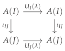commutes, i.e. ${\iota }_{IJ}\circ U_I\left(\lambda \right)=U_J\left(\lambda \right)\circ {\iota }_{IJ}$.

Proof. 

The inclusion $I\subseteq J$ induces an inclusion of Hasse diagrams (links inside I remain links when regarded inside J). Hence the adjacency operators are compatible in the sense that $B_J$ restricts to $B_I$ on the subinterval I, and therefore

$${\iota }_{IJ}\circ B_I=B_J\circ {\iota }_{IJ}.$$

By induction this implies ${\iota }_{IJ}\circ B_I^n=B_J^n\circ {\iota }_{IJ}$ for all $n\ge 0$. Applying this termwise to the exponential series gives

$${\iota }_{IJ}\circ U_I\left(\lambda \right)=\sum _{n\ge 0}{\displaystyle \frac{{\lambda }^n}{n!}}{\iota }_{IJ}\circ B_I^n=\sum _{n\ge 0}{\displaystyle \frac{{\lambda }^n}{n!}}{B}_J^n\circ {\iota }_{IJ}=U_J\left(\lambda \right)\circ {\iota }_{IJ},$$

as claimed. □

Corollary 2.3. 

The family ${\left\{U_I\left(\lambda \right)\right\}}_{I\in \mathbf{Int}\left(\mathbf{C}\right)}$ defines a natural endomorphism of the functor $A:\mathbf{Int}\left(\mathbf{C}\right)\to \mathbf{Alg}$. In particular, factorially damped modal transport is compatible with isotony, so that “evolving inside a smaller interval and then embedding” equals “embedding first and evolving inside the larger interval.”

Definition 2.6. 

For any causally convex subset $S\subseteq \mathcal{C}$, define

$$\mathcal{A}\left(S\right):=\underset{I\subseteq S}{\underrightarrow{lim}}\mathcal{A}\left(I\right),$$

the inductive limit over all finite Alexandrov intervals I contained in S.

Causal propagation along the net is implemented by the factorially damped operator of (2.5)

$$U\left(\lambda \right):=e^{\lambda B},$$

(2.17)

where B is the causal adjacency operator on the Hasse diagram of $\mathcal{C}$. This operator acts as a discrete causal propagator, implementing algebraic transport between successive layers of the net.

2.2.3. Cauchy Slices and the Necessary Present

The modal lightcone construction introduced earlier singles out distinguished slices of the causet. The necessary present slice $C_{/\square }$, together with the admissible slice $C_{/♢}^0$, play the role of discrete Cauchy surfaces. Each such slice determines a subalgebra

$$\mathcal{A}\left(C_{/\square }\right)\subseteq \mathcal{A}\left(\mathcal{C}\right),$$

(2.18)

from which the full net may be reconstructed via causal propagation.

This identification permits the formulation of initial-value problems, state selection, and vacuum-like conditions entirely within the causal-set framework. In this sense, the modal present functions as a discretized analogue of a global Cauchy hypersurface, anchoring the dynamical content of the theory.

Remark 2.7 

(Choice of local algebras). The abstract formulation above leaves open the precise nature of the objects of $\mathsf{Phys}$ and of the inclusions $\mathcal{A}\left(I_1\right)\hookrightarrow \mathcal{A}\left(I_2\right).$ From the perspective of algebraic quantum field theory, several natural choices present themselves.

• (i) $C^{*}$-algebras. A canonical choice is to take $\mathsf{Phys}$ to be the category of unital $C^{*}$-algebras with injective *-homomorphisms. In this case, $\mathcal{A}\left(I\right)$ is interpreted as the algebra of bounded observables measurable within the Alexandrov interval I, and isotony is realized as $C^{*}$-subalgebra inclusion. This choice aligns most closely with the Haag–Kastler framework and ensures the existence of well-behaved state spaces.
• (ii) von Neumann algebras. Alternatively, one may assign to each interval I a von Neumann algebra $\mathcal{A}\left(I\right)\subset \mathcal{B}\left(\mathcal{H}\right)$, obtained as the weak closure of a corresponding $C^{*}$-algebra in a chosen representation. In this setting, causal propagation along the net admits a natural modular-theoretic interpretation, and the discrete propagator $U\left(\lambda \right)$ may be compared with Tomita–Takesaki modular flows [4].
• (iii) Quasilocal algebra. The global algebra

  $$\mathcal{A}\left(\mathcal{C}\right):=\overline{\bigcup _{I\subset \mathcal{C}}\mathcal{A}\left(I\right)}$$

  (2.19)

  is naturally interpreted as the quasilocal algebra of the theory, where the closure is taken in the norm topology. Subalgebras associated with slices such as $C_{/\square }$ or $C_{\langle ♢\rangle }^0$ then serve as candidates for initial-data algebras, from which the full net may be reconstructed via causal propagation.
• (iv) Subalgebras and localization. For any causally convex subset $S\subset \mathcal{C}$, the associated algebra $\mathcal{A}\left(S\right)$ should be understood as the inductive limit of the algebras $\mathcal{A}\left(I\right)$ over all Alexandrov intervals $I\subset S$. This ensures that localization is stable under refinement of the causal domain and is compatible with the discrete time-slice axiom.
  In all cases, the causal set structure provides a canonical notion of locality, while the choice of algebraic category determines the analytical and representational content of the theory. The framework is therefore flexible enough to accommodate both kinematical constructions and dynamical state-selection schemes.

3. Dynamical and Other Aspects of Causets

Thus far, the above description has been purely kinematic; thus, it cannot be said to be a full theory of physics. We are impelled by classical wisdom now to describe the dynamics of the theory, in a way that is consistent with both the frameworks of causets and those of AQFT.

It has been suggested by Sorkin that time itself (also dubbed “growth" or cosmological accretion) is a stochastic process, akin to Brownian motion [14]. This view was taken up by Sorkin and Rideout in [12], and it involves fixing an unphysical “external time” (ET) parameter, which plays the rôle of a gauge variable. ET is constituted by a labelling of the events $x_i$ by a function ${\mathrm{label}}_i\left(x\right)$ satisfying

$$x_i\prec y_i\Rightarrow {\mathrm{label}}_i\left(x\right)\prec {\mathrm{label}}_i\left(y\right).$$

The analogue of gauge invariance (dubbed discrete general covariance) is then the slogan “labels are unphysical."

The authors of [12] concluded that the transition probability ${\alpha }_n$ from a causet ${\mathcal{C}}_n$ to any ${\mathcal{C}}_{n+1}$ is given by

$${\alpha }_n=p^m{(1-p)}^{n-\varpi }$$

(3.1)

whence there are m maximal elements in ${\mathcal{C}}_n$ and $\varpi$ is the size of the entire precursor set. Some care is then taken to ensure that the discrete general covariance holds, and that the Einstein-Bell causality is satisfied.

The authors themselves note that this description does not obviously translate into a notion of gauge invariance on a resulting manifold. One route there would be to consider each collection of chains (bounded region X) as a $T_0$-topological space with a poset-structure [11]. This effectively amounts to taking an enrichment ${\mathcal{C}}_{\mathbf{Top}}$ of the causet category from (2.12). The poset relation is then given by $x\to y$, which means “the convergence of the constant sequence $\left(x\right)$ to y in the $T_0$ topology of P", where P is the quotient of X by an equivalence relation between events.13 This enrichment supplies the minimal topological and categorical structure needed to pass from bare causal order to algebraic localization.

Given such a finitary $T_0$-poset P, a standard algebraic avatar of its causal-topological information is the (Rota) incidence algebra

$$\mathsf{\Omega }\left(P\right):={\mathrm{span}}_{\mathbb{C}}\{p\to q:p,q\in P\},$$

(3.2)

equipped with the associative product induced by concatenation of composable arrows:

$$(p\to q)·(r\to s):=\left\{\begin{array}{cc}p\to s\hfill & \mathrm{if}q=r,\hfill \\ 0\hfill & \mathrm{otherwise}.\hfill \end{array}\right.$$

(3.3)

The passage $P⇝\mathsf{\Omega }\left(P\right)$may be regarded as a quantization of the underlying finitary causal topology itself, since the causal arrow-relations $p\to q$ now admit coherent superpositions in the $\mathbb{C}$-linear envelope $\mathsf{\Omega }\left(P\right)$.

To recover a notion of “(quantum) points,” one passes to the primitive spectrum $\mathrm{Prim}\left(\mathsf{\Omega }\right(P\left)\right)$, identifying points with kernels of irreducible finite-dimensional representations of $\mathsf{\Omega }\left(P\right)$. A corresponding finitary topology is then induced on $\mathrm{Prim}\left(\mathsf{\Omega }\right(P\left)\right)$ by a relation generated intrinsically from the noncommutative product structure14 of $\mathsf{\Omega }\left(P\right)$. In this way, one spatializes the algebraic data back into a topological object, but now in a manner that is sensitive to the noncommutativity which encodes quantum interference of causal connections.

Moreover, $\mathsf{\Omega }\left(P\right)$ carries a natural ${\mathbb{Z}}_{\ge 0}$-grading

$$\mathsf{\Omega }\left(P\right)={\mathsf{\Omega }}^0\oplus {\mathsf{\Omega }}^1\oplus {\mathsf{\Omega }}^2\oplus \cdots ,$$

(3.4)

where ${\mathsf{\Omega }}^0$ may be viewed as a discrete algebra of “coordinates” on P, and ${\mathsf{\Omega }}^{\ge 1}$ as higher-degree discrete differential forms. In this framework, bounded causet regions X may be endowed not only with finitary causal-topological structure, but also with a discrete differential calculus, providing a principled route from purely order-theoretic kinematics to geometric field content.

At this stage, one may combine the kinematical locality of AQFT with the stochastic “growth” dynamics of causal sets as follows. To each bounded region X (e.g. a suitable collection of chains, or a causally convex subcauset), we associate a finitary $T_0$-poset $P_X$, and hence an incidence algebra $\mathsf{\Omega }\left(P_X\right)$. Thus one obtains an algebra assignment

$$X⟼\mathsf{\Omega }\left(P_X\right),$$

(3.5)

which is contravariantly compatible with refinement of regions (or, dually, covariantly compatible with coarse-graining). This has precisely the net-like shape expected in AQFT: smaller regions determine subalgebras or restriction maps, and global information is assembled from local data.

Finally, the Rideout–Sorkin sequential growth dynamics supplies a natural probabilistic law on the space of finite causet histories. Note that each growth step ${\mathcal{C}}_n\to {\mathcal{C}}_{n+1}$ induces, after passage through the finitary $T_0$-poset representation, a corresponding transition of local algebraic data associated to bounded regions.

$$\mathsf{\Omega }\left(P_n\right)⟶\mathsf{\Omega }\left(P_{n+1}\right),$$

(3.6)

and hence a stochastic evolution not merely of events, but of the algebraic carriers of causal information themselves. In this way, one may regard the growth law as generating a dynamical measure on nets of local incidence algebras, giving a concrete sense in which “labels are unphysical” becomes compatible with a gauge-like covariance principle at the algebraic level.

4. Future Work

The present manuscript has focused on a concrete kinematical package: (i) a factorially damped causal propagator $U\left(\lambda \right)=e^{\lambda B}$ with finite propagation and discrete covariance (Proposition 2.1), and (ii) a causet-indexed net of local algebras satisfying discrete Haag–Kastler-type axioms. What remains is to (a) strengthen these structures into a representation-theoretic AQFT, and (b) connect them to genuine dynamics. We record three focused directions.

4.1. Deepening the Modal Structure of Causet Nets

The modal lightcone formalism can be made less semantic and more structural by treating the indexing category itself as carrying modal data. Concretely, one can:

• define a modal enrichment of $\mathbf{Int}\left(\mathcal{C}\right)$ (e.g. by adding accessibility morphisms between intervals determined by admissible slices);
• impose compatibility conditions between the modal operators $P_n$ and the algebra maps $\mathcal{A}\left(I_1\right)\hookrightarrow \mathcal{A}\left(I_2\right)$ (so that modal restriction/extension is functorial);
• study whether the propagator $U\left(\lambda \right)$ intertwines modal refinement, i.e. whether it acts naturally on modalized subalgebras associated to slices such as $C_{/\square }$.

The goal is to replace informal “necessity/possibility” language by explicit functorial data that can be checked on finite regions.

4.2. Dynamics via Sheaf-Localization and Gauge Data

The sequential growth law supplies a measure on causet histories, but does not immediately specify how local algebras evolve. A concrete next step is to evolve pairs $({\mathcal{C}}_n,{\mathcal{A}}_n)$ rather than bare causets ${\mathcal{C}}_n$. One route is:

• represent bounded regions by finitary $T_0$-posets $P_X$ and assign incidence algebras $\mathsf{\Omega }\left(P_X\right)$;
• organize these assignments as a sheaf (or stack) over refinements of regions, so that restriction maps become part of the data;
• introduce discrete connection-like transport between overlaps, and compare it against the intrinsic transport encoded by $U\left(\lambda \right)$.

This reframes “dynamics” as a local-to-global compatibility problem for algebraic carriers, in which curvature-type obstructions can be defined purely finitarily.

4.3. Continuum Limits, Reconstruction, and Comparison to Haag–Kastler Axioms

To compare with continuum AQFT, one needs explicit reconstruction criteria rather than informal “sprinkling limits.” Useful near-term targets include:

• a discrete additivity condition (generation of $\mathcal{A}\left(I\right)$ from subinterval algebras) and its stability under refinement;
• an explicit covariance statement for embeddings of finite intervals (compatible with Proposition 2.1(3));
• representation-theoretic input: existence of physically meaningful states and a causet analogue of the spectrum condition.

These are the points at which one can begin proving that the discrete net converges (in an appropriate sense) to a Haag–Kastler net in a continuum approximation.

Appendix A.1. The Diamond Poset and Its Adjacency Operator

Consider the four-element “diamond” causet with events $\{a,b,c,d\}$ and order relations

$$a\prec b,a\prec c,b\prec d,c\prec d,$$

(A1)

with no other comparabilities. Equivalently, the Hasse diagram consists of the four link relations $a\prec ·b$, $a\prec ·c$, $b\prec ·d$, $c\prec ·d$.

Let $f:\{a,b,c,d\}\to \mathbb{C}$ be any function. By Definition 2.4, the past-link adjacency operator B acts as

$$\begin{array}{cc}\hfill \left(Bf\right)\left(a\right)& =0,\hfill \end{array}$$

(A2)

$$\begin{array}{cc}\hfill \left(Bf\right)\left(b\right)& =f\left(a\right),\hfill \end{array}$$

(A3)

$$\begin{array}{cc}\hfill \left(Bf\right)\left(c\right)& =f\left(a\right),\hfill \end{array}$$

(A4)

$$\begin{array}{cc}\hfill \left(Bf\right)\left(d\right)& =f\left(b\right)+f\left(c\right).\hfill \end{array}$$

(A5)

Applying B twice yields

$$\begin{array}{cc}\hfill \left(B^{2}f\right)\left(a\right)& =0,\hfill \end{array}$$

(A6)

$$\begin{array}{cc}\hfill \left(B^{2}f\right)\left(b\right)& =0,\hfill \end{array}$$

(A7)

$$\begin{array}{cc}\hfill \left(B^{2}f\right)\left(c\right)& =0,\hfill \end{array}$$

(A8)

$$\begin{array}{cc}\hfill \left(B^{2}f\right)\left(d\right)& =2f\left(a\right),\hfill \end{array}$$

(A9)

since there are precisely two distinct length-2 link-chains from a to d (namely $a\to b\to d$ and $a\to c\to d$). One checks immediately that $B^3=0$ on this causet.

Appendix A.2. The Factorial Propagator

Because $B^3=0$, the exponential truncates exactly:

$$U\left(\lambda \right)=e^{\lambda B}=⊮+\lambda B+{\displaystyle \frac{{\lambda }^2}{2}}{B}^2.$$

(A10)

Therefore

$$\begin{array}{cc}\hfill \left(U\right(\lambda \left)f\right)\left(a\right)& =f\left(a\right),\hfill \end{array}$$

(A11)

$$\begin{array}{cc}\hfill \left(U\right(\lambda \left)f\right)\left(b\right)& =f\left(b\right)+\lambda f\left(a\right),\hfill \end{array}$$

(A12)

$$\begin{array}{cc}\hfill \left(U\right(\lambda \left)f\right)\left(c\right)& =f\left(c\right)+\lambda f\left(a\right),\hfill \end{array}$$

(A13)

$$\begin{array}{cc}\hfill \left(U\right(\lambda \left)f\right)\left(d\right)& =f\left(d\right)+\lambda \left(f\left(b\right)+f\left(c\right)\right)+{\lambda }^{2}f\left(a\right).\hfill \end{array}$$

(A14)

The last line displays the causal-kernel interpretation from Proposition 2.1 explicitly: the coefficient of $f\left(a\right)$ at d is ${\lambda }^2$, coming from two length-2 chains weighted by ${\lambda }^2/2!$.

References

- Bombelli, L.; Lee, J.; Meyer, D.; Sorkin, R. D. Space-Time as a Causal Set. Physical Review Letters 1987, 59, 5. [Google Scholar] [CrossRef] [PubMed]
- Benini, M.; Perin, M.; Schenkel, A. Smooth 1-dimensional algebraic quantum field theories. arXiv 2020, arXiv:2010.13808v2. [Google Scholar] [CrossRef]
- Benini, M.; Grant-Stuart, A.; Schenkel, A. Haag-Kastler stacks Communications in Contemporary Mathematics (2025) 2550099. [CrossRef]
- Borchers, H. J. On Revolutionizing of Quantum Field Theory with Tomita’s Modular Theory Vienna, Preprint ESI 773 (1999). Available online: https://www.esi.ac.at/preprints/esi773.pdf.
- Buchanan, R. J. (p,q)-String Junctions as Interstitial Fields on a Modal Lightcone. [CrossRef]
- Doplicher, S.; Haag, R.; Roberts, J..E. Fields, Observables, and Gauge Transformations. Commun. math. Phys. 1969, 13, 1–23. [Google Scholar] [CrossRef]
- Dowker, F. Causal sets and the deep structure of spacetime. arXiv 2005. [Google Scholar] [CrossRef]
- Dowker, F.; Henson, J.; Sorkin, R. D. Quantum Gravity Phenomenology, Lorentz Invariance and Discreteness. Mod. Phys.Lett 2004, A19, 1829–1840. [Google Scholar]
- Fewster, C..J. Endomorphisms and automorphisms of locally covariant quantum field theories. Rev. Math. Phys. 2013, arXiv:1201.3295v225, 1350008. [Google Scholar] [CrossRef]
- Fewster, C. J.; Verch, R. Dynamical locality and covariance: What makes a physical theory the same in all spacetimes? Annales Henri Poincaré 2012, arXiv:1106.4785v313, 1613–1674. [Google Scholar] [CrossRef]
- Raptis, I. Quantum Space-Time as a Quantum Causal Set. arXiv 2002. [Google Scholar] [CrossRef]
- Rideout, D. P.; Sorkin, R. D. A Classical Sequential Growth Dynamics for Causal Sets. Phys.Rev. 2000, D61, 024002. [Google Scholar] [CrossRef]
- Sion, C.-L. The Haag-Kastler axiomatic framework. 2012. Available online: https://www.physik.uni-hamburg.de/th2/ag-fredenhagen/dokumente/thehaag-kastleraxiomaticframework.pdf (accessed on 24 June 2012).
- Sorkin, R. D. Causal Sets: Discrete Gravity (1 Sep, 2003) Report Number: SU-GP-2003/1-2 arXiv:gr-qc/0309009.
- Schroer, B. Lectures on Algebraic Quantum Field Theory and Operator Algebras. Notas de Física, Centro Brasileiro de Pesquisas Físicas, Rio de Janeiro, April 2001.
- Zapatrin, R. R. Incidence algebras of simplicial complexes. Pure Mathematics and Applications 2001, 11, 105–118. [Google Scholar]