
Submitted:
20 January 2026
Posted:
20 January 2026
You are already at the latest version
Abstract
We present a comprehensive spectral and kinematic analysis of 27 polluted white dwarfs selected from the catalog of polluted white dwarf candidates by \citep{2024MNRAS.527.4515B}. Using LAMOST DR9 and Gaia DR3 data, we derive the effective temperature ($T_{\mathrm{eff}}$), surface gravity ($\log g$), and radial velocity ($RV$), and measure the Ca\,\textsc{II}\,K line parameters, including equivalent width ($EW_{\mathrm{Ca\,II\,K}}$) and radial velocity ($RV_{\mathrm{Ca\,II\,K}}$). In addition, we estimate cooling ages and determine the three-dimensional Galactic kinematics and orbital parameters. Our results show that the majority of the targets lie above the pure-ISM expectation for the Ca\,\textsc{II}\,K line, suggesting that the line primarily originates from circumstellar material (CSM) rather than the interstellar medium (ISM). For DA-type white dwarfs in our sample, the Ca\,\textsc{II}\,K absorption is more prominent at lower effective temperatures and becomes significantly weaker toward higher temperatures, consistent with previous studies of metal-polluted white dwarfs. Additionally, DA stars show prominent $EW_{\mathrm{Ca\,II\,K}}$ values primarily in the cooling-age bin of $0.9$--$1.4\,\mathrm{Gyr}$, whereas DB stars are concentrated in the $\tau_{\mathrm{cool}} \lesssim 0.5\,\mathrm{Gyr}$ range, with a similar trend of first increasing and then decreasing $EW_{\mathrm{Ca\,II\,K}}$ with cooling age. Kinematic analysis reveals no significant differences between the Galactic populations of DA and DB white dwarfs. These findings indicate that metal pollution is common across different disk components of the Galaxy, with evidence for ongoing or recurrent evolution of white dwarf planetary systems within various Galactic structures.
Keywords:
white dwarfs
; polluted white dwarfs
; circumstellar material
; Ca II K absorption
; stellar kinematics
1. Introduction
White dwarfs are the final evolutionary products of low- and intermediate-mass stars (with initial masses –; [2]), representing the ultimate fate of about of all stars in the Milky Way [4]. A typical white dwarf has a mass of and a size comparable to that of Earth. Its extremely strong surface gravity leads to pronounced atmospheric stratification: elements heavier than helium rapidly sink out of the optically visible layers on timescales of – years, leaving atmospheres dominated by hydrogen or helium [3]. Nevertheless, observations reveal that about 25– of white dwarfs display photospheric heavy elements [5,6,7], a phenomenon referred to as metal pollution.
Given the short diffusion timescales of metals [8,9], these elements cannot be intrinsic remnants but must instead result from recent or ongoing external accretion. Our understanding of the origin of this pollution has undergone a paradigm shift—from early hypotheses invoking stellar winds or interstellar accretion to the now widely accepted model of accretion from planetary debris. Early studies proposed mechanisms such as wind accretion from a binary companion [10] or accretion during passage through interstellar clouds [11]. With growing sample sizes and multi-wavelength evidence, the consensus now favors the accretion of rocky planetary remnants: planets or minor bodies that survive the post-main-sequence evolution are dynamically scattered onto highly eccentric orbits, tidally disrupted, and subsequently form debris disks that feed heavy elements onto the white dwarf photosphere [see the review by [12]. This scenario is supported by multiple lines of observational evidence, including infrared excesses indicating dusty disks [13,14], double-peaked metal emission lines revealing gaseous disks [15], X-ray signatures of ongoing accretion [16], and direct JWST imaging of planetary companions around two polluted white dwarfs [17].
Polluted white dwarfs therefore provide a unique window into the late-stage evolution of planetary systems and the physics of accretion processes [18]. Large-scale surveys such as LAMOST and Gaia have greatly expanded the available samples. Against this backdrop, Badenas-Agusti et al. [1] cross-matched Gaia EDR3 with LAMOST DR9 to construct a catalog of 62 polluted white dwarfs. While that work provided preliminary characterizations, key questions remain unresolved—particularly regarding the origin of the Ca II K line, its distribution with the cooling ages, and the kinematic properties of these systems, all of which hold critical clues for understanding the nature and evolution of polluted white dwarfs. Motivated by this, we conduct a detailed analysis of the Ca II K line characteristics, cooling ages, and kinematics for a high-quality subsample of these objects.
2. Data and Sample Selection
2.1. Data
The data used in this study are drawn from two major astronomical surveys: LAMOST and Gaia. LAMOST (the Large Sky Area Multi-Object Fiber Spectroscopic Telescope; also known as the Guo Shoujing Telescope) is located at Xinglong Observatory, Hebei Province, China. It is a wide-field, multi-fiber spectroscopic facility capable of obtaining spectra simultaneously over a field of view of about 20 square degrees. The spectra cover the wavelength range of 3690– and are available in both low- and medium-resolution modes ( and ) [19]. To date, LAMOST has accumulated more than ten million stellar spectra [20], providing a crucial foundation for studies of Galactic stellar populations and peculiar objects.
Gaia, launched by the European Space Agency (ESA) in 2013, is a space-based astrometric mission that provides precise positions, parallaxes, proper motions, radial velocities, and multi-band photometry for over one billion stars across the Milky Way [21,22]. In this work, we use the astrometric and photometric data from its third major data release (Gaia DR3), which offers improved parallax precision, full five-parameter astrometry, extended radial velocity measurements, and detailed astrophysical parameters. Combined with the LAMOST radial velocities, these data allow us to derive accurate spatial positions and three-dimensional kinematics for the target white dwarfs.
Our initial sample is based on the catalog of polluted white dwarf candidates constructed by Badenas-Agusti et al. [1] through cross-matching LAMOST DR9 low-resolution spectra with Gaia EDR3 astrometric data. That study identified 62 candidates and provided preliminary spectral classifications and atmospheric parameters. Most of these objects have LAMOST spectra with high signal-to-noise ratios (S/N ), making them suitable for uniform and detailed spectral analysis.
2.2. Sample Selection
To ensure the reliability and consistency of our analysis, we performed a secondary screening of the 62 polluted white dwarf candidates identified by Badenas-Agusti et al. [1]. This selection relied primarily on visual inspection of the LAMOST low-resolution (LRS) spectra, focusing on both the spectral-type classification and the quality of the metallic absorption features. The screening procedure was conducted as follows:
- 1.
- Spectral screening. Each spectrum was visually inspected to assess the continuum shape and the presence of diagnostic absorption lines. Only spectra showing clear hydrogen (Balmer) or helium features were retained, because our spectral fitting used the DA and DB atmospheric model grids of Koester [23]. White dwarfs of the DZ type—dominated by metal lines and incompatible with the adopted grids—were excluded (29 objects). In addition, six misclassified sources whose spectral morphologies were inconsistent with those of typical white dwarfs were rejected.
- 2.
- Assessment of metal-line quality. During the same inspection, particular attention was given to the Ca II K line at and other metallic absorption features. Only spectra with sufficiently high signal-to-noise ratios () and well-defined line profiles were retained, ensuring reliable determinations of radial velocity and equivalent width () in the subsequent analysis.
After applying these criteria, a total of 27 polluted white dwarfs—comprising 17 DA and 10 DB types—fulfilled all selection requirements and were retained as the final working sample for detailed study.Their observational information and derived physical parameters are summarized in Table A1 and Table A2 in the Appendix.
3. Sample Analysis
This section presents the analysis of the final sample of 27 polluted white dwarfs. We describe the determination of their atmospheric parameters: effective temperature (), surface gravity (), and photospheric radial velocity (), as well as the measurement of the Ca II K () line parameters, including its radial velocity () and equivalent width (). We also infer the cooling ages () of these white dwarfs and compute their Galactic three-dimensional space velocities and orbital parameters to investigate their kinematic properties within the Milky Way.
3.1. Atmospheric Parameter and Radial Velocity Determination
We first degraded the theoretical DA and DB model spectra of Koester [23] to match the spectral resolution of the LAMOST observations. An initial estimate of the stellar radial velocity was obtained by performing a cross-correlation (CCF) between the resolution-matched model spectra and the observed LAMOST spectra. Using this preliminary radial velocity as the starting point, we then conducted a global spectral fitting to the LAMOST data to simultaneously derive the atmospheric parameters: effective temperature (), surface gravity () and the final radial velocity ().
However, it is well established that the spectroscopic technique based on 1D model atmospheres suffers from systematic biases due to the simplified treatment of convective energy transport, and that three-dimensional (3D) corrections are required for both DA and DB white dwarfs in specific effective temperature and surface gravity regimes.
For DA white dwarfs, we therefore applied the 1D-to-3D corrections presented by Tremblay et al. [24], which are based on CO5BOLD radiation–hydrodynamics simulations and are valid in the temperature range of approximately 6000–. These corrections were applied a posteriori to the spectroscopically derived and values.
For DB and DBA white dwarfs, we adopted the 3D correction functions provided by Cukanovaite et al. [25], which account for the effects of convection in helium-dominated atmospheres with trace hydrogen abundances. The corrections were computed using the publicly available Python implementation accompanying their work and were applied within the parameter ranges specified in that study.
After applying the appropriate 3D corrections, the atmospheric parameters reported in this work correspond to 3D-corrected values, thereby significantly reducing systematic offsets associated with the use of 1D model atmospheres.The measured atmospheric parameters and radial velocities for the 27 targets are presented in Appendix Table A1, while the spectral fitting plots can be found in Appendix B.
3.2. Measurement of Ca Line Velocity and Equivalent Width
Calcium is one of the most common and easily detectable metals in the atmospheres of polluted white dwarfs, making it an effective tracer for identifying and quantifying atmospheric metal pollution [26]. In particular, the LAMOST low-resolution spectra (LRS) cover multiple Ca transitions, including the doublet, the near-infrared triplet, and several weaker quadrupole lines.
However, due to the moderate spectral resolution () and the blending of these lines with nearby Balmer features such as H and the Paschen series, extracting and reliably analyzing the full set of Ca transitions is challenging. Among these, only the Ca line can be consistently separated from the blending features and analyzed with confidence [27]. Therefore, our analysis focuses exclusively on the Ca characteristics.
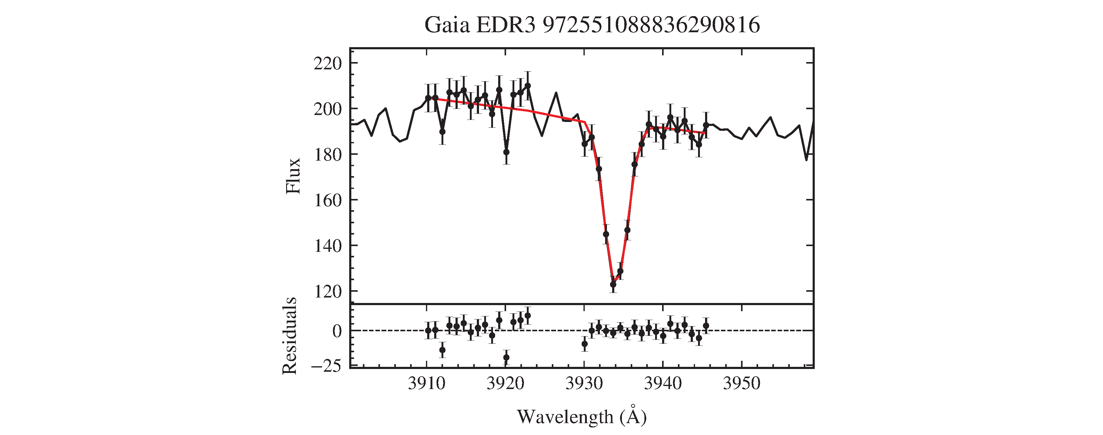
Following the method outlined in Li et al. [27], we measured the radial velocity () and equivalent width () of the Ca II K line. The line was modeled using a single Gaussian profile centered around the Ca II K line at , with a first-order polynomial included to represent the local continuum. The model is expressed as:
where A, , and represent the depth, centroid, and width of the Gaussian curve, respectively. The terms k and b describe the linear continuum of the observational spectrum.
The centroid shift of the Ca line relative to the rest wavelength provides the radial velocity (), while the equivalent width is derived from the integrated Gaussian area, normalized by the continuum level. To ensure robust uncertainty estimates for , we propagated the fitting errors using covariance matrix sampling. Specifically, random realizations of the best-fit parameters were drawn from a multivariate normal distribution, defined by the covariance matrix of the fitted parameters. The equivalent width was recalculated for each realization, and the mean and standard deviation of the resulting distribution were used to report the final and its associated uncertainty.
The wavelength intervals adopted for the line and continuum fitting are based on the definitions of Liu et al. [28], with the left continuum window spanning 3910– and the right continuum window spanning 3930–. The wavelength range between 3923 and is intentionally excluded from the fitting procedure, as it contains a nearby He i absorption line at . To avoid introducing systematic biases in the measurements of the Ca radial velocity and equivalent width, this region is masked in our analysis, and only the uncontaminated continuum windows and line wings are used for the fitting. The Ca line fitting figures for all 27 targets are shown in Appendix B.
3.3. Calculation of White Dwarf Cooling Age
In this study, we use the open-source Python package wdwarfdate1 developed by [29] to calculate the cooling ages of 27 selected polluted white dwarfs. The wdwarfdate package employs a Bayesian method to derive the final mass and cooling age of each white dwarf, along with their associated uncertainties. These calculations are based on the input values of effective temperature () and surface gravity (), combined with the cooling evolutionary tracks for DA and DB white dwarfs from [30]2.
3.4. Calculation of Galactic Space Velocities and Orbital Parameters
We calculate the three-dimensional space velocities (U, V, W) of the 27 selected polluted white dwarfs using Gaia DR3 parallaxes and proper motions, combined with RVs from LAMOST. The coordinate system is defined as follows: U points toward the Galactic center, V follows the Galactic rotation, and W points toward the North Galactic Pole. The calculations assume a distance from the Sun to the Galactic center of and a Local Standard of Rest (LSR) circular velocity of [31]. The solar motion relative to the LSR is set to [32]. These calculations are implemented using the Astropy package.
For orbital parameter computations, we employ the galpy package [33], which integrates orbits within the MWPotential2014 potential model. This model combines a spherical bulge, a Miyamoto-Nagai disk, and a Navarro-Frenk-White (NFW) halo. We integrate each star’s orbit backward in time for 4.0 Gyr with 1000 time steps, calculating the perihelion distance (), aphelion distance (), eccentricity (e), maximum vertical height (), and z-angular momentum (). To maintain consistency, the same values for and , as well as solar motion parameters, are used in both the space velocity and orbital integrations.
4. Results and Discussion
The atmospheric parameters, radial velocities (RVs), equivalent width of the Ca line, radial velocity of the Ca line, and cooling age results for the 27 polluted white dwarfs are summarized in Appendix Table A1, while the kinematic parameter results are summarized in Appendix Table A2. In this section, we will discuss the characteristics of the Ca II K line, its correlation with cooling ages, and the kinematic features.
4.1. Origin of the Ca Line
The observed Ca absorption at for white dwarfs is typically attributed to the interstellar medium (ISM) or external circumstellar material (CSM). To distinguish between these two sources of Ca absorption, we adopted the method outlined in [27]. First, we estimate the line-of-sight color excess for each white dwarf and use it as a proxy for the dust column density. The values are obtained from the Bayestar19 three-dimensional dust map [34], combined with Gaia EDR3 astrometry and distances. Larger values indicate more dust along the sightline, leading to stronger extinction [34,35]. Our white dwarfs are all nearby ( pc) and reside within the Local Bubble, where . In such low-extinction sightlines, the angular (3–) and distance (∼10–30 pc) resolutions of Bayestar19 are limited, making it difficult to resolve very small reddening values () [34]. For visualization purposes, we assign a small positive offset to points that would otherwise overlap at zero. Figure 1 shows the distribution of the 27 polluted white dwarfs in the vs diagram.
Next, we use the relationship between and derived for the sdB sample by Li et al. [27], which is calibrated against the 284 OB field stars from Megier et al. [36] as the ISM baseline:
where is in Å, and is in magnitudes. In Figure 1, the dashed line represents the best-fitting ISM relationship between and , while the shaded region shows the confidence interval around this fit.
Since intrinsic Ca absorption is not expected in white dwarf atmospheres, the measured should align with the ISM extinction relation. If a white dwarf’s significantly exceeds the value predicted for its , this suggests the presence of additional circumstellar material beyond the ISM. In such cases, circumstellar material likely contributes to enhancing the Ca II K absorption. As shown in Figure 1, most of the targets lie above the pure-ISM expectation, suggesting that for the majority of the objects, the Ca II K line may not originate from the ISM, which does not play a dominant role in the observed metal pollution of white dwarfs.
Furthermore, we apply the velocity consistency method from [37] to compare the radial velocity (RV) of the white dwarf photospheric lines (H Balmer for DA-type and He I for DB-type) with the RV of the Ca line, in order to determine the origin of the Ca line. The RV of DA and DB white dwarfs is measured using H Balmer lines for DA stars and He I for DB stars, which reflect the velocity of the photospheric lines. A condition of is typically used to determine if the Ca line originates from the photosphere. If the deviation exceeds this threshold, the Ca line is considered to have an external origin, potentially arising from the interstellar medium (ISM) or circumstellar material (CSM), such as a dust or gas disk formed by planetary remnants around the white dwarf. In Figure 2, we present the distribution of and . Based on our classification, among the 27 targets, the Ca line is photospheric for 10 objects, while for 17 objects it originates externally from CSM.
4.2. Characteristics of the Ca line
In Figure 3, we present the distribution of the Ca equivalent width () as a function of effective temperature () for our sample of 27 metal-polluted white dwarfs. For DA-type white dwarfs, within the temperature range covered by our sample, the values are relatively more prominent at –, and decrease significantly at higher effective temperatures.
This behaviour is consistent with previous studies showing that metal absorption features generally strengthen as white dwarfs cool (e.g., Coutu et al. [38]). The DB-type white dwarfs in our sample are primarily distributed at . Within this restricted temperature range, the variation of with effective temperature can only be regarded as a qualitative, sample-limited description. It should be noted that at , helium lines become weak or disappear, and studies of metal abundance trends in helium-atmosphere white dwarfs generally require the inclusion of DZ white dwarfs. Since DZ white dwarfs are not included in our sample, we do not attempt to discuss the metal abundance behaviour of DB white dwarfs at lower effective temperatures.
This behaviour can be explained by the interplay of convection zone evolution, metal settling (diffusion), and ongoing accretion of planetary debris. In hydrogen-dominated (DA) atmospheres, at high effective temperatures, the convection zone is shallow, and gravitational settling is efficient, which suppresses the visibility of metal lines. As the white dwarf cools, the convection zone deepens, allowing metals to accumulate in the photosphere and making metal lines more prominent [7,39]. In helium-dominated atmospheres (DB stars), the situation is somewhat different. The modelling of Formation, Diffusion and Accreting Pollution of DB White Dwarfs by Zhu et al. [40] suggests that, at higher temperatures, the metal accretion rate required to sustain a given heavy-element abundance decreases, as diffusion timescales shorten and the convection zones become more shallow. At lower effective temperatures, increases due to the combined effects of still-sufficient accretion and longer diffusion retention compared to hydrogen-dominated atmospheres. However, beyond a critical temperature, the metal settling process becomes highly efficient, and begins to decrease, despite high accretion fluxes.
In Figure 4, we display the distribution of Ca II K equivalent width () with cooling age () for our sample of 27 metal-polluted white dwarfs. For DA white dwarfs, spans from near 0 up to almost 4.0 Gyr. Recent large-sample investigations show that the accretion of planetary debris and subsequent diffusion processes remain active across a wide range of cooling ages, with no strong fall-off in accretion rate even at multi-Gyr ages [41]. The presence of significant at indicates that planetary debris can still be perturbed and deliver heavy elements to the photosphere at relatively late evolutionary stages, implying that metal pollution is a long-lived process, consistent with Farihi [42], Bonsor et al. [43].
In our sample, the measurements of DA-type white dwarfs are primarily concentrated in the cooling-age range of –, while relatively few objects are found at other cooling ages. This distribution is most likely the result of sample selection effects caused by the limited size of the current sample. The observed age-dependence may be broadly consistent with theoretical expectations: early in the cooling phase, accretion of planetary debris can deliver metals at relatively high rates, leading to detectable line strengths; as cooling progresses, changes in the convection zone depth, diffusion timescales, and possible depletion of accretion reservoirs may modify the visibility of absorption features [44]. Moreover, recent large-sample databases of polluted white dwarfs (e.g., the Planetary Enriched White Dwarf Database, PEWDD; [45]) highlight that accretion episodes persist over Gyr timescales, supporting the idea that metal signatures can re-appear or remain visible at cooling ages near 1 Gyr and beyond.
In contrast, the DB white dwarfs in our sample are concentrated in the range, and their values exhibit a trend of initially increasing and then decreasing with cooling age. This behaviour can be explained by the interplay between metal accretion and the evolving convection zone structure in DB stars. At the youngest cooling ages (–0.3 Gyr), the convection zone in a DB star is still relatively shallow, allowing for efficient metal accretion from planetary debris, which leads to an increase in the photospheric metal abundance and consequently in . However, as the cooling age () approaches the upper end of our DB sample (around 0.5 Gyr), the decrease in can likely be attributed to a decline in the accretion rate, caused by the depletion of planetesimal reservoirs or reduced dynamical perturbations. Simultaneously, the diffusion timescale increases due to the deepening of the convection zone, making metal settling more efficient. This combination of factors — reduced accretion flux and more efficient diffusion — results in a decrease in , despite the longer retention time of metals in the photosphere.
The lack of a statistically significant difference in the distribution of between DA and DB white dwarfs in the cooling age range – suggests that at these early cooling ages, both atmospheric types experience comparable metal accretion fluxes and have similar metal retention efficiencies. The differences between DA and DB white dwarfs become more pronounced at later cooling ages, as the differing convection zone structures and diffusion timescales in hydrogen- and helium-dominated atmospheres lead to divergent behaviours in metal retention and line strengths.
This interpretation is consistent with detailed modelling of DBZ/DZ white dwarfs by Zhu et al. [40], who find that the accretion rate must follow a power law with effective temperature: it decreases for and increases (albeit more gradually) for in order to reproduce the observed metal abundances. Recent population studies of metal-polluted white dwarfs emphasise that accretion of planetary debris and subsequent diffusion govern the detected photospheric abundances over a wide range of cooling ages and atmospheric types [46]. This behaviour is further supported by the review of spectral evolution in polluted white dwarfs by Bédard [44], which emphasises that the combined effects of cooling, convection zone deepening, and changes in diffusion timescales are essential to explain the observed metal pollution trends in both DA and DB white dwarfs.
4.3. Kinematic Characteristics of the Milky Way
To characterize the Galactic kinematic properties of our sample, we construct a Toomre diagram using , and overplot the thin-disk and velocity boundaries from Torres et al. [47] to classify the Galactic population membership of the white dwarfs in our sample. Because white dwarfs possess strong gravitational fields, the radial velocities measured from their spectra include a significant contribution from gravitational redshift. To obtain the true space radial velocities, we compute the gravitational redshift for each white dwarf using evolutionary models provided by the Montreal White Dwarf Database (MWDD), and subtract this contribution from the observed radial velocities. Figure 5 presents a comparison of the Toomre diagrams before and after the gravitational redshift correction. The results show that the majority of the targets are located within the thin-disk and velocity boundaries, exhibiting kinematic properties characteristic of the thin or thick disk. Only a few objects clearly exceed the thin-disk boundary, with velocities approaching those typical of the Galactic halo population.
We find that 12 objects lie within the thin-disk ellipse, and 11 objects fall between the and contours, consistent with typical thin- or thick-disk kinematics. Only objects clearly exceed the thin-disk boundary, approaching the characteristic velocity regime of the halo.
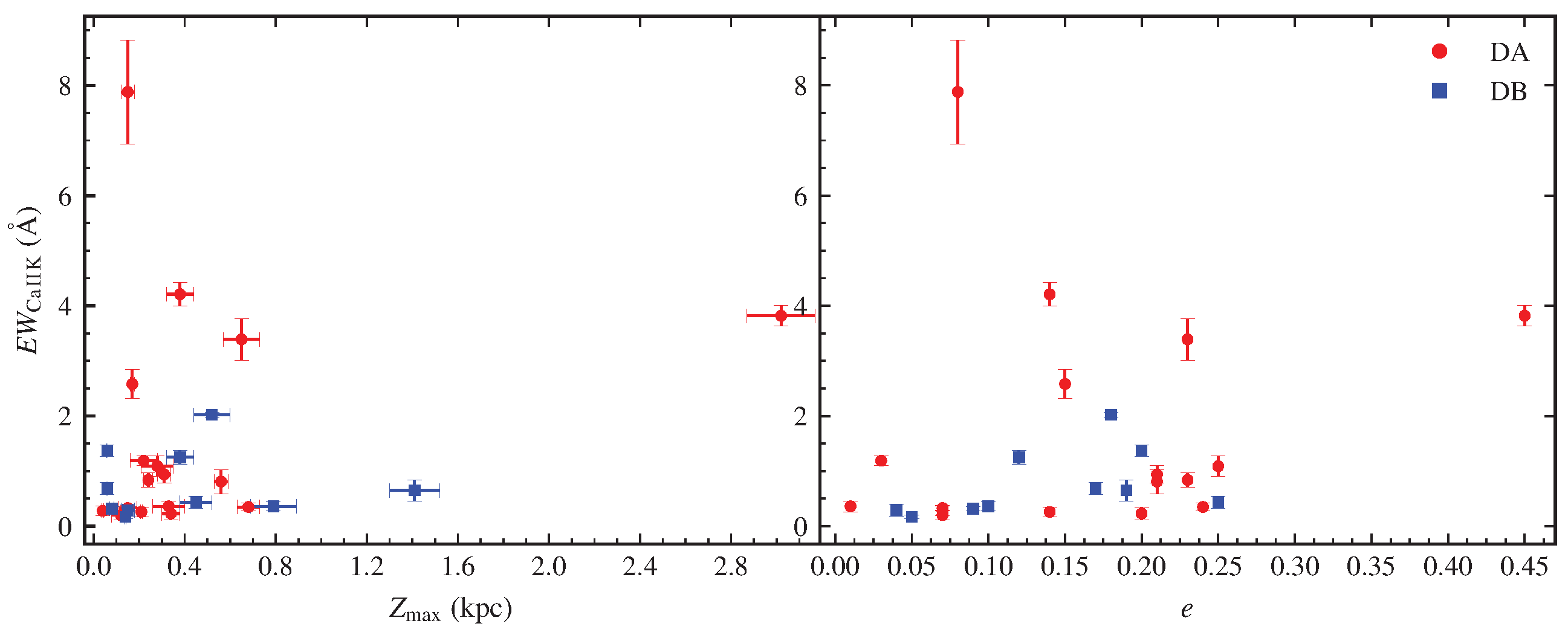
To explore a potential connection between the strength of metal pollution and kinematics, we encode the equivalent width of the Ca II K line (), as a color scale in Figure 5. The distribution of on the Toomre diagram does not show any significant differences between the Galactic populations of DA and DB white dwarfs. Figure 6 shows the distribution of DA and DB white dwarfs in the vs diagram and the vs. e diagram. We do not observe any significant differences in the distribution across these kinematic diagrams either. These results suggest that is largely independent of kinematic features, and that the strength of surface metal pollution in white dwarfs is primarily determined by the accretion history of their local planetary or minor-body systems, with only a weak connection to the large-scale Galactic dynamical environment. Consequently, metal pollution appears to be common across different disk components of the Galaxy, indicating ongoing or recurrent evolution of white dwarf planetary systems within various Galactic structures.
5. Conclusions
In this paper, by combining LAMOST DR9 and Gaia DR3 data, we performed spectral and kinematic analyses for 27 polluted white dwarfs (17 DA and 10 DB) selected from the catalog of polluted white dwarf candidates by Badenas-Agusti et al. [1]. We derived the effective temperature (), surface gravity (), and radial velocity (), measured the Ca II K line parameters ( and ), and inferred the cooling ages, as well as three-dimensional Galactic kinematics and orbital parameters. Based on these results, we draw the following conclusions:
- 1.
- We utilize the relationship between and derived from the sdB sample by Li et al. [27]. Our analysis shows that most of the targets lie above the pure-ISM expectation, indicating that for the majority of these objects, the Ca II K line does not originate from the ISM, which does not play a dominant role in the observed metal pollution of white dwarfs. By comparing the radial velocities (RV) of the white dwarf photospheric lines (H Balmer for DA-type and He I for DB-type) with the RV of the Ca II K line, we find that the Ca II K line is photospheric for 10 objects, while for 17 objects it originates externally, likely from circumstellar material (CSM).
- 2.
- In our sample of 27 metal-polluted white dwarfs, the versus effective temperature () diagram shows that DA-type white dwarfs exhibit relatively larger values in the temperature range –, while the line strength decreases markedly with increasing effective temperature, particularly for . This result is consistent with previous studies. The DB-type white dwarfs are mainly distributed in the region . At , helium lines disappear; therefore, a comprehensive investigation of the evolution of metal abundances in helium-dominated atmospheres requires the inclusion of DZ white dwarfs and larger samples. In the versus cooling age () diagram, DA white dwarfs span a wide range of cooling ages, from nearly zero up to about 4.0 Gyr. Relatively large values are mainly found in the cooling-age interval –1.4 Gyr, whereas fewer objects are present at other cooling ages. This distribution is likely influenced by sample selection effects. The DB white dwarfs in our sample are concentrated at Gyr, and their values show a trend of first increasing and then decreasing with cooling age. Notably, no statistically significant difference in the distributions between DA and DB white dwarfs is found in the overlapping cooling-age range of 0.0–0.5 Gyr. These behaviours can be explained by the interplay of convection zone evolution, metal settling (diffusion), and ongoing accretion of planetary debris [7,39,40].
- 3.
- Kinematic analysis of the distribution shows no significant differences between the Galactic populations of DA and DB white dwarfs. This suggests that the strength of surface metal pollution in white dwarfs is primarily determined by the accretion history of their local planetary or minor-body systems, with only a weak connection to the large-scale Galactic dynamical environment. Consequently, metal pollution is found to be common across different disk components of the Galaxy, indicating ongoing or recurrent evolution of white dwarf planetary systems within various Galactic structures.
The current sample size is modest and relies on LAMOST low-resolution spectra; thus, systematic uncertainties in velocities and equivalent widths () remain limited by the spectral resolution and signal-to-noise ratio (S/N). Future high-resolution and high-signal-to-noise spectroscopic observations will significantly improve the accuracy of metal-line measurements and further verify the conclusions of this study.
Acknowledgments
This work is supported by the National Natural Science Foundation of China (NSFC) under grants 12173028 and 12573035, the National Key R&D Program of China (Nos. 2021YFA1600401 and 2021YFA1600400), the Chinese Space Station Telescope project (CMS-CSST-2021-A10), and the Innovation Team Funds of China West Normal University (No. KCXTD2022-6). The Guoshoujing Telescope (the Large Sky Area Multi-Object Fiber Spectroscopic Telescope, LAMOST) is a National Major Scientific Project built by the Chinese Academy of Sciences. Funding for the project has been provided by the National Development and Reform Commission. LAMOST is operated and managed by the National Astronomical Observatories, Chinese Academy of Sciences. This work has made use of data from the European Space Agency (ESA) mission Gaia (https://www.cosmos.esa.int/gaia), processed by the Gaia Data Processing and Analysis Consortium (DPAC, https://www.cosmos.esa.int/web/gaia/dpac/consortium). Funding for the DPAC has been provided by national institutions, in particular the institutions participating in the Gaia Multilateral Agreement. Software used in this work includes astropy [48,49,50] and galpy [33].
Conflicts of Interest
The authors declare no conflicts of interest.
Appendix A. Parameter Measurement Results
In this appendix, we provide additional data supporting the main results of this study. Appendix Table A1 lists the measured atmospheric parameters, radial velocities, equivalent widths of the Ca line, radial velocities of the Ca line, and cooling ages for the 27 polluted white dwarfs analyzed in this work. Appendix Table A2 summarizes the Galactic kinematic parameters, including the three-dimensional space velocities and orbital properties derived from the available data.

Table A1.
Atmospheric Parameters of 27 Polluted White Dwarfs.
| No. | Gaia EDR3 ID | LAMOST obsID | Cooling | Total | |||||
|---|---|---|---|---|---|---|---|---|---|
| (K) | (cgs) | (km/s) | (km/s) | (Å) | (Gyr) | (Gyr) | |||
| Hydrogen-rich white dwarfs | |||||||||
| 1 | 1565012935076040832 | 564901178 | 7103±63 | 7.74±0.09 | 20.33±4.66 | – | |||
| 2 | 200924312484080256 | 302715031 | 21631±525 | 7.69±0.05 | – | ||||
| 3 | 2564020159166337024 | 472002174 | 6493±35 | 7.41±0.03 | – | ||||
| 4 | 2564945432560219008 | 354812027 | 7329±64 | 7.75±0.11 | – | ||||
| 5 | 2759588063311504768 | 355001148 | 6512±42 | 7.64±0.09 | – | ||||
| 6 | 333392060349558784 | 778504097 | 28989±405 | 8.20±0.07 | |||||
| 7 | 3360183783038606336 | 422409198 | 7850±44 | 7.31±0.07 | – | ||||
| 8 | 340886198462842112 | 854612056 | 6066±33 | 7.58±0.03 | – | ||||
| 9 | 3440707857129932672 | 185908034 | 7808±38 | 7.89±0.06 | |||||
| 10 | 3669065354086975872 | 812815099 | 7648±23 | 7.81±0.04 | |||||
| 11 | 480570075502703488 | 613507047 | 6617±42 | 8.27±0.08 | |||||
| 12 | 642549544391197440 | 713109166 | 11374±115 | 8.19±0.05 | |||||
| 13 | 716504796716020352 | 483112174 | 7374±20 | 7.96±0.03 | |||||
| 14 | 762684864901596928 | 620008163 | 26361±364 | 7.51±0.06 | – | ||||
| 15 | 917141857485288704 | 793608149 | 6820±23 | 7.43±0.07 | – | ||||
| 16 | 95297185335797120 | 378505204 | 7683±114 | 8.71±0.09 | |||||
| 17 | 994846611963848704 | 853011165 | 13018±582 | 7.99±0.12 | |||||
| Helium-rich white dwarfs | |||||||||
| 1 | 1032748903780398592 | 604516136 | 13662±171 | 8.06±0.11 | |||||
| 2 | 1196531988354226560 | 558410149 | 16121±120 | 7.95±0.06 | |||||
| 3 | 1527809271227078272 | 342506137 | 16323±110 | 7.90±0.06 | |||||
| 4 | 203931163247581184 | 295304028 | 18468±63 | 8.29±0.02 | |||||
| 5 | 3351139990665573120 | 387301118 | 16362±193 | 8.13±0.09 | |||||
| 6 | 3878793490528218752 | 868302211 | 21404±201 | 8.15±0.03 | |||||
| 7 | 4002914643768684288 | 629804063 | 14832±81 | 8.49±0.04 | |||||
| 8 | 5187830356195791488 | 837313013 | 15759±67 | 8.14±0.03 | |||||
| 9 | 689352219629097856 | 601709080 | 23046±134 | 7.87±0.02 | |||||
| 10 | 972551088836290816 | 632707021 | 14481±102 | 7.98±0.07 | |||||
Table A2.
Galactic Kinematic Parameters of 27 Polluted White Dwarfs.
| No. | Gaia EDR3 ID | LAMOST obsID | U | V | W | e | ||||
|---|---|---|---|---|---|---|---|---|---|---|
| (km/s) | (km/s) | (km/s) | kpc | kpc | kpc | km/s kpc | ||||
| Hydrogen-rich white dwarfs | ||||||||||
| 1 | 1565012935076040832 | 564901178 | -0.01 | -21.25 | 12.09 | 8.60 | 8.11 | 0.03 | 0.22 | 1.80 |
| 2 | 200924312484080256 | 302715031 | 33.91 | -9.24 | 6.55 | 10.67 | 8.06 | 0.14 | 0.21 | 1.22 |
| 3 | 2564020159166337024 | 472002174 | -21.68 | -4.98 | -3.05 | 9.81 | 8.37 | 0.08 | 0.15 | 0.66 |
| 4 | 2564945432560219008 | 354812027 | 0.18 | -68.74 | -56.77 | 8.48 | 5.35 | 0.23 | 0.65 | 13.21 |
| 5 | 2759588063311504768 | 355001148 | 56.72 | -53.07 | 7.97 | 9.39 | 5.64 | 0.25 | 0.28 | 2.37 |
| 6 | 333392060349558784 | 778504097 | -70.12 | -11.40 | -26.16 | 11.20 | 7.45 | 0.20 | 0.34 | 2.65 |
| 7 | 3360183783038606336 | 422409198 | -53.97 | -28.97 | 4.58 | 9.57 | 7.00 | 0.15 | 0.17 | 1.01 |
| 8 | 340886198462842112 | 854612056 | 5.04 | -70.87 | 9.36 | 8.67 | 5.39 | 0.23 | 0.24 | 2.11 |
| 9 | 3440707857129932672 | 185908034 | -12.57 | -35.75 | -4.23 | 8.48 | 7.38 | 0.07 | 0.04 | 0.05 |
| 10 | 3669065354086975872 | 812815099 | 19.90 | -10.72 | 15.64 | 9.76 | 8.04 | 0.01 | 0.33 | 3.15 |
| 11 | 480570075502703488 | 613507047 | 31.49 | -68.36 | -37.00 | 9.14 | 5.92 | 0.21 | 0.56 | 8.50 |
| 12 | 642549544391197440 | 713109166 | 5.09 | -33.96 | 2.98 | 8.60 | 7.40 | 0.07 | 0.15 | 0.84 |
| 13 | 716504796716020352 | 483112174 | -6.02 | -5.72 | -16.38 | 9.68 | 8.42 | 0.07 | 0.12 | 0.49 |
| 14 | 762684864901596928 | 620008163 | -86.49 | -7.18 | 19.56 | 12.08 | 7.48 | 0.24 | 0.68 | 8.59 |
| 15 | 917141857485288704 | 793608149 | -36.13 | 2.96 | 15.75 | 11.03 | 8.34 | 0.14 | 0.38 | 3.55 |
| 16 | 95297185335797120 | 378505204 | 59.76 | -126.12 | 94.56 | 9.25 | 3.55 | 0.45 | 3.02 | 163.06 |
| 17 | 994846611963848704 | 853011165 | -35.43 | -65.12 | -26.45 | 8.70 | 5.64 | 0.21 | 0.31 | 3.21 |
| Helium-rich white dwarfs | ||||||||||
| 1 | 1032748903780398592 | 604516136 | 49.09 | -27.13 | -66.61 | 10.47 | 7.16 | 0.19 | 1.41 | 34.40 |
| 2 | 1196531988354226560 | 558410149 | 29.09 | -6.13 | -28.37 | 10.28 | 8.06 | 0.12 | 0.38 | 3.74 |
| 3 | 1527809271227078272 | 342506137 | -58.32 | -66.08 | -33.68 | 8.93 | 5.40 | 0.25 | 0.45 | 6.40 |
| 4 | 203931163247581184 | 295304028 | -3.20 | -29.93 | -17.06 | 8.50 | 7.71 | 0.05 | 0.14 | 0.69 |
| 5 | 3351139990665573120 | 387301118 | 66.69 | 6.60 | -4.91 | 12.15 | 8.57 | 0.17 | 0.06 | 0.10 |
| 6 | 3878793490528218752 | 868302211 | -13.98 | -27.75 | -5.64 | 8.49 | 7.77 | 0.04 | 0.15 | 0.88 |
| 7 | 4002914643768684288 | 629804063 | -40.98 | -25.06 | -49.20 | 9.26 | 7.65 | 0.10 | 0.79 | 15.59 |
| 8 | 5187830356195791488 | 837313013 | 57.47 | 0.73 | 22.23 | 12.08 | 8.44 | 0.18 | 0.52 | 5.65 |
| 9 | 689352219629097856 | 601709080 | -5.97 | -41.20 | -6.03 | 8.51 | 7.12 | 0.09 | 0.08 | 0.27 |
| 10 | 972551088836290816 | 632707021 | -47.83 | -56.27 | -6.75 | 8.93 | 5.96 | 0.20 | 0.06 | 0.13 |
Appendix B. Fitting Diagram
In this appendix, we provide additional figures supporting the main results of this study. Figure A7 shows the spectral fitting plots for all targets, and Figure A8 presents the Ca line fitting plots.
Figure A7.
Spectral fitting plots for the 27 polluted white dwarfs. The first 17 targets are classified as DA-type white dwarfs, while the remaining 10 targets are DB-type white dwarfs. The black curves represent the LAMOST observed spectra, the red curves correspond to the best-fitting models, and the green dots indicate the residuals.
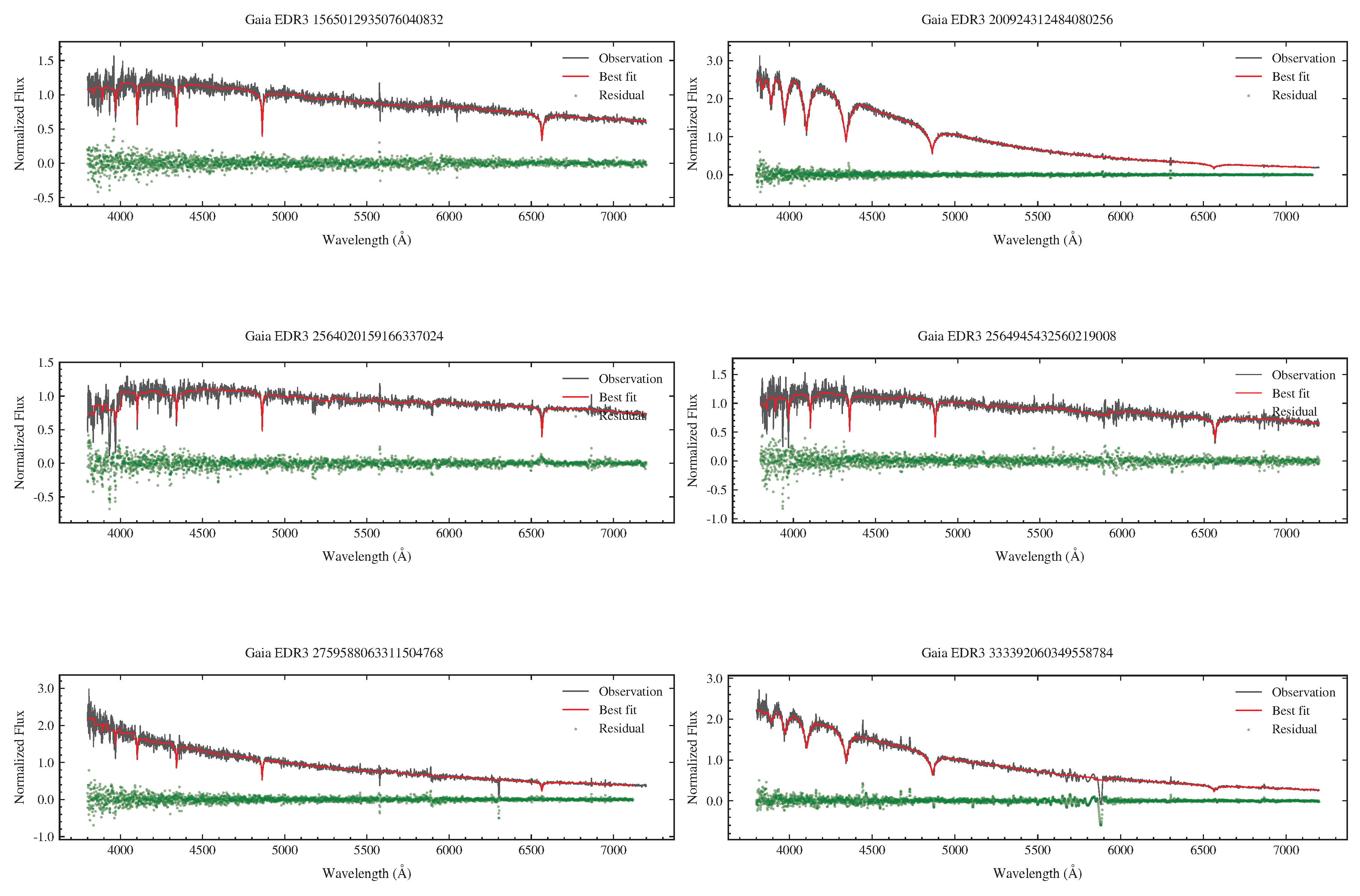
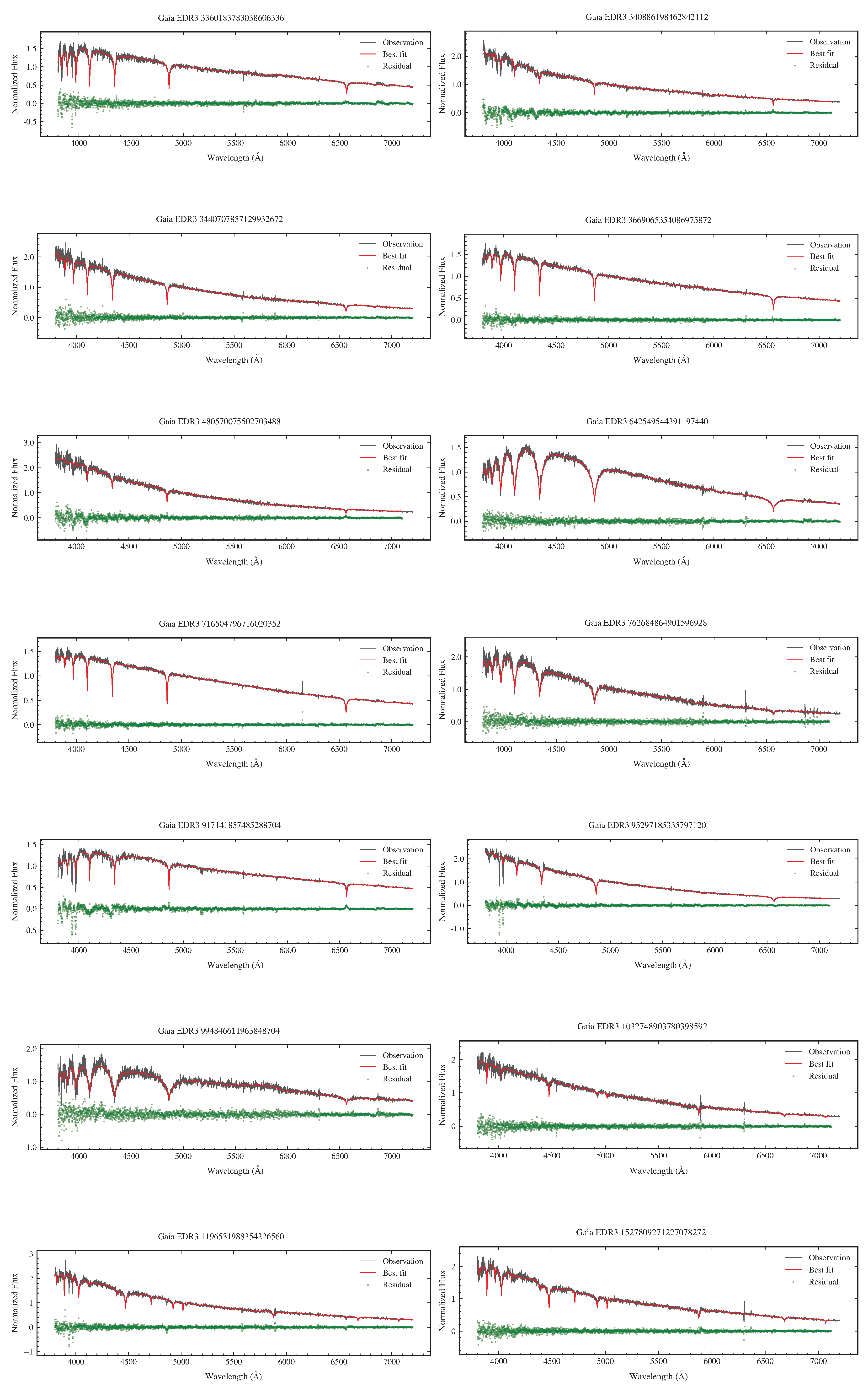
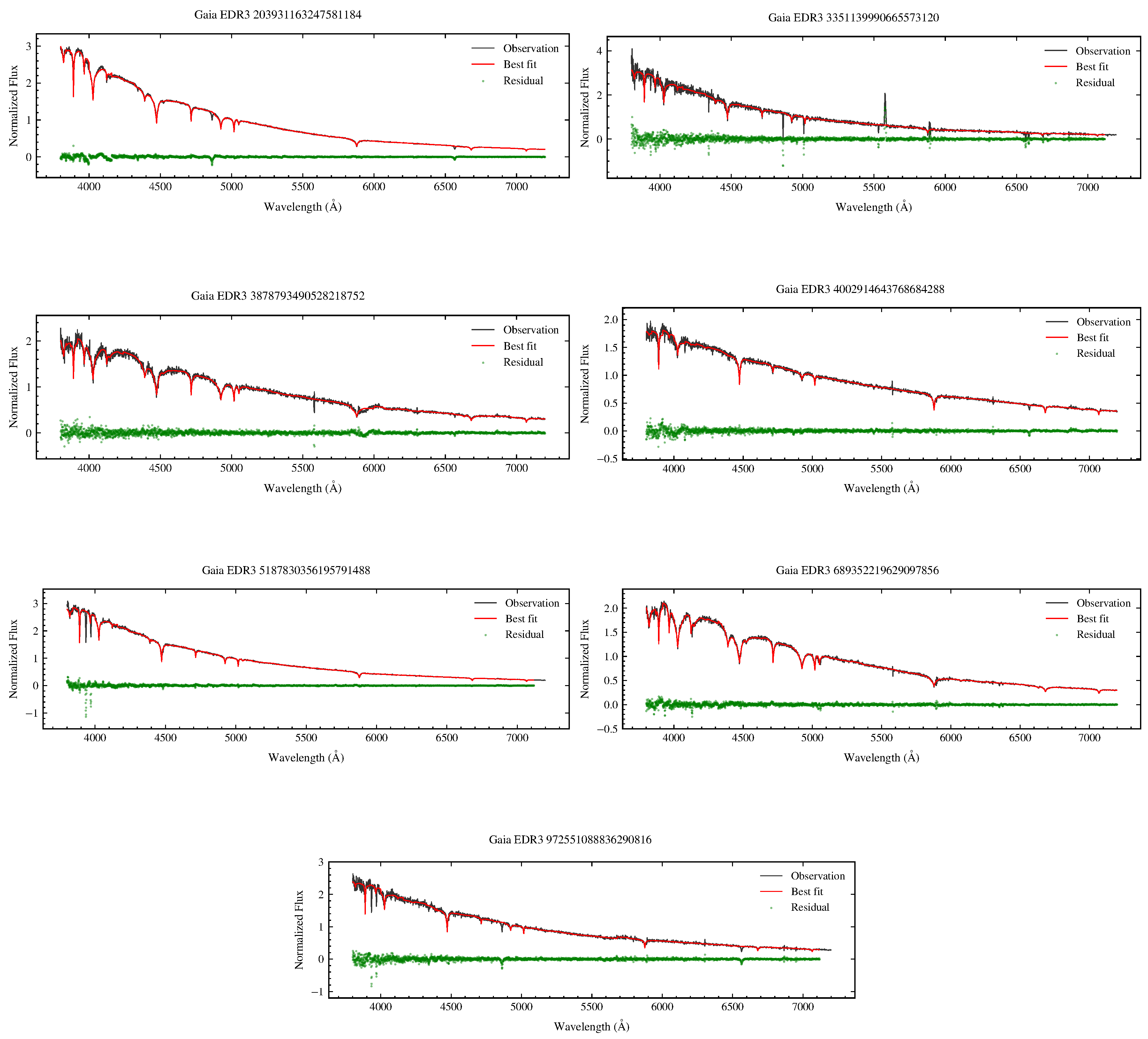
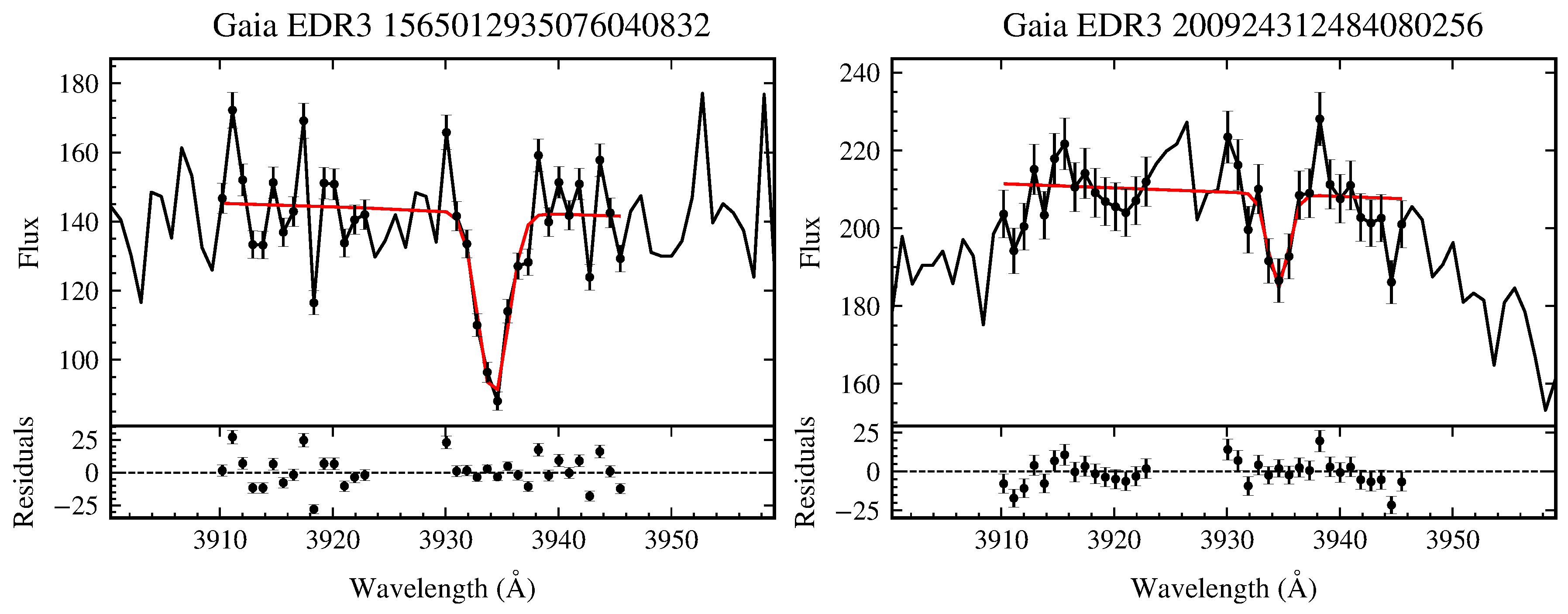
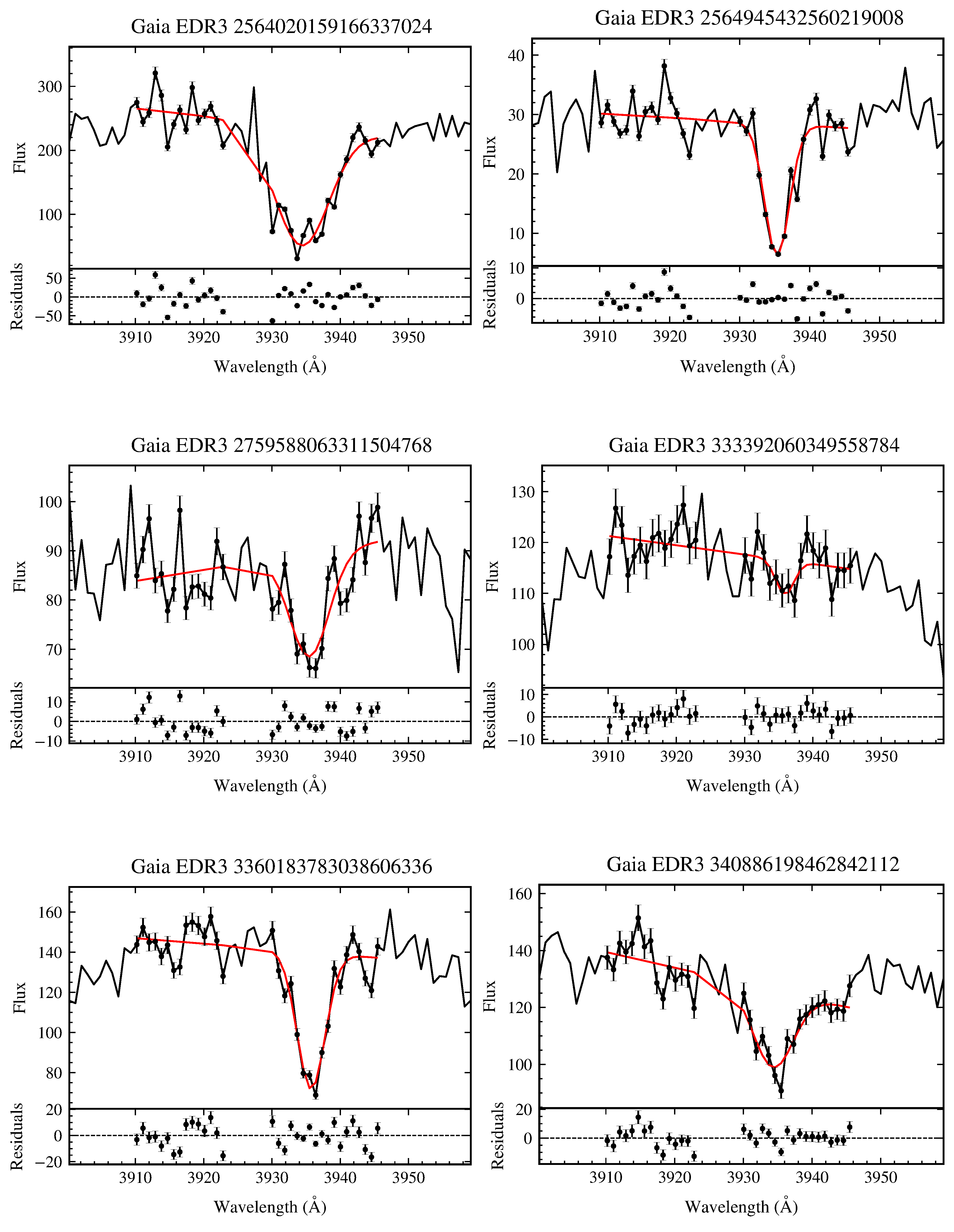
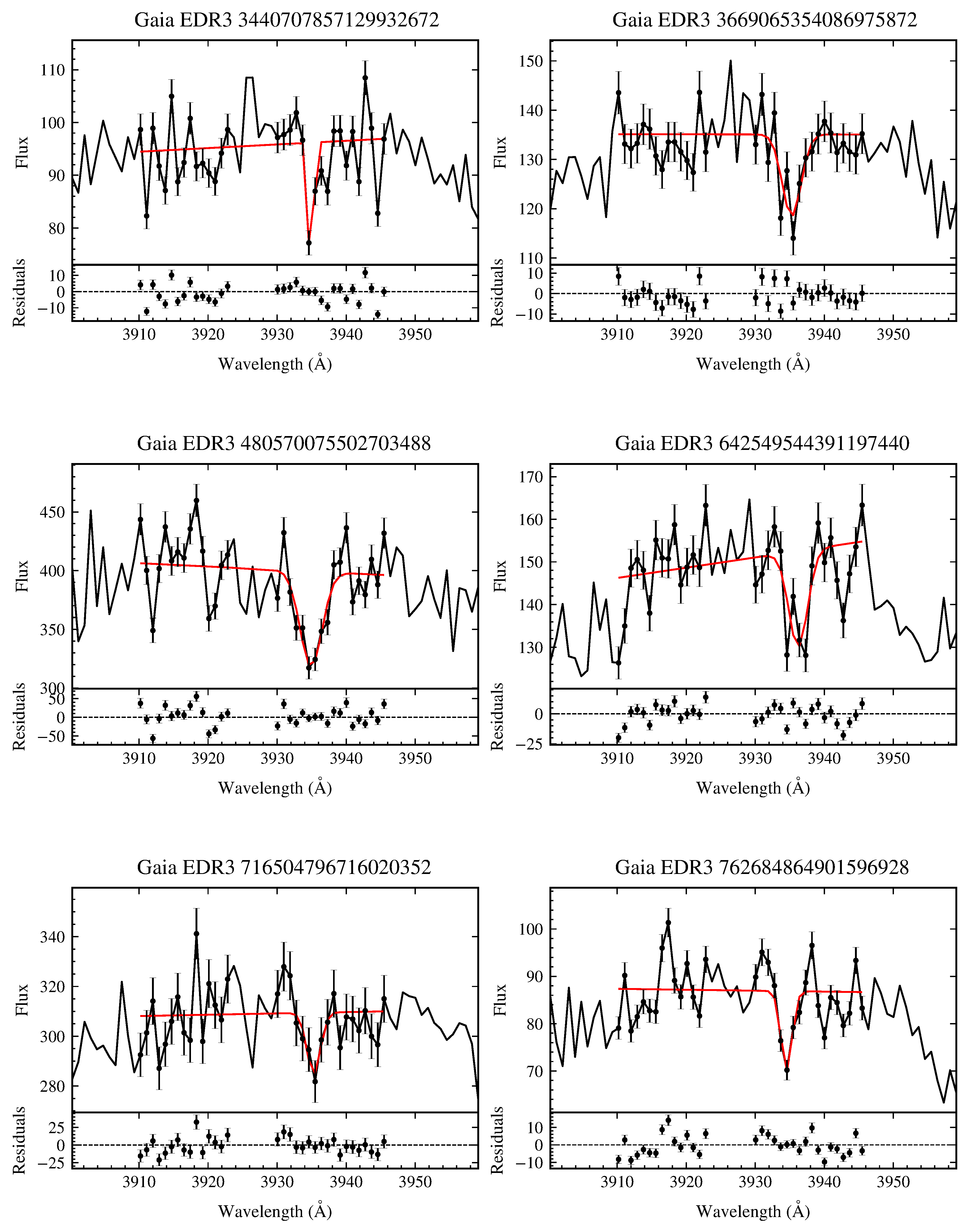
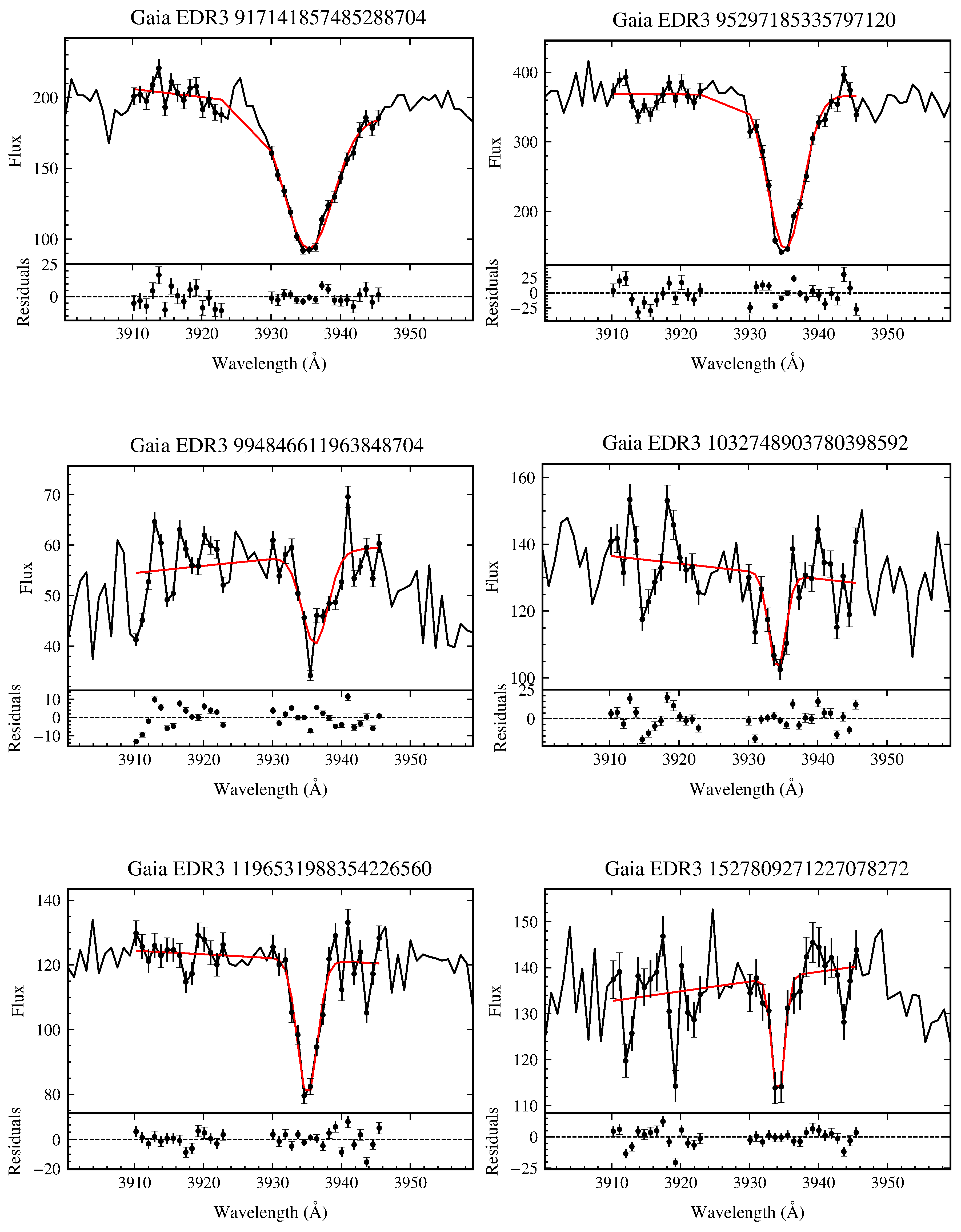
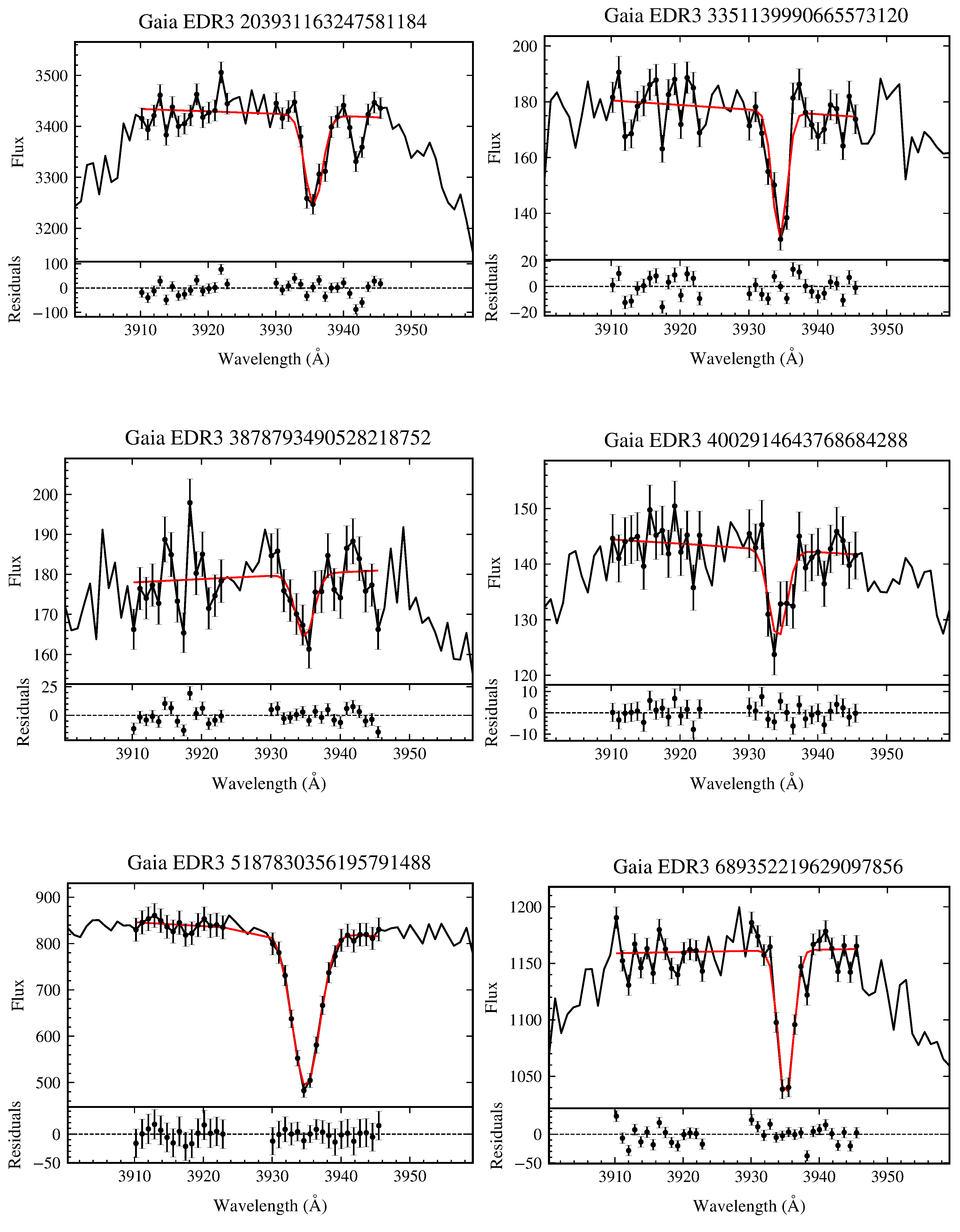
Figure A8.
Gaussian fitting results of the Ca II K line for 27 targets. Top panels: observed spectra in the wavelength range 3900–3960 Å; the black dots denote the data points used for the fitting, including the line core, line wings, and the local continuum. The red curves show the best-fitting Gaussian models. Bottom panels: fitting residuals, illustrating the differences between the data and the models.
| 1 | |
| 2 |
References
- Badenas-Agusti, M.; Vanderburg, A.; Blouin, S.; et al. MNRAS 2024, 527, 4515. [CrossRef]
- Podsiadlowski, P.; Han, Z.; Eggleton, P. P. AAS Meeting Abstracts 1993, 183, 101.05.
- Althaus, L. G.; Córsico, A. H.; Isern, J.; et al. A&ARv 2010, 18, 471. [CrossRef]
- Ferrario, L.; Wickramasinghe, D. T.; Liebert, J.; Williams, K. A. PASP 2001, 113, 409.
- Zuckerman, B.; Koester, D.; Reid, I. N.; et al. ApJ 2003, 596, 477. [CrossRef]
- Zuckerman, B.; Koester, D.; Melis, C.; et al. ApJ 2007, 671, 872. [CrossRef]
- Koester, D.; Gänsicke, B. T.; Farihi, J. A&A 2014, 566, A34. [CrossRef]
- Paquette, C.; Pelletier, C.; Fontaine, G.; et al. ApJS 1986, 61, 197. [CrossRef]
- Koester, D. 2009, A&A 498, 517. [CrossRef]
- Aannestad, P. A.; Sion, E. M. AJ 1985, 90, 1832. [CrossRef]
- Alcock, C.; Illarionov, A. ApJ 1980, 235, 534. [CrossRef]
- Jura, M.; Young, E. D. Annual Review of Earth and Planetary Sciences 2014, 42, 45. [CrossRef]
- Zuckerman, B.; Becklin, E. E. Nature 1987, 330, 138. [CrossRef]
- Jura, M. ApJL 2003, 584, L91. [CrossRef]
- Gänsicke, B. T.; Marsh, T. R.; Southworth, J.; et al. Science 2006, 314, 1908. [CrossRef] [PubMed]
- Cunningham, T.; Wheatley, P. J.; Tremblay, P.-E.; et al. Nature 2022, 602, 219. [CrossRef] [PubMed]
- Mullally, S. E.; Debes, J.; Cracraft, M.; et al. ApJL 2024, 962, L32. [CrossRef]
- Malamud, U. Encyclopedia of Astrophysics 2026, 1, 553. [CrossRef]
- Zhao, G.; Zhao, Y.-H.; Chu, Y.-Q.; et al. Research in Astronomy and Astrophysics 2012, 12, 723. [CrossRef]
- Yan, H.; Li, H.; Wang, S.; et al. The Innovation 2022, 3, 100224. [CrossRef]
- Prusti, T.; de Bruijne, J. H. J. Gaia Collaboration. A&A 2016, 595, A1. [Google Scholar] [CrossRef]
- Brown, A. G. A.; Vallenari, A. Gaia Collaboration; A&A, 2021; Volume 649, p. A1. [Google Scholar] [CrossRef]
- Koester, D. Memorie della Societa Astronomica Italiana 2010, 81, 921.
- Tremblay, P.-E.; Ludwig, H.-G.; Steffen, M.; et al. A&A 2013, 552, A13. [CrossRef]
- Cukanovaite, E.; Tremblay, P.-E.; Bergeron, P.; et al. MNRAS 2021, 501, 5274. [CrossRef]
- Cui, X.-Q.; Zhao, Y.-H.; Chu, Y.-Q.; et al. Research in Astronomy and Astrophysics 2012, 12, 1197. [CrossRef]
- Li, J.; Wolf, C.; Li, J.; et al. MNRAS 2025, 537, 1950. [CrossRef]
- Liu, C.; Cui, W.-Y.; Zhang, B.; et al. Research in Astronomy and Astrophysics 2015, 15, 1137. [CrossRef]
- Kiman, R.; Xu, S.; Faherty, J. K.; et al. AJ 2022, 164, 62. [CrossRef]
- Bédard, A.; Bergeron, P.; Brassard, P.; et al. ApJ 2020, 901, 93. [CrossRef]
- Lallement, R.; Vergely, J.-L.; Valette, B.; et al. A&A 2014, 561, A91. [CrossRef]
- Schönrich, R.; Binney, J.; Dehnen, W. MNRAS 2010, 403, 1829. [CrossRef]
- Bovy, J. ApJS 2015, 216, 29. [CrossRef]
- Green, G. M.; Schlafly, E.; Zucker, C.; et al. ApJ 2019, 887, 93. [CrossRef]
- Schlafly, E. F.; Finkbeiner, D. P. ApJ 2011, 737, 103. [CrossRef]
- Megier, A.; Strobel, A.; Galazutdinov, G. A.; et al. A&A 2009, 507, 833. [CrossRef]
- Zuckerman, B.; Melis, C.; Klein, B.; et al. ApJ 2010, 722, 725. [CrossRef]
- Coutu, S.; Dufour, P.; Bergeron, P.; et al. ApJ 2019, 885, 74. [CrossRef]
- Dupuis, J.; Fontaine, G.; Wesemael, F. ApJS 1993, 87, 345. [CrossRef]
- Zhu, C.; Liu, H.; Wang, Z.; et al. A&A 2021, 654, A57. [CrossRef]
- Blouin, S.; Xu, S. MNRAS 2022, 510, 1059. [CrossRef]
- Farihi, J. New Astronomy Reviews 2016, 71, 9. [CrossRef]
- Bonsor, A.; Mustill, A. J.; Wyatt, M. C. MNRAS 2011, 414, 930. [CrossRef]
- Bédard, A. Ap&SS 2024, 369, 43. [CrossRef]
- Williams, J. T.; Gänsicke, B. T.; Swan, A.; et al. A&A 2024, 691, A352. [CrossRef]
- Cunningham, T.; Tremblay, P.-E.; O’Brien, M.; et al. MNRAS 2025, 539. [CrossRef]
- Torres, S.; Cantero, C.; Rebassa-Mansergas, A.; et al. MNRAS 2019, 485, 5573. [CrossRef]
- Robitaille, T. P.; Tollerud, E. J. Astropy Collaboration; A&A, 2013; Volume 558, p. A33. [Google Scholar] [CrossRef]
- Price-Whelan, A. M.; Sipocz, B. M. Astropy Collaboration. AJ 2018, 156, 123. [Google Scholar] [CrossRef]
- Price-Whelan, A. M.; Lim, P. L. Astropy Collaboration. ApJ 2022, 935, 167. [Google Scholar] [CrossRef]
Figure 1.
Correlation between and for 27 polluted white dwarfs. Error bars represent the measurement uncertainties. Red and blue points represent DA and DB types, respectively. The black dashed line shows the best-fitting ISM relationship from Li et al. [27], with the gray shaded region indicating its 95% confidence interval.
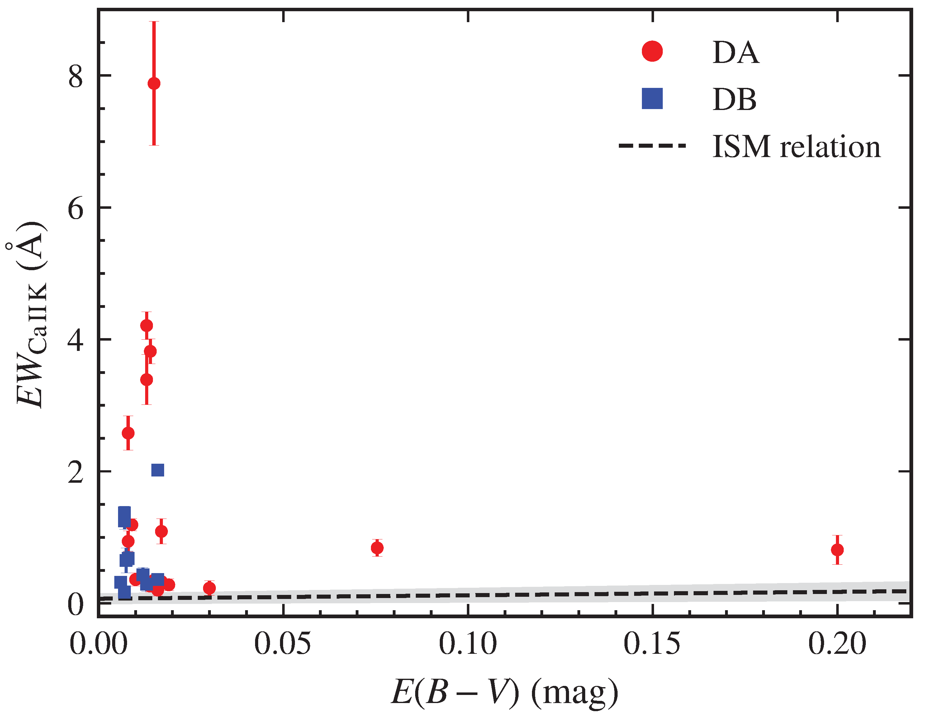
Figure 2.
Distribution of the Ca equivalent width () and the velocity offset () diagram. Here, , where is derived from the H Balmer lines for DA stars and from He I lines for DB stars. The dashed lines indicate the threshold .
Figure 2.
Distribution of the Ca equivalent width () and the velocity offset () diagram. Here, , where is derived from the H Balmer lines for DA stars and from He I lines for DB stars. The dashed lines indicate the threshold .
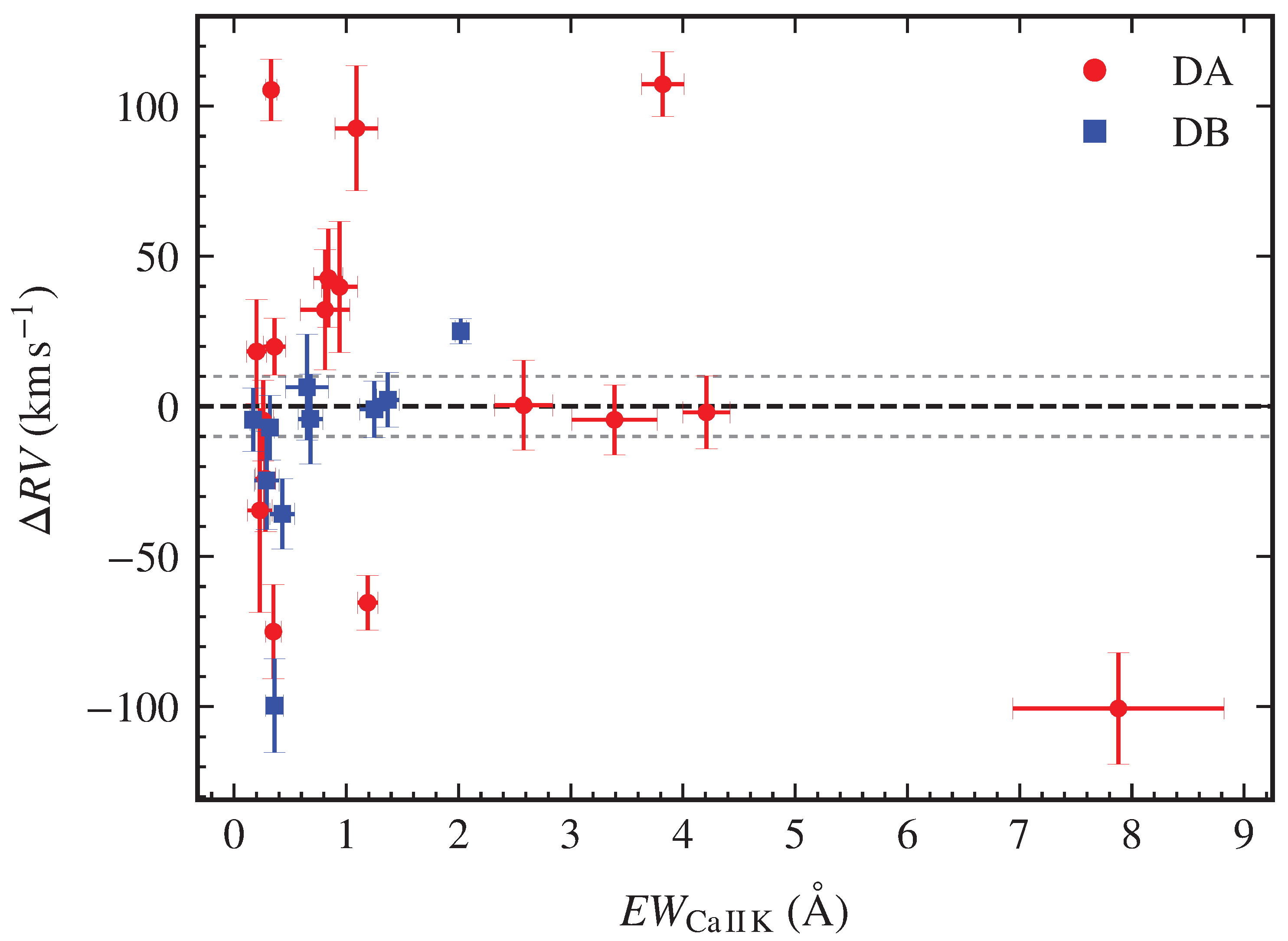
Figure 3.
Distribution of the Ca II K equivalent width () with effective temperature for 27 polluted white dwarfs. Red points represent DA white dwarfs, and blue points represent DB white dwarfs. Error bars indicate measurement uncertainties.
Figure 3.
Distribution of the Ca II K equivalent width () with effective temperature for 27 polluted white dwarfs. Red points represent DA white dwarfs, and blue points represent DB white dwarfs. Error bars indicate measurement uncertainties.
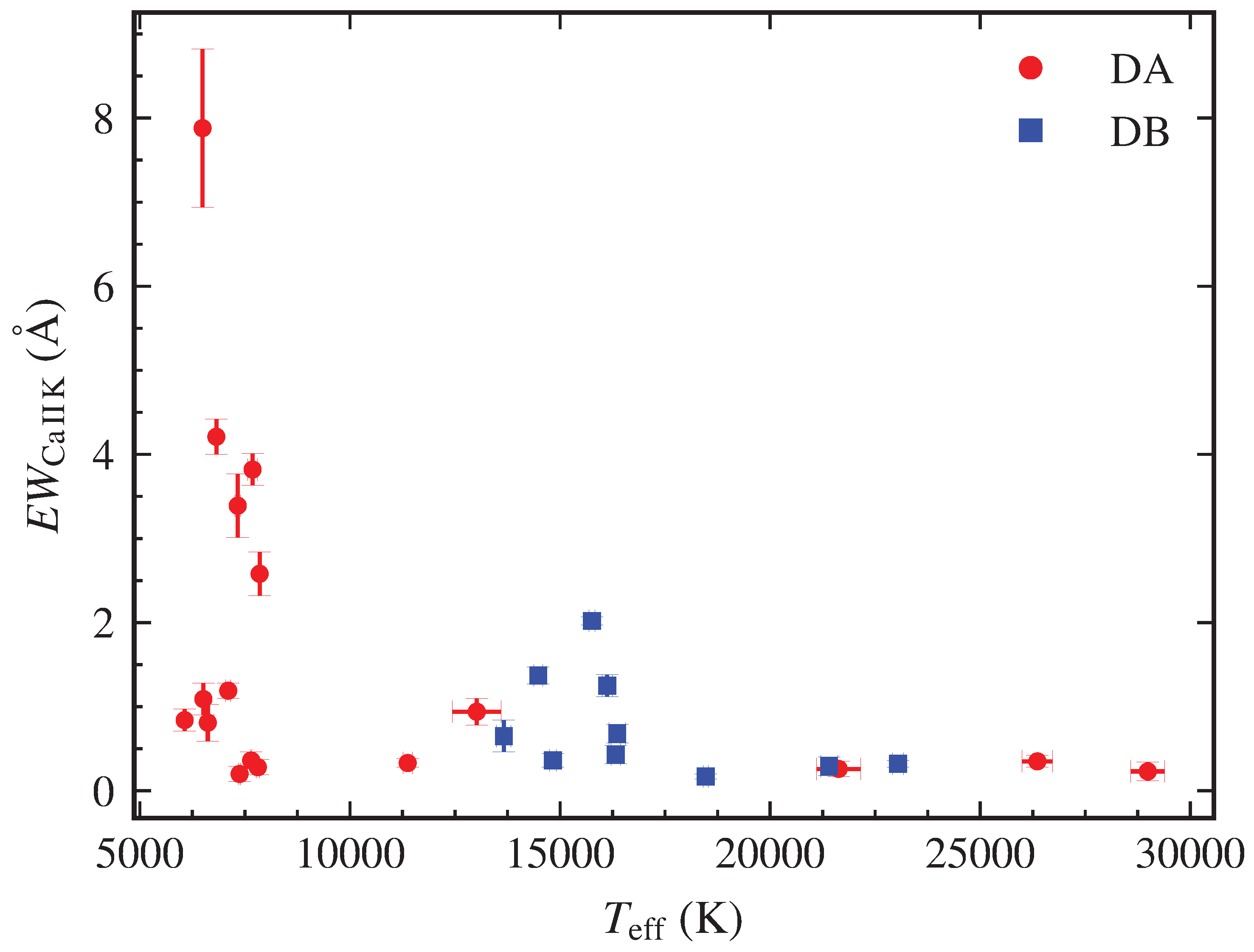
Figure 4.
Distribution of the Ca II K equivalent width () versus cooling age () for 27 polluted white dwarfs. Red and blue points denote DA and DB white dwarfs, respectively; error bars indicate measurement uncertainties.
Figure 4.
Distribution of the Ca II K equivalent width () versus cooling age () for 27 polluted white dwarfs. Red and blue points denote DA and DB white dwarfs, respectively; error bars indicate measurement uncertainties.
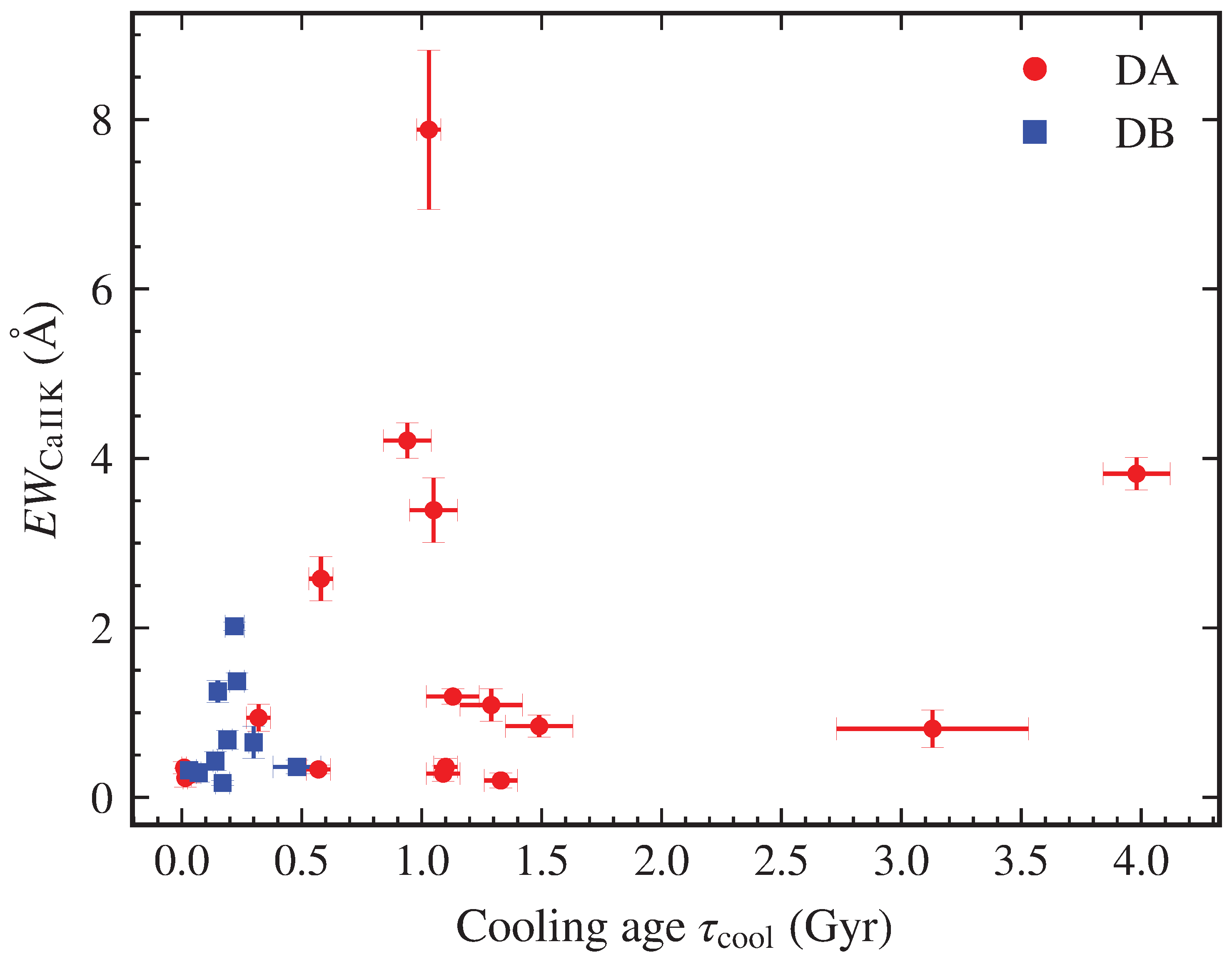
Figure 5.
Toomre diagrams for the 27 polluted white dwarfs before and after correcting for gravitational redshift. Circles and squares represent DA and DB white dwarfs, respectively, with the point color indicating the equivalent width of the Ca II K line (). The upper (lower) panel shows the results based on the observed radial velocities without (with) correction for gravitational redshift. The dashed ellipses mark the and velocity boundaries of the thin-disk population, as defined by Torres et al. [47].
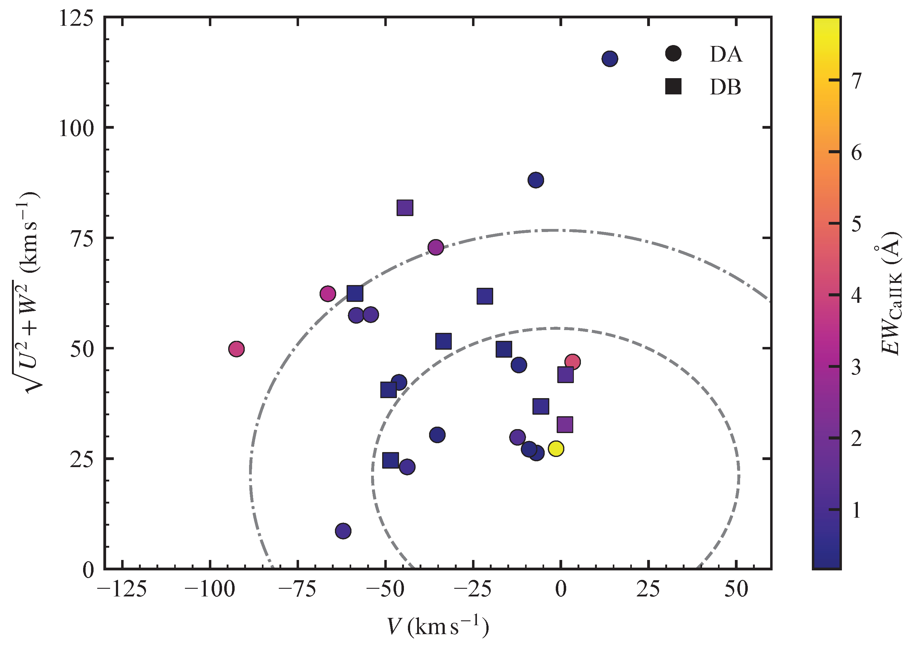
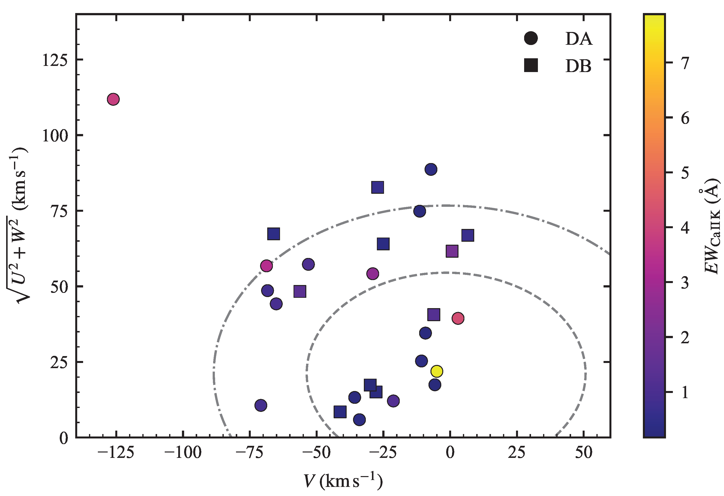
Figure 6.
The distribution of 27 polluted white dwarfs in the Ca II K line equivalent width () versus the maximum vertical height of the orbit above the Galactic plane () diagram (left), and versus eccentricity (e) diagram (right). Red circles and blue squares represent DA and DB white dwarfs, respectively.
Disclaimer/Publisher’s Note: The statements, opinions and data contained in all publications are solely those of the individual author(s) and contributor(s) and not of MDPI and/or the editor(s). MDPI and/or the editor(s) disclaim responsibility for any injury to people or property resulting from any ideas, methods, instructions or products referred to in the content. |
© 2026 by the authors. Licensee MDPI, Basel, Switzerland. This article is an open access article distributed under the terms and conditions of the Creative Commons Attribution (CC BY) license (http://creativecommons.org/licenses/by/4.0/).
Copyright: This open access article is published under a Creative Commons CC BY 4.0 license, which permit the free download, distribution, and reuse, provided that the author and preprint are cited in any reuse.


