Notes on Number Theory

1. Introduction

Modern number theory is shaped by two complementary viewpoints: the algebraic study of field extensions and their arithmetic invariants, and the analytic study of zeta and L-functions encoding prime-distribution phenomena. Cyclotomic fields remain the most explicit and historically influential class of number fields, yet many of the mechanisms they reveal—integral bases, ideal factorization, local ramification, and Frobenius elements—reappear throughout contemporary arithmetic, notably in the theory of elliptic curves and automorphic L-functions.

In this paper we develop a unified account of these themes. We begin with finite extensions $K/\mathbb{Q}$ and emphasize a concrete linear-algebraic realization: choosing a $\mathbb{Q}$-basis identifies K with a commutative subalgebra of $M_n\left(\mathbb{Q}\right)$, from which trace, norm, and discriminant arise naturally and can be reinterpreted through embeddings into $\overline{\mathbb{Q}}$[14,19]. This viewpoint leads to the ring of integers ${\mathcal{O}}_K$, Dedekind’s ideal factorization, and the class group as a quantitative measure of the deviation from unique factorization [7,19].

Cyclotomic fields $\mathbb{Q}\left({\zeta }_m\right)$ then provide a guiding family where these constructions can be made explicit. They connect classical problems—constructible polygons and reciprocity laws—to the description of abelian extensions of $\mathbb{Q}$ via the Kronecker–Weber theorem and its p-adic refinements [20,27]. Beyond their intrinsic interest, cyclotomic examples supply a laboratory for understanding how global arithmetic data are controlled by local behavior at primes.

To make the local–global principle transparent, we review Hilbert’s ramification theory and the decomposition of prime ideals in extensions. Decomposition and inertia groups, discriminants, and Frobenius elements organize the splitting of primes and foreshadow the Euler factors that appear in zeta and L-functions [10,19]. This sets the stage for the arithmetic-geometric side of the paper: elliptic curves over number fields, their group law, reduction at primes, and the associated Hasse–Weil L-function [23,24]. In this context, local factors, conductors, and Frobenius traces link algebraic structure to analytic behavior and motivate the Birch and Swinnerton-Dyer conjecture.

Finally, we include a collection of examples illustrating how integral transforms provide a common operational language across seemingly distant areas. In particular, the Laplace and Mellin transforms simultaneously linearize fractional operators and encode Dirichlet series; this perspective clarifies parallels between convolution algebras in fractional calculus and multiplicative structures in analytic number theory [10,16]. These examples suggest further directions where transform methods may inform arithmetic questions.

This paper continues as follows. Section 2 develops the algebraic and arithmetic foundations of number fields, including matrix realizations, rings of integers, embeddings, ideals, and class groups. Section 3 specializes to cyclotomic fields and their basic Galois and arithmetic properties. Section 4 presents ramification theory from the ideal-theoretic and Galois-theoretic viewpoints. Section 5 turns to elliptic curves and L-functions, emphasizing the interaction between reduction data and global invariants. Section 6 collects examples and cross-connections (including the transform-based viewpoint linking fractional calculus and number theory). Section 7 concludes with a brief summary and perspectives for further work.

2. Algebraic Extensions of Fields

We will examine finite extensions of the field of rational numbers, these are algebraic number fields. The cyclotomic fields are discussed due to the important role they play in the development of number theory. Gauss used cyclotomic fields to solve the problem of constructing a regular n-gon with compass and straightedge. In the mid-19th century, Kummer, working on Fermat’s Last Theorem and the Laws of Reciprocity, discovered a connection between the arithmetic of cyclotomic fields and the values of the Riemann $\zeta$ function at odd negative values of the argument. At the same time, in the mid-19th century, Kronecker formulated and partially proved a theorem classifying the abelian extensions of $\mathbb{Q}$. Thus, all extensions of $\mathbb{Q}$ with a commutative Galois group turn out to be cyclotomic fields and their subfields. The theorem of Kronecker, today known as the Kronecker-Weber theorem, was fully proved by Hilbert at the end of the 19th century. At the beginning of the 20th century, Kurt Hensel introduced p-adic numbers, leading to the emergence of the ring ${\mathbb{Z}}_p$ of p-adic integers and the field ${\mathbb{Q}}_p$ of p-adic rational numbers. This enabled the generalization of the theory of cyclotomic fields to reach p-adic cyclotomic extensions of ${\mathbb{Q}}_p$. In the 1960s, Iwasawa developed the theory of p-adic cyclotomic fields, which was used by Wiles in the proof of Fermat’s Last Theorem. Our goal will be to provide an overview of the classical theory of cyclotomic extensions.

2.1. Algebraic Number Fields as Matrix Algebras

Let $K/\mathbb{Q}$ be a finite extension, hence it is algebraic and separable ($\mathrm{char}\mathbb{Q}=0$). The primitive element theorem holds for finite separable extensions, hence $\exists \theta \in K:K=\mathbb{Q}\left(\theta \right)$. The map $\psi :\mathbb{Q}\left[x\right]\to \mathbb{Q}\left[\theta \right],f\mapsto f\left(\theta \right)$ is a surjective ring homomorphism, with kernel $\mathsf{Ker}\psi =\left(p_{\theta }\right)$, where $p_{\theta }$ is the minimal polynomial of $\theta$ over $\mathbb{Q}$. Since $p_{\theta }$ is irreducible over $\mathbb{Q}$, the ideal $\left(p_{\theta }\right)⊲\mathbb{Q}\left[x\right]$ is prime. The map $\mathbb{Q}\left[x\right]\to \mathbb{Z},f\mapsto deg\left(f\right)$ is a Euclidean function, therefore in $\mathbb{Q}\left[x\right]$ the division algorithm holds, and every ideal in $\mathbb{Q}\left[x\right]$ is principal. In particular, every nonzero prime ideal in $\mathbb{Q}\left[x\right]$ is principal and therefore maximal. Thus $\left(p_{\theta }\right)⊲\mathbb{Q}\left[x\right]$ is maximal, from which the factor ring $\mathbb{Q}\left[x\right]/\left(p_{\theta }\right)$ is a field. The homomorphism theorem gives a ring isomorphism $\mathbb{Q}\left[x\right]/\left(p_{\theta }\right)\cong \mathbb{Q}\left[\theta \right]$, which is an isomorphism of fields and $\mathbb{Q}\left[\theta \right]\equiv \mathbb{Q}\left(\theta \right)=K$. This isomorphism at $n=deg\left(p_{\theta }\right)$ shows that K is an n-dimensional vector space over $\mathbb{Q}$. Since $\theta$ does not satisfy a polynomial equation over $\mathbb{Q}$ of degree less than n, the elements $1,\theta ,\dots ,{\theta }^{n-1}$ are linearly independent over $\mathbb{Q}$ and therefore form a basis for $K/\mathbb{Q}$, from which $K={⨁}_{j=0}^{n-1}\mathbb{Q}{\theta }^j$.

We have obtained that K is a finite commutative $\mathbb{Q}$ algebra and thus is realized as a matrix subalgebra of $M_n\left(\mathbb{Q}\right)$. The realization is as follows: let us fix a basis $1,\theta ,\dots ,{\theta }^{n-1}$ for $K/\mathbb{Q}$ and define $h\in {\mathrm{Hom}}_{\mathbb{Q}}\left(K,{\mathrm{E}\mathrm{n}\mathrm{d}}_{\mathbb{Q}}K\right)$ where $h\left(\alpha \right)={\phi }_{\alpha }\in {\mathrm{E}\mathrm{n}\mathrm{d}}_{\mathbb{Q}}K$ with ${\phi }_{\alpha }\left(x\right)=\alpha x,\alpha ,x\in K$. We transition to matrix language: let $h^{\prime }\in \mathrm{H}\mathrm{o}\mathrm{m}\left({\mathrm{E}\mathrm{n}\mathrm{d}}_{\mathbb{Q}}K,M_n\left(\mathbb{Q}\right)\right),h^{\prime }\left({\phi }_{\alpha }\right)=A_{\alpha }$, associating with the operator its matrix in the fixed basis. If $p_{\theta }\left(x\right)=x^n+a_1{x}^{n-1}+\dots +a_n$ and $\alpha ={\sum }_{j=0}^{n-1}{c}_j{\theta }^j$, then $A_{\alpha }=(h^{\prime }\circ h)\left(\alpha \right)={\sum }_{j=0}^{n-1}{c}_j{A}_{\theta }^j$. The realization of K as a matrix algebra allows us to define two invariants of the extension $K/\mathbb{Q}$, trace and norm: ${\mathrm{T}\mathrm{r}}_{K/\mathbb{Q}}\in {\mathrm{H}\mathrm{o}\mathrm{m}}_{\mathbb{Q}}\left(K,\mathbb{Q}\right)N_{K/\mathbb{Q}}\in \mathrm{H}\mathrm{o}\mathrm{m}\left(K^{*},{\mathbb{Q}}^{*}\right)$, defined by ${\mathrm{Tr}}_{K/\mathbb{Q}}\left(\alpha \right)=\mathrm{Tr}{A}_{\alpha }$ and $N_{K/\mathbb{Q}}\left(\alpha \right)=\det A_{\alpha }$. The matrix $A_{\theta }$ is of the form:

$$A_{\theta }=\left(\begin{array}{cccccc}0& 0& 0& \dots & 0& -a_n\\ 1& 0& 0& \dots & 0& -a_{n-1}\\ 0& 1& 0& \dots & 0& -a_{n-2}\\ ⋮& ⋮& ⋮& & ⋮& ⋮\\ 0& 0& 0& \dots & 0& -a_2\\ 0& 0& 0& \dots & 1& -a_1\end{array}\right)$$

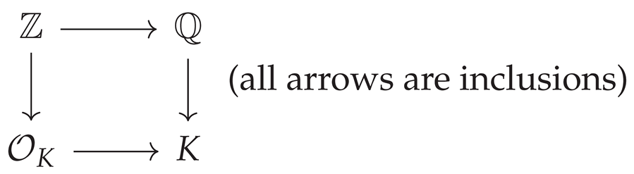
2.2. Ring of Integral Algebraic Numbers of a Number Field

An element $\alpha \in K$ is called integral (an integral algebraic number) if its minimal polynomial over $\mathbb{Q}$ has integer coefficients. Equivalently, $\alpha \in K$ is integral if its characteristic polynomial $f_{\alpha }\left(x\right)=\det \left(x{\mathbf{I}}_n-A_{\alpha }\right)$ has integer coefficients. The set of integral elements of K is denoted by ${\mathcal{O}}_K$ and is a ring with respect to the operations in K, according to the properties of integral extensions of rings. Schematically - the notation is as follows:

The properties of the ring of integers ${\mathcal{O}}_K$ of K are as follows: the field of fractions of ${\mathcal{O}}_K$ coincides with K. The ring ${\mathcal{O}}_K$ is integrally closed in K and is a free $\mathbb{Z}$ module of rank $n=[K:\mathbb{Q}]$, i.e., $\exists {\omega }_1,{\omega }_2,\dots ,{\omega }_n\in {\mathcal{O}}_K:{\mathcal{O}}_K={⨁}_{k=1}^n\mathbb{Z}{\omega }_k$. Every element $\alpha \in K$ can be represented in the form $\alpha ={\displaystyle \frac{a}{b}},a\in {\mathcal{O}}_K,b\in \mathbb{Z}$, therefore K has an ${\mathcal{O}}_K$ basis over $\mathbb{Q}$, i.e., $K={⨁}_{k=1}^n\mathbb{Q}{\omega }_k,{\omega }_k\in {\mathcal{O}}_K$. In particular, the primitive element $\theta$ of the extension $K/\mathbb{Q}$ can be chosen from ${\mathcal{O}}_K$ and from now on we will assume that we have chosen it in this way. We move on to defining the third invariant for the extension $K/\mathbb{Q}$. The mapping $K\times K\to \mathbb{Q},(\alpha ,\beta )\mapsto {\mathrm{Tr}}_{K/\mathbb{Q}}\left(\alpha \beta \right)$ is a non-degenerate symmetric bilinear form. We fix a basis ${\omega }_1,{\omega }_2,\dots ,{\omega }_n\in {\mathcal{O}}_K$ for $K/\mathbb{Q}$, and we set $d({\omega }_1,{\omega }_2,\dots ,{\omega }_n)=\det {\left({\mathrm{Tr}}_{K/\mathbb{Q}}\left({\omega }_i{\omega }_j\right)\right)}_{n\times n}$. The number $d({\omega }_1,{\omega }_2,\dots ,{\omega }_n)$ does not depend on the specific choice of basis and therefore is an invariant of the field K, which is denoted by $d_K$ and the equality $d_K=\mathrm{d}\mathrm{i}\mathrm{s}\mathrm{c}\left(p_{\theta }\right)$ holds. The importance of this invariant is expressed in the control of the decomposition of the prime numbers $p\in \mathbb{Z}$ into a product of prime ideals in ${\mathcal{O}}_K$, i.e., if the ideal $\left(p\right)⊲{\mathcal{O}}_K$ has a decomposition $\left(p\right)={\mathfrak{p}}_1^{e_1}\dots {\mathfrak{p}}_r^{e_r}$ of prime ideals ${\mathfrak{p}}_i⊲{\mathcal{O}}_K$, then $e_1=\dots =e_r=1$ if $p\nmid d_K$. If $p|d_K$, then $max\{e_1,\dots ,e_r\}\ge 2$. The control of the decomposition of prime numbers into a product of prime ideals in the ring of integers of an algebraic number field motivated Hilbert at the end of the 19th century to create ”Ramification theory”, which we will describe next.

2.3. Description of the Invariants of a Number Field Through Embeddings

Let $\overline{\mathbb{Q}}$ be the algebraic closure of $\mathbb{Q}$ and let $K=\mathbb{Q}\left(\theta \right)$. Any injective homomorphism $\sigma \in {Hom}_{\mathbb{Q}}(K,\overline{\mathbb{Q}})$ is called an embedding of K over $\mathbb{Q}$. The number of all such embeddings is $deg\left(p_{\theta }\right)=[K:\mathbb{Q}]=n$, because each embedding $\sigma$ is uniquely determined by its action on $\theta$, whereby considering $0=\sigma \left(0\right)=\sigma \circ p_{\theta }\left(\theta \right)=p_{\theta }\left(\sigma \left(\theta \right)\right)$ we conclude that $\sigma \left(\theta \right)$ is among the distinct roots of $p_{\theta }$, exactly n in number. Let S denote the set of these n embeddings. The invariants ${\mathrm{Tr}}_{K/\mathbb{Q}},N_{K/\mathbb{Q}},d_K$ of $K/\mathbb{Q}$ are described through embeddings: for any $\alpha \in K$ it holds:

$${\mathrm{Tr}}_{K/\mathbb{Q}}\left(\alpha \right)=\sum _{\sigma \in S}\sigma \left(\alpha \right),N_{K/\mathbb{Q}}\left(\alpha \right)=\prod _{\sigma \in S}\sigma \left(\alpha \right),d_K=\det {\left({\sigma }_i{\theta }^j\right)}_{i,j=0}^{n-1},f_{\alpha }\left(x\right)=\prod _{\sigma \in S}(x-\sigma \left(\alpha \right)).$$

The relationship between ${\mathcal{O}}_K$ and $\mathbb{Z}$ is mediated by ${\mathrm{Tr}}_{K/\mathbb{Q}},N_{K/\mathbb{Q}},d_K$, because $d_K\in \mathbb{Z}$ and the restrictions satisfy: ${\mathrm{Tr}}_{K/\mathbb{Q}}{|}_{{\mathcal{O}}_K}\in \mathrm{Hom}({\mathcal{O}}_K,\mathbb{Z})$ and $N_{K/\mathbb{Q}}{|}_{{\mathcal{O}}_K^{*}}\in \mathrm{Hom}({\mathcal{O}}_K^{*},{\mathbb{Z}}^{*})$.

The elements of ${\mathcal{O}}_K^{*}$ are called units of K. An element $\alpha \in {\mathcal{O}}_K$ is called irreducible if $\alpha$ is not a unit and from $\alpha =\beta \gamma ,$ for $\beta ,\gamma \in {\mathcal{O}}_K$, it follows that $\beta$ or $\gamma$ is a unit. Irreducible elements of ${\mathcal{O}}_K$ are called primes. Two elements of ${\mathcal{O}}_K$ are called associated, i.e., considered indistinguishable in terms of decomposition into a product, if they are representatives of the same class in ${\mathcal{O}}_K/{\mathcal{O}}_K^{*}$. In ${\mathcal{O}}_K$ every element can be represented in a product of prime elements, but this decomposition is not always unique. The ambiguity of the decomposition in some rings of integers of number fields will be illustrated with an example:

Example 1. 

Let $K=\mathbb{Q}\left(\sqrt{-5}\right)$. For the ring of integers ${\mathcal{O}}_K$ of K, we find ${\mathcal{O}}_K=\mathbb{Z}\left[\sqrt{-5}\right]$. The primitive element $\theta =\sqrt{-5}$ of the extension $K/\mathbb{Q}$ has the minimal polynomial $p_{\theta }=x^2-5$, therefore the group S of embeddings of K is of the form $S=\{{id}_{\mathbb{Q}},\sigma \}$, where $\sigma \left(\theta \right)=-\theta$. For the norm $N_{K/\mathbb{Q}}$ we find $N_{K/\mathbb{Q}}(a+b\theta )={\prod }_{\sigma \in S}\sigma (a+b\theta )=a^2+5b^2$. The decomposition in ${\mathcal{O}}_K$ is ambiguous, for example, $54=2\times 3^3=(1-\sqrt{-5})(1+\sqrt{-5})(2-\sqrt{-5})(2+\sqrt{-5})$. The numbers $2,3,1\pm \sqrt{-5},2\pm \sqrt{-5}$ are primes in ${\mathcal{O}}_K$. For instance, if $1+\sqrt{-5}=\alpha \beta$, then $6=N_{K/\mathbb{Q}}(1+\sqrt{-5})=N_{K/\mathbb{Q}}\left(\alpha \right)N_{K/\mathbb{Q}}\left(\beta \right)=(a^2+5b^2)(c^2+5d^2)$, from which $b=0$ or $d=0$, i.e., α is a unit or β is a unit.

2.4. Kummer’s Theory, Kronecker’s Discrete Valuations, Ideal Class Group

Definition 1. 

An integral domain or domain is called any commutative ring with 1, in which there are no nontrivial divisors of zero.

Studying the properties of the rings of integers of number fields is conveniently carried out in a more general structure - Dedekind domains.

Definition 2. 

A domain $\mathcal{O}$ is called Dedekind if:

1) $\mathcal{O}$ is a Noetherian ring, meaning every ideal of $\mathcal{O}$ is finitely generated,

2) $\mathcal{O}$ is integrally closed in its field of fractions,

3) every nonzero prime ideal in $\mathcal{O}$ is maximal.

Theorem 1. 

The ring of integers of every algebraic number field is a Dedekind domain.

The rings of integers of number fields are a generalization of the ring of integers $\mathbb{Z}$ of $\mathbb{Q}$. From theorem 1 it follows that Dedekind domains are a generalization of rings of integers. Example 1 shows that not every ring of integers ${\mathcal{O}}_K$ is factorial (a factorial ring is a ring with a unique decomposition into a product of prime elements), which inspired Kummer to introduce a new structure in ${\mathcal{O}}_K$, the elements of which admit unique decomposition! Kummer introduces the concept of an ideal and proves that every non-trivial ideal in ${\mathcal{O}}_K$ decomposes uniquely into a product of prime ideals.

Theorem 2. 

In a Dedekind domain, every non-trivial ideal decomposes uniquely into a product of prime ideals.

Dedekind domains are the precise structure for studying the integral extensions ${\mathcal{O}}_K<{\mathcal{O}}_L$ of the finite extension $L/K$ and for this purpose have been considered. However, they are inapplicable in other common situations: the polynomial ring $K[X,Y]$ is factorial, but has no decomposition into a product of prime ideals: the ideal $I=(x,y^2)\subset K[X,Y]$ is not prime, because $(x-y)(x+y)=(x^2-y^2)\subset I$, while $(x-y)$ and $(x+y)$ are prime and not contained in I. Even I does not possess a decomposition into prime ideals. This inspired Kronecker to create another theory of divisibility - the theory of discrete valuation.

Definition 3. 

A valuation ν of the field K is a surjective mapping $\nu :K\to \mathbb{Z}\cup \{\infty \}$ with the properties:

1) $\nu \left(x\right)=0$ then and only then, when $x=0$,

2) $\nu \left(xy\right)=\nu \left(x\right)+\nu \left(y\right)$,

3) $\nu (x+y)\ge inf\left(\nu \right(x),\nu (y\left)\right)$.

The main theorem of the theory of discrete valuations of number fields is:

Theorem 3. 

There exists a bijective correspondence between the set of prime ideals in the ring of integers ${\mathcal{O}}_K$ and the set of discrete valuations of the field K.

We proceed to defining the ideal class group of a number field K. It serves as an indicator whether ${\mathcal{O}}_K$ is a domain of principal ideals, in particular whether the ring ${\mathcal{O}}_K$ is factorial. The next definition generalizes the concept of an ideal in ${\mathcal{O}}_K$.

Definition 4. 

A fractional ideal $\mathbf{c}$ of ${\mathcal{O}}_K$ is an ${\mathcal{O}}_K$-submodule of K of the form: $\mathbf{c}=c\mathbf{b}$, where $c\in K^{*},\mathbf{b}⊲{\mathcal{O}}_K$ is a non-zero ideal. A principal fractional ideal $\mathbf{c}$ of ${\mathcal{O}}_K$ is an ideal of the form $\mathbf{c}=\left(c\right)=c{\mathcal{O}}_K$, where $c\in K^{*}$. The set of fractional ideals of ${\mathcal{O}}_K$ is denoted by $I_{{\mathcal{O}}_K}$, and the set of principal fractional ideals of ${\mathcal{O}}_K$ is denoted by $P_{{\mathcal{O}}_K}$.

Every ideal in ${\mathcal{O}}_K$ in the sense of the standard definition of an ideal in a ring is simultaneously a fractional ideal. In $I_{{\mathcal{O}}_K}$, multiplication is introduced: if $\mathbf{a},\mathbf{b}\in I_{{\mathcal{O}}_K}$, then the product $\mathbf{a}\mathbf{b}$ consists of finite sums of the form ${\sum }_{k<\infty }{a}_k{b}_k,a_k\in \mathbf{a},b_k\in \mathbf{b}$. The multiplication is correctly defined, because $\mathbf{a}\mathbf{b}$ is an ${\mathcal{O}}_K$-submodule of K of the form $\mathbf{a}\mathbf{b}=ab{\mathbf{a}}^{\prime }{\mathbf{b}}^{\prime }$, where $\mathbf{a}=a{\mathbf{a}}^{\prime },\mathbf{b}=b{\mathbf{b}}^{\prime },a,b\in K^{*},{\mathbf{a}}^{\prime },{\mathbf{b}}^{\prime }\subset {\mathcal{O}}_K$.

Definition 5. 

A fractional ideal $\mathbf{c}\in I_{{\mathcal{O}}_K}$ is called invertible if there exists a fractional ideal $\mathbf{d}\in I_{{\mathcal{O}}_K}$ such that $\mathbf{c}\mathbf{d}={\mathcal{O}}_K$. The ideal $\mathbf{d}$ is denoted as ${\mathbf{c}}^{-1}$ and is called the inverse of $\mathbf{c}$. The neutral element with respect to the defined multiplication in $I_{{\mathcal{O}}_K}$ is the fractional ideal ${\mathcal{O}}_K$.

The following theorem shows that the set $I_{{\mathcal{O}}_K}$ is a group with respect to the defined multiplication.

Theorem 4. 

Every fractional ${\mathcal{O}}_K$ ideal is invertible. If $\mathbf{c}\in I_{{\mathcal{O}}_K}$ is a fractional ideal, then the inverse of $\mathbf{c}$ ideal is ${\mathbf{c}}^{-1}=\{x\in K|x\mathbf{c}\subset {\mathcal{O}}_K\}$.

Therefore, $I_{{\mathcal{O}}_K}$ is a group and the set $P_{{\mathcal{O}}_K}$ with respect to the defined multiplication is a normal subgroup of $I_{{\mathcal{O}}_K}$. The factor group $I_{{\mathcal{O}}_K}/P_{{\mathcal{O}}_K}$ is called the ideal class group for the field K and is denoted as ${\mathrm{Cl}}_K$. The general algebraic construction of a factor group will be discussed in this particular case: two ideals $\mathbf{a},\mathbf{b}\in I_{{\mathcal{O}}_K}$ are representatives of the same class if they differ multiplicatively by a principal ideal, i.e., there exists $c\in K^{*}:\mathbf{a}=c\mathbf{b}$, and the corresponding class of equivalence will be denoted as $\left[\mathbf{a}\right]$. The relationship between the multiplication in the group $I_{{\mathcal{O}}_K}$ and the factor ${\mathrm{Cl}}_K$ is $\left[\mathbf{a}\right]\left[\mathbf{b}\right]=\left[\mathbf{ab}\right]$. The neutral element in ${\mathrm{Cl}}_K$ is the class $\left[{\mathcal{O}}_K\right]=\left[\left(1\right)\right]$, which is denoted as 1.

At the end of the 19th century, Minkowski developed a geometric approach to algebraic integers, interpreting the elements of ${\mathcal{O}}_K$ as vertices of an n-dimensional Euclidean lattice, where $n=[K:\mathbb{Q}]$. Based on this theory, he proved that the class number $h_K=\mathrm{card}\left({\mathrm{Cl}}_K\right)$ is finite for every number field K. If $h_K=1$, then ${\mathcal{O}}_K$ is a domain of principal ideals and therefore ${\mathcal{O}}_K$ is a factorial ring, meaning that every element uniquely decomposes into a product of prime elements. If $h_K>1$, then ${\mathcal{O}}_K$ is not a principal ideal domain and therefore there is no unique decomposition in ${\mathcal{O}}_K$.

3. Cyclotomic Fields

The n-th cyclotomic field is by definition the splitting field of polynomial $x^n-1$ over $\mathbb{Q}$, hence it is a normal (and separable) extension of $\mathbb{Q}$, and therefore a Galois extension. Let ${\zeta }_n$ be a primitive n-th root of unity, i.e. ${\zeta }_n=e^{2k\pi i/n}$, with $(k,n)=1$. Then n-th cyclotomic field is given by $\mathbb{Q}\left({\zeta }_n\right)$, and denote by G the Galois group of extension $\mathbb{Q}\left({\zeta }_n\right)/\mathbb{Q}$. Every element $\sigma \in G$ permutes the primitive n-th roots of 1, which means $\sigma {\zeta }_n={\left({\zeta }_n\right)}^l$, for some $l:(l,n)=1$. Thus we obtain a canonical map $G\to {(\mathbb{Z}/n\mathbb{Z})}^{\times },\sigma ⟼l(modn)$, which is injective. Moreover, it is bijective and hence an isomorphism, due to irreducibility over $\mathbb{Q}$ of the n-th cyclotomic polynomial (the proof of irreducibility is given as follows)

$${\Phi }_n\left(x\right)=\prod _{(j,n)=1}\left(x-{\left({\zeta }_n\right)}^j\right).$$

Every d-th root of 1, for $d|n$, is also n-th root, and conversly, every n-th root is a primitive d-th root for exactly one positive integer $d:d|n$. Consequently the following decomposition holds

$$x^n-1=\prod _{d|n}{\Phi }_d\left(x\right).$$

Applying the Mobius inversion formula, we obtain that ${\Phi }_n$ has integer coefficients for all n:

$${\Phi }_n\left(x\right)=\prod _{d|n}{(x^d-1)}^{\mu \left({\displaystyle \frac{n}{d}}\right)}\in \mathbb{Z}\left[x\right].$$

The irreducibility is obtained via reduction modulo a prime p: $\mathbb{Z}\left[x\right]\to {\mathbb{F}}_p\left[x\right],f⟼\overline{f}$ and an application of the Frobenius endomorphism ${\mathbb{F}}_p\left[x\right]\to {\mathbb{F}}_p\left[x\right],\overline{f}\left(x\right)⟼\overline{f}{\left(x\right)}^p=\overline{f}\left(x^p\right)$. If we assume that ${\Phi }_n$ is reducible,

$${\Phi }_n\left(x\right)=\prod _{k=1}^s{\varphi }_k\left(x\right),$$

then ${\overline{\Phi }}_n=\overline{{\varphi }_1}\dots \overline{{\varphi }_s}$, and the reduced components $\overline{{\varphi }_k}$ are pairwise coprime, since

$$gcd(x^n-\overline{1},\overline{n}{x}^{n-1})=1;(p,n)=1.$$

Let ${\varphi }_1\left({\zeta }_n\right)=0$, then there is l coprime to n, such that ${\varphi }_1\left({\zeta }_n^l\right)\ne 0$. Assume that ${\varphi }_2\left({\zeta }_n^l\right)=0$ and let us define $p\equiv lmodn$ by Dirichlet’s theorem on primes in arithmetic progressions. Thus $0={\varphi }_1\left({\zeta }_n\right)={\varphi }_2\left({\zeta }_n^l\right)={\varphi }_2\left({\zeta }_n^p\right)$, hence ${\varphi }_1\left(x\right)$ has a common factor with ${\varphi }_2\left(x^p\right)$. Moreover, ${\varphi }_1$ is irreducible, then ${\varphi }_1\left(x\right)$ must divide ${\varphi }_2\left(x^p\right)$. Consequently $\overline{{\varphi }_1}\left(x\right)$ divide $\overline{{\varphi }_2}\left(x^p\right)={\left[\overline{{\varphi }_2}\left(x\right)\right]}^p$, which is contradiction with $gcd(\overline{{\varphi }_1}\left(x\right),\overline{{\varphi }_2}\left(x\right))=1$ and completes the proof of irreducibility.

Theorem 5. 

The Galois group of $\mathbb{Q}\left({\zeta }_n\right)/\mathbb{Q}$ is canonically isomorphic to ${(\mathbb{Z}/n\mathbb{Z})}^{\times }$:

$$Gal(\mathbb{Q}\left({\zeta }_n\right)/\mathbb{Q})\cong {(\mathbb{Z}/n\mathbb{Z})}^{\times },\left({\sigma }_k:{\zeta }_n\mapsto {\zeta }_n^k\right)\mapsto kmodn,\mathrm{for}gcd(k,n)=1.$$

Proof. 

Automorphisms are determined by their action on ${\zeta }_n$, and must send ${\zeta }_n$ to another primitive n-th root ${\zeta }_n^k$ with $gcd(k,n)=1$. The map $\sigma \mapsto k$ mod n gives the isomorphism. □

For coprime positive integers $n_1,n_2,$ the Galois group $Gal(\mathbb{Q}\left({\zeta }_{n_1{n}_2}\right)/\mathbb{Q})$ decomposes into direct product of subgroups :

$$Gal(\mathbb{Q}\left({\zeta }_{n_1{n}_2}\right)/\mathbb{Q})=Gal(\mathbb{Q}\left({\zeta }_{n_1}\right)/\mathbb{Q})\times Gal(\mathbb{Q}\left({\zeta }_{n_2}\right)/\mathbb{Q}).$$

Moreover, $\mathbb{Q}\left({\zeta }_{n_1{n}_2}\right)$ is the compositum of cyclotomic subfields (and a similar decomposition holds for the ring of integers of the cyclotomic field):

$$\mathbb{Q}\left({\zeta }_{n_1{n}_2}\right)=\mathbb{Q}\left({\zeta }_{n_1}\right)\otimes \mathbb{Q}\left({\zeta }_{n_2}\right),$$

$${\mathcal{O}}_{\mathbb{Q}\left({\zeta }_{n_1{n}_2}\right)}={\mathcal{O}}_{\mathbb{Q}\left({\zeta }_{n_1}\right)}\otimes {\mathcal{O}}_{\mathbb{Q}\left({\zeta }_{n_2}\right)}.$$

Theorem 6. 

Let n be a positive integer and ζ be a primitive n-th root of unity. Then for the ring of integers of $\mathbb{Q}\left(\zeta \right)$ is valid ${\mathcal{O}}_{\mathbb{Q}\left(\zeta \right)}=\mathbb{Z}\left[\zeta \right].$

Proof. 

Based on the considerations above, it suffices to prove the theorem in the case $n=p^k$, for prime p. □

Let $n\in \mathbb{N}$. A Dirichlet character $\chi modn$ is a homomorphism $\chi :{(\mathbb{Z}/n\mathbb{Z})}^{*}\to {\mathbb{C}}^{*}$, which is extended to a function $\mathbb{Z}\to \mathbb{C}$ by setting $\chi \left(m\right)=\chi (mmodn)$ and $\chi \left(m\right)=0$ whenever $(m,n)>1$. Let ${\pi }_n:Gal(\overline{\mathbb{Q}}/\mathbb{Q})\to Gal\left(\mathbb{Q}\left({\zeta }_n\right)\right){,\sigma ⟼\sigma |}_{\mathbb{Q}\left({\zeta }_n\right)}$ be the restriction map on the absolute Galois group, and let $\psi$ denote the isomorphism $Gal(\mathbb{Q}\left({\zeta }_n\right)/\mathbb{Q})\to {(\mathbb{Z}/n\mathbb{Z})}^{*}$. The following diagram is commutative and shows that every Dirichlet character modulo n induces a continuous group homomorphism 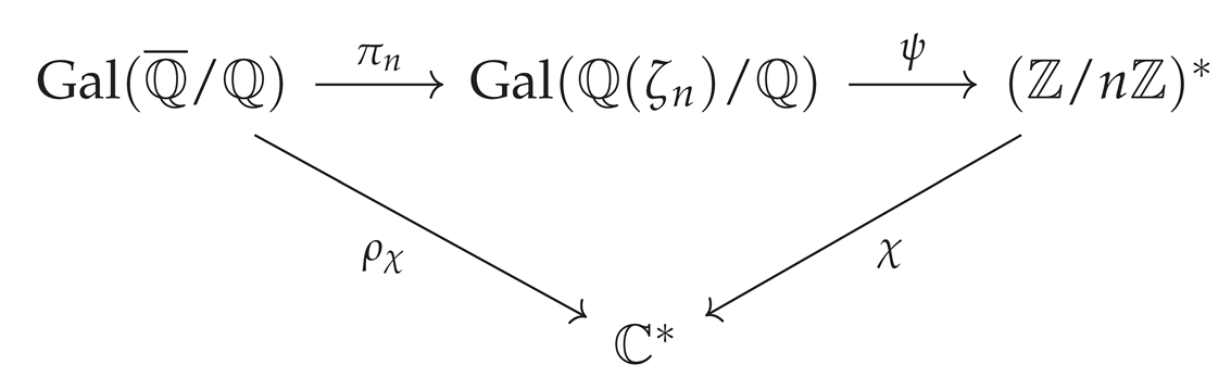${\rho }_{\chi }=\chi \circ \psi \circ {\pi }_n:Gal(\overline{\mathbb{Q}}/\mathbb{Q})\to {\mathbb{C}}^{*}.$

The above statement is reversible, since every continuous homomorphism $Gal(\overline{\mathbb{Q}}/\mathbb{Q})\to {\mathbb{C}}^{*}$ has finite image and therefore factors through the Galois group of some abelian extension $\mathbb{F}/\mathbb{Q}$. The Kronecker–Weber theorem (stated just below) asserts that $\mathbb{F}$ may always be taken to be the n-th cyclotomic field for some n. By taking the minimal such n, we obtain a primitive Dirichlet character. Thus, any one-dimensional continuous complex representation of the absolute Galois group has finite image and arises from a Dirichlet character.

Theorem 7. 

For any continuous homomorphism $\rho :Gal(\overline{\mathbb{Q}}/\mathbb{Q})\to {\mathbb{C}}^{*}$, there exists a Dirichlet character χ, such that $\rho ={\rho }_{\chi }.$

4. Ramification Theory in General

4.1. Foundations of Hilbert’s Ramification Theory

The theory of ramification, developed by David Hilbert in his monumental 1897 report “Zahlbericht,” represents one of the most profound syntheses in algebraic number theory. At its heart lies a simple but revolutionary insight: the behavior of prime numbers in field extensions is not arbitrary but is governed by the symmetries of those extensions. This insight bridges two seemingly disparate worlds: the discrete, arithmetic realm of prime ideals and the continuous, algebraic realm of Galois groups.

4.1.1. The Fundamental Setting

Let K be a number field—a finite extension of $\mathbb{Q}$—and let ${\mathbb{O}}_K$ denote its ring of integers, consisting of all algebraic integers in K. Consider a finite extension L of K, with ring of integers ${\mathbb{O}}_L$. Both ${\mathbb{O}}_K$ and ${\mathbb{O}}_L$ are Dedekind domains, meaning that every nonzero ideal factors uniquely into prime ideals. This unique factorization is the arithmetic analogue of the fundamental theorem of arithmetic and forms the bedrock upon which the theory is built.

Given a nonzero prime ideal $\mathfrak{p}$ in ${\mathbb{O}}_K$, the central question of ramification theory is: How does $\mathfrak{p}$ decompose when extended to ${\mathbb{O}}_L$? In other words, what is the factorization of the ideal $\mathfrak{p}{\mathbb{O}}_L$ in the larger ring? The answer, provided by Dedekind’s theorem, takes the form

$$\mathfrak{p}{\mathbb{O}}_L={\mathfrak{P}}_1^{e_1}{\mathfrak{P}}_2^{e_2}\dots {\mathfrak{P}}_g^{e_g},$$

where the ${\mathfrak{P}}_i$ are distinct prime ideals of ${\mathbb{O}}_L$, and the $e_i$ are positive integers. From this factorization emerge three fundamental invariants that encode the arithmetic behavior of $\mathfrak{p}$ in the extension $L/K$.

4.1.2. The Three Arithmetic Invariants

The ramification index $e_i$ of ${\mathfrak{P}}_i$ over $\mathfrak{p}$ is the exponent with which ${\mathfrak{P}}_i$ appears in the factorization. It measures the multiplicity of the prime ${\mathfrak{P}}_i$ above $\mathfrak{p}$. When $e_i=1$, we say that ${\mathfrak{p}}_i$ is unramified in L; if $e_i>1$, it is ramified. Ramification is a genuinely arithmetic phenomenon—a kind of “branching” that has no direct analogue in the theory of field extensions alone.

The residue field degree $f_i$ is defined as the degree of the extension of residue fields:

$$f_i=[{\mathbb{O}}_L/{\mathfrak{P}}_i:{\mathbb{O}}_K/\mathfrak{p}].$$

Since ${\mathbb{O}}_K/\mathfrak{p}$ and ${\mathbb{O}}_L/{\mathfrak{P}}_i$ are finite fields (the residue fields at $\mathfrak{p}$ and ${\mathfrak{P}}_i$), $f_i$ measures how much the residue field “expands” when we pass from K to L at the prime in question. A simple but instructive way to view $f_i$ is as the dimension of ${\mathbb{O}}_L/{\mathfrak{P}}_i$ as a vector space over ${\mathbb{O}}_K/\mathfrak{p}$.

The third invariant, g, is simply the number of distinct prime ideals ${\mathfrak{P}}_i$ appearing in the factorization. It tells us how many primes in L lie above $\mathfrak{p}$. When $g=1=e$, we say that $\mathfrak{p}$ is inert (it remains prime in L); when $g=[L:K]$, it splits completely.

These three numbers—$e_i$, $f_i$, and g—are not independent. They are bound together by a fundamental relation that reflects the deep interplay between the arithmetic of the extension and its algebraic structure.

4.1.3. The Fundamental Identity

Let $n=[L:K]$ denote the degree of the field extension. Then the invariants satisfy the equation

$$n=\sum _{i=1}^g{e}_i{f}_i.$$

In the special case where $L/K$ is a Galois extension, the Galois group $Gal(L/K)$ acts transitively on the set $\{{\mathfrak{P}}_1,\dots ,{\mathfrak{P}}_g\}$. Consequently, all ramification indices $e_i$ are equal (denote them by e) and all residue field degrees $f_i$ are equal (denote them by f). The fundamental identity then takes the beautifully symmetric form

$$n=e·f·g.$$

This identity is the first great law of ramification theory. It tells us that the degree n, which measures the algebraic complexity of the extension, is partitioned into a product of three arithmetic invariants. In essence, it is a conservation law: the total “amount” of extension (measured by n) is distributed among the three kinds of arithmetic behavior—ramification, residue field extension, and splitting.

To appreciate the identity concretely, consider a quadratic extension $L=\mathbb{Q}\left(\sqrt{d}\right)$ of $\mathbb{Q}$, with d a square-free integer. For an odd prime p not dividing d, the law of quadratic reciprocity determines the decomposition of p:

• If d is a quadratic residue modulo p, then p splits: $e=1$, $f=1$, $g=2$.
• If d is a nonresidue, then p is inert: $e=1$, $f=2$, $g=1$.

If p divides d (and $p\ne 2$), then p ramifies: $e=2$, $f=1$, $g=1$. In every case, $2=e·f·g$.

4.1.4. Two Perspectives on the Proof

The fundamental identity can be proved in several ways, each illuminating a different aspect of the theory. We sketch two particularly instructive approaches.

4.1.4.1 The Arithmetic Approach via Norms

The norm map $N_{L/K}$ sends ideals of ${\mathbb{O}}_L$ to ideals of ${\mathbb{O}}_K$. For a prime ideal $\mathfrak{P}$ of ${\mathbb{O}}_L$ lying above $\mathfrak{p}$, one has

$$N_{L/K}\left(\mathfrak{P}\right)={\mathfrak{p}}^f,$$

where f is the residue field degree of $\mathfrak{P}$ over $\mathfrak{p}$. The norm is multiplicative, so applying it to the factorization $\mathfrak{p}{\mathbb{O}}_L={\prod }_{i=1}^g{\mathfrak{P}}_i^{e_i}$ gives

$$N_{L/K}\left(\mathfrak{p}{\mathbb{O}}_L\right)=\prod _{i=1}^g{N}_{L/K}{\left({\mathfrak{P}}_i\right)}^{e_i}=\prod _{i=1}^g{\left({\mathfrak{p}}^{f_i}\right)}^{e_i}={\mathfrak{p}}^{{\sum }_{i=1}^g{e}_i{f}_i}.$$

On the other hand, for any ideal $\mathfrak{a}$ of ${\mathbb{O}}_K$, one can show that $N_{L/K}\left(\mathfrak{a}{\mathbb{O}}_L\right)={\mathfrak{a}}^{[L:K]}$. Taking $\mathfrak{a}=\mathfrak{p}$ yields $N_{L/K}\left(\mathfrak{p}{\mathbb{O}}_L\right)={\mathfrak{p}}^n$. Comparing the two expressions gives ${\mathfrak{p}}^{\sum e_i{f}_i}={\mathfrak{p}}^n$, whence $\sum e_i{f}_i=n$.

This proof highlights the role of the norm as a bridge between the arithmetic of L and that of K. It is elegant and concise, but it somewhat conceals the local nature of the phenomenon.

4.1.4.2 The Algebraic Approach via Module Lengths

A more structural proof proceeds by localizing at $\mathfrak{p}$. Let $A={\left({\mathbb{O}}_K\right)}_{\mathfrak{p}}$ be the localization of ${\mathbb{O}}_K$ at $\mathfrak{p}$; it is a discrete valuation ring. Similarly, set $B={\left({\mathbb{O}}_L\right)}_{\mathfrak{p}}=S^{-1}{\mathbb{O}}_L$ where $S={\mathbb{O}}_K\setminus \mathfrak{p}$. The ring B is a finitely generated free A-module of rank $n=[L:K]$. The key object is the quotient $B/\mathfrak{p}B$, which is an A-module of finite length.

Since $B\cong A^n$ as A-modules, we have $B/\mathfrak{p}B\cong {(A/\mathfrak{p}A)}^n$ as vector spaces over the residue field $\kappa =A/\mathfrak{p}A$. Hence the length of $B/\mathfrak{p}B$ as an A-module equals n.

On the other hand, by the Chinese remainder theorem,

$$B/\mathfrak{p}B\cong \underset{i=1}{\overset{g}{⨁}}B/{\mathfrak{P}}_i^{e_i},$$

where ${\mathfrak{P}}_i$ now denote the extensions of the original primes to B. The length of each summand $B/{\mathfrak{P}}_i^{e_i}$ can be computed by considering the filtration

$$B/{\mathfrak{P}}_i^{e_i}\supset {\mathfrak{P}}_i/{\mathfrak{P}}_i^{e_i}\supset {\mathfrak{P}}_i^2/{\mathfrak{P}}_i^{e_i}\supset \dots \supset 0.$$

The successive quotients are ${\mathfrak{P}}_i^j/{\mathfrak{P}}_i^{j+1}\cong B/{\mathfrak{P}}_i$, each of which is a one-dimensional vector space over $B/{\mathfrak{P}}_i$ and hence has dimension $f_i$ over $\kappa$. Since there are $e_i$ such quotients, the length of $B/{\mathfrak{P}}_i^{e_i}$ is $e_i{f}_i$. Additivity of length then gives

$$n=\sum _{i=1}^g{e}_i{f}_i.$$

This proof reveals the local nature of ramification: the global identity reduces to a statement about modules over a discrete valuation ring. It also introduces the powerful technique of using module length (a kind of “dimension” for modules over local rings) to measure arithmetic invariants.

4.1.5. Toward a Deeper Theory

The fundamental identity is only the beginning. It tells us that the arithmetic of a prime in an extension is controlled by three numbers, but it does not explain why these numbers take the values they do. The next step, which Hilbert took, is to bring Galois theory into the picture. When $L/K$ is Galois, the Galois group $Gal(L/K)$ acts on the primes above $\mathfrak{p}$, and this action yields a rich structure.

One defines the decomposition group

$$D\left(\mathfrak{P}\right|\mathfrak{p})=\{\sigma \in Gal(L/K):\sigma \left(\mathfrak{P}\right)=\mathfrak{P}\},$$

which measures the symmetry of the prime $\mathfrak{P}$ relative to the extension. Within it lies the inertia group

$$I\left(\mathfrak{P}\right|\mathfrak{p})=\{\sigma \in D\left(\mathfrak{P}\right|\mathfrak{p}):\sigma \left(x\right)\equiv x(mod\mathfrak{P})\mathrm{for}\mathrm{all}x\in {\mathbb{O}}_L\},$$

which captures the “inertial” symmetries that act trivially on the residue field. Remarkably, the orders of these groups are precisely the invariants we have already met:

$$\left|I\right(\mathfrak{P}\left|\mathfrak{p}\right)|=e,|D\left(\mathfrak{P}\right|\mathfrak{p})/I(\mathfrak{P}\left|\mathfrak{p}\right)|=f.$$

Thus, the arithmetic invariants e and f are manifested as the sizes of certain natural subgroups of the Galois group. This connection between group theory and arithmetic is the heart of Hilbert’s ramification theory.

Moreover, when the extension is unramified at $\mathfrak{p}$ (so $e=1$), the inertia group is trivial and the decomposition group is isomorphic to the Galois group of the residue field extension. In this case, there is a canonical generator of $D\left(\mathfrak{P}\right|\mathfrak{p})$, the Frobenius element, which raises elements of the residue field to the q-th power (where q is the size of ${\mathbb{O}}_K/\mathfrak{p}$). The Frobenius element is a central character in modern number theory, linking prime ideals to automorphisms of Galois groups and ultimately to the patterns observed in the distribution of primes.

These ideas—decomposition and inertia groups, the Frobenius element, and the further distinction between tame and wild ramification—form the core of Hilbert’s theory. They will be explored in detail in the next part of this exposition.

4.2. Hilbert’s Main Theorem of Ramification

The fundamental identity $n=e·f·g$ tells us how the degree of an extension is distributed among three arithmetic invariants, but it does not explain why a particular prime $\mathfrak{p}$ behaves the way it does. Why does one prime split completely while another remains inert? Why does ramification occur at certain primes and not others? To answer these questions, we must bring the Galois group into play. Hilbert’s great insight was to realize that the arithmetic of prime decomposition is encoded in the structure of the Galois group through certain natural subgroups. This leads us to the main theorem of ramification theory, which establishes a connection between group theory and arithmetic.

4.2.1. The Galois Action on Primes

Let $L/K$ be a finite Galois extension of number fields with Galois group $G=Gal(L/K)$. The group G acts on the ring ${\mathbb{O}}_L$ and, consequently, on the set of prime ideals of ${\mathbb{O}}_L$. For a prime ideal $\mathfrak{P}$ of ${\mathbb{O}}_L$ and an automorphism $\sigma \in G$, the image $\sigma \left(\mathfrak{P}\right)$ is again a prime ideal of ${\mathbb{O}}_L$. Moreover, if $\mathfrak{P}$ lies above $\mathfrak{p}$ (i.e., $\mathfrak{P}\cap {\mathbb{O}}_K=\mathfrak{p}$), then $\sigma \left(\mathfrak{P}\right)$ also lies above $\mathfrak{p}$ because $\sigma$ fixes K pointwise. This action is transitive: given any two primes $\mathfrak{P}$ and ${\mathfrak{P}}^{\prime }$ above $\mathfrak{p}$, there exists $\sigma \in G$ such that $\sigma \left(\mathfrak{P}\right)={\mathfrak{P}}^{\prime }$. This transitivity is a key reason why, in a Galois extension, all ramification indices $e_i$ and residue field degrees $f_i$ are equal (we denote them simply by e and f).

The stabilizer of a prime $\mathfrak{P}$ under this action is called the decomposition group:

$$D_{\mathfrak{P}}=\{\sigma \in G:\sigma \left(\mathfrak{P}\right)=\mathfrak{P}\}.$$

The decomposition group measures the symmetries of $\mathfrak{P}$ relative to the extension. Its importance stems from the fact that it “controls” the splitting behavior of $\mathfrak{p}$ in L. Indeed, the orbit-stabilizer theorem tells us that the number of primes above $\mathfrak{p}$ is exactly the index of $D_{\mathfrak{P}}$ in G; that is,

$$g=[G:D_{\mathfrak{P}}].$$

But the decomposition group does more than just count primes. Since every $\sigma \in D_{\mathfrak{P}}$ fixes $\mathfrak{P}$ as a set, it induces an automorphism of the residue field ${\mathbb{O}}_L/\mathfrak{P}$. Moreover, because $\sigma$ fixes K, this induced automorphism fixes the subfield ${\mathbb{O}}_K/\mathfrak{p}$. Thus we obtain a homomorphism

$$\phi :D_{\mathfrak{P}}\to Gal(({\mathbb{O}}_L/\mathfrak{P})/({\mathbb{O}}_K/\mathfrak{p})).$$

The kernel of this homomorphism is the inertia group:

$$I_{\mathfrak{P}}=\{\sigma \in D_{\mathfrak{P}}:\sigma \left(x\right)\equiv x(mod\mathfrak{P})\mathrm{for}\mathrm{all}x\in {\mathbb{O}}_L\}.$$

In other words, $I_{\mathfrak{P}}$ consists of those automorphisms that act trivially on the residue field. The inertia group captures the “inertial” part of the decomposition group—those symmetries that are invisible at the level of residue fields.

4.2.2. Hilbert’s Main Theorem

The groups $D_{\mathfrak{P}}$ and $I_{\mathfrak{P}}$ are not arbitrary subgroups of G; their sizes are precisely the arithmetic invariants we introduced earlier. This is the content of Hilbert’s main theorem on ramification.

Theorem 8 

(Hilbert). Let $L/K$ be a finite Galois extension of number fields with Galois group $G=Gal(L/K)$, and let $\mathfrak{P}$ be a prime ideal of ${\mathbb{O}}_L$ lying above a prime $\mathfrak{p}$ of ${\mathbb{O}}_K$. Then:

1.

The decomposition group $D_{\mathfrak{P}}$ has order $e·f$, where e is the ramification index and f is the residue field degree of $\mathfrak{P}$ over $\mathfrak{p}$.

2.

The inertia group $I_{\mathfrak{P}}$ has order e.

3.

The quotient $D_{\mathfrak{P}}/I_{\mathfrak{P}}$ is isomorphic to the Galois group of the residue field extension:

$$D_{\mathfrak{P}}/I_{\mathfrak{P}}\cong Gal(({\mathbb{O}}_L/\mathfrak{P})/({\mathbb{O}}_K/\mathfrak{p})).$$

In particular, $|D_{\mathfrak{P}}/I_{\mathfrak{P}}|=f$.

4.2.3. Detailed Proof of Hilbert’s Theorem

We now provide a complete proof of Hilbert’s theorem. The proof will proceed in several steps, combining group theory, commutative algebra, and the arithmetic of local fields.

4.2.3.1 Step 1: Transitivity and the order of $D_{\mathfrak{P}}$

Since G acts transitively on the set of primes above $\mathfrak{p}$, the orbit of $\mathfrak{P}$ has size g. By the orbit-stabilizer theorem, we have

$$\left|G\right|=g·|D_{\mathfrak{P}}|.$$

But $\left|G\right|=[L:K]=n$, and by the fundamental identity $n=e·f·g$. Therefore,

$$|D_{\mathfrak{P}}|={\displaystyle \frac{\left|G\right|}{g}}={\displaystyle \frac{e·f·g}{g}}=e·f.$$

This establishes the first part of the theorem.

4.2.3.2 Step 2: The inertia group and the surjectivity map

Consider the reduction modulo $\mathfrak{P}$ map

$$\pi :{\mathbb{O}}_L\to {\mathbb{O}}_L/\mathfrak{P}.$$

For $\sigma \in D_{\mathfrak{P}}$, the condition $\sigma \left(\mathfrak{P}\right)=\mathfrak{P}$ ensures that $\sigma$ induces an automorphism $\overline{\sigma }$ of ${\mathbb{O}}_L/\mathfrak{P}$ that fixes ${\mathbb{O}}_K/\mathfrak{p}$ elementwise. This gives a homomorphism

$$\phi :D_{\mathfrak{P}}\to Gal(({\mathbb{O}}_L/\mathfrak{P})/({\mathbb{O}}_K/\mathfrak{p})),\sigma \mapsto \overline{\sigma }.$$

The kernel of $\phi$ is precisely $I_{\mathfrak{P}}$, by definition. Thus we have an injective homomorphism

$$D_{\mathfrak{P}}/I_{\mathfrak{P}}\hookrightarrow Gal(({\mathbb{O}}_L/\mathfrak{P})/({\mathbb{O}}_K/\mathfrak{p})).$$

In particular,

$$|D_{\mathfrak{P}}/I_{\mathfrak{P}}|\le f.$$

To prove equality, we need to show that $\phi$ is surjective. This is the most subtle part of the proof. We will use a lifting argument based on Hensel’s lemma. First, note that the extension ${\mathbb{O}}_L/\mathfrak{P}$ over ${\mathbb{O}}_K/\mathfrak{p}$ is separable (since finite fields are perfect).

Now we follow Neukirch’s proof by reduction to the local case. Consider the completions $K_{\mathfrak{p}}$ and $L_{\mathfrak{P}}$ with respect to the $\mathfrak{p}$-adic and $\mathfrak{P}$-adic topologies. We have:

• $L_{\mathfrak{P}}/K_{\mathfrak{p}}$ is a finite Galois extension.
• There is a natural isomorphism $Gal(L_{\mathfrak{P}}/K_{\mathfrak{p}})\cong D_{\mathfrak{P}}$.
• The residue fields are unchanged: $\kappa \left(\mathfrak{P}{\mathbb{O}}_{L_{\mathfrak{P}}}\right)\cong \kappa \left(\mathfrak{P}\right)$ and $\kappa \left(\mathfrak{p}{\mathbb{O}}_{K_{\mathfrak{p}}}\right)\cong \kappa \left(\mathfrak{p}\right)$.
• The inertia group for the local extension corresponds to $I_{\mathfrak{P}}$ under this isomorphism.

Let us denote for simplicity:

$$\widehat{K}=K_{\mathfrak{p}},\widehat{L}=L_{\mathfrak{P}},\widehat{\mathfrak{p}}=\mathfrak{p}{\widehat{\mathbb{O}}}_K,\widehat{\mathfrak{P}}=\mathfrak{P}{\widehat{\mathbb{O}}}_L.$$

Then $\widehat{L}/\widehat{K}$ is a Galois extension of complete discrete valuation fields with Galois group $D_{\mathfrak{P}}$, and $\widehat{\mathfrak{P}}$ is the unique prime above $\widehat{\mathfrak{p}}$.

We now prove that the homomorphism

$$\widehat{\phi }:D_{\mathfrak{P}}\to Gal(\kappa \left(\widehat{\mathfrak{P}}\right)/\kappa \left(\widehat{\mathfrak{p}}\right))\cong Gal(\kappa \left(\mathfrak{P}\right)/\kappa \left(\mathfrak{p}\right))$$

is surjective. Let $\overline{\tau }\in Gal(\kappa \left(\mathfrak{P}\right)/\kappa \left(\mathfrak{p}\right))$.

Choose a primitive element $\overline{\alpha }\in \kappa \left(\mathfrak{P}\right)$ of the extension $\kappa \left(\mathfrak{P}\right)/\kappa \left(\mathfrak{p}\right)$. Let $\alpha \in {\widehat{\mathbb{O}}}_L$ be a lift of $\overline{\alpha }$ (note: we are now in the complete local ring). Let $f\left(x\right)\in {\widehat{\mathbb{O}}}_K\left[x\right]$ be the minimal polynomial of $\alpha$ over $\widehat{K}$. Since $\widehat{L}/\widehat{K}$ is Galois, $f\left(x\right)$ splits completely in $\widehat{L}$.

Let $\overline{f}\left(x\right)\in \kappa \left(\mathfrak{p}\right)\left[x\right]$ be the reduction of $f\left(x\right)$ modulo $\widehat{\mathfrak{p}}$. Then $\overline{\alpha }$ is a root of $\overline{f}\left(x\right)$. Let $\overline{m}\left(x\right)\in \kappa \left(\mathfrak{p}\right)\left[x\right]$ be the minimal polynomial of $\overline{\alpha }$ over $\kappa \left(\mathfrak{p}\right)$. Since $\kappa \left(\mathfrak{p}\right)$ is a finite field (hence perfect), $\overline{\alpha }$ is a simple root of $\overline{m}\left(x\right)$. Moreover, $\overline{m}\left(x\right)$ divides $\overline{f}\left(x\right)$.

Now $\overline{\tau }\left(\overline{\alpha }\right)$ is another root of $\overline{m}\left(x\right)$, hence also a root of $\overline{f}\left(x\right)$. By Hensel’s lemma (applicable because $\widehat{K}$ is complete and $\overline{\alpha }$ is a simple root of $\overline{m}\left(x\right)$), there exists a unique root $\beta \in {\widehat{\mathbb{O}}}_L$ of $f\left(x\right)$ such that $\overline{\beta }=\overline{\tau }\left(\overline{\alpha }\right)$.

Since $f\left(x\right)$ is irreducible over $\widehat{K}$ and $\widehat{L}$ is its splitting field, there exists $\sigma \in Gal(\widehat{L}/\widehat{K})=D_{\mathfrak{P}}$ such that $\sigma \left(\alpha \right)=\beta$.

We claim that $\sigma$ induces $\overline{\tau }$ on the residue field. For any $\overline{x}\in \kappa \left(\mathfrak{P}\right)$, write $\overline{x}=h\left(\overline{\alpha }\right)$ with $h\left(x\right)\in \kappa \left(\mathfrak{p}\right)\left[x\right]$. Lift h to $H\left(x\right)\in {\widehat{\mathbb{O}}}_K\left[x\right]$. Then $x=H\left(\alpha \right)+y$ for some $y\in \widehat{\mathfrak{P}}$. We have:

$$\sigma \left(x\right)=H\left(\beta \right)+\sigma \left(y\right).$$

Reducing modulo $\widehat{\mathfrak{P}}$, and noting that $\sigma \left(y\right)\in \widehat{\mathfrak{P}}$ because $\sigma$ preserves the valuation ring, we obtain:

$$\overline{\sigma \left(x\right)}=\overline{H}\left(\overline{\beta }\right)=\overline{H}\left(\overline{\tau }\left(\overline{\alpha }\right)\right)=\overline{\tau }\left(\overline{H}\left(\overline{\alpha }\right)\right)=\overline{\tau }\left(\overline{x}\right).$$

Thus $\widehat{\phi }\left(\sigma \right)=\overline{\tau }$, proving that $\widehat{\phi }$ is surjective.

Since $\widehat{\phi }$ is exactly the same as $\phi$ under the identification of residue fields, we conclude that $\phi$ is surjective. Therefore

$$D_{\mathfrak{P}}/I_{\mathfrak{P}}\cong Gal(({\mathbb{O}}_L/\mathfrak{P})/({\mathbb{O}}_K/\mathfrak{p})).$$

Consequently, $|D_{\mathfrak{P}}/I_{\mathfrak{P}}|=f$.

4.2.3.3 Step 3: The order of the inertia group

From Step 1 we have $|D_{\mathfrak{P}}|=e·f$, and from Step 2 we have $|D_{\mathfrak{P}}/I_{\mathfrak{P}}|=f$. Therefore,

$$|I_{\mathfrak{P}}|={\displaystyle \frac{|D_{\mathfrak{P}}|}{|D_{\mathfrak{P}}/I_{\mathfrak{P}}|}}={\displaystyle \frac{e·f}{f}}=e.$$

This completes the proof of the theorem.

4.2.4. Interpretations and Consequences

Hilbert’s theorem provides a group-theoretic interpretation of ramification and splitting. The inertia group $I_{\mathfrak{P}}$ measures the extent of ramification: if $I_{\mathfrak{P}}$ is trivial, then $e=1$ and $\mathfrak{p}$ is unramified in L; if $I_{\mathfrak{P}}$ is nontrivial, then $e>1$ and we have ramification. Moreover, the size of $I_{\mathfrak{P}}$ tells us exactly how much ramification occurs.

The quotient $D_{\mathfrak{P}}/I_{\mathfrak{P}}$ is isomorphic to the Galois group of a finite extension of finite fields. Such extensions are always cyclic, generated by the Frobenius automorphism $x\mapsto x^{|{\mathbb{O}}_K/\mathfrak{p}|}$. Therefore, when $\mathfrak{P}$ is unramified (so $I_{\mathfrak{P}}=1$), we have $D_{\mathfrak{P}}\cong Gal(({\mathbb{O}}_L/\mathfrak{P})/({\mathbb{O}}_K/\mathfrak{p}))$, and this group is cyclic. In this case, the preimage in $D_{\mathfrak{P}}$ of the Frobenius automorphism is called the Frobenius element at $\mathfrak{P}$, denoted ${Frob}_{\mathfrak{P}}$. It is a crucial actor in number theory, linking prime ideals to elements of the Galois group. The Frobenius element satisfies

$${Frob}_{\mathfrak{P}}\left(x\right)\equiv x^{|{\mathbb{O}}_K/\mathfrak{p}|}(mod\mathfrak{P})\mathrm{for}\mathrm{all}x\in {\mathbb{O}}_L.$$

When $L/K$ is abelian (i.e., the Galois group is abelian), the Frobenius element depends only on $\mathfrak{p}$, not on the choice of $\mathfrak{P}$ above $\mathfrak{p}$, and is denoted ${Frob}_{\mathfrak{p}}$. This is the starting point for class field theory and modern reciprocity laws.

Another important consequence of Hilbert’s theorem is the understanding of how primes decompose in intermediate fields. If $K\subseteq E\subseteq L$ is an intermediate field, and ${\mathfrak{P}}_E=\mathfrak{P}\cap {\mathbb{O}}_E$, then the decomposition and inertia groups of $\mathfrak{P}$ over E are simply the subgroups of $D_{\mathfrak{P}}$ and $I_{\mathfrak{P}}$ corresponding to the extension $L/E$ under the Galois correspondence. This allows us to relate the splitting of $\mathfrak{p}$ in E to the splitting of ${\mathfrak{P}}_E$ in L, providing a powerful tool for studying the decomposition of primes in towers of fields.

4.2.5. An Example: Decomposition and inertia groups in a quadratic extension

Let $L/\mathbb{Q}$ be a quadratic extension. Then $L/\mathbb{Q}$ is Galois with Galois group

$$G=Gal(L/\mathbb{Q})=\{\mathrm{id},\sigma \}.$$

Let p be an odd prime, and let $\mathfrak{P}$ be a prime ideal of ${\mathbb{O}}_L$ lying above p. We distinguish cases according to the factorization of $p{\mathbb{O}}_L$.

• Split case. If $p{\mathbb{O}}_L={\mathfrak{P}}_1{\mathfrak{P}}_2,\mathrm{with}{\mathfrak{P}}_1\ne {\mathfrak{P}}_2,$ then the nontrivial automorphism $\sigma$ exchanges ${\mathfrak{P}}_1$ and ${\mathfrak{P}}_2$. Hence the only element of G fixing ${\mathfrak{P}}_1$ is the identity, and therefore $D_{{\mathfrak{P}}_1}=\left\{\mathrm{id}\right\}.$ Thus $|D_{{\mathfrak{P}}_1}|=1$, and indeed $e=1$ and $f=1$. Since $e=1$, the inertia group is trivial: $I_{{\mathfrak{P}}_1}=\left\{\mathrm{id}\right\}.$
• Inert case. If $p{\mathbb{O}}_L=\mathfrak{P}$ is prime, then $\mathfrak{P}$ is the unique prime ideal above p. Consequently every automorphism in G fixes $\mathfrak{P}$, and hence $D_{\mathfrak{P}}=G.$ In this case $e=1$ and $f=2$, so $|D_{\mathfrak{P}}|=ef=2$. Since $e=1$, the inertia group is again trivial: $I_{\mathfrak{P}}=\left\{\mathrm{id}\right\}.$
• Ramified case. If p ramifies in L, equivalently if $p\mid disc\left(L\right)$, then $p{\mathbb{O}}_L={\mathfrak{P}}^2.$ As $\mathfrak{P}$ is the unique prime ideal above p, we again have $D_{\mathfrak{P}}=G.$ Here the ramification index is $e=2$ and the residue degree is $f=1$, so the inertia group has order 2. Since $\left|G\right|=2$, it follows that $I_{\mathfrak{P}}=G.$ Equivalently, the nontrivial automorphism $\sigma$ acts trivially on the residue field ${\mathbb{O}}_L/\mathfrak{P}$.

In summary, in both the inert and ramified cases the decomposition group coincides with the full Galois group G, while the inertia group distinguishes the two phenomena: it is trivial in the inert case and equal to G in the ramified case.

4.2.6. Cyclotomic Extensions: A Paradigmatic Example

Cyclotomic extensions provide perhaps the most important class of examples in algebraic number theory where Hilbert’s theory can be applied with full precision and yields remarkably complete results. Let m be a positive integer, and consider the cyclotomic field $L=\mathbb{Q}\left({\zeta }_m\right)$, where ${\zeta }_m$ is a primitive mth root of unity. The extension $L/\mathbb{Q}$ is Galois, and its Galois group is canonically isomorphic to ${(\mathbb{Z}/m\mathbb{Z})}^{\times }$, with an element $a\in {(\mathbb{Z}/m\mathbb{Z})}^{\times }$ corresponding to the automorphism ${\sigma }_a$ defined by ${\sigma }_a\left({\zeta }_m\right)={\zeta }_m^a$.

Let p be a rational prime. The decomposition of p in L depends crucially on the relationship between p and m. We distinguish two cases.

Case 1: $p\nmid m$. In this case p is unramified in L. The residue field degree f is the order of p modulo m, i.e., the smallest positive integer f such that $p^f\equiv 1(modm)$. The number of primes above p is $g=\phi \left(m\right)/f$, where $\phi$ is Euler’s totient function, and $e=1$. The decomposition group $D_{\mathfrak{P}}$ for a prime $\mathfrak{P}$ above p is cyclic of order f, generated by the Frobenius element ${Frob}_{\mathfrak{P}}$, which corresponds to $p\in {(\mathbb{Z}/m\mathbb{Z})}^{\times }$ under the isomorphism $Gal(L/\mathbb{Q})\cong {(\mathbb{Z}/m\mathbb{Z})}^{\times }$. More precisely, ${Frob}_{\mathfrak{P}}$ is the automorphism ${\sigma }_p:{\zeta }_m\mapsto {\zeta }_m^p$. This follows from the fact that modulo $\mathfrak{P}$, we have ${Frob}_{\mathfrak{P}}\left({\zeta }_m\right)\equiv {\zeta }_m^p(mod\mathfrak{P})$, and since both sides are mth roots of unity and $p\nmid m$, the congruence is actually an equality. The inertia group $I_{\mathfrak{P}}$ is trivial.

Case 2: $p\mid m$. Write $m=p^k{m}^{\prime }$ with $p\nmid m^{\prime }$. In this case, p is ramified in L. Specifically, the ramification index in the extension $\mathbb{Q}\left({\zeta }_m\right)/\mathbb{Q}$ is $e=\phi \left(p^k\right)=p^{k-1}(p-1)$, while the residue field degree f is the order of p modulo $m^{\prime }$ (i.e., the smallest positive integer f such that $p^f\equiv 1(mod{m}^{\prime })$). The number of primes above p is $g=\phi \left(m^{\prime }\right)/f$.

To understand the decomposition and inertia groups, consider the tower of fields:

$$\mathbb{Q}\subseteq \mathbb{Q}\left({\zeta }_{m^{\prime }}\right)\subseteq \mathbb{Q}\left({\zeta }_m\right)=L.$$

The extension $\mathbb{Q}\left({\zeta }_{m^{\prime }}\right)/\mathbb{Q}$ is unramified at p, while the extension $\mathbb{Q}\left({\zeta }_m\right)/\mathbb{Q}\left({\zeta }_{m^{\prime }}\right)$ is totally ramified at every prime lying above p. Consequently, for a prime $\mathfrak{P}$ of L lying above p, we have:

• The inertia group $I_{\mathfrak{P}}$ is isomorphic to $Gal(\mathbb{Q}\left({\zeta }_m\right)/\mathbb{Q}\left({\zeta }_{m^{\prime }}\right))\cong {(\mathbb{Z}/p^k\mathbb{Z})}^{\times }$, and has order $e=\phi \left(p^k\right)$.
• The decomposition group $D_{\mathfrak{P}}$ consists of those automorphisms ${\sigma }_a\in Gal(L/\mathbb{Q})$ for which $amod{m}^{\prime }$ is a power of p modulo $m^{\prime }$. More precisely, under the isomorphism $Gal(L/\mathbb{Q})\cong {(\mathbb{Z}/m\mathbb{Z})}^{\times }$, the decomposition group corresponds to the subgroup

  $$\{a\in {(\mathbb{Z}/m\mathbb{Z})}^{\times }\mid a\equiv p^j(mod{m}^{\prime })\mathrm{for}\mathrm{some}j\}.$$
  Under the natural isomorphism ${(\mathbb{Z}/m\mathbb{Z})}^{\times }\cong {(\mathbb{Z}/p^k\mathbb{Z})}^{\times }\times {(\mathbb{Z}/m^{\prime }\mathbb{Z})}^{\times }$, this subgroup corresponds to ${(\mathbb{Z}/p^k\mathbb{Z})}^{\times }\times \langle p\rangle$, where $\langle p\rangle$ denotes the cyclic subgroup generated by p in ${(\mathbb{Z}/m^{\prime }\mathbb{Z})}^{\times }$. Its order is $e·f$.
• The quotient $D_{\mathfrak{P}}/I_{\mathfrak{P}}$ is cyclic of order f, and is isomorphic to $Gal\left(\kappa \right(\mathfrak{P})/\kappa (p\left)\right)$, where $\kappa \left(\mathfrak{P}\right)$is the residue field of $\mathfrak{P}$.

To see why p is totally ramified in $\mathbb{Q}\left({\zeta }_{p^k}\right)$, consider the minimal polynomial of ${\zeta }_{p^k}$ over $\mathbb{Q}$, which is the $p^k$th cyclotomic polynomial ${\Phi }_{p^k}\left(x\right)=x^{p^{k-1}(p-1)}+\dots +x^{p^{k-1}}+1$. Modulo p, we have ${\Phi }_{p^k}\left(x\right)\equiv {(x-1)}^{\phi \left(p^k\right)}(modp)$, so the only prime above p is $\mathfrak{P}=(p,{\zeta }_{p^k}-1)$, and $p{\mathbb{O}}_L={\mathfrak{P}}^{\phi \left(p^k\right)}$.

These results illustrate the power of Hilbert’s theorem: the abstract group-theoretic definitions of decomposition and inertia groups match perfectly with explicit computations in cyclotomic fields. Moreover, the Frobenius element emerges naturally as the automorphism raising roots of unity to the pth power, providing a clear arithmetic interpretation of the Galois action.

4.2.7. Wild and Tame Ramification

Hilbert’s theorem tells us that the inertia group has order e, but it does not reveal the full structure of this group. In fact, the inertia group can be further decomposed. When the ramification index e is coprime to the characteristic of the residue field, we say the ramification is tame. In this case, the inertia group is cyclic of order e. However, when e is divisible by the residue characteristic, the ramification is wild, and the inertia group is more complicated—it is a semidirect product of a cyclic group of order prime to the characteristic and a p-group. The study of wild ramification leads to higher ramification groups, which provide a filtration of the inertia group by deeper and deeper “layers” of ramification. This finer structure is essential for understanding the behavior of primes in extensions of fields of positive characteristic, and it also appears in the study of local fields in characteristic zero.

4.2.8. Conclusion

Hilbert’s main theorem of ramification transforms the arithmetic of prime decomposition into a problem in group theory. By associating to each prime $\mathfrak{P}$ the decomposition and inertia groups, we obtain a powerful language for describing how primes split, remain inert, or ramify in a Galois extension. This language is not merely descriptive; it is predictive, allowing us to deduce splitting patterns from the structure of the Galois group and vice versa.

The theorem also lays the foundation for class field theory, where the Frobenius element becomes a key player in the Artin reciprocity law. Moreover, the distinction between tame and wild ramification leads to a rich theory of higher ramification groups, developed by Hilbert and later refined by Hasse, Herbrand.

In the next part, we will explore the Frobenius element in detail and discuss its role in the Chebotarev density theorem, which describes the statistical distribution of splitting types among primes in a Galois extension.

4.3. The Frobenius Element and the Chebotarev Density Theorem

4.3.1. The Arithmetic of Frobenius

The Frobenius element stands as one of the most important concepts in algebraic number theory. Born from Hilbert’s ramification theory, it serves as the critical bridge between the discrete arithmetic of prime ideals and the continuous symmetries of Galois groups. In its essence, the Frobenius element encodes the action of a prime ideal on the Galois group of an extension, transforming the study of prime decomposition into a problem of equidistribution in finite groups.

The Chebotarev density theorem, proved by Nikolai Chebotarev in 1925, generalizes both Dirichlet’s theorem on primes in arithmetic progressions and the prime number theorem for number fields. It states that the Frobenius elements are equidistributed in the Galois group according to the Haar measure. This result not only provides a beautiful and complete description of how primes split in Galois extensions but also lays the foundation for modern reciprocity laws and the Langlands program.

In this part, we shall develop the theory of the Frobenius element with full rigor, prove the Chebotarev density theorem, and explore its far-reaching consequences. We assume familiarity with Hilbert’s main theorem of ramification (8) and the basic theory of Dedekind zeta functions.

4.3.2. The Frobenius Element: Definition and Basic Properties

Let $L/K$ be a finite Galois extension of number fields with Galois group $G=Gal(L/K)$. Let $\mathfrak{P}$ be a prime ideal of ${\mathbb{O}}_L$ lying above a prime $\mathfrak{p}$ of ${\mathbb{O}}_K$. Assume that $\mathfrak{p}$ is unramified in L, i.e., the ramification index $e\left(\mathfrak{P}\right|\mathfrak{p})=1$. Then by Hilbert’s theorem, the decomposition group $D_{\mathfrak{P}}$ is isomorphic to the Galois group of the residue field extension:

$$D_{\mathfrak{P}}\cong Gal(({\mathbb{O}}_L/\mathfrak{P})/({\mathbb{O}}_K/\mathfrak{p})).$$

Since the residue field extension is finite and separable (indeed, finite fields are perfect), it is cyclic. Let $q=|{\mathbb{O}}_K/\mathfrak{p}|$ be the cardinality of the residue field. The Galois group of a finite extension of finite fields is generated by the Frobenius automorphism${\phi }_q:x\mapsto x^q$.

Definition 6 

(Frobenius element). TheFrobenius element${Frob}_{\mathfrak{P}}\in D_{\mathfrak{P}}\subseteq G$ is the unique automorphism corresponding to ${\phi }_q$ under the isomorphism $D_{\mathfrak{P}}\cong Gal(({\mathbb{O}}_L/\mathfrak{P})/({\mathbb{O}}_K/\mathfrak{p}))$. Equivalently, ${Frob}_{\mathfrak{P}}$ is the unique element of G satisfying

$${Frob}_{\mathfrak{P}}\left(x\right)\equiv x^q(mod\mathfrak{P})\mathrm{for}\mathrm{all}x\in {\mathbb{O}}_L.$$

The Frobenius element is a central concept because it attaches to each unramified prime $\mathfrak{p}$ (and a choice of prime $\mathfrak{P}$ above it) an element of the Galois group. When the extension $L/K$ is abelian, i.e., G is abelian, the Frobenius element depends only on $\mathfrak{p}$, not on the choice of $\mathfrak{P}$. In this case, we denote it by ${Frob}_{\mathfrak{p}}$.

Proposition 1 

(Properties of the Frobenius element). Let $\mathfrak{P}$ be a prime above an unramified prime $\mathfrak{p}$.

1.

The Frobenius element ${Frob}_{\mathfrak{P}}$ has order equal to the residue field degree $f\left(\mathfrak{P}\right|\mathfrak{p})$.

2.

For any $\sigma \in G$, we have ${Frob}_{\sigma \left(\mathfrak{P}\right)}=\sigma {Frob}_{\mathfrak{P}}{\sigma }^{-1}$. Hence the conjugacy class of ${Frob}_{\mathfrak{P}}$ depends only on $\mathfrak{p}$.

3.

If E is an intermediate field corresponding to a subgroup $H\subseteq G$ under the Galois correspondence, then the Frobenius element for $\mathfrak{P}\cap {\mathbb{O}}_E$ in $Gal(E/K)$ is the image of ${Frob}_{\mathfrak{P}}$ under the restriction map $G\to Gal(E/K)$.

Proof. (1) Since ${Frob}_{\mathfrak{P}}$ corresponds to the generator of a cyclic group of order f, its order is f. (2) For any $x\in {\mathbb{O}}_L$, we have

$$\sigma {Frob}_{\mathfrak{P}}{\sigma }^{-1}\left(x\right)\equiv \sigma \left({\left({\sigma }^{-1}\left(x\right)\right)}^q\right)\equiv \sigma \left({\sigma }^{-1}\left(x^q\right)\right)\equiv x^q(mod\sigma \left(\mathfrak{P}\right)),$$

so $\sigma {Frob}_{\mathfrak{P}}{\sigma }^{-1}$ satisfies the defining property of ${Frob}_{\sigma \left(\mathfrak{P}\right)}$. (3) This follows from the compatibility of the residue field extensions. □

Thus, to each unramified prime $\mathfrak{p}$, we associate a conjugacy class $C_{\mathfrak{p}}\subseteq G$ consisting of all ${Frob}_{\mathfrak{P}}$ for primes $\mathfrak{P}$ above $\mathfrak{p}$. This conjugacy class is the fundamental invariant of $\mathfrak{p}$ in the Galois extension.

4.3.3. The Chebotarev Density Theorem: Statement and Significance

Let $L/K$ be a finite Galois extension of number fields with Galois group $G=Gal(L/K)$. For a prime ideal $\mathfrak{p}$ of K that is unramified in L, choose a prime ideal $\mathfrak{P}$ of L lying above $\mathfrak{p}$. The Frobenius element ${Frob}_{\mathfrak{P}}\in G$ is well-defined up to conjugation; its conjugacy class depends only on $\mathfrak{p}$, not on the choice of $\mathfrak{P}$. We denote this conjugacy class by $C_{\mathfrak{p}}$.

For a conjugacy class $C\subseteq G$, define

$${\pi }_C\left(x\right)=\#\{\mathfrak{p}\mathrm{prime}\mathrm{of}K:\mathfrak{p}\mathrm{unramified}\mathrm{in}L,N\mathfrak{p}\le x,C_{\mathfrak{p}}=C\},$$

where $N\mathfrak{p}=|{\mathbb{O}}_K/\mathfrak{p}|$ is the absolute norm. Let

$${\pi }_K\left(x\right)=\#\{\mathfrak{p}\mathrm{prime}\mathrm{of}K:N\mathfrak{p}\le x\}$$

be the number of all prime ideals of K (ramified or unramified) with norm at most x.

Theorem 9 

(Chebotarev Density Theorem). With the notation above, the natural density of the set of unramified primes $\mathfrak{p}$ of K with Frobenius conjugacy class C exists and equals $\left|C\right|/\left|G\right|$. That is,

$$\underset{x\to \infty }{lim}{\displaystyle \frac{{\pi }_C\left(x\right)}{{\pi }_K\left(x\right)}}={\displaystyle \frac{\left|C\right|}{\left|G\right|}}.$$

Equivalently, the Dirichlet density of this set is also $\left|C\right|/\left|G\right|$.

The theorem asserts that the Frobenius elements are equidistributed among the conjugacy classes of G as $\mathfrak{p}$ varies over the unramified primes of K. In particular, for every conjugacy class C, there are infinitely many primes $\mathfrak{p}$ with $C_{\mathfrak{p}}=C$, and the frequency with which they occur is proportional to the size of C. Every conjugacy class occurs as the Frobenius class for infinitely many primes. This result generalizes Dirichlet’s theorem (which corresponds to the case $K=\mathbb{Q}$, $L=\mathbb{Q}\left({\zeta }_m\right)$) and the prime number theorem for number fields.

4.3.4. Sketch of the Proof via Artin L-Functions

The proof requires several deep results from class field theory and analytic number theory.

4.3.4.1 Step 1: Reduction to cyclic extensions

We first reduce the problem to the case where G is cyclic. Let $L/K$ be a finite Galois extension of number fields with Galois group $G=Gal(L/K)$. The analytic input required for the proof of Chebotarev’s density theorem is the following statement:

For every non-trivial irreducible character χ of G, the Artin L-function $L(s,\chi ,L/K)$ is holomorphic for $\Re \left(s\right)>1$, admits a meromorphic continuation to $\Re \left(s\right)\ge 1$, and has no zeros on the line $\Re \left(s\right)=1$.

Once this statement is known, Chebotarev’s density theorem follows from a standard Tauberian argument. We now explain how this analytic assertion reduces to the case of cyclic extensions.

• Brauer induction. By Brauer’s induction theorem, every irreducible character $\chi$ of G can be written as a finite $\mathbb{Z}$-linear combination

  $$\chi =\sum _{i=1}^r{n}_i{Ind}_{H_i}^G\left({\psi }_i\right),n_i\in \mathbb{Z},$$

  where each $H_i\subseteq G$ is an elementary subgroup and ${\psi }_i$ is a linear character of $H_i$. Recall that an elementary subgroup is a direct product of a p-group and a cyclic group of order prime to p.
• Artin formalism. Artin’s formalism for L-functions yields the factorization

  $$L(s,\chi ,L/K)=\prod _{i=1}^{r}L{(s,{\psi }_i,L/L^{H_i})}^{n_i},$$

  where $L(s,{\psi }_i,L/L^{H_i})$ denotes the Artin L-function associated with the linear character ${\psi }_i$ of

  $$H_i=Gal(L/L^{H_i}).$$
• Passage to cyclic extensions. Since ${\psi }_i$ is linear, its kernel $\mathsf{Ker}{\psi }_i$ has finite index in $H_i$, and the quotient $H_i/\mathsf{Ker}{\psi }_i$ is a finite cyclic group. Let

  $$M_i=L^{\mathsf{Ker}{\psi }_i}.$$
  Then $M_i/L^{H_i}$ is a finite cyclic extension. By Artin reciprocity, the Artin L-function $L(s,{\psi }_i,L/L^{H_i})$ coincides with the Hecke L-function attached to the corresponding Hecke character of the cyclic extension $M_i/L^{H_i}$.
• Analytic reduction. Assume the following analytic statement:
  For every finite cyclic extension $M/F$ of number fields and every non-trivial Hecke character φ associated with $M/F$, the Hecke L-function $L(s,\phi )$ is holomorphic for $\Re \left(s\right)>1$, admits a meromorphic continuation to $\Re \left(s\right)\ge 1$, and has no zeros on the line $\Re \left(s\right)=1$.
  Under this assumption, each factor $L(s,{\psi }_i,L/L^{H_i})$ with ${\psi }_i$ non-trivial satisfies the required analytic properties. The factors corresponding to trivial linear characters give rise to Dedekind zeta functions of intermediate fields; in the Brauer decomposition of a non-trivial irreducible character $\chi$, their contributions cancel in such a way that no pole at $s=1$ occurs. Consequently, the Artin L-function $L(s,\chi ,L/K)$ satisfies the analytic statement above for every non-trivial irreducible character $\chi$ of G.
• Conclusion. Thus the analytic part of Chebotarev’s density theorem for arbitrary finite Galois extensions reduces to the corresponding analytic statement for Hecke L-functions attached to finite cyclic extensions.

Thus, it suffices to prove the theorem for cyclic extensions. From now on, we assume G is cyclic, generated by $\sigma$.

4.3.4.2 Step 2: Analytic properties of Hecke L-functions for cyclic extensions

Having reduced the problem to cyclic extensions via Brauer induction and Artin reciprocity in Step 1, we now establish the crucial analytic fact for Hecke L-functions. This is the central analytic input for the proof of Chebotarëv’s density theorem.

Let $M/F$ be a finite cyclic extension of number fields with Galois group $G\cong \mathbb{Z}/m\mathbb{Z}$. By class field theory (Artin reciprocity), there is a canonical isomorphism between the character group $\widehat{G}=Hom(G,{\mathbb{C}}^{*})$ and the group of finite-order Hecke characters (Größencharaktere) of F with conductor dividing the conductor of $M/F$. We denote by ${\psi }_{\chi }$ the Hecke character corresponding to $\chi \in \widehat{G}$.

For a finite-order Hecke character $\psi$, let $\mathfrak{f}\left(\psi \right)$ denote its conductor. The Hecke L-function associated to $\psi$ is defined for $\Re \left(s\right)>1$ by the Euler product

$$L(s,\psi )=\prod _{\mathfrak{p}\subset {\mathcal{O}}_F}{L}_{\mathfrak{p}}(s,\psi ),$$

where the local factors are given by

$$L_{\mathfrak{p}}(s,\psi )=\left\{\begin{array}{cc}{\left(1-{\displaystyle \frac{\psi \left(\mathfrak{p}\right)}{N_{F/\mathbb{Q}}{\left(\mathfrak{p}\right)}^s}}\right)}^{-1},\hfill & \mathrm{if}\mathfrak{p}\nmid \mathfrak{f}\left(\psi \right),\hfill \\ 1,\hfill & \mathrm{if}\mathfrak{p}\mid \mathfrak{f}\left(\psi \right).\hfill \end{array}\right.$$

Here $\psi \left(\mathfrak{p}\right)$ is defined as the value of $\psi$ on a uniformizer at $\mathfrak{p}$ when $\mathfrak{p}\nmid \mathfrak{f}\left(\psi \right)$; it equals $\chi \left({Frob}_{\mathfrak{p}}\right)$ for $\psi ={\psi }_{\chi }$. For $\mathfrak{p}\mid \mathfrak{f}\left(\psi \right)$, the character is ramified and the local factor is taken to be 1.

Theorem 10 

(Analytic properties of Hecke L-functions for cyclic extensions). Let $M/F$ be a finite cyclic extension, and let ψ be a non-trivial finite-order Hecke character of F associated to this extension via class field theory. Then the L-function $L(s,\psi )$ satisfies:

1.

Meromorphic continuation and functional equation:$L(s,\psi )$ admits a meromorphic continuation to the entire complex plane. Since ψ is non-trivial, $L(s,\psi )$ is in fact an entire function. Moreover, it satisfies a functional equation of the form

$$\Lambda (s,\psi )=ϵ\left(\psi \right)\Lambda (1-s,\overline{\psi }),$$

where $\Lambda (s,\psi )$ is the completed L-function, obtained by multiplying $L(s,\psi )$ by appropriate Γ-factors and a power of the discriminant, and $ϵ\left(\psi \right)$ is a complex number of absolute value 1.

2.

Non-vanishing on the line $\Re \left(s\right)=1$:For all $t\in \mathbb{R}$, we have $L(1+it,\psi )\ne 0$. Consequently, $L(s,\psi )$ is holomorphic and non-zero on the closed half-plane $\Re \left(s\right)\ge 1$.

Outline of the proof. 

The proof follows the classical analytic method of Hecke, which generalizes Dirichlet’s approach.

• Meromorphic continuation and functional equation: These properties are obtained via the theory of theta series and Mellin transforms, or, in modern language, by Fourier analysis on the adele ring of F. The functional equation follows from Poisson summation.
• Non-vanishing on the line $\Re \left(s\right)=1$: Let $G=Gal(M/F)\cong \mathbb{Z}/m\mathbb{Z}$. For $g\in G$, consider

  $$F_g\left(s\right)=\sum _{\chi \in \widehat{G}}\overline{\chi }\left(g\right)logL(s,{\psi }_{\chi }),\Re \left(s\right)>1.$$
  Expanding the Euler product gives

  $$F_g\left(s\right)=\sum _{\mathfrak{p}}\sum _{k=1}^{\infty }{\displaystyle \frac{1}{kN{\left(\mathfrak{p}\right)}^{ks}}}\sum _{\chi \in \widehat{G}}\overline{\chi }\left(g\right){\psi }_{\chi }{\left(\mathfrak{p}\right)}^k.$$
  For $\mathfrak{p}\nmid \mathfrak{f}\left({\psi }_{\chi }\right)$, we have ${\psi }_{\chi }\left(\mathfrak{p}\right)=\chi \left({Frob}_{\mathfrak{p}}\right)$. For $\mathfrak{p}$ dividing the conductor, ${\psi }_{\chi }\left(\mathfrak{p}\right)=0$, so these primes contribute only to higher k where the expression still makes sense. Using orthogonality of characters, the inner sum equals $\left|G\right|$ when ${Frob}_{\mathfrak{p}}^k=g$ (for unramified $\mathfrak{p}$) and is otherwise bounded. Hence,

  $$F_g\left(s\right)=\left|G\right|\sum _{\begin{array}{c}\mathfrak{p}\mathrm{unram}.\\ {Frob}_{\mathfrak{p}}=g\end{array}}{\displaystyle \frac{1}{N{\left(\mathfrak{p}\right)}^s}}+H\left(s\right),$$

  where $H\left(s\right)$ is holomorphic for $\Re \left(s\right)>{\displaystyle \frac{1}{2}}$.
  If some $L(s,{\psi }_{{\chi }_0})$ with non-trivial ${\chi }_0$ vanished at $1+i{t}_0$, then $logL(s,{\psi }_{{\chi }_0})$ would have a logarithmic singularity there. Choosing g with $\Re \left(\overline{{\chi }_0}\left(g\right)\right)>0$ leads to a contradiction because the left-hand side $F_g\left(s\right)$ would tend to $-\infty$ as $s\to 1+i{t}_0$, while the right-hand side is bounded below.

For complete details, see [19], Chapter VII or [10], Chapter 5. □

4.3.4.3 Conclusion of the reduction. Theorem 10 provides exactly the analytic statement required at the end of Step 1. By Brauer induction and Artin’s formalism, the Artin L-function $L(s,\chi ,L/K)$ for any non-trivial irreducible character $\chi$ of $Gal(L/K)$ factors into a product of Hecke L-functions attached to cyclic extensions. Theorem 10 guarantees each non-trivial factor is entire and non-zero on $\Re \left(s\right)\ge 1$, and the trivial factors cancel. Thus $L(s,\chi ,L/K)$ is holomorphic and non-zero on $\Re \left(s\right)\ge 1$, completing the analytic heart of the proof.

4.3.4.4 Step 3: Tauberian argument and conclusion

We now complete the proof of Chebotarev’s density theorem by deducing the asymptotic distribution of prime ideals from the analytic properties of Artin L-functions established in Step 2.

Let $C\subset G=Gal(L/K)$ be a conjugacy class, and let ${\mathcal{P}}_C$ denote the set of unramified prime ideals $\mathfrak{p}$ of K whose Artin symbol $\left({\displaystyle \frac{L/K}{\mathfrak{p}}}\right)$ belongs to C. The theorem asserts that ${\mathcal{P}}_C$ has natural density ${\displaystyle \frac{\left|C\right|}{\left|G\right|}}$.

Consider the counting function

$${\pi }_C\left(x\right):=\#\{\mathfrak{p}\in {\mathcal{P}}_C:N_{K/\mathbb{Q}}\left(\mathfrak{p}\right)\le x\},x>0.$$

The key to its asymptotic behaviour is the associated Dirichlet series

$$F_C\left(s\right):=\sum _{\mathfrak{p}\in {\mathcal{P}}_C}{\displaystyle \frac{logN\left(\mathfrak{p}\right)}{N{\left(\mathfrak{p}\right)}^s}},\Re \left(s\right)>1,$$

which converges absolutely. Using orthogonality of characters, we can express the indicator function of C as

$${\mathbf{1}}_C\left(\left({\displaystyle \frac{L/K}{\mathfrak{p}}}\right)\right)={\displaystyle \frac{1}{\left|G\right|}}\sum _{\chi \in \widehat{G}}\overline{\chi }\left(C\right)\chi \left({Frob}_{\mathfrak{p}}\right),\overline{\chi }\left(C\right):=\sum _{\sigma \in C}\overline{\chi }\left(\sigma \right),$$

valid for every unramified prime $\mathfrak{p}$. Hence,

$$F_C\left(s\right)={\displaystyle \frac{1}{\left|G\right|}}\sum _{\chi }\overline{\chi }\left(C\right)\sum _{\mathfrak{p}\mathrm{unram}.}{\displaystyle \frac{\chi \left({Frob}_{\mathfrak{p}}\right)logN\left(\mathfrak{p}\right)}{N{\left(\mathfrak{p}\right)}^s}}.$$

For $\Re \left(s\right)>1$, the logarithmic derivative of an Artin L-function can be written as

$$-{\displaystyle \frac{L^{\prime }}{L}}(s,\chi )=\sum _{\mathfrak{p}\mathrm{unram}.}{\displaystyle \frac{\chi \left({Frob}_{\mathfrak{p}}\right)logN\left(\mathfrak{p}\right)}{N{\left(\mathfrak{p}\right)}^s}}+H_{\chi }\left(s\right),$$

where $H_{\chi }\left(s\right)$ is holomorphic for $\Re \left(s\right)>\frac{1}{2}$ (it contains the contributions of ramified primes and higher prime powers $k\ge 2$). Consequently,

$$F_C\left(s\right)={\displaystyle \frac{1}{\left|G\right|}}\sum _{\chi }\overline{\chi }\left(C\right)\left(-{\displaystyle \frac{L^{\prime }}{L}}(s,\chi )\right)+H\left(s\right),$$

with $H\left(s\right)$ holomorphic for $\Re \left(s\right)>\frac{1}{2}$.

From Step 2 we know the following:

• For every non-trivial character $\chi \ne 1$, $L(s,\chi )$ is holomorphic and non-zero on the closed half-plane $\Re \left(s\right)\ge 1$. Therefore $-{\displaystyle \frac{L^{\prime }}{L}}(s,\chi )$ is holomorphic there.
• For the trivial character $\chi =1$, we have $L(s,1)={\zeta }_K\left(s\right)$, the Dedekind zeta function of K, which possesses a simple pole at $s=1$ with residue 1. Hence $-{\displaystyle \frac{L^{\prime }}{L}}(s,1)$ has a simple pole at $s=1$ with residue 1.

Since $\overline{1}\left(C\right)=\left|C\right|$, the only pole of $F_C\left(s\right)$ on the line $\Re \left(s\right)=1$ is a simple pole at $s=1$ with residue ${\displaystyle \frac{\left|C\right|}{\left|G\right|}}$. Moreover, the coefficients $logN\left(\mathfrak{p}\right)·{\mathbf{1}}_{{\mathcal{P}}_C}\left(\mathfrak{p}\right)$ of $F_C\left(s\right)$ are non-negative.

The classical Wiener–Ikehara Tauberian theorem therefore applies to $F_C\left(s\right)$ and yields the asymptotic

$$\sum _{\begin{array}{c}\mathfrak{p}\in {\mathcal{P}}_C\\ N\left(\mathfrak{p}\right)\le x\end{array}}logN\left(\mathfrak{p}\right)\sim {\displaystyle \frac{\left|C\right|}{\left|G\right|}}x(x\to \infty ).$$

A standard partial summation argument (or applying the Tauberian theorem directly to the series $\sum {\mathbf{1}}_{{\mathcal{P}}_C}\left(\mathfrak{p}\right)N{\left(\mathfrak{p}\right)}^{-s}$) removes the logarithmic weight and gives

$${\pi }_C\left(x\right)\sim {\displaystyle \frac{\left|C\right|}{\left|G\right|}}{\displaystyle \frac{x}{logx}}(x\to \infty ).$$

The prime number theorem for the number field K states that the total number ${\pi }_K\left(x\right)$ of prime ideals with norm $\le x$ satisfies ${\pi }_K\left(x\right)\sim x/logx$. Hence,

$$\underset{x\to \infty }{lim}{\displaystyle \frac{{\pi }_C\left(x\right)}{{\pi }_K\left(x\right)}}={\displaystyle \frac{\left|C\right|}{\left|G\right|}},$$

which is precisely the natural density of the set ${\mathcal{P}}_C$. This completes the proof of the Chebotarev density theorem.

4.3.5. Consequences and Applications

The Chebotarev density theorem has a wealth of applications. We now discuss several of the most important ones.

4.3.5.1 1. Dirichlet’s theorem on primes in arithmetic progressions

Let a and m be coprime integers. Consider the cyclotomic extension $L=\mathbb{Q}\left({\zeta }_m\right)$ of $\mathbb{Q}$ with Galois group $G\cong {(\mathbb{Z}/m\mathbb{Z})}^{\times }$. For a prime $p\nmid m$, the Artin symbol $\left({\displaystyle \frac{L/\mathbb{Q}}{p}}\right)$ corresponds to the element $pmodm$ in ${(\mathbb{Z}/m\mathbb{Z})}^{\times }$. Since G is abelian, each conjugacy class is a single element. The Chebotarev density theorem implies that the set of primes p for which $\left({\displaystyle \frac{L/\mathbb{Q}}{p}}\right)$ equals a given element $amodm$ has natural density $1/\left|G\right|=1/\phi \left(m\right)$. This is precisely Dirichlet’s theorem on primes in arithmetic progressions: for coprime a and m, the set $\{p\mathrm{prime}:p\equiv a(modm\left)\right\}$ is infinite and has density $1/\phi \left(m\right)$.

4.3.5.2 2. Prime splitting in Galois extensions

The theorem provides precise asymptotics for the number of primes with a given splitting behavior in a Galois extension. In particular, the primes that split completely in a finite Galois extension $L/K$ are those for which the Artin symbol is the identity. Hence, their density is $1/\left|G\right|=1/[L:K]$.

For a quadratic extension $L=\mathbb{Q}\left(\sqrt{d}\right)$, the Galois group has two elements: the identity and the nontrivial automorphism. The Chebotarev density theorem then yields:

• The density of primes that split completely (i.e., with $\left({\displaystyle \frac{L/\mathbb{Q}}{p}}\right)=1$) is $1/2$.
• The density of primes that remain inert (i.e., with $\left({\displaystyle \frac{L/\mathbb{Q}}{p}}\right)\ne 1$) is also $1/2$.
• The set of ramified primes (where the Artin symbol is not defined) is finite and thus has density zero.

4.3.5.3 3. The Bauer–Neukirch theorem and characterization of extensions

A deep consequence of Chebotarev’s theorem is the Bauer–Neukirch theorem, which states that a finite Galois extension of number fields $L/K$ is essentially determined by the set of primes of K that split completely in L. More precisely, if L and M are two finite Galois extensions of K such that the sets of primes that split completely in L and in M differ by at most a set of density zero, then $L=M$.

This result is a powerful tool in the study of Galois extensions and plays a crucial role in class field theory, where the abelian extensions of a number field are characterized by the primes that split completely in them.

4.3.5.4 4. The inverse Galois problem and Frobenius fields

The Chebotarev density theorem is an indispensable tool in the study of the inverse Galois problem, which asks whether every finite group occurs as the Galois group of a Galois extension of $\mathbb{Q}$.

While Chebotarev’s theorem does not construct such extensions, it provides a critical verification tool. Given a candidate polynomial $f\in \mathbb{Q}\left[x\right]$ with splitting field L, one can use the theorem to check whether the Frobenius elements at various primes are distributed as expected for the intended Galois group G. More precisely, if one can show that for each conjugacy class C of G, the set of primes p for which the Frobenius at p (interpreted via the factorization of f modulo p) lies in C has density $\left|C\right|/\left|G\right|$, then this provides strong evidence (and in practice, a proof) that $Gal(L/\mathbb{Q})\cong G$.

4.3.5.5 5. Equidistribution of Frobenius elements and the Sato–Tate conjecture

Chebotarev’s theorem can be viewed as a statement about the equidistribution of Frobenius elements in the Galois group G with respect to the normalized counting measure. This viewpoint leads to far-reaching generalizations in the context of infinite Galois extensions and Galois representations.

A celebrated example is the Sato–Tate conjecture for elliptic curves. For an elliptic curve $E/\mathbb{Q}$ without complex multiplication, the conjecture predicts a specific distribution for the angles ${\theta }_p$ defined by $a_p\left(E\right)=2\sqrt{p}cos{\theta }_p$, where $a_p\left(E\right)=p+1-\#E\left({\mathbb{F}}_p\right)$. While the full conjecture lies deeper, the Chebotarev density theorem applied to the Galois representations on the Tate module $T_{\ell }\left(E\right)$ implies a weaker equidistribution result, namely that the Frobenius elements are equidistributed in the ℓ-adic Lie group ${\mathrm{GL}}_2\left({\mathbb{Z}}_{\ell }\right)$ with respect to the Haar measure.

4.3.5.6 6. Heuristics in number theory

The Chebotarev density theorem serves as the definitive model for probabilistic heuristics in number theory. When faced with a problem about the distribution of number-theoretic objects (e.g., primes, splitting types, orders of elements), one often formulates a “naive” probability based on group theory and then uses Chebotarev’s theorem to justify that this probability is the correct asymptotic density.

Classical examples include:

• Artin’s primitive root conjecture: The density of primes for which a given integer a (not a perfect square and $\ne -1$) is a primitive root modulo p is given by an explicit product over primes.
• Splitting types of polynomials: Given an irreducible polynomial $f\in \mathbb{Z}\left[x\right]$, the density of primes p for which $fmodp$ factors into irreducible factors of specified degrees is equal to the proportion of elements in the Galois group of f with the corresponding cycle type (when the Galois group is viewed as a permutation group on the roots).
• Orders of points on elliptic curves: The density of primes p for which the order of the group $E\left({\mathbb{F}}_p\right)$ is divisible by a given integer m can be expressed via Chebotarev’s theorem applied to the division fields $\mathbb{Q}\left(E\right[m\left]\right)$.

In each case, the heuristic probability is precisely the density predicted by Chebotarev’s theorem for the relevant Galois extension, making the theorem the bridge between group-theoretic expectation and arithmetic reality.

4.3.6. Conclusion

We have traced the development from Hilbert’s ramification theory to the Frobenius element and finally to the Chebotarev density theorem. This journey illustrates the progressive deepening of our understanding of prime numbers, from their basic properties to their intricate behavior in Galois extensions.

The Frobenius element remains a central object of study, with connections to étale cohomology, motives, and beyond. The Chebotarev density theorem continues to inspire new results, such as the Sato–Tate conjecture and its generalizations.

In the next part, we shall explore the higher ramification groups and the Artin conductor, which refine our understanding of wild ramification and play a crucial role in the functional equation of Artin L-functions.

5. Elliptic Curves and L Functions

5.1. The Dual Nature of Elliptic Curves

The study of elliptic curves constitutes a central object in modern mathematics due to a fundamental duality: they are simultaneously one-dimensional algebraic varieties and abelian groups. This is not merely an analogy, but a canonical identification: the underlying set of points of a smooth projective curve of genus one carries a natural, geometrically defined group structure. Formally, an elliptic curve defined over a field K is a one-dimensional abelian variety over K.

This structural duality originates from the convergence of several historical developments: the computation of arc lengths for ellipses (leading to elliptic integrals), the geometric study of cubic plane curves, and the theory of doubly periodic functions developed by Abel and Jacobi. Their synthesis is mathematically precise: for an elliptic curve E, its Jacobian variety, which parametrizes divisor classes of degree zero, is isomorphic to E itself. This identifies the curve directly with a commutative algebraic group—a property unique to curves of genus one.

This chapter will develop this theory systematically. We begin with the geometric definition via Weierstrass equations, construct the group law explicitly, and establish its fundamental properties. This foundation is essential for subsequent arithmetic investigations, where the interaction between the curve’s geometry over $\mathbb{C}$, its reduction modulo primes, and the associated L-function reveals the structure of its rational points.

5.1.1. From Abstract Geometry to Concrete Equations

The duality described in the previous section manifests itself first in the very definition of an elliptic curve. The abstract geometric formulation naturally leads to a concrete algebraic representation via Weierstrass equations, bridging structure and computation.

Let K be a perfect field.

Definition 7 

(Elliptic Curve). Anelliptic curveE over K is a smooth, proper, geometrically connected algebraic curve of genus one, equipped with a distinguished K-rational point $O\in E\left(K\right)$.

Each condition in this definition is essential for the resulting theory:

• Smoothness guarantees a well-defined tangent line at every point, which is necessary for the geometric construction of the group law.
• Properness (completeness) ensures the curve is ’complete’, meaning it has no missing points; when $K=\mathbb{C}$, this corresponds to the compactness of the associated complex manifold.
• Genus One is a topological invariant. Over $\mathbb{C}$, it means the associated Riemann surface is a torus. Algebraically, it controls the dimensions of spaces of functions with prescribed poles via the Riemann–Roch theorem.
• The Distinguished Point O provides the base point required to identify the curve with its Jacobian variety and serves as the identity element for the group structure.

The distinguished point O and the condition of genus one are precisely the data needed to apply the Riemann–Roch theorem. To obtain an embedding into the projective plane, we consider the divisor $D=3\left(O\right)$. Since $degD=3>2g-2=0$, the theorem gives the exact dimension of the space $\mathcal{L}\left(D\right)$ of functions with poles at most at O:

$${dim}_K\mathcal{L}\left(D\right)=degD+1-g=3.$$

Choosing a basis $\{1,x,y\}$ for $\mathcal{L}\left(D\right)$, where x (resp. y) has a double (resp. triple) pole at O and no other poles, we obtain an embedding into the projective plane:

$$\varphi :E\hookrightarrow {\mathbb{P}}_K^2,P\mapsto (x\left(P\right):y\left(P\right):1),O\mapsto (0:1:0).$$

The image is precisely the zero locus of a homogeneous cubic equation. In affine coordinates, this gives the general Weierstrass form:

$$E:y^2+a_{1}xy+a_{3}y=x^3+a_2{x}^2+a_{4}x+a_6,a_i\in K.$$

(1)

The curve defined by this equation is smooth if and only if a certain polynomial in the coefficients $a_i$, called the discriminant ${\Delta }_E$, is non-zero.

When the characteristic of K is not 2 or 3, a linear change of variables (completing the square in y and the cube in x) simplifies the equation to the short Weierstrass form:

$$E:y^2=x^3+Ax+B,A,B\in K,{\Delta }_E=-16(4A^3+27B^2)\ne 0.$$

(2)

This model is convenient for computation and initial theoretical development. It is crucial to remember, however, that a Weierstrass equation is a representation of the curve, not the curve itself. Different choices of basis for $\mathcal{L}\left(3\right(O\left)\right)$ lead to isomorphic equations. The admissible changes of variables are parametrized by the Weierstrass transformation group:

$$x=u^2{x}^{\prime }+r,y=u^3{y}^{\prime }+u^{2}s{x}^{\prime }+t,u\in K^{\times },r,s,t\in K.$$

The geometric definition via the Weierstrass model provides the necessary setting to define the group law algebraically. The distinguished point O becomes the point at infinity $[0:1:0]$, and the chord-and-tangent construction on the cubic curve yields an abelian group structure whose properties we will now examine.

5.1.2. The Abelian Group Law: Geometry, Algebra, and Analysis

The set of points of an elliptic curve carries a canonical structure of an abelian group. This structure admits three equivalent but complementary descriptions: geometric, algebraic, and analytic.

1. Geometric construction (chord-and-tangent). Let $P,Q\in E$. Let L be the line through P and Q (tangent line if $P=Q$). By Bézout’s theorem, L intersects E in a third point R, counted with multiplicities. Define the sum $P+Q$ as the third intersection point of the line through R and the distinguished point O. In symbolic notation, if we denote by $P*Q$ the third intersection point of the line $\overline{PQ}$ with E, then

$$P+Q=(P*Q)*O.$$

The point O serves as the identity element. For the short Weierstrass form $y^2=x^3+Ax+B$ (valid when the characteristic of K is not 2 or 3), this yields explicit rational formulas:

$$\begin{array}{cc}\hfill \lambda & =\left\{\begin{array}{cc}(y_2-y_1)/(x_2-x_1),\hfill & P\ne Q,\hfill \\ (3x_1^2+A)/\left(2y_1\right),\hfill & P=Q,\hfill \end{array}\right.\hfill \\ \hfill x_3& ={\lambda }^2-x_1-x_2,\hfill \\ \hfill y_3& =\lambda (x_1-x_3)-y_1.\hfill \end{array}$$

These formulas show that the addition map $+:E\times E\to E$ is a morphism of algebraic varieties; thus $(E,+)$ is an algebraic group. Associativity follows from the geometry of cubics or from the algebraic interpretation below.

2. Algebraic interpretation (divisor class group). Let $Div\left(E\right)$ be the free abelian group generated by points of E. For a divisor $D=\sum n_P\left(P\right)$, its degree is $degD=\sum n_P$. A divisor is principal if it equals $\left(f\right)=\sum {ord}_P\left(f\right)\left(P\right)$ for some nonzero $f\in K{\left(E\right)}^{\times }$. Principal divisors have degree zero. The Picard group of degree zero is

$${Pic}^0\left(E\right)={Div}^0\left(E\right)/\left\{\mathrm{principal}\mathrm{divisors}\right\}.$$

Theorem 11. 

The map

$$\kappa :E⟶{Pic}^0\left(E\right),P⟼\mathit{class}\mathit{of}\left(P\right)-\left(O\right)$$

is an isomorphism of abelian groups.

This identifies E with its Jacobian variety $Jac\left(E\right)={Pic}^0\left(E\right)$; hence an elliptic curve is a self-dual abelian variety of dimension one. The group law on E is transported via $\kappa$ from the natural addition of divisor classes. This interpretation explains the canonicity of the group structure and makes associativity evident.

3. Analytic uniformization over $\mathbb{C}$. When $K=\mathbb{C}$, the complex points $E\left(\mathbb{C}\right)$ form a compact connected one-dimensional Lie group, necessarily isomorphic to a torus $\mathbb{C}/\Lambda$ for some lattice $\Lambda \subset \mathbb{C}$. The Weierstrass ℘-function for $\Lambda$,

$$\wp \left(z\right)={\displaystyle \frac{1}{z^2}}+\sum _{\omega \in \Lambda \setminus \left\{0\right\}}\left({\displaystyle \frac{1}{{(z-\omega )}^2}}-{\displaystyle \frac{1}{{\omega }^2}}\right),$$

and its derivative satisfy ${\left({\wp }^{\prime }\left(z\right)\right)}^2=4\wp {\left(z\right)}^3-g_2(\Lambda )\wp \left(z\right)-g_3(\Lambda )$, which corresponds to a short Weierstrass equation of the form $y^2=4x^3-g_{2}x-g_3$. A simple change of variables transforms this into the standard short form $y^2=x^3+Ax+B$. The map

$$z⟼(\wp \left(z\right),{\wp }^{\prime }\left(z\right))$$

gives an analytic isomorphism $\mathbb{C}/\Lambda \stackrel{\sim }{\to }E\left(\mathbb{C}\right)$, under which addition modulo $\Lambda$ corresponds to the geometric group law on E. This links elliptic curves over $\mathbb{C}$ to the theory of modular forms via the j-invariant $j(\Lambda )$.

5.1.3. Fundamental Invariants and Classification

Elliptic curves are classified by a hierarchy of invariants, each capturing a different level of structure.

1. The j-Invariant. For a curve in short Weierstrass form (2) (which requires $char\left(K\right)\ne 2,3$), the j-invariant is defined as

$$j\left(E\right)=1728·{\displaystyle \frac{4A^3}{4A^3+27B^2}}.$$

Over an arbitrary perfect field, the j-invariant can be defined from the coefficients of a general Weierstrass Equation (1). Crucially, it remains invariant under all admissible Weierstrass transformations. The fundamental classification theorem states: Two elliptic curves over K are isomorphic over the algebraic closure $\overline{K}$ if and only if they have the same j-invariant. Furthermore, for any $j_0\in \overline{K}$, there exists an elliptic curve with $j\left(E\right)=j_0$. This establishes a bijection:

$$\left\{\mathrm{Isomorphism}\mathrm{classes}\mathrm{of}\mathrm{elliptic}\mathrm{curves}\mathrm{over}\overline{K}\right\}⟷\overline{K}.$$

Geometrically, the moduli space of elliptic curves up to $\overline{K}$-isomorphism is the affine line ${\mathbb{A}}_j^1$.

2. Arithmetic Invariants over Number Fields. When K is a number field, further arithmetic invariants emerge. For each prime $\mathfrak{p}$ of K with residue field $k_{\mathfrak{p}}$, one reduces a minimal Weierstrass equation modulo $\mathfrak{p}$ to obtain a curve ${\tilde{E}}_{/\mathfrak{p}}$ over $k_{\mathfrak{p}}$. The reduction type is: - Good: ${\tilde{E}}_{/\mathfrak{p}}$ is non-singular (an elliptic curve over $k_{\mathfrak{p}}$). - Multiplicative: ${\tilde{E}}_{/\mathfrak{p}}$ has an ordinary node. - Additive: ${\tilde{E}}_{/\mathfrak{p}}$ has a cusp.

The reduction type is encoded in the conductor $N_{E/K}$, an ideal of the ring of integers ${\mathcal{O}}_K$. For a prime $\mathfrak{p}$, its exponent in $N_{E/K}$ is:

$${\nu }_{\mathfrak{p}}\left(N_{E/K}\right)=\left\{\begin{array}{cc}0\hfill & \mathrm{if}\mathrm{good}\mathrm{reduction},\hfill \\ 1\hfill & \mathrm{if}\mathrm{multiplicative}\mathrm{reduction},\hfill \\ \ge 2\hfill & \mathrm{if}\mathrm{additive}\mathrm{reduction},\mathrm{with}\mathrm{precise}\mathrm{value}\mathrm{depending}\mathrm{on}\mathrm{wild}\mathrm{ramification}.\hfill \end{array}\right.$$

The conductor appears in the functional equation of the Hasse-Weil L-function of $E/K$.

Another key invariant is the minimal discriminant ideal ${\mathfrak{D}}_{E/K}$. For a global minimal Weierstrass model, the discriminant ${\Delta }_{min}$ generates ${\mathfrak{D}}_{E/K}$. While the minimal discriminant is an isomorphism invariant, it is not preserved under isogeny.

Table 1. Key Invariants of an Elliptic Curve over a Number Field K.

Invariant	Symbol	Nature	Role / Property
j-invariant	$j\left(E\right)$	Element of K	Classifies isomorphisms over $\overline{K}$
Minimal discriminant	${\mathfrak{D}}_{E/K}$	Ideal of ${\mathcal{O}}_K$	Discriminant of a minimal model; isomorphism invariant
Conductor	$N_{E/K}$	Ideal of ${\mathcal{O}}_K$	Encodes primes/types of bad reduction; isogeny invariant
Algebraic rank	$r_{\mathrm{alg}}(E/K)$	Non-negative integer	Rank of $E\left(K\right)$ (Mordell–Weil group)
Torsion subgroup	$E{\left(K\right)}_{\mathrm{tors}}$	Finite abelian group	Finite part of $E\left(K\right)$

Table 1. Key Invariants of an Elliptic Curve over a Number Field K.

Invariant	Symbol	Nature	Role / Property
j-invariant	$j\left(E\right)$	Element of K	Classifies isomorphisms over $\overline{K}$
Minimal discriminant	${\mathfrak{D}}_{E/K}$	Ideal of ${\mathcal{O}}_K$	Discriminant of a minimal model; isomorphism invariant
Conductor	$N_{E/K}$	Ideal of ${\mathcal{O}}_K$	Encodes primes/types of bad reduction; isogeny invariant
Algebraic rank	$r_{\mathrm{alg}}(E/K)$	Non-negative integer	Rank of $E\left(K\right)$ (Mordell–Weil group)
Torsion subgroup	$E{\left(K\right)}_{\mathrm{tors}}$	Finite abelian group	Finite part of $E\left(K\right)$

5.1.4. Isogenies: Structure-Preserving Morphisms

The natural maps between elliptic curves are those that respect both the geometric and algebraic structures.

Definition 8 

(Isogeny). Let $E_1$ and $E_2$ be elliptic curves over K. Anisogeny$\varphi :E_1\to E_2$ is a non-constant morphism of algebraic curves defined over K that satisfies $\varphi \left(O_{E_1}\right)=O_{E_2}$. This condition implies ϕ is a group homomorphism on K-points.

Every isogeny has finite kernel, and its degree is defined as $deg\left(\varphi \right)=[K\left(E_1\right):{\varphi }^{*}\left(K\left(E_2\right)\right)]$. For separable $\varphi$, $deg\left(\varphi \right)=\left|\mathsf{Ker}\right(\varphi \left)\right|$. The prototypical example is the multiplication-by-m map:

$$\left[m\right]:E\to E,P\mapsto \underset{m\mathrm{times}}{\underbrace{P+\dots +P}},$$

which is an isogeny of degree $m^2$. Over $\overline{K}$ with $char\left(K\right)\nmid m$, its kernel satisfies

$$E\left[m\right]\cong \mathbb{Z}/m\mathbb{Z}\times \mathbb{Z}/m\mathbb{Z}.$$

Key properties:

• Dual isogeny: For any $\varphi :E_1\to E_2$ there exists a unique $\widehat{\varphi }:E_2\to E_1$ such that $\widehat{\varphi }\circ \varphi ={[deg\left(\varphi \right)]}_{E_1}$ and $\varphi \circ \widehat{\varphi }={[deg\left(\varphi \right)]}_{E_2}$.
• Frobenius isogeny: If $char\left(K\right)=p>0$, the absolute Frobenius $F:(x,y)\mapsto (x^p,y^p)$ defines a purely inseparable isogeny $E\to E^{\left(p\right)}$ of degree p.
• Division polynomials: For m coprime to $char\left(K\right)$, the m-torsion points are cut out by explicit division polynomials ${\psi }_m\in K[x,y]$ derived from the Weierstrass equation.

Taking ℓ-power torsion ($\ell \ne char\left(K\right)$) and the projective limit yields the ℓ-adic Tate module

$$T_{\ell }\left(E\right)=\underset{n}{\underleftarrow{lim}}E\left[{\ell }^n\right]\cong {\mathbb{Z}}_{\ell }\times {\mathbb{Z}}_{\ell },$$

which carries a natural action of the absolute Galois group $G_K=Gal(\overline{K}/K)$.

5.1.5. The Endomorphism Ring and Complex Multiplication

The set of all isogenies from E to itself forms a ring.

Definition 9 

(Endomorphism Ring). Theendomorphism ringof E, denoted $End\left(E\right)$, consists of all isogenies $E\to E$ together with the zero map, with addition given pointwise and multiplication by composition.

For a generic elliptic curve over a field of characteristic zero, $End\left(E\right)\cong \mathbb{Z}$ (only the maps $\left[m\right]$). Curves with larger endomorphism rings are special.

Definition 10 

(Complex Multiplication). An elliptic curve E over a field of characteristic zero hascomplex multiplication (CM)if $End\left(E\right)$ is an order in an imaginary quadratic field. In positive characteristic, a curve with $End\left(E\right)$ larger than $\mathbb{Z}$ is calledsupersingularif $End\left(E\right)\otimes \mathbb{Q}$ is a quaternion algebra.

CM curves over number fields have algebraic integer j-invariants and provide an explicit construction of the Hilbert class field of the associated imaginary quadratic field.

5.1.6. Isogeny Classes and Arithmetic Classification

Isogeny defines an equivalence relation on elliptic curves over K.

Definition 11 

(Isogeny Class). Two elliptic curves $E_1,E_2$ over K areisogenousif there exists an isogeny between them. The set of all curves isogenous to a given one is itsisogeny class.

A fundamental result, a consequence of Faltings’s isogeny theorem, states:

Theorem 12. 

Let $E_1,E_2$ be elliptic curves over a number field K. Then $E_1$ and $E_2$ are isogenous over K if and only if their Hasse–Weil L-functions coincide, i.e.,

$$L(E_1/K,s)=L(E_2/K,s),$$

up to the finitely many Euler factors at primes where either curve has bad reduction.

The conductor $N_{E/K}$ is an isogeny invariant, but it does not determine the isogeny class uniquely. Different isogeny classes can share the same conductor. Isogeny graphs, formed by connecting curves via cyclic isogenies of fixed prime degree ℓ, are fundamental in both the arithmetic of CM curves and in isogeny-based cryptography.

5.1.7. The Mordell-Weil Theorem, Selmer and Tate-Shafarevich Groups

The arithmetic core of the theory lies in understanding the structure of the group $E\left(K\right)$ of K-rational points when K is a number field. The foundational result is the Mordell-Weil Theorem.

Theorem 13 

(Mordell-Weil). Let K be a number field and E an elliptic curve defined over K. Then the abelian group $E\left(K\right)$ isfinitely generated.

Consequently, it decomposes (non-canonically) as:

$$E\left(K\right)\cong E{\left(K\right)}_{\mathrm{tors}}\oplus {\mathbb{Z}}^{r_E},$$

where $E{\left(K\right)}_{\mathrm{tors}}$ is the finite torsion subgroup and the integer $r_E\ge 0$ is the algebraic rank of E over K.

Proof Strategy and Key Cohomological Groups. The proof, a cornerstone of arithmetic geometry, proceeds via the method of descent. For a fixed integer $m\ge 2$, consider the Kummer exact sequence of $G_K:=Gal(\overline{K}/K)$-modules:

$$0⟶E\left[m\right]⟶E\left(\overline{K}\right)\stackrel{\left[m\right]}{\to }E\left(\overline{K}\right)⟶0.$$

Taking Galois cohomology yields the long exact sequence:

$$0\to E\left(K\right)\left[m\right]\to E\left(K\right)\stackrel{\left[m\right]}{\to }E\left(K\right)\to H^1(K,E\left[m\right])\to H^1(K,E)\stackrel{\left[m\right]}{\to }{H}^1(K,E)\to \dots$$

where $H^1(K,E):=H^1(G_K,E\left(\overline{K}\right))$. This induces the fundamental short exact sequence:

$$0⟶E\left(K\right)/mE\left(K\right)⟶H^1(K,E\left[m\right])⟶H^1(K,E)\left[m\right]⟶0.$$

To study the image of $E\left(K\right)/mE\left(K\right)$ in $H^1(K,E\left[m\right])$, one imposes local conditions. For each place v of K, there is a local Kummer map ${\delta }_v:E\left(K_v\right)/mE\left(K_v\right)\hookrightarrow H^1(K_v,E\left[m\right])$.

Definition 12 

(m-Selmer Group). Them-Selmer group${Sel}^{\left(m\right)}(E/K)$ is the subgroup of $H^1(K,E\left[m\right])$ defined by the exactness of the sequence:

$$0⟶{Sel}^{\left(m\right)}(E/K)⟶H^1(K,E\left[m\right])⟶\underset{v}{⨁}{\displaystyle \frac{H^1(K_v,E\left[m\right])}{im\left({\delta }_v\right)}},$$

where the sum is over all places v of K. Equivalently, it consists of cohomology classes whose restriction to $H^1(K_v,E\left[m\right])$ lies in the image of ${\delta }_v$ for every v.

Definition 13 

(Tate-Shafarevich Group). TheTate-Shafarevich group$\mathrm{Sha}(E/K)$ is the subgroup of $H^1(K,E)$ defined as the kernel of the global-to-local restriction map:

$$\mathrm{Sha}(E/K):=\mathsf{Ker}\left(H^1(K,E)⟶\prod _v{H}^1(K_v,E)\right).$$

From the definitions, it fits into the exact sequence:

$$0⟶E\left(K\right)/mE\left(K\right)⟶{Sel}^{\left(m\right)}(E/K)⟶\mathrm{Sha}(E/K)\left[m\right]⟶0.$$

The Selmer group is finite and computable in principle (by reduction to number field arithmetic), while the Tate-Shafarevich group is conjectured to be finite. The group $\mathrm{Sha}(E/K)$ measures the failure of the Hasse principle for E: it classifies torsors (principal homogeneous spaces) for E that have points over every completion $K_v$ but lack a global K-rational point.

Outline of the Proof.

1.

Weak Mordell-Weil Theorem: The finiteness of the Selmer group implies the finiteness of $E\left(K\right)/mE\left(K\right)$, as it injects into ${Sel}^{\left(m\right)}(E/K)$.

2.

Height Descent: A height function $h:E\left(K\right)\to \mathbb{R}$ measures the arithmetic complexity of a point. The associated canonical height$\widehat{h}$ is a positive-definite quadratic form satisfying $\widehat{h}\left(mP\right)=m^2\widehat{h}\left(P\right)$. A key lemma shows that any coset in $E\left(K\right)/mE\left(K\right)$ contains a representative whose canonical height is bounded by a constant depending only on E, K, and m. Consequently, a finite set of such representatives generates $E\left(K\right)$ modulo torsion, proving finite generation.

The torsion subgroup is well-understood. For $K=\mathbb{Q}$, Mazur’s Theorem gives a complete classification: $E{\left(\mathbb{Q}\right)}_{\mathrm{tors}}$ is isomorphic to one of precisely 15 possible groups.

The algebraic rank $r_E$, however, remains deeply mysterious. There is no proven general algorithm to compute it. Its study is the central concern of the Birch and Swinnerton-Dyer (BSD) Conjecture, which posits a profound link between $r_E$ and the analytic behavior of the Hasse-Weil L-function $L(E,s)$ at $s=1$.

5.1.8. Conclusion: Foundations for the Analytic Theory

We have established elliptic curves as complete algebraic groups of dimension one. The journey from geometric definition to the Mordell-Weil theorem reveals a structure of immense arithmetic richness: a curve classified by its j-invariant, equipped with a canonical group law explained via ${Pic}^0\left(E\right)$, connected by isogenies, and whose rational points over a number field form a finitely generated abelian group, analyzed through the Selmer and Tate-Shafarevich groups.

The study of m-torsion via the Kummer sequence is not merely an example; it is the fundamental tool for descent. Systematizing this for all powers of a prime ℓ leads to the **Tate module** $T_{\ell }\left(E\right)$. In the next chapter, this construction will be our starting point. We will define $T_{\ell }\left(E\right)$ rigorously and show how the natural action of the Galois group $G_K$ on it provides the local data needed to construct the **Hasse-Weil L-function** $L(E,s)$. This analytic object will then connect us directly to the deepest open problems in arithmetic geometry, including the BSD Conjecture.

5.2. Chebyshev $\psi$-Function

The explicit formula for the Chebyshev $\psi$-function is a fundamental result in analytic number theory that expresses $\psi \left(x\right)$ as a sum over the non-trivial zeros of the Riemann zeta function. This formula provides a direct link between the distribution of prime numbers and the zeros of $\zeta \left(s\right)$. We present here a detailed derivation using complex analysis, particularly contour integration and the residue theorem.

5.3. From Elliptic Curves to L-Functions: The Chebyshev $\psi$-Function as a Prototype

The arithmetic study of elliptic curves leads naturally to the investigation of their associated L-functions. To understand the analytic nature of these functions and the structure of their explicit formulas—which will be central to the Birch and Swinnerton-Dyer conjecture—it is instructive to begin with a classical prototype from prime number theory: the Chebyshev $\psi$-function. Its explicit formula, expressing a arithmetic quantity in terms of the zeros of the Riemann $\zeta$-function, provides a clear blueprint for the more general theory.

5.3.1. The Chebyshev $\psi$-Function and Its Dirichlet Series

The Chebyshev $\psi$-function is defined as:

$$\psi \left(x\right)=\sum _{\begin{array}{c}{p}^k\le x\\ p\mathrm{prime},k\ge 1\end{array}}lnp$$

where the sum runs over all prime powers $p^k$ not exceeding x.

5.3.1.1 The von Mangoldt Function The von Mangoldt function $\Lambda \left(n\right)$ is defined by:

$$\Lambda \left(n\right)=\left\{\begin{array}{cc}lnp,\hfill & \mathrm{if}n=p^k\mathrm{for}\mathrm{some}\mathrm{prime}p\mathrm{and}k\ge 1,\hfill \\ 0,\hfill & \mathrm{otherwise}.\hfill \end{array}\right.$$

Thus, $\psi \left(x\right)={\sum }_{n\le x}\Lambda \left(n\right)$.

5.3.1.2 Logarithmic Derivative of $\zeta \left(s\right)$ For $\Re \left(s\right)>1$, we have:

$$-{\displaystyle \frac{{\zeta }^{\prime }\left(s\right)}{\zeta \left(s\right)}}=\sum _{n=1}^{\infty }{\displaystyle \frac{\Lambda \left(n\right)}{n^s}}.$$

5.3.2. The Starting Point: Perron’s Formula

5.3.2.1 Perron’s Formula (Basic Version) Let $a:\mathbb{N}\to \mathbb{C}$ be an arithmetic function with Dirichlet series $F\left(s\right)={\sum }_{n=1}^{\infty }a\left(n\right)n^{-s}$ convergent for $\Re \left(s\right)>{\sigma }_0$. Then for $c>max({\sigma }_0,0)$, $x>0$, and $x\notin \mathbb{N}$, we have:

$$\sum _{n\le x}a\left(n\right)={\displaystyle \frac{1}{2\pi i}}{\int }_{c-i\infty }^{c+i\infty }F\left(s\right){\displaystyle \frac{x^s}{s}}ds,$$

where the integral is understood in the Cauchy principal value sense.

5.3.2.2 Application to $\psi \left(x\right)$ Taking $a\left(n\right)=\Lambda \left(n\right)$ and $F\left(s\right)=-{\displaystyle \frac{{\zeta }^{\prime }\left(s\right)}{\zeta \left(s\right)}}$, we obtain for $c>1$ and $x>0$, $x\notin \mathbb{N}$:

$$\psi \left(x\right)={\displaystyle \frac{1}{2\pi i}}{\int }_{c-i\infty }^{c+i\infty }\left(-{\displaystyle \frac{{\zeta }^{\prime }\left(s\right)}{\zeta \left(s\right)}}\right){\displaystyle \frac{x^s}{s}}ds.$$

(1)

5.3.3. Analytic Continuation and Poles of the Integrand

Consider the function:

$$I\left(s\right)=\left(-{\displaystyle \frac{{\zeta }^{\prime }\left(s\right)}{\zeta \left(s\right)}}\right){\displaystyle \frac{x^s}{s}}.$$

This is a meromorphic function on $\mathbb{C}$ with the following singularities:

5.3.3.1 Pole at $s=1$ Since $\zeta \left(s\right)$ has a simple pole at $s=1$ with residue 1:

$$\zeta \left(s\right)={\displaystyle \frac{1}{s-1}}+\gamma +O(s-1),s\to 1,$$

where $\gamma$ is the Euler-Mascheroni constant. Then:

$${\displaystyle \frac{{\zeta }^{\prime }\left(s\right)}{\zeta \left(s\right)}}=-{\displaystyle \frac{1}{s-1}}+O\left(1\right),s\to 1.$$

Thus:

$${Res}_{s=1}I\left(s\right)=\underset{s\to 1}{lim}(s-1)I\left(s\right)=x.$$

(2)

5.3.3.2 Poles from Zeros of $\zeta \left(s\right)$ Let $\rho$ be a zero of $\zeta \left(s\right)$ with multiplicity $m_{\rho }$. Then near $\rho$:

$$\zeta \left(s\right)={(s-\rho )}^{m_{\rho }}g\left(s\right),g\left(\rho \right)\ne 0.$$

The logarithmic derivative becomes:

$${\displaystyle \frac{{\zeta }^{\prime }\left(s\right)}{\zeta \left(s\right)}}={\displaystyle \frac{m_{\rho }}{s-\rho }}+{\displaystyle \frac{g^{\prime }\left(s\right)}{g\left(s\right)}}.$$

Hence, $-{\displaystyle \frac{{\zeta }^{\prime }\left(s\right)}{\zeta \left(s\right)}}$ has a simple pole at $s=\rho$ with residue $-m_{\rho }$.

For non-trivial zeros ($0<\Re \left(\rho \right)<1$), we usually assume simplicity ($m_{\rho }=1$), but the formula remains valid for multiple zeros.

For trivial zeros ($\rho =-2n,n\in \mathbb{N}$), we also have poles.

The residue at $\rho$ is:

$${Res}_{s=\rho }I\left(s\right)=-m_{\rho }{\displaystyle \frac{x^{\rho }}{\rho }}.$$

(3)

5.3.3.3 Pole at $s=0$ We need the behavior of ${\displaystyle \frac{{\zeta }^{\prime }\left(s\right)}{\zeta \left(s\right)}}$ at $s=0$. From the functional equation:

$$\zeta \left(s\right)=2^s{\pi }^{s-1}sin\left({\displaystyle \frac{\pi s}{2}}\right)\Gamma (1-s)\zeta (1-s),$$

one can compute $\zeta \left(0\right)=-{\displaystyle \frac{1}{2}}$ and ${\zeta }^{\prime }\left(0\right)=-{\displaystyle \frac{1}{2}}ln\left(2\pi \right)$.

Therefore:

$${\left.{\displaystyle \frac{{\zeta }^{\prime }\left(s\right)}{\zeta \left(s\right)}}\right|}_{s=0}={\displaystyle \frac{{\zeta }^{\prime }\left(0\right)}{\zeta \left(0\right)}}={\displaystyle \frac{-\frac{1}{2}ln\left(2\pi \right)}{-\frac{1}{2}}}=ln\left(2\pi \right).$$

Thus, there is no pole from ${\displaystyle \frac{{\zeta }^{\prime }\left(s\right)}{\zeta \left(s\right)}}$ at $s=0$, but we have a pole from the factor ${\displaystyle \frac{1}{s}}$. Hence:

$${Res}_{s=0}I\left(s\right)=\left(-{\displaystyle \frac{{\zeta }^{\prime }\left(0\right)}{\zeta \left(0\right)}}\right)x^0=-ln\left(2\pi \right).$$

(4)

5.3.3.4 Poles from Trivial Zeros For $s=-2n$ ($n=1,2,3,\dots$), we have simple zeros of $\zeta \left(s\right)$ (from the sine factor in the functional equation). For these zeros:

$${Res}_{s=-2n}I\left(s\right)=-{\displaystyle \frac{x^{-2n}}{-2n}}={\displaystyle \frac{x^{-2n}}{2n}}.$$

(5)

5.3.4. Shifting the Contour of Integration

The explicit formula is obtained by shifting the vertical line of integration in (1) to the left. To make this rigorous, we work with finite contours and take limits carefully.

Let $T>0$ be a parameter, chosen so that T is not the imaginary part of any zero of $\zeta \left(s\right)$ (such T exist because zeros are discrete). Fix also a large positive ${\sigma }_0>0$. Consider the rectangle $R(T,{\sigma }_0)$ with vertices:

$$c-iT,c+iT,-{\sigma }_0+iT,-{\sigma }_0-iT,$$

traversed counterclockwise, where $c>1$ is the original abscissa of integration.

By the residue theorem,

$${\displaystyle \frac{1}{2\pi i}}{\oint }_{R(T,{\sigma }_0)}I\left(s\right)ds=\sum _{\begin{array}{c}\mathrm{poles}\mathrm{of}I\left(s\right)\\ \mathrm{inside}R(T,{\sigma }_0)\end{array}}ResI\left(s\right).$$

(7)

The integral around the rectangle decomposes into four parts:

$${\oint }_{R(T,{\sigma }_0)}={\int }_{c-iT}^{c+iT}+{\int }_{c+iT}^{-{\sigma }_0+iT}+{\int }_{-{\sigma }_0+iT}^{-{\sigma }_0-iT}+{\int }_{-{\sigma }_0-iT}^{c-iT}.$$

We analyze each part in the limit as $T\to \infty$ and then ${\sigma }_0\to \infty$.

5.3.4.1 Behavior on the horizontal segments. On the upper horizontal segment $s=\sigma +iT$ with $-{\sigma }_0\le \sigma \le c$, we have the estimate

$${\displaystyle \frac{{\zeta }^{\prime }\left(s\right)}{\zeta \left(s\right)}}=O(lnT),\mathrm{uniformly}\mathrm{in}\sigma ,$$

provided T is bounded away from the ordinates of the zeros (which we ensured by our choice of T). Since $|x^s|=x^{\sigma }$ and $|1/s|=O(1/T)$, we obtain

$$\left|I\left(s\right)\right|=O\left({\displaystyle \frac{x^{\sigma }lnT}{T}}\right).$$

Because $x^{\sigma }\le max(x^c,x^{-{\sigma }_0})$ is bounded independently of T, the integrals over the horizontal segments satisfy

$$\left|{\int }_{c\pm iT}^{-{\sigma }_0\pm iT}I\left(s\right)ds\right|=O\left({\displaystyle \frac{lnT}{T}}\right)\to 0\mathrm{as}T\to \infty .$$

5.3.4.2 The vertical integral at $\Re \left(s\right)=-{\sigma }_0$. On the line $\Re \left(s\right)=-{\sigma }_0$, write $s=-{\sigma }_0+it$. Using the functional equation for $\zeta \left(s\right)$, one can show that ${\zeta }^{\prime }\left(s\right)/\zeta \left(s\right)$ grows at most polynomially in $\left|t\right|$ for fixed ${\sigma }_0$. The factor $x^s$ gives $x^{-{\sigma }_0}{x}^{it}$, so $|x^s|=x^{-{\sigma }_0}$. Therefore, for fixed T, the integral over the finite vertical segment from $-{\sigma }_0-iT$ to $-{\sigma }_0+iT$ is bounded by $C{x}^{-{\sigma }_0}{T}^{k}lnT$ for some constants $C,k$ independent of ${\sigma }_0$. Consequently, for fixed T, this integral tends to 0 as ${\sigma }_0\to \infty$ due to the exponential decay of $x^{-{\sigma }_0}$.

5.3.4.3 Passing to the limit. Returning to (7) and taking the limit as $T\to \infty$ (through values avoiding the ordinates of zeros), we obtain for each fixed ${\sigma }_0$:

$$\psi \left(x\right)={\displaystyle \frac{1}{2\pi i}}{\int }_{c-i\infty }^{c+i\infty }I\left(s\right)ds=\sum _{\begin{array}{c}\mathrm{poles}\mathrm{with}\\ \Re \left(\mathrm{pole}\right)>-{\sigma }_0\end{array}}ResI\left(s\right)+{\displaystyle \frac{1}{2\pi i}}{\int }_{-{\sigma }_0-i\infty }^{-{\sigma }_0+i\infty }I\left(s\right)ds.$$

(8)

Now let ${\sigma }_0\to \infty$. As argued, the vertical integral on $\Re \left(s\right)=-{\sigma }_0$ tends to zero. Meanwhile, moving the line to the left crosses all remaining poles of $I\left(s\right)$ (the trivial zeros at $s=-2n$, $n=1,2,\dots$). Thus,

$$\psi \left(x\right)=\sum _{\mathrm{all}\mathrm{poles}\mathrm{of}I\left(s\right)}ResI\left(s\right),$$

where the sum is understood as the limit of the residues enclosed by the contour $R(T,{\sigma }_0)$ as $T\to \infty$ and ${\sigma }_0\to \infty$.

5.3.5. Summation of Residues

5.3.5.1 Pole at $s=1$:

$${Res}_{s=1}I\left(s\right)=x.$$

5.3.5.2 Poles from nontrivial zeros $\rho$: If $\rho$ is a zero of $\zeta \left(s\right)$ with multiplicity $m_{\rho }$, then

$${Res}_{s=\rho }I\left(s\right)=-m_{\rho }{\displaystyle \frac{x^{\rho }}{\rho }}.$$

Assuming for simplicity that all zeros are simple ($m_{\rho }=1$), the total contribution is

$$-\sum _{\rho }{\displaystyle \frac{x^{\rho }}{\rho }},$$

where the sum runs over all nontrivial zeros $\rho$ (with $0<\Re \left(\rho \right)<1$).

5.3.5.3 Pole at $s=0$:

$${Res}_{s=0}I\left(s\right)=-ln\left(2\pi \right).$$

5.3.5.4 Poles from trivial zeros $s=-2n$ ($n=1,2,3,\dots$): For each trivial zero (which are simple zeros of $\zeta \left(s\right)$),

$${Res}_{s=-2n}I\left(s\right)={\displaystyle \frac{x^{-2n}}{2n}}.$$

Summing over all n yields

$$\sum _{n=1}^{\infty }{Res}_{s=-2n}I\left(s\right)=\sum _{n=1}^{\infty }{\displaystyle \frac{x^{-2n}}{2n}}.$$

For $x>1$, the series converges absolutely and can be evaluated:

$$\sum _{n=1}^{\infty }{\displaystyle \frac{x^{-2n}}{2n}}={\displaystyle \frac{1}{2}}\sum _{n=1}^{\infty }{\displaystyle \frac{{\left(x^{-2}\right)}^n}{n}}=-{\displaystyle \frac{1}{2}}ln(1-x^{-2}),$$

using the Taylor expansion $-ln(1-z)={\sum }_{n=1}^{\infty }{\displaystyle \frac{z^n}{n}}$ for $\left|z\right|<1$.

5.3.5.5 The explicit formula. Assembling all residues, we obtain for $x>1$ and x not a prime power:

$$\psi \left(x\right)=x-\sum _{\rho }{\displaystyle \frac{x^{\rho }}{\rho }}-ln\left(2\pi \right)-{\displaystyle \frac{1}{2}}ln(1-x^{-2}).$$

(9)

If x equals a prime power $p^k$, the original Perron formula (1) yields the average of the left and right limits. Defining ${\psi }_0\left(x\right)={\displaystyle \frac{1}{2}}\left(\psi \left(x^{+}\right)+\psi \left(x^{-}\right)\right)$, the formula holds for all $x>1$:

$${\psi }_0\left(x\right)=x-\sum _{\rho }{\displaystyle \frac{x^{\rho }}{\rho }}-ln\left(2\pi \right)-{\displaystyle \frac{1}{2}}ln(1-x^{-2}).$$

(10)

5.3.6. Technical Remarks on Convergence

The sum over zeros ${\sum }_{\rho }{\displaystyle \frac{x^{\rho }}{\rho }}$ is not absolutely convergent because ${\sum }_{\rho }{\displaystyle \frac{1}{\left|\rho \right|}}$ diverges (the number of zeros with $|\Im (\rho \left)\right|\le T$ is asymptotically ${\displaystyle \frac{T}{2\pi }}lnT$). Therefore, the sum must be interpreted as a conditionally convergent limit:

$$\sum _{\rho }{\displaystyle \frac{x^{\rho }}{\rho }}=\underset{T\to \infty }{lim}\sum _{|\Im (\rho \left)\right|\le T}{\displaystyle \frac{x^{\rho }}{\rho }},$$

where the zeros are ordered by increasing $|\Im (\rho \left)\right|$. Pairing conjugate zeros ensures the sum is real.

5.3.7. Implications and the Riemann Hypothesis

Writing a nontrivial zero as $\rho =\beta +i\gamma$, its contribution to (9) is $-{\displaystyle \frac{x^{\rho }}{\rho }}=-{\displaystyle \frac{x^{\beta }}{\rho }}{e}^{i\gamma lnx}$. Hence each zero contributes an oscillation with amplitude proportional to $x^{\beta }$. Under the Riemann Hypothesis (all $\beta ={\displaystyle \frac{1}{2}}$), these oscillations have magnitude $\sqrt{x}/\left|\rho \right|$, leading to the optimal error term in the Prime Number Theorem:

$$\psi \left(x\right)=x+O\left(\sqrt{x}{ln}^{2}x\right).$$

If a zero existed with $\beta >{\displaystyle \frac{1}{2}}$, it would produce a larger oscillation, worsening the error term.

5.3.8. Conclusion

The explicit formula for $\psi \left(x\right)$ reveals an important duality: an arithmetic sum over prime powers equals a sum over the zeros of an analytic function (the Riemann zeta function). This paradigm—arithmetic information encoded in the poles and zeros of a Dirichlet series—lies at the heart of the theory of L-functions. In the following sections, we will construct the Hasse–Weil L-function of an elliptic curve and explore its explicit formula, which generalizes this classical connection to the setting of elliptic curves.

5.4. L-functions of Elliptic Curves

The L-function of an elliptic curve defined over $\mathbb{Q}$ is an analytic object constructed from local data associated to the curve at each prime number. Its definition formalizes the principle that arithmetic properties of the curve are encoded in an analytic function whose behavior, particularly at the central point $s=1$, reflects the global structure of the rational points. The conjecture of Birch and Swinnerton-Dyer, in its weak form, proposes that the order of vanishing of this L-function at $s=1$ equals the rank of the Mordell–Weil group of the curve. This chapter details the construction of the L-function, states the conjecture precisely, and provides explicit computational evidence, focusing on the partial results obtained through the work of Coates–Wiles, Gross–Zagier, and Kolyvagin.

5.4.1. Elliptic Curves over $\mathbb{Q}$ and Their Reduction

Let $E/\mathbb{Q}$ be an elliptic curve given by a minimal Weierstrass equation

$$y^2+a_{1}xy+a_{3}y=x^3+a_2{x}^2+a_{4}x+a_6,a_i\in \mathbb{Z},$$

with discriminant ${\Delta }_E\ne 0$. For a prime p, we consider the reduced curve ${\tilde{E}}_p$ over the finite field ${\mathbb{F}}_p$ obtained by reducing the coefficients modulo p.

5.4.1.1 Types of Reduction

Definition 14 

(Reduction Types). The reduction of E at p is:

1.

Good reductionif $p\nmid {\Delta }_E$, in which case ${\tilde{E}}_p$ is an elliptic curve over ${\mathbb{F}}_p$.

2.

Bad reductionif $p\mid {\Delta }_E$, further classified as:

• Multiplicative reductionif ${\tilde{E}}_p$ has a node. This is subdivided into:

  -

  Split multiplicativeif the slopes of the tangents at the node are defined over ${\mathbb{F}}_p$.

  -

  Non-split multiplicativeotherwise.

• Additive reductionif ${\tilde{E}}_p$ has a cusp.

5.4.1.2 The Coefficients $a_p$ For each prime p, we define an integer $a_p$ that encodes information about the reduction.

Definition 15 

(Coefficient $a_p$). For a prime p, define:

$$a_p=\left\{\begin{array}{cc}p+1-\#{\tilde{E}}_p\left({\mathbb{F}}_p\right),\hfill & \mathit{if}E\mathit{has}\mathit{good}\mathit{reduction}\mathit{at}p,\hfill \\ 1,\hfill & \mathit{if}E\mathit{has}\mathit{split}\mathit{multiplicative}\mathit{reduction}\mathit{at}p,\hfill \\ -1,\hfill & \mathit{if}E\mathit{has}\mathit{non}-\mathit{split}\mathit{multiplicative}\mathit{reduction}\mathit{at}p,\hfill \\ 0,\hfill & \mathit{if}E\mathit{has}\mathit{additive}\mathit{reduction}\mathit{at}p.\hfill \end{array}\right.$$

Here $\#{\tilde{E}}_p\left({\mathbb{F}}_p\right)$ denotes the number of ${\mathbb{F}}_p$-rational points on ${\tilde{E}}_p$ (including the point at infinity).

Remark 1. 

The definition for bad reduction is consistent with counting points on the nonsingular part of the reduced curve. For multiplicative reduction, $\#{\tilde{E}}_p^{\mathrm{ns}}\left({\mathbb{F}}_p\right)=p-1$ (split) or $p+1$ (non-split), leading to $a_p=1$ or $-1$ respectively. For additive reduction, $\#{\tilde{E}}_p^{\mathrm{ns}}\left({\mathbb{F}}_p\right)=p$, giving $a_p=0$.

Theorem 14 

(Hasse’s Bound). If E has good reduction at p, then

$$|a_p|\le 2\sqrt{p}.$$

Equivalently, $|\#{\tilde{E}}_p\left({\mathbb{F}}_p\right)-(p+1)|\le 2\sqrt{p}$.

5.4.1.3 The Conductor The conductor $N_E$ is an integer that compactly encodes the primes of bad reduction and their types.

Definition 16 

(Conductor). Theconductor$N_E$ of an elliptic curve $E/\mathbb{Q}$ is defined by

$$N_E=\prod _p{p}^{f_p},$$

where the exponents $f_p$ are given by:

$$f_p=\left\{\begin{array}{cc}0,\hfill & \mathit{if}E\mathit{has}\mathit{good}\mathit{reduction}\mathit{at}p,\hfill \\ 1,\hfill & \mathit{if}E\mathit{has}\mathit{multiplicative}\mathit{reduction}\mathit{at}p,\hfill \\ 2+{\delta }_p,\hfill & \mathit{if}E\mathit{has}\mathit{additive}\mathit{reduction}\mathit{at}p,\hfill \end{array}\right.$$

with ${\delta }_p\ge 0$ accounting for possible wild ramification. For $p\ge 5$, ${\delta }_p=0$; for $p=2$ or 3, ${\delta }_p$ is determined by Tate’s algorithm.

5.4.2. Construction of the L-Function

5.4.2.1 Local L-Factors For each prime p, we define a local factor $L_p(E,s)$.

Definition 17 

(Local L-Factor).

$$L_p(E,s)=\left\{\begin{array}{cc}{(1-a_p{p}^{-s}+p^{1-2s})}^{-1},\hfill & \mathit{if}E\mathit{has}\mathit{good}\mathit{reduction}\mathit{at}p,\hfill \\ {(1-a_p{p}^{-s})}^{-1},\hfill & \mathit{if}E\mathit{has}\mathit{multiplicative}\mathit{reduction}\mathit{at}p,\hfill \\ 1,\hfill & \mathit{if}E\mathit{has}\mathit{additive}\mathit{reduction}\mathit{at}p.\hfill \end{array}\right.$$

5.4.2.2 Global L-Function

Definition 18 

(Hasse–Weil L-Function). TheHasse–Weil L-functionof E is defined as the Euler product

$$L(E,s)=\prod _p{L}_p(E,s),$$

which converges absolutely for $\Re \left(s\right)>{\displaystyle \frac{3}{2}}$.

Expanding the product gives a Dirichlet series

$$L(E,s)=\sum _{n=1}^{\infty }{\displaystyle \frac{a_n}{n^s}},$$

where the coefficients $a_n$ are multiplicative: $a_1=1$, and for prime p, $a_p$ is as defined above. For prime powers $p^k$ with $k\ge 2$:

• If E has good reduction at p, the coefficients satisfy the recurrence

  $$a_{p^k}=a_p{a}_{p^{k-1}}-p{a}_{p^{k-2}},k\ge 2.$$
• If E has multiplicative reduction at p, then $a_{p^k}=a_p^k$ for all $k\ge 1$.
• If E has additive reduction at p, then $a_{p^k}=0$ for all $k\ge 2$.

5.4.2.3 Analytic Continuation and Functional Equation Define the completed L-function

$$\Lambda (E,s)={\left({\displaystyle \frac{\sqrt{N_E}}{2\pi }}\right)}^s\Gamma \left(s\right)L(E,s).$$

Theorem 15 

(Analytic Continuation and Functional Equation). The function $\Lambda (E,s)$ extends to an entire function on $\mathbb{C}$ and satisfies the functional equation

$$\Lambda (E,s)=\epsilon \Lambda (E,2-s),$$

where $\epsilon =\pm 1$ is called theroot numberof E.

Sketch of proof. 

The theorem follows from the modularity theorem for elliptic curves over $\mathbb{Q}$. The modularity theorem associates to E a cusp form $f_E\in S_2\left({\Gamma }_0\left(N_E\right)\right)$ such that the Mellin transform of $f_E$ is $\Lambda (E,s)$. The analytic properties then follow from those of the Mellin transform. □

As a corollary, $L(E,s)$ itself extends to an entire function. The point $s=1$ is symmetric with respect to the functional equation and is called the central point.

5.4.3. The Weak Birch and Swinnerton-Dyer Conjecture

Let $E\left(\mathbb{Q}\right)$ denote the group of rational points of E. By the Mordell–Weil theorem [18,28], $E\left(\mathbb{Q}\right)$ is a finitely generated abelian group:

$$E\left(\mathbb{Q}\right)\cong {\mathbb{Z}}^r\oplus E{\left(\mathbb{Q}\right)}_{\mathrm{tors}},$$

where $r\ge 0$ is the rank and $E{\left(\mathbb{Q}\right)}_{\mathrm{tors}}$ is the finite torsion subgroup.

Conjecture 1 

(Weak Birch and Swinnerton-Dyer [2,3]). For an elliptic curve $E/\mathbb{Q}$,

$${ord}_{s=1}L(E,s)=r.$$

That is, the order of vanishing of $L(E,s)$ at $s=1$ equals the rank of $E\left(\mathbb{Q}\right)$.

Thus, if $L(E,1)\ne 0$, then $r=0$; if $L(E,s)$ has a simple zero at $s=1$ (i.e., $L(E,1)=0$ but $L^{\prime }(E,1)\ne 0$), then $r=1$; and so on.

5.4.4. The Case $r=0$: Coates–Wiles Theorem

For elliptic curves with complex multiplication, the first result toward the BSD conjecture was obtained by Coates and Wiles.

Theorem 16 

(Coates–Wiles, 1977 [5]). Let $E/\mathbb{Q}$ be an elliptic curve with complex multiplication. If $L(E,1)\ne 0$, then $E\left(\mathbb{Q}\right)$ is finite; i.e., $r=0$.

The proof uses Iwasawa theory [11]. The L-function of a CM curve factors as a product of Hecke L-functions of an imaginary quadratic field. The non-vanishing of $L(E,1)$ implies, via the class number formula and Iwasawa-theoretic arguments, that a certain Selmer group is finite, which forces the Mordell–Weil group to be finite.

5.4.5. The Case $r=1$: Heegner Points and the Work of Gross–Zagier and Kolyvagin

For curves with $L(E,1)=0$ but $L^{\prime }(E,1)\ne 0$, the construction of rational points of infinite order is achieved via Heegner points.

5.4.5.1 Heegner points. By the modularity theorem (proved in full generality by Breuil, Conrad, Diamond, and Taylor [4]), there exists a modular parametrization $\varphi :X_0\left(N_E\right)\to E$. Let K be an imaginary quadratic field satisfying the Heegner condition: every prime dividing $N_E$ splits in K. Then there exists a point $y_K\in X_0\left(N_E\right)\left(H\right)$, where H is the Hilbert class field of K, corresponding to a cyclic $N_E$-isogeny between elliptic curves with complex multiplication by ${\mathcal{O}}_K$. Its image $P_K=\varphi \left(y_K\right)\in E\left(H\right)$ is a Heegner point.

Theorem 17 

(Gross–Zagier, 1986 [8]). Let $E/\mathbb{Q}$ be an elliptic curve, and K an imaginary quadratic field satisfying the Heegner condition. Then

$$L^{\prime }(E/K,1)=c·\widehat{h}\left(P_K\right),$$

where $L(E/K,s)$ is the L-function of E over K, $\widehat{h}$ is the Néron–Tate height, and $c\ne 0$ is an explicit constant involving periods and local factors.

This formula implies that if $L^{\prime }(E,1)\ne 0$, then for a suitable K the Heegner point $P_K$ has infinite order, yielding a point in $E\left(\mathbb{Q}\right)$ of infinite order; hence $r\ge 1$.

5.4.5.2 Kolyvagin’s Euler system. Gross–Zagier provides a point of infinite order when $L^{\prime }(E,1)\ne 0$. To show that the rank is exactly 1, Kolyvagin developed the theory of Euler systems.

Theorem 18 

(Kolyvagin, 1990 [13]). Let $E/\mathbb{Q}$ be an elliptic curve with $L(E,1)=0$ and $L^{\prime }(E,1)\ne 0$. Then:

1.

The rank of $E\left(\mathbb{Q}\right)$ is 1.

2.

The Shafarevich–Tate group $\mathrm{Sha}(E/\mathbb{Q})$ is finite.

Kolyvagin’s proof uses the system of Heegner points $P_K$ as K varies over quadratic fields. He constructs cohomology classes from these points and, using the non-vanishing of $L^{\prime }(E,1)$, shows that the Selmer group $\mathrm{Sel}(E/\mathbb{Q})$ has ${\mathbb{Z}}_p$-rank 1 for almost all primes p. This forces the Mordell–Weil rank to be 1 and bounds the p-part of $\mathrm{Sha}(E/\mathbb{Q})$.

5.4.5.2.1 Outline of the argument. Fix a prime p. For each square-free integer n composed of primes inert in K, Kolyvagin defines a derivative class ${\kappa }_n\in H^1(\mathbb{Q},E\left[p\right])$ from the Heegner points. These classes satisfy Euler-system relations [21]: for a prime ℓ,

$${\mathrm{cores}}_{\mathbb{Q}\left(\sqrt{n\ell }\right)/\mathbb{Q}\left(\sqrt{n}\right)}{\kappa }_{n\ell }=a_{\ell }·{\kappa }_n,$$

where $a_{\ell }$ is the ℓ-th Fourier coefficient of the modular form attached to E. Using these relations and the non-vanishing of $L^{\prime }(E,1)$, he proves that for some n the class ${\kappa }_n$ is nonzero and its image in the Selmer group is not divisible by p, implying that $\mathrm{Sel}(E/\mathbb{Q})\left[p\right]$ has ${\mathbb{F}}_p$-dimension 1. Varying p yields the result.

5.4.6. Parity Results and the Rank 0/1 Dichotomy

The sign $\epsilon$ in the functional equation of $L(E,s)$ determines the parity of the order of vanishing.

Theorem 19 

(Parity Theorem [26]). Let $E/\mathbb{Q}$ be an elliptic curve. Then

$$\epsilon ={(-1)}^{{ord}_{s=1}L(E,s)}.$$

In particular, if $\epsilon =-1$, then $L(E,1)=0$.

Thus, if $\epsilon =-1$, the analytic rank is odd, hence at least 1. If, in addition, $L^{\prime }(E,1)\ne 0$, then by Gross–Zagier and Kolyvagin the algebraic rank is exactly 1. If $\epsilon =+1$, the analytic rank is even, and in many cases one expects $r=0$.

5.4.7. Explicit Examples and Numerical Evidence

We illustrate the theory with examples computed using the LMFDB [15] and standard computational techniques in algebraic number theory [6].

5.4.7.1 Example 1: Curve 11a1 Consider $E:y^2+y=x^3-x^2$, conductor $N_E=11$. We compute:

$$\begin{array}{cc}\hfill a_2& =-2,a_3=-1,a_5=1,a_{11}=1.\hfill \end{array}$$

Numerically, $L(E,1)\approx 0.2538418609\ne 0$, so BSD predicts $r=0$. Indeed, $E\left(\mathbb{Q}\right)\cong \mathbb{Z}/5\mathbb{Z}$.

5.4.7.2 Example 2: Curve 37a1 Consider $E:y^2+y=x^3-x$, conductor $N_E=37$. We compute:

$$\begin{array}{cc}\hfill a_2& =-2,a_3=-3,a_5=-2,a_{37}=1.\hfill \end{array}$$

The root number $\epsilon =-1$, so $L(E,1)=0$. We find $L^{\prime }(E,1)\approx 0.3059997738\ne 0$. The Heegner point construction yields the point $(0,0)$ of infinite order, and Kolyvagin’s theorem implies $r=1$ and $\#(E/\mathbb{Q})$ finite.

5.4.7.3 Example 3: Curve 14a1 Consider $E:y^2+xy+y=x^3+4x-6$, conductor $N_E=14$. We compute:

$$\begin{array}{cc}\hfill a_2& =-1,a_3=-2,a_5=-2,a_7=1.\hfill \end{array}$$

Evaluation gives $L(E,1)\approx 0.9270373386\ne 0$, so BSD predicts $r=0$. Indeed, $E\left(\mathbb{Q}\right)$ has rank 0.

5.4.7.4 Example 4: A Curve with Complex Multiplication Consider $E:y^2=x^3-x$, which has complex multiplication by $\mathbb{Z}\left[i\right]$. We compute $L(E,1)\approx 0.6555143886\ne 0$. By Coates–Wiles, $r=0$. Indeed, $E\left(\mathbb{Q}\right)\cong \mathbb{Z}/2\mathbb{Z}\times \mathbb{Z}/2\mathbb{Z}$.

5.4.7.5 Example 5: Curve 389a1 (Rank 2) Consider $E:y^2+y=x^3+x^2-2x$, conductor $N_E=389$. This curve has rank $r=2$. Numerical computation shows

$$L(E,1)=0,L^{\prime }(E,1)=0,L^{\prime \prime }(E,1)\approx 2.977\ne 0.$$

Thus ${ord}_{s=1}L(E,s)=2=r$.

5.4.8. Further Directions and Open Problems

Despite progress, many questions remain:

1.

Prove the weak BSD conjecture for curves with analytic rank $\ge 2$.

2.

Extend the Gross–Zagier formula to higher derivatives to handle rank $\ge 2$ cases.

3.

Understand the behavior of L-functions in families, e.g., quadratic twist families.

4.

Prove the finiteness of $(E/\mathbb{Q})$ without assuming analytic rank $\le 1$.

5.

Develop Euler systems for higher rank, e.g., via Stark–Heegner points or p-adic methods.

Recent work of Bhargava–Shankar [1] shows that the average rank of elliptic curves is less than 1, and that a positive proportion have rank 0. For curves with analytic rank 2, Zhang [30] extended the Gross–Zagier formula to second derivatives, relating $L^{\prime \prime }(E,1)$ to heights of certain cycles on higher-dimensional Shimura varieties.

6. Number Theory and Fractional Calculus via Integral Transforms

6.1. The Common Framework of Integral Transforms

The connection between fractional calculus and analytic number theory is not merely analogical but arises from a shared reliance on integral transforms and the complex analytic methods they entail. Both fields utilize transforms to convert operations in one domain into simpler algebraic operations in another, thereby revealing deep structural properties.

The Laplace transform, defined for a suitable function $f:[0,\infty )\to \mathbb{C}$ as

$$\mathcal{L}\left\{f\right\}\left(s\right)={\int }_0^{\infty }{e}^{-st}f\left(t\right)dt,\Re \left(s\right)>{\sigma }_f,$$

where ${\sigma }_f$ is the abscissa of absolute convergence, converts differentiation into multiplication by s, and integration into division by s. This algebraicization of analysis is the cornerstone of operational calculus, a viewpoint later formalized algebraically by Jan Mikusiński’s operational calculus. In fractional calculus, the Riemann-Liouville fractional integral of order $\alpha \in \mathbb{C}$ with $\Re \left(\alpha \right)>0$ is defined by

$$I^{\alpha }f\left(t\right)={\displaystyle \frac{1}{\Gamma \left(\alpha \right)}}{\int }_0^t{(t-\tau )}^{\alpha -1}f\left(\tau \right)d\tau .$$

Under the Laplace transform, this convolution operator becomes multiplication by $s^{-\alpha }$, provided we interpret the transform of the kernel appropriately. Specifically, using the identity $\mathcal{L}\left\{t^{\alpha -1}\right\}\left(s\right)=\Gamma \left(\alpha \right)s^{-\alpha }$ for $\Re \left(s\right)>0$, we obtain

$$\mathcal{L}\left\{I^{\alpha }f\right\}\left(s\right)=s^{-\alpha }\mathcal{L}\left\{f\right\}\left(s\right).$$

This extends the classical formula for repeated integration and allows fractional derivatives to be treated via their Laplace transforms as well. The Caputo fractional derivative, defined for a function $f\in A{C}^m[0,T]$ and for $m-1<\alpha \le m$ by

$$D^{\alpha }f\left(t\right)=I^{m-\alpha }{f}^{\left(m\right)}\left(t\right),$$

satisfies $\mathcal{L}\left\{D^{\alpha }f\right\}\left(s\right)=s^{\alpha }\mathcal{L}\left\{f\right\}\left(s\right)-{\sum }_{k=0}^{m-1}{s}^{\alpha -1-k}{f}^{\left(k\right)}\left(0\right)$, thus generalizing the initial value problem to fractional orders.

The Mellin transform, defined by

$$\mathcal{M}\left\{f\right\}\left(s\right)={\int }_0^{\infty }{t}^{s-1}f\left(t\right)dt,$$

is intimately related to the Laplace transform via the change of variable $t=e^{-u}$. It is the natural transform for multiplicative structures, and it appears fundamentally in analytic number theory. For example, the Riemann zeta function $\zeta \left(s\right)$, initially defined for $\Re \left(s\right)>1$ by $\zeta \left(s\right)={\sum }_{n=1}^{\infty }{n}^{-s}$, has an integral representation that is precisely the Mellin transform of $f\left(t\right)=1/(e^t-1)$ and is valid for $\Re \left(s\right)>1$:

$$\mathcal{M}\{1/(e^t-1)\}\left(s\right)=\Gamma \left(s\right)\zeta \left(s\right)={\int }_0^{\infty }{\displaystyle \frac{t^{s-1}}{e^t-1}}dt,\Re \left(s\right)>1.$$

This representation is not just a technical device; it provides the meromorphic continuation of $\zeta \left(s\right)$ to the whole complex plane $\mathbb{C}\setminus \left\{1\right\}$ (with a simple pole at $s=1$) and leads to the functional equation

$${\pi }^{-s/2}\Gamma (s/2)\zeta \left(s\right)={\pi }^{-(1-s)/2}\Gamma ((1-s)/2)\zeta (1-s),$$

which reflects a deep symmetry related to modular forms.

Thus, both fractional calculus and analytic number theory rely on integral transforms to reveal algebraic structures underlying analytic operations. The Laplace transform simplifies fractional calculus by turning it into algebra of fractional powers, while the Mellin transform exposes the analytic properties of zeta functions. This common methodology of integral transforms and complex analysis provides a powerful language for investigating both fractional dynamical evolution equations and the asymptotic behavior of arithmetic functions.

Just as the Mellin transform $t\to s$ reveals the deep analytic properties of $\zeta \left(s\right)$ through its functional equation, the Laplace transform $t\to s$ reveals the algebraic structure of fractional operators via the mapping $D^{\alpha }\mapsto s^{\alpha }$. In both cases, integral transforms convert intricate analytic/differential operations into manageable algebraic problems in the complex plane. More formally, the Laplace transform of a function’s convolution semigroup kernel $(t^{\alpha -1}/\Gamma \left(\alpha \right))$ yields the algebraic factor $s^{-\alpha }$, analogous to how the Mellin transform of the summation kernel$(1/(e^t-1))$ for the sequence $\left\{1\right\}$ yields the Dirichlet series $\sum n^{-s}=\zeta \left(s\right)$. Both are instances of an integral transform mapping a convolution operation in the t-domain to pointwise multiplication in the s-domain. The algebraic nature of the Laplace transform in fractional calculus is thus reminiscent of the role of Dirichlet series in analytic number theory, where $\sum a_n{n}^{-s}$ encodes arithmetic information in the analytic properties of a function. In both settings, exponentiation of the complex variable s carries fundamental structural information (the order of a fractional derivative/integral in one case, the frequency of an arithmetic function in the other).

Table 2. The parallel roles of integral transforms in fractional calculus and analytic number theory.

Concept	Fractional Calculus (Laplace domain)	Analytic Number Theory (Mellin domain)
FundamentalObject	Fractional integral $I^{\alpha },$derivative $D^{\alpha }$	Zeta function $\zeta \left(s\right)$
Integral Kernel	$k_{\alpha }\left(t\right)=t^{\alpha -1}/\Gamma \left(\alpha \right)$	$g\left(t\right)=1/(e^t-1)$ (for $\zeta \left(s\right)$)
Transform Action	$\mathcal{L}:I^{\alpha }\mapsto s^{-\alpha }$	$\mathcal{M}:g\left(t\right)\mapsto \Gamma \left(s\right)\zeta \left(s\right)$
ConvolutionTheorem	Additive convolution:	Multiplicative convolution:
	$(f*g)\left(t\right)={\int }_0^{t}f\left(\tau \right)g(t-\tau )d\tau$	${(a★b)}_n={\sum }_{d|n}{a}_d{b}_{n/d}$
	$\mathcal{L}\{f*g\}\left(s\right)=F\left(s\right)G\left(s\right)$	$\mathcal{M}\left\{\right(f★g\left)\right(t\left)\right\}\left(s\right)=F\left(s\right)G\left(s\right)$
		where $F\left(s\right)=\sum a_n{n}^{-s},$G(s)=bn n-s
Key Result	Algebraicization of operators ($D^{\alpha }\mapsto s^{\alpha }$)	Analytic continuation and functional equation
Special Functions	Mittag-Leffler $E_{\alpha ,\beta }\left(z\right)$	Gamma $\Gamma \left(s\right)$, Zeta $\zeta \left(s\right)$

Table 2. The parallel roles of integral transforms in fractional calculus and analytic number theory.

Concept	Fractional Calculus (Laplace domain)	Analytic Number Theory (Mellin domain)
FundamentalObject	Fractional integral $I^{\alpha },$derivative $D^{\alpha }$	Zeta function $\zeta \left(s\right)$
Integral Kernel	$k_{\alpha }\left(t\right)=t^{\alpha -1}/\Gamma \left(\alpha \right)$	$g\left(t\right)=1/(e^t-1)$ (for $\zeta \left(s\right)$)
Transform Action	$\mathcal{L}:I^{\alpha }\mapsto s^{-\alpha }$	$\mathcal{M}:g\left(t\right)\mapsto \Gamma \left(s\right)\zeta \left(s\right)$
ConvolutionTheorem	Additive convolution:	Multiplicative convolution:
	$(f*g)\left(t\right)={\int }_0^{t}f\left(\tau \right)g(t-\tau )d\tau$	${(a★b)}_n={\sum }_{d|n}{a}_d{b}_{n/d}$
	$\mathcal{L}\{f*g\}\left(s\right)=F\left(s\right)G\left(s\right)$	$\mathcal{M}\left\{\right(f★g\left)\right(t\left)\right\}\left(s\right)=F\left(s\right)G\left(s\right)$
		where $F\left(s\right)=\sum a_n{n}^{-s},$G(s)=bn n-s
Key Result	Algebraicization of operators ($D^{\alpha }\mapsto s^{\alpha }$)	Analytic continuation and functional equation
Special Functions	Mittag-Leffler $E_{\alpha ,\beta }\left(z\right)$	Gamma $\Gamma \left(s\right)$, Zeta $\zeta \left(s\right)$

6.2. Fractional Calculus via Laplace Transforms

In fractional calculus, the Laplace transform is not just a computational tool but a conceptual framework that unifies fractional operators with their classical counterparts. The fundamental object is the fractional integral $I^{\alpha }$, which as noted is a convolution with the kernel $k_{\alpha }\left(t\right)=t^{\alpha -1}/\Gamma \left(\alpha \right)$. The Laplace transform of this kernel is $s^{-\alpha }$, so the fractional integral becomes multiplication by $s^{-\alpha }$ in the transformed space. This allows us to solve linear fractional differential equations with constant coefficients by algebraic methods.

For instance, consider the fractional differential equation

$$D^{\alpha }y\left(t\right)=\lambda y\left(t\right)+f\left(t\right),y\left(0\right)=y_0,$$

where $D^{\alpha }$ is the Caputo derivative of order $0<\alpha <1$. Taking the Laplace transform gives

$$s^{\alpha }Y\left(s\right)-s^{\alpha -1}{y}_0=\lambda Y\left(s\right)+F\left(s\right),$$

so that

$$Y\left(s\right)={\displaystyle \frac{s^{\alpha -1}{y}_0}{s^{\alpha }-\lambda }}+{\displaystyle \frac{F\left(s\right)}{s^{\alpha }-\lambda }}.$$

The inverse Laplace transform involves the Mittag-Leffler function

$$E_{\alpha ,\beta }\left(z\right)=\sum _{k=0}^{\infty }{\displaystyle \frac{z^k}{\Gamma (\alpha k+\beta )}},$$

since $\mathcal{L}\left\{t^{\beta -1}{E}_{\alpha ,\beta }\left(\lambda t^{\alpha }\right)\right\}\left(s\right)=s^{\alpha -\beta }/(s^{\alpha }-\lambda )$. Thus, the solution is

$$y\left(t\right)=y_0{E}_{\alpha ,1}\left(\lambda t^{\alpha }\right)+{\int }_0^t{(t-\tau )}^{\alpha -1}{E}_{\alpha ,\alpha }\left(\lambda {(t-\tau )}^{\alpha }\right)f\left(\tau \right)d\tau .$$

This illustrates the unifying power of the Laplace transform: it reduces the analytic problem of solving a fractional differential equation to the algebraic problem of manipulating rational functions in $s^{\alpha }$, whose inverse transform introduces special functions (Mittag-Leffler) that are natural extensions of the exponential. Indeed, note that when $\alpha =1$, the Mittag-Leffler function reduces to the classical exponential: $E_{1,1}\left(\lambda t\right)=e^{\lambda t}$, recovering the standard solution of the first-order differential equation. The cited work [16] demonstrates how these techniques extend to more complex systems with delays. Thus, the transform method creates a coherent calculus where fractional operators behave algebraically, mirroring the way the Mellin transform turns summation of arithmetic sequences into the analytic study of Dirichlet series.

Moreover, the Laplace transform reveals the semigroup property of fractional integrals: $I^{\alpha }{I}^{\beta }=I^{\alpha +\beta }$, since multiplication by $s^{-\alpha }$ and $s^{-\beta }$ composes to multiplication by $s^{-(\alpha +\beta )}$. This algebraic property is fundamental to the definition of fractional derivatives as compositions of fractional integrals and ordinary derivatives. An illustration of how Laplace-transform techniques yield explicit solution formulas in fractional dynamics is given in [16], where an integral representation for the solutions of autonomous linear neutral fractional systems (Caputo type) with distributed delays is derived. These results extend the constant-delay setting and are designed to support qualitative analysis, in particular stability investigations, in delayed fractional systems.

6.3. Additive vs. Multiplicative Structures

The deep parallel between the two fields can be philosophically framed as a distinction between additive and multiplicative structures in analysis. The Laplace transform is inherently tied to additive convolution:

$$(f*g)\left(t\right)={\int }_0^{t}f\left(\tau \right)g(t-\tau )d\tau ,$$

which models the superposition of effects over time. This is the natural structure for differential equations and evolution processes. In contrast, the Mellin transform, when applied to number-theoretic objects, deals with multiplicative convolution:

$${(a★b)}_n=\sum _{d|n}{a}_d{b}_{n/d},$$

which reflects the divisibility structure of the integers. The transform methods unify these perspectives by translating both types of convolution into simple multiplication in the transform domain. This unifying principle—that integral transforms reveal an algebraic skeleton within analytic problems—is what binds fractional calculus and analytic number theory together, providing a powerful lens through which to view seemingly disparate areas of mathematics.

6.4. Mellin Transforms and Zeta Functions in Number Theory

In analytic number theory, the Mellin transform is indispensable for studying zeta functions and their generalizations. The classical Riemann theta function, defined as $\theta \left(t\right)={\sum }_{n=-\infty }^{\infty }{e}^{-\pi n^{2}t}$ for $t>0$, satisfies the functional equation $\theta (1/t)=\sqrt{t}\theta \left(t\right)$. Its Mellin transform, specifically applied to the function $\left(\theta \right(t)-1)/2$, yields the completed zeta function:

$${\int }_0^{\infty }{t}^{s/2-1}\left({\displaystyle \frac{\theta \left(t\right)-1}{2}}\right)dt={\pi }^{-s/2}\Gamma (s/2)\zeta \left(s\right),$$

and by employing the functional equation of $\theta \left(t\right)$, one derives the symmetric functional equation for $\zeta \left(s\right)$:

$${\pi }^{-s/2}\Gamma (s/2)\zeta \left(s\right)={\pi }^{-(1-s)/2}\Gamma ((1-s)/2)\zeta (1-s).$$

More generally, Dirichlet series of the form ${\sum }_{n=1}^{\infty }{a}_n{n}^{-s}$ often admit Mellin integral representations involving the Gamma function. For example, the Hurwitz zeta function

$$\zeta (s,a)=\sum _{n=0}^{\infty }{(n+a)}^{-s},0<a\le 1,$$

satisfies

$$\Gamma \left(s\right)\zeta (s,a)={\int }_0^{\infty }{\displaystyle \frac{t^{s-1}{e}^{-at}}{1-e^{-t}}}dt,\Re \left(s\right)>1.$$

This integral representation provides the meromorphic continuation of $\zeta (s,a)$ to the complex plane and highlights a connection to fractional calculus, as the integrand is closely related to the generating function of Bernoulli polynomials.

The Mellin transform also furnishes a direct link to prime number theory via the Chebyshev function $\psi \left(x\right)={\sum }_{p^k\le x}logp$. Its Mellin transform is $-{\displaystyle \frac{{\zeta }^{\prime }\left(s\right)}{\zeta \left(s\right)}}$, and the Perron inversion formula yields the celebrated explicit formula (valid for $x>1$ and not a prime power)

$$\psi \left(x\right)=x-\sum _{\rho }{\displaystyle \frac{x^{\rho }}{\rho }}-log\left(2\pi \right)-{\displaystyle \frac{1}{2}}log(1-x^{-2}),$$

where the sum runs over the non-trivial zeros $\rho$ of $\zeta \left(s\right)$. This formula illustrates how the poles and zeros of the zeta function encode deep information about the distribution of primes.

6.5. The Gamma Function as a Bridge

The Gamma function $\Gamma \left(s\right)$ appears ubiquitously as a unifying factor in both fractional calculus and analytic number theory. In fractional calculus, it normalizes the fractional integral kernel $t^{\alpha -1}$ to ensure the semigroup property $I^{\alpha }{I}^{\beta }=I^{\alpha +\beta }$ holds. In number theory, it arises inevitably in the integral representations of zeta functions and is a central component of their functional equations.

The Gamma function itself possesses a fundamental Mellin representation: $\Gamma \left(s\right)={\int }_0^{\infty }{t}^{s-1}{e}^{-t}dt$ for $\Re \left(s\right)>0$. It interpolates the factorial function and has simple poles at all non-positive integers. Its reciprocal $1/\Gamma \left(s\right)$ is an entire function, which is precisely why it is employed to define the Riemann-Liouville fractional integral for all complex orders $\alpha$.

The reflection formula $\Gamma \left(s\right)\Gamma (1-s)=\pi /sin\left(\pi s\right)$ shares a structural similarity with the functional equation of $\zeta \left(s\right)$. Both can be proven via Poisson summation or theta function identities, revealing a common underlying symmetry principle. In fractional calculus, the poles of the Gamma function influence the convergence and analytic properties of fractional integrals for certain function classes. In number theory, the poles of $\Gamma \left(s\right)$ in the integral representation of $\zeta \left(s\right)$ contribute directly to the residue at $s=1$, yielding the leading term in the asymptotic expansion of the summatory function of the divisor function.

6.6. Convolution Structures and Dirichlet Series

Both fractional calculus and analytic number theory are built upon natural convolution algebras. In fractional calculus, the fractional integral $I^{\alpha }$ is precisely a convolution with the kernel $k_{\alpha }\left(t\right)=t^{\alpha -1}/\Gamma \left(\alpha \right)$. In number theory, the Dirichlet convolution of two arithmetic functions is defined by

$$(f*g)\left(n\right)=\sum _{d\mid n}f\left(d\right)g\left({\displaystyle \frac{n}{d}}\right).$$

Under the Dirichlet series transform, i.e., forming ${\sum }_{n=1}^{\infty }f\left(n\right)n^{-s}$, Dirichlet convolution corresponds to pointwise multiplication of the associated series. This is perfectly analogous to the Laplace transform converting time-domain convolution into multiplication in the s-domain.

Furthermore, the Riemann zeta function $\zeta \left(s\right)$ is the Dirichlet series of the constant arithmetic function $\mathbf{1}\left(n\right)=1$. Its multiplicative inverse in the ring of Dirichlet series is the series for the Möbius function $\mu \left(n\right)$, a consequence of the fundamental convolution identity ${\sum }_{d\mid n}\mu \left(d\right)={\delta }_{n,1}$. This algebraic structure underpins numerous results in analytic number theory, including the elementary proofs of the Prime Number Theorem.

In fractional calculus, the convolution algebra on the positive real line is studied systematically via the Laplace transform. The fractional integral operator $I^{\alpha }$ acts as a convolution operator, and its inverse within this algebra (when it exists) corresponds to a fractional derivative. This mirrors the Dirichlet convolution algebra, where the inverse of the constant function $\mathbf{1}$ is the Möbius function $\mu$.

6.7. Fractional Differential Equations and Distribution of Primes

The distribution of prime numbers, as encapsulated by the explicit formula for $\psi \left(x\right)$, can be viewed as a kind of spectral expansion where the non-trivial zeros of $\zeta \left(s\right)$ play the role of frequencies or eigenvalues. Analogously, solutions to linear fractional differential equations are often expressed as expansions in terms of Mittag-Leffler functions, which are themselves power series whose asymptotics are governed by fractional powers.

A more direct, albeit formal, connection can be sketched by considering distributional constructions. Define the distribution $W\left(x\right)={\sum }_{n=1}^{\infty }\delta (x-logn)$, where $\delta$ is the Dirac delta. Its Laplace transform is exactly $\zeta \left(s\right)$. Formally, applying a fractional derivative operator to W yields a distribution involving the von Mangoldt function $\Lambda \left(n\right)$, since

$$-{\displaystyle \frac{d}{ds}}\zeta \left(s\right)=\sum _{n=1}^{\infty }{\displaystyle \frac{logn}{n^s}},\mathrm{and}-{\displaystyle \frac{{\zeta }^{\prime }\left(s\right)}{\zeta \left(s\right)}}=\sum _{n=1}^{\infty }{\displaystyle \frac{\Lambda \left(n\right)}{n^s}}.$$

This suggests that performing "fractional operations" on the spectral distribution W might systematically recover prime-counting information.

A rigorous avenue is the study of fractional diffusion equations related to zeta functions. The theta function $\theta \left(t\right)$ satisfies the classical heat equation on the circle. Its Mellin transform produces $\zeta \left(s\right)$, linking the spectral zeta function to heat kernel methods. Fractional heat equations, involving Caputo or Riemann-Liouville time derivatives, have fundamental solutions expressed via Mittag-Leffler functions. The asymptotic analysis of these solutions, governed by the poles of the associated symbol, parallels the oscillatory terms in $\psi \left(x\right)$ arising from the zeros of $\zeta \left(s\right)$.

6.8. Modern Developments and Future Directions

Recent research has explored and extended these deep connections in several promising directions.

In p-adic analysis, the Volkenborn integral provides a foundation for a p-adic fractional calculus that is intimately related to the p-adic zeta functions of Kubota and Leopoldt. These p-adic zeta functions interpolate special values of the Riemann zeta function at negative integers and admit Mellin-type representations over the p-adic integers, creating a novel bridge between p-adic harmonic analysis and fractional operators.

In spectral geometry, the spectral zeta function of a Laplace-type operator on a compact manifold, defined by ${\zeta }_A\left(s\right)={\sum }_n{\lambda }_n^{-s}$ for $\Re \left(s\right)$ large, possesses a Mellin transform representation via the associated heat kernel trace. Studying fractional powers of the Laplacian, $A^{\alpha }$, leads naturally to "fractional zeta functions," whose meromorphic structure and special values are investigated with tools directly borrowed from analytic number theory.

Another active direction considers fractional derivatives of modular forms and their associated L-functions. The Mellin transform of a modular form yields an L-function satisfying a functional equation. Investigating fractional derivatives of the modular form with respect to the modular parameter may induce new functional relations or reveal novel L-series structures, potentially enriching the Langlands program.

Finally, there is emerging interest in employing fractional calculus to model the fine-scale distribution of primes. Certain fractional integro-differential equations have been proposed whose solutions approximate the prime counting function $\pi \left(x\right)$ with intriguing accuracy. These solutions, often involving special functions like Mittag-Leffler or Fox’s H-function, provide a continuous interpolation that captures the staircase nature of $\pi \left(x\right)$, reminiscent of the explicit formula’s oscillatory component.

In conclusion, the symbiosis between fractional calculus and analytic number theory, mediated by integral transforms and complex analysis, is profound and multifaceted. It reveals a unifying mathematical fabric where similar algebraic and analytic structures—convolution algebras, meromorphic continuation, spectral expansions—emerge in seemingly disparate contexts. Continued exploration of these connections promises to yield new insights and cross-fertilization in both fields.

7. Conclusions

This paper developed a unified narrative connecting algebraic constructions for number fields with analytic structures arising from zeta and L-functions. Beginning with finite extensions $K/\mathbb{Q}$, we emphasized a concrete linear-algebraic realization of number fields as finite-dimensional $\mathbb{Q}$-algebras via multiplication operators. In this setting, trace and norm are naturally defined through matrices, while the discriminant arises from the trace pairing; the embedding description of these invariants clarifies how arithmetic information is encoded by the conjugates of an algebraic element.

Within this framework, the ring of integers as Dedekind domains, and the ideal class group provide the correct language for divisibility in general number fields, and they quantify the failure of unique factorization through ideal-theoretic factorization [7,19]. Cyclotomic fields were then treated as a guiding family in which many of these constructions become explicit and historically motivated, while still serving as a laboratory for general phenomena related to abelian extensions and reciprocity.

To organize the local–global interaction of arithmetic data, we reviewed ramification theory through decomposition and inertia groups, Frobenius element, and Chebotarev density theorem. This viewpoint clarifies how local behavior at primes governs global arithmetic invariants and anticipates the Euler-factor structure of zeta and L-functions [10,19].

On the arithmetic-geometric side, we discussed elliptic curves, reduction modulo primes, and the construction of the Hasse–Weil L-function in terms of Frobenius traces. In this setting, the Birch and Swinnerton-Dyer philosophy serves as a unifying guide: it relates the order of vanishing of $L(E,s)$ at $s=1$ to the rank of $E\left(\mathbb{Q}\right)$ and predicts that refined leading-term data encode fundamental arithmetic invariants [23,24].

Finally, the following section highlighted that integral transforms provide a shared operational backbone across seemingly distant areas. The Laplace and Mellin transforms turn convolution-type operators into multiplication, clarifying parallel appearances of $\Gamma$-factors, Dirichlet series, and zeta/L-function structures in both fractional calculus and analytic number theory [16]. Besides offering a unifying language, this perspective suggests concrete routes for transferring ideas between operator-theoretic and arithmetic settings.

Future work could explore the interplay between the Prouhet–Tarry–Escott problem for sums of equal powers of integers and cyclotomic or exponential-sum constructions, providing a richer collection of explicit comparisons. Additionally, carefully curated examples related to the Birch and Swinnerton-Dyer conjecture for rank 2 elliptic curves could be analyzed alongside these constructions, offering a comparative viewpoint that bridges arithmetic geometry, analytic invariants, and explicit computation.

References

- Bhargava, M.; Shankar, A. Binary quartic forms having bounded invariants, and the boundedness of the average rank of elliptic curves. Ann. of Math. 2015, 181, 191–242. [Google Scholar] [CrossRef]
- Birch, B.J.; Swinnerton-Dyer, H.P.F. Notes on elliptic curves. I. J. Reine Angew. Math. 1963, 212, 7–25. [Google Scholar] [CrossRef]
- Birch, B.J.; Swinnerton-Dyer, H.P.F. Notes on elliptic curves. II. J. Reine Angew. Math. 1965, 218, 79–108. [Google Scholar] [CrossRef]
- Breuil, C.; Conrad, B.; Diamond, F.; Taylor, R. On the modularity of elliptic curves over Q: wild 3-adic exercises. J. Amer. Math. Soc. 2001, 14, 843–939. [Google Scholar] [CrossRef]
- Coates; Wiles, J.A. On the conjecture of Birch and Swinnerton-Dyer. Invent. Math. 1977, 39, 223–251. [Google Scholar] [CrossRef]
- Cohen, H.; Diaz y Diaz, F.; Olivier, M. Advanced Topics in Computational Number Theory; Springer-Verlag: Berlin Heidelberg, Germany, 2000. [Google Scholar]
- Fröhlich, A.; Taylor, M.J. Algebraic Number Theory; Cambridge University Press: Cambridge, UK, 1993. [Google Scholar]
- Gross, B.H.; Zagier, O.B. Heegner points and derivatives of L-series. Invent. Math. 1986, 84, 225–320. [Google Scholar] [CrossRef]
- Hasse, H. Zur Theorie der abstrakten elliptischen Funktionenkörper. J. Reine Angew. Math. 1936, 175, 55–62. [Google Scholar] [CrossRef]
- Iwaniec, H.; Kowalski, E. Analytic Number Theory, 2nd ed.; American Mathematical Society: Providence, RI, USA, 2021. [Google Scholar]
- Iwasawa, K. Lectures on p-adic L-functions . In Annals of Mathematics Studies; Princeton University Press: Princeton, NJ, USA, 1972; p. 74. [Google Scholar]
- Kato, K. p-adic Hodge theory and values of zeta functions of modular forms, in: Cohomologies p-adiques et applications arithmétiques. III; Astérisque, 2004; Volume 295, pp. 117–290. [Google Scholar]
- Kolyvagin, V.A. Finiteness of E(Q) and (E,Q) for a subclass of Weil curves. Math. USSR-Izv. 1989, 32, 523–541. [Google Scholar] [CrossRef]
- Lang, S. Algebra, 3rd ed.; Springer: New York, USA, 2002. [Google Scholar]
- The LMFDB Collaboration, The L-functions and Modular Forms Database. Available online: https://www.lmfdb.org.
- Madamlieva, E.; Konstantinov, M.; Milev, M.; Petkova, M. Integral Representation for the Solutions of Autonomous Linear Neutral Fractional Systems with Distributed Delay. Mathematics 2020, 8, 364. [Google Scholar] [CrossRef]
- Mazur, B. Modular curves and the Eisenstein ideal. Publ. Math. IHÉS 1977, 47, 33–186. [Google Scholar] [CrossRef]
- Mordell, L.J. On the rational solutions of the indeterminate equations of the third and fourth degrees. Proc. Cambridge Philos. Soc. 1922, 21, 179–192. [Google Scholar]
- Neukirch, J. Algebraic Number Theory, 1st ed.; Springer-Verlag: Berlin Heidelberg, Germany, 1999. [Google Scholar]
- Panchiskin, A.A.; Manin, Y.I. Introduction to Modern Number Theory, 2nd ed.; Springer-Verlag: Berlin Heidelberg, Germany, 2005. [Google Scholar]
- Rubin, K. Euler systems and modular elliptic curves, in: Galois representations and arithmetic algebraic geometry (Kyoto, 1985/Tokyo, 1986). In Adv. Stud. Pure Math.; North-Holland, 1987; Volume 12, pp. 351–367. [Google Scholar]
- Schoof, R. Elliptic curves over finite fields and the computation of square roots mod p. Math. Comp. 1985, 44, 483–494. [Google Scholar]
- Silverman, J.H. The Arithmetic of Elliptic Curves; Springer, 1986. [Google Scholar]
- Silverman, J.H. Advanced Topics in the Arithmetic of Elliptic Curves; Springer, 1994. [Google Scholar]
- Tate, J. Algorithm for determining the type of a singular fiber in an elliptic pencil, in: Modular Functions of One Variable IV. In Lecture Notes in Math. 476; Springer, 1975; pp. 33–52. [Google Scholar]
- Waldspurger, J.-L. Sur les valeurs de certaines fonctions L automorphes en leur centre de symétrie. Compositio Math. 1985, 54, 173–242. [Google Scholar]
- Washington, L.C. Introduction to Cyclotomic Fields, 2nd ed.; Springer: New York, USA, 1997. [Google Scholar]
- Weil, A. L’arithmétique sur les courbes algébriques. Acta Math. 1929, 52, 281–315. [Google Scholar] [CrossRef]
- Wiles, A. Modular elliptic curves and Fermat’s Last Theorem. Ann. of Math. 1995, 141, 443–551. [Google Scholar] [CrossRef]
- Zhang, S. Heights of Heegner points on Shimura curves. Ann. of Math. 2001, 153, 27–147. [Google Scholar] [CrossRef]
- Zagier, D. Modular points, modular curves, modular surfaces and modular forms . In Arbeitstagung Bonn 1984 Lecture Notes in Math. 1111; Springer, 1985; pp. 225–248. [Google Scholar]
Disclaimer/Publisher’s Note: The statements, opinions and data contained in all publications are solely those of the individual author(s) and contributor(s) and not of MDPI and/or the editor(s). MDPI and/or the editor(s) disclaim responsibility for any injury to people or property resulting from any ideas, methods, instructions or products referred to in the content. |
© 2026 by the authors. Licensee MDPI, Basel, Switzerland. This article is an open access article distributed under the terms and conditions of the Creative Commons Attribution (CC BY) license (http://creativecommons.org/licenses/by/4.0/).
Copyright: This open access article is published under a Creative Commons CC BY 4.0 license, which permit the free download, distribution, and reuse, provided that the author and preprint are cited in any reuse.