Prediction of Air Pollutants based on Time-Weighted Ensemble Model and Adaptive Air Quality Index Model

1. Introduction

Air pollution is one of the biggest environmental risks affecting health. 99% of the global population resides in areas that do not meet the World Health Organization’s air quality standards.[1] If people are exposed to air pollution for a long time, it can cause respiratory diseases, cardiovascular diseases, neurological damage, and ultimately shorten their lifespan.[2] Good air quality is the foundation of human health and ecological balance. Therefore, predicting air quality accurately in order to help people avoiding air pollution is necessary and significant. After comparing various machine learning and deep learning models, we found that no model has shown a significant advantage in prediction. Consequently, this article based on these models create an time related ensemble model to predict the concentration of air pollutants, and calculates the AAQI value based on the prediction results. Through this new model, this study not only provides new ideas for air quality monitoring, but also provides practical tools for the establishment of public health warning systems.

Traditional air quality monitoring typically relies on the Air Quality Index (AQI). However, existing AQI models have many limitations. It was found that the original Air Quality Index (AQI) only took the maximum sub-index and did not consider the health effects of multiple pollutants, neglecting the synergistic effect of different pollutants. Moreover, when the pollutant concentration exceeded the maximum limit of 500, AQI could not further reflect the degree of pollution and only displayed "explosive" information, resulting in information distortion and significant limitations. Therefore, these issues make it difficult for AQI to comprehensively and accurately reflect the impact of air quality on humane health and it is necessary to create a new model to measure air quality. Air Quality Index formula:

The sub-index for each pollutant is calculated based on its concentration and predefined breakpoints. The formula for the sub-index of a given pollutant is:

$${\mathrm{I}}_{\mathrm{p}}={\displaystyle \frac{{\mathrm{C}}_{\mathrm{p}}-{\mathrm{C}}_{\mathrm{p},\min }}{{\mathrm{C}}_{\mathrm{p},\max }-{\mathrm{C}}_{\mathrm{p},\min }}}\times \left({\mathrm{I}}_{\mathrm{p},\max }-{\mathrm{I}}_{\mathrm{p},\min }\right)+{\mathrm{I}}_{\mathrm{p},\min }$$

Where: ${\mathrm{I}}_{\mathrm{p}}$ is the sub-index for pollutant p, ${\mathrm{C}}_{\mathrm{p}}$ is the concentration of pollutant p (usually in micrograms per cubic meter, $\mu \mathrm{g}/{\mathrm{m}}^3$), ${\mathrm{C}}_{\mathrm{p},\min }$ and ${\mathrm{C}}_{\mathrm{p},\max }$ are the minimum and maximum concentrations for pollutant p, typically based on the regulatory standard limits, ${\mathrm{I}}_{\mathrm{p},\min }$ and ${\mathrm{I}}_{\mathrm{p},\max }$ are the minimum and maximum sub-index values for pollutant p, which are usually between 0 and 500.[3]

The overall AQI is determined by selecting the maximum sub-index among all pollutants. If there are multiple pollutants (e.g., PM2.5, PM10, CO, NO2, SO2, O3), the AQI is calculated as:

$$\mathrm{AQI}=\max \left({\mathrm{I}}_{\mathrm{PM}2.5},{\mathrm{I}}_{\mathrm{PM}10},{\mathrm{I}}_{\mathrm{CO}},{\mathrm{I}}_{\mathrm{NO}2},{\mathrm{I}}_{\mathrm{SO}2},{\mathrm{I}}_{\mathrm{O}3}\right)$$

A critical evaluation of air quality index models (1960–2021) analyses the strengths and flaws of all the AQI models developed so far, it is recommended to develop a more reliable, extensible, and comparable AQI model to be employed as an executive tool for designing strategic pollution abatement programs to preserve public health.[4] To address these issues, this study proposes an innovative air quality assessment model - Adaptive Air Quality Index (AAQI). The AAQI model combines pollutant concentration, correlation between pollutants, time factors, and synergistic effects of pollutants on the basis of the original AQI. This model can provide a more comprehensive and accurate assessment of air quality than traditional AQI, especially in cases where pollutant concentrations exceed the standard. AAQI can better reflect changes in air quality.

This study is based on Kaggle data, which includes air quality data for six cities (Brasilia, Cairo, Dubai, London, New York, Sydney), including segmented hourly data for six indicators of CO, NO2, SO2, O3, PM2.5, PM10, and AQI for the whole year of 2023 and 2024, totaling 105200 data pieces.[5,6] A new air quality index model, AAQI (Adaptive Air Quality Index), was established to comprehensively measure the impact of air quality on human health by studying the effects of pollutants on health, adjusting weights for correlation, time weights, and synergistic effects.

2. Data Processing

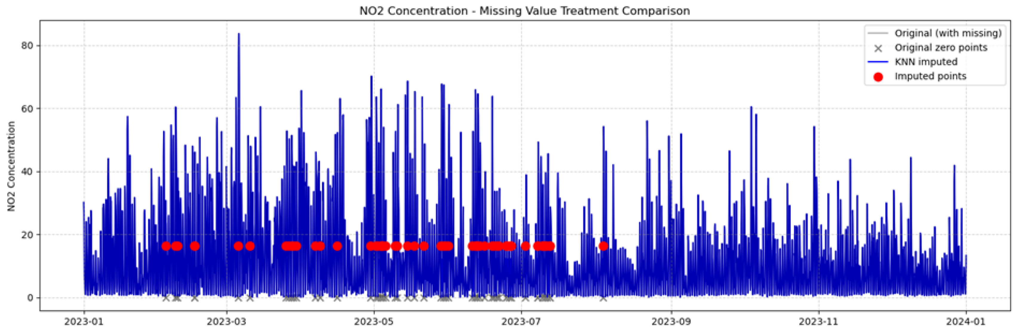
2.1. KNN Interpolation for Missing Values

Before conducting data analysis, this article cleans and preprocesses the raw data to ensure its quality and reliability. The first step is to handle missing values. Due to the strong correlation between air quality data and time, the concentration of pollutants fluctuate dramatically at different time. Traditional mean imputation methods (such as filling missing values with global means) cannot effectively capture the temporal characteristics of the data. Consequently the KNN interpolation methods is most suitable for simulating missing data using surrounding data.

KNN interpolation (K-Nearest Neighbors Interpolation) is a non parametric method based on neighboring samples. The core idea is to calculate the distance between the interpolation point and the known data point, find the nearest K neighbors, and use the values of these neighbors for weighted or average estimation. If we have a missing value ${\widehat{X}}_i$ for feature $X_i$ we use the following formula to impute it based on the k nearest neighbors.

$${\widehat{X}}_i={\displaystyle \frac{1}{k}}\sum _{j\in N_k\left(i\right)}{X}_j$$

(1)

where $N_k\left(i\right)$ is the set of the k nearest neighbors to sample($k=5$), $X_j$ is the feature value of the j-th neighbor, k is the number of nearest neighbors, ${\widehat{X}}_i$ is the imputed value based on the values of the neighbors.[7]

Figure 1. Comparison of KNN interpolation effects.

Figure 1. Comparison of KNN interpolation effects.

2.2. Unit Transformation

In the dataset, the concentration of CO is in ppm and the other pollutants are in $\mu$g/m³, If the raw values with different units are directly substituted into the normalization process, the significant difference in magnitudes will cause the model to overly favor the large values of CO, ignoring the key information of PM. This not only affects the prediction accuracy but also undermines the fairness of the AAQI (Air Quality Index) weighting calculation.

The general conversion formula is(Using Brasilia as an example):

$$Concentration(\mu g/m^3)=Concentration\left(ppm\right)\times {\displaystyle \frac{\mathrm{Molecular}\mathrm{Weight}(\mathrm{g}/\mathrm{mol})}{\mathrm{Gas}\mathrm{Constant}(\mathrm{L}·\mathrm{atm}/\mathrm{mol}·\mathrm{K})\times \mathrm{Temperature}\left(\mathrm{K}\right)}}\times {\displaystyle \frac{\mathrm{P}}{{\mathrm{P}}_0}}\times {10}^6$$

Where: P is the atmospheric pressure in Brasília (95 kPa = 0.95 atm), ${\mathrm{P}}_0$ is the standard atmospheric pressure (101.325 kPa = 1 atm), T is the temperature (295 K).

Concentration ($\mu$g/m³) ≈ Concentration (ppm) × 1.148

Therefore, at the atmospheric pressure and temperature in Brasilia, 1 ppm of CO is approximately 1.148 $\mu$g/m³.[8]

2.3. Data Normalization

Data normalization is aiming to eliminate the influence of different index sizes, the min-max normalization method is used to normalize all data to the [0,1] interval. The standardized formula is as follows:

$$X^{\prime }={\displaystyle \frac{X-X_{min}}{X_{max}-X_{min}}}$$

(2)

Where$X^{\prime }$ is the normalized value, $X_{min}$ is the minimum value of features, $X_{max}$ is the maximum value of features, X is the Original eigenvalue.[9]

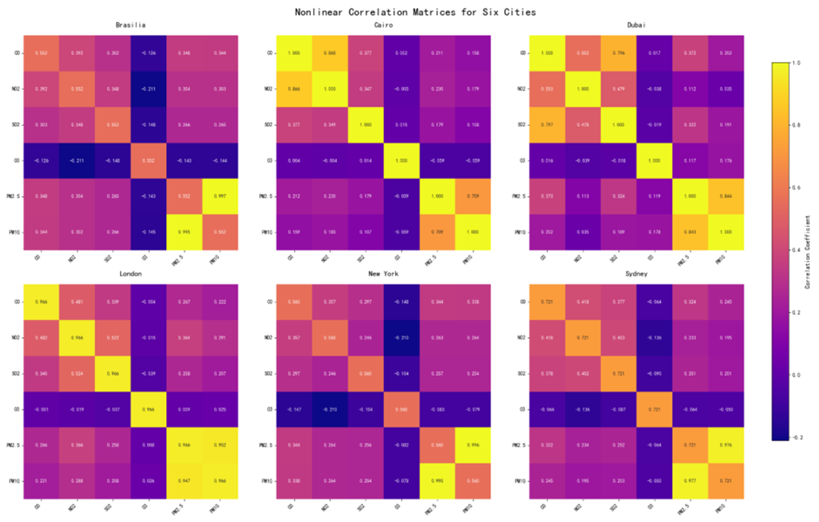
2.4. Calculation of Nonlinear Correlations

After that, researchers want to understand the interactions and impact relationships between various pollutants, so we calculate nonlinear correlations. Because traditional correlations calculation method such as Pearson correlation applies to the linear relationships, three methods are employed to compute the correlation between pollutants in this research, which is beneficial to measure nonlinear relationships.

Mutual Information measures the amount of information shared between two variables, capturing both linear and nonlinear dependencies. MI is particularly useful for identifying relationships that might be overlooked by traditional correlation methods. The MI between pollutants X and Y is computed using the following formula:

$$\mathrm{I}\left(\mathrm{X};\mathrm{Y}\right)=\sum _{\mathrm{x}\in \mathrm{X}}\sum _{\mathrm{y}\in \mathrm{Y}}\mathrm{p}\left(\mathrm{x},\mathrm{y}\right)\log \left({\displaystyle \frac{\mathrm{p}\left(\mathrm{x},\mathrm{y}\right)}{\mathrm{p}\left(\mathrm{x}\right)\mathrm{p}\left(\mathrm{y}\right)}}\right)$$

Where: $\mathrm{p}\left(\mathrm{x},\mathrm{y}\right)$ is the joint probability distribution of the two variables, and $\mathrm{p}\left(\mathrm{x}\right)$ and $\mathrm{p}\left(\mathrm{y}\right)$ are the marginal distributions.[10]

Spearman’s correlation assesses the monotonic relationship between two variables by comparing their ranks rather than their actual values. It is particularly useful for capturing nonlinear, monotonic dependencies. The Spearman correlation coefficient $\rho$ is calculated as:

$$\rho =1-{\displaystyle \frac{6\sum {\mathrm{d}}_{\mathrm{i}}^2}{\mathrm{n}\left({\mathrm{n}}^2-1\right)}}$$

Where: ${\mathrm{d}}_{\mathrm{i}}$ is the difference in ranks for each data pair, and n is the number of data points.[11]

Kendall’s Tau measures the degree of concordance and discordance between pairs of data points. It is also based on ranks, but unlike Spearman’s, it uses a pairwise comparison approach. The Kendall Tau coefficient $\tau$ is computed as:

$$\tau ={\displaystyle \frac{\mathrm{C}-\mathrm{D}}{\frac{\mathrm{n}\left(\mathrm{n}-1\right)}{2}}}$$

where C is the number of concordant pairs and D is the number of discordant pairs. [12]

Combined Correlation Matrix To capture the full range of dependencies between pollutants, a weighted combination of the three correlation methods is used. The final combined correlation matrix ${\mathrm{M}}_{\mathrm{combined}}$ is calculated as:

$${\mathrm{M}}_{\mathrm{combined}}=0.6\times {\mathrm{M}}_{\mathrm{MI}}+0.3\times {\mathrm{M}}_{\mathrm{Spearman}}+0.1\times {\mathrm{M}}_{\mathrm{Kendall}}$$

This combined approach allows for a more nuanced understanding of the interdependencies between pollutants, integrating both linear and nonlinear relationships.

Figure 2. Heat map of air pollutant correlation coefficient from six different cities.

Figure 2. Heat map of air pollutant correlation coefficient from six different cities.

3. Predicting Air Quality by Time-Weighted Ensemble Model

In this section, we take LSTM, DNN, RF and ARIMA models into considerations, which are highly sensitive to time and have shown good results in series predictions before.

3.1. Long Short-Term Memory (LSTM)

The Long Short-Term Memory (LSTM) model is a type of recurrent neural network (RNN) designed to effectively capture long-term dependencies in sequential data. It can automatically learn the optimal temporal lag structure from the data, eliminating the need for manual lag selection and model complex temporal and nonlinear relationships, by incorporating nonlinear activation functions, which is very suitable for predict the air quality.An LSTM cell contains three key gates — the input gate, forget gate, and output gate — which regulate the flow of information. The gating structure allows LSTM to selectively retain or forget information, enhancing robustness when dealing with noisy or irregular input data.The model formulas are as follows:

$${\mathrm{f}}_{\mathrm{t}}=\sigma \left({\mathrm{W}}_{\mathrm{f}}·\left[{\mathrm{h}}_{\mathrm{t}-1},{\mathrm{x}}_{\mathrm{t}}\right]+{\mathrm{b}}_{\mathrm{f}}\right)$$

$${\mathrm{i}}_{\mathrm{t}}=\sigma \left({\mathrm{W}}_{\mathrm{i}}·\left[{\mathrm{h}}_{\mathrm{t}-1},{\mathrm{x}}_{\mathrm{t}}\right]+{\mathrm{b}}_{\mathrm{i}}\right)$$

$${\tilde{C}}_{\mathrm{t}}=\tan \mathrm{h}\left({\mathrm{W}}_{\mathrm{C}}·\left[{\mathrm{h}}_{\mathrm{t}-1},{\mathrm{x}}_{\mathrm{t}}\right]+{\mathrm{b}}_{\mathrm{C}}\right)$$

$${\mathrm{C}}_{\mathrm{t}}={\mathrm{f}}_{\mathrm{t}}\odot {\mathrm{C}}_{\mathrm{t}-1}+{\mathrm{i}}_{\mathrm{t}}\odot {\tilde{C}}_{\mathrm{t}}$$

$${\mathrm{o}}_{\mathrm{t}}=\sigma \left({\mathrm{W}}_{\mathrm{o}}·\left[{\mathrm{h}}_{\mathrm{t}-1},{\mathrm{x}}_{\mathrm{t}}\right]+{\mathrm{b}}_{\mathrm{o}}\right)$$

$${\mathrm{h}}_{\mathrm{t}}={\mathrm{o}}_{\mathrm{t}}\odot \tan \mathrm{h}\left({\mathrm{C}}_{\mathrm{t}}\right)$$

Where, ${\mathrm{x}}_{\mathrm{t}}$ is the input at time step t, ${\mathrm{h}}_{\mathrm{t}}$ is the hidden state, ${\mathrm{C}}_{\mathrm{t}}$ is the cell state, ${\mathrm{f}}_{\mathrm{t}}$, ${\mathrm{i}}_{\mathrm{t}}$, and ${\mathrm{o}}_{\mathrm{t}}$ denote the forget, input, and output gates respectively, $\sigma$ is the sigmoid activation function, and ⊙ represents element-wise multiplication.[13]

3.2. Deep Neural Networks (DNN)

Deep Neural Networks (DNN) is a type of artificial neural network with multiple layers between the input and output layers. DNN is good at capturing complex, non-linear relationships in data. Air quality data often exhibits non-linear trends, seasonal variations, and other complex behaviors. DNNs can model these non-linear relationships without explicitly needing to define them, which can lead to better predictive performance.The model formulas are as follows:

$${\mathrm{a}}^{\left(\mathrm{l}\right)}=\sigma \left({\mathrm{W}}^{\left(\mathrm{l}\right)}·{\mathrm{a}}^{\left(\mathrm{l}-1\right)}+{\mathrm{b}}^{\left(\mathrm{l}\right)}\right)$$

$$\mathrm{MSE}={\displaystyle \frac{1}{\mathrm{n}}}\underset{\mathrm{i}=1}{\sum ^{\mathrm{n}}}{\left({\mathrm{y}}_{\mathrm{i}}-{\widehat{y}}_{\mathrm{i}}\right)}^2$$

$${\mathrm{W}}^{\left(\mathrm{l}\right)}={\mathrm{W}}^{\left(\mathrm{l}\right)}-\eta ·{\displaystyle \frac{\partial \mathrm{L}}{\partial {\mathrm{W}}^{\left(\mathrm{l}\right)}}}$$

$${\mathrm{b}}^{\left(\mathrm{l}\right)}={\mathrm{b}}^{\left(\mathrm{l}\right)}-\eta ·{\displaystyle \frac{\partial \mathrm{L}}{\partial {\mathrm{b}}^{\left(\mathrm{l}\right)}}}$$

$$\widehat{y}={\mathrm{W}}^{\left(\mathrm{L}\right)}·{\mathrm{a}}^{\left(\mathrm{L}-1\right)}+{\mathrm{b}}^{\left(\mathrm{L}\right)}$$

Where, ${\mathrm{W}}^{\left(\mathrm{l}\right)}$ is the weight matrix for layer l, ${\mathrm{a}}^{\left(\mathrm{l}-1\right)}$ is the output of the previous layer (for the first layer, it is the input X), ${\mathrm{b}}^{\left(\mathrm{l}\right)}$ is the bias vector for layer l, $\sigma$ is the activation function ($\sigma \left(\mathrm{x}\right)=\max \left(0,\mathrm{x}\right)$ (ReLU) for hidden layers, linear for the output layer), ${\mathrm{a}}^{\left(\mathrm{l}\right)}$ is the output (activation) of layer l, ${\mathrm{y}}_{\mathrm{i}}$ is the true value (target), ${\widehat{y}}_{\mathrm{i}}$ is the predicted value from the model, n is the number of data points, $\eta$ is the learning rate, ${\displaystyle \frac{\partial \mathrm{L}}{\partial {\mathrm{W}}^{\left(\mathrm{l}\right)}}}$ and ${\displaystyle \frac{\partial \mathrm{L}}{\partial {\mathrm{b}}^{\left(\mathrm{l}\right)}}}$ are the gradients of the loss function with respect to the weights and biases, respectively, L is the final (output) layer of the network, ${\mathrm{a}}^{\left(\mathrm{L}-1\right)}$ is the output of the last hidden layer, ${\mathrm{W}}^{\left(\mathrm{L}\right)}$ and ${\mathrm{b}}^{\left(\mathrm{L}\right)}$ are the weight matrix and bias vector of the output layer.[14]

3.3. Random Forest (RF)

Random Forest is an ensemble learning method based on multiple decision trees, which can capture complex non-linear relationships and interactions between features. It is less sensitive to overfitting and works well with noisy data, making it reliable for real-world air quality predictions where noise and outliers are common. The random forest regression formula is:

$${\widehat{y}}_{\mathrm{i}}={\mathrm{f}}_{\mathrm{i}}\left(\mathrm{X}\right)$$

$$\widehat{y}={\displaystyle \frac{1}{\mathrm{N}}}\underset{\mathrm{i}=1}{\sum ^{\mathrm{N}}}{\widehat{y}}_{\mathrm{i}}$$

Where, ${\widehat{y}}_{\mathrm{i}}$ is the prediction from the i-th decision tree, X is the input feature vector, ${\mathrm{f}}_{\mathrm{i}}$ is the function learned by the i-th decision tree, which outputs a predicted value based on, $\widehat{y}$ is the final prediction, N is the number of trees in the forest.[15]

3.4. Autoregressive Integrated Moving Average (ARIMA)

Autoregressive Integrated Moving Average Model(ARIMA) is a statistical model used for time series prediction. By combining autoregression (AR), differencing (I), and moving average (MA), ARIMA is able to capture trends and seasonal variations in data. The preponderance of ARIMA is strong adaptability, which can handle various time series data like . The general ARIMA(p, d, q) model can be written as:

$${\mathrm{y}}_{\mathrm{t}}=\mathrm{c}+\underset{\mathrm{i}=1}{\sum ^{\mathrm{p}}}{\varphi }_{\mathrm{i}}{\mathrm{y}}_{\mathrm{t}-\mathrm{i}}+\underset{\mathrm{j}=1}{\sum ^{\mathrm{q}}}{\theta }_{\mathrm{j}}{ϵ}_{\mathrm{t}-\mathrm{j}}+{ϵ}_{\mathrm{t}}$$

Where, ${\mathrm{y}}_{\mathrm{t}}$ is the actual value of the time series at time t, c is a constant (optional, sometimes set to 0), ${\varphi }_{\mathrm{i}}$ are the parameters of the autoregressive part (AR), ${ϵ}_{\mathrm{t}}$ is the error term at time t, also known as the white noise (residuals), ${\theta }_{\mathrm{j}}$ are the parameters of the moving average part (MA), ${ϵ}_{\mathrm{t}-\mathrm{j}}$ are the lagged residuals (errors) from previous time steps, p is the number of lag terms in the autoregressive model, q is the number of lag terms in the moving average model.[16]

The dataset of above four models is divided according to the following method. The training set is from January to October of 2023 (accounting for 83.2%), which is used to learn the seasonal and daily variation patterns of pollutants. Validation set is November of 2023 (accounting for 8.2%), using to optimize hyperparameters of LSTM, DNN, and random forest (such as the number of hidden layer nodes, learning rate, dropout rates, batch size, the number of estimators, max depth and so on ). Test set is December of 2023 (accounting for 8.4%), verifying the generalization ability of the model on recently unknown data.

Because different models have different outcomes, some focus on MAE and some focus on R-squared. In order to improve the accuracy of prediction results, we have created a ensemble model with time weights. We have also invented a new formula for calculating model performance, which adjusts the time weights of each model by maximizing model performance parameters.The performance score combines MAE and R²:

$$\mathrm{Performance}\mathrm{Score}={\displaystyle \frac{1}{1+\mathrm{MAE}}}\times {\displaystyle \frac{{\mathrm{R}}^2+1}{2}}$$

Where, MAE is mean absolute error, which measures accuracy. R² measures goodness of fit.

3.5. Time-Weighted Ensemble Model

The Time-Weighted Ensemble combines the predictions from LSTM, DNN, and Random Forest models based on hourly optimized weights.

Considering that the effect of direct weighting is not much better than a single model, we adopt the hourly weighting method to improve the performance of the ensemble model. The weights for each model are optimized for each hour to minimize the MAE for the ensemble prediction:

$${\widehat{y}}_{\mathrm{ensemble}}=\underset{\mathrm{i}=1}{\sum ^{\mathrm{n}}}{\mathrm{w}}_{\mathrm{i}}·{\widehat{y}}_{\mathrm{i},\mathrm{h}}$$

Where ${\mathrm{w}}_{\mathrm{i}}$ are the weights, and ${\widehat{y}}_{\mathrm{i},\mathrm{h}}$ are the predictions from each model.

In addition, if one model performs significantly better than others (based on the performance ratio), that model is used exclusively for that hour.

4. Predicting Result of Multiple Model

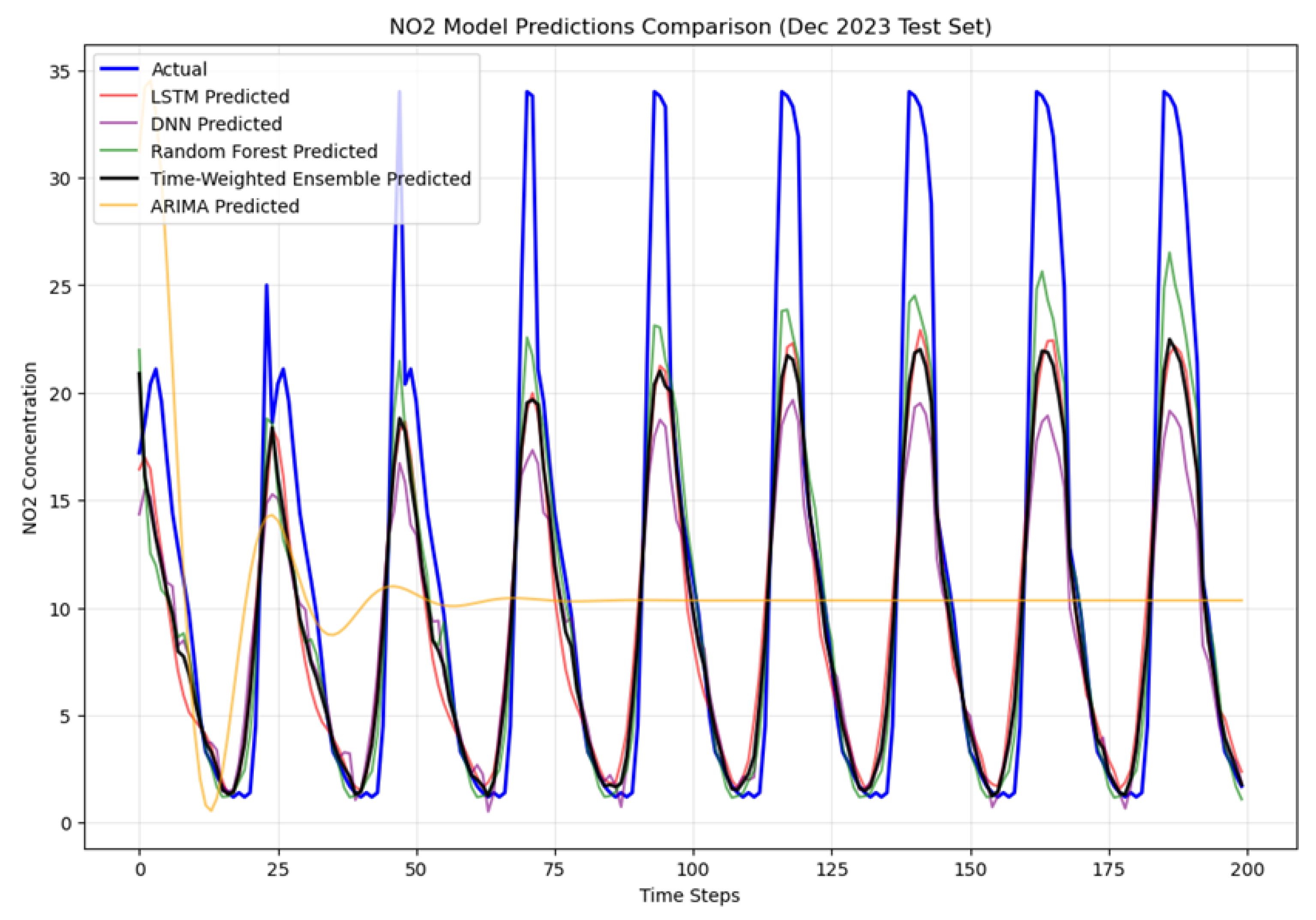
Using Time-Weighted Ensemble model, this study predicted the changes in NO2 concentration throughout 2024 and the NO2 concentration at various times on January 1, 2024, by using the data from December 29, 30 and 31, 2023. The calculated results and actual pollutant concentrations are as follows:

Figure 3. CO concentration throughout 2023.

Figure 3. CO concentration throughout 2023.

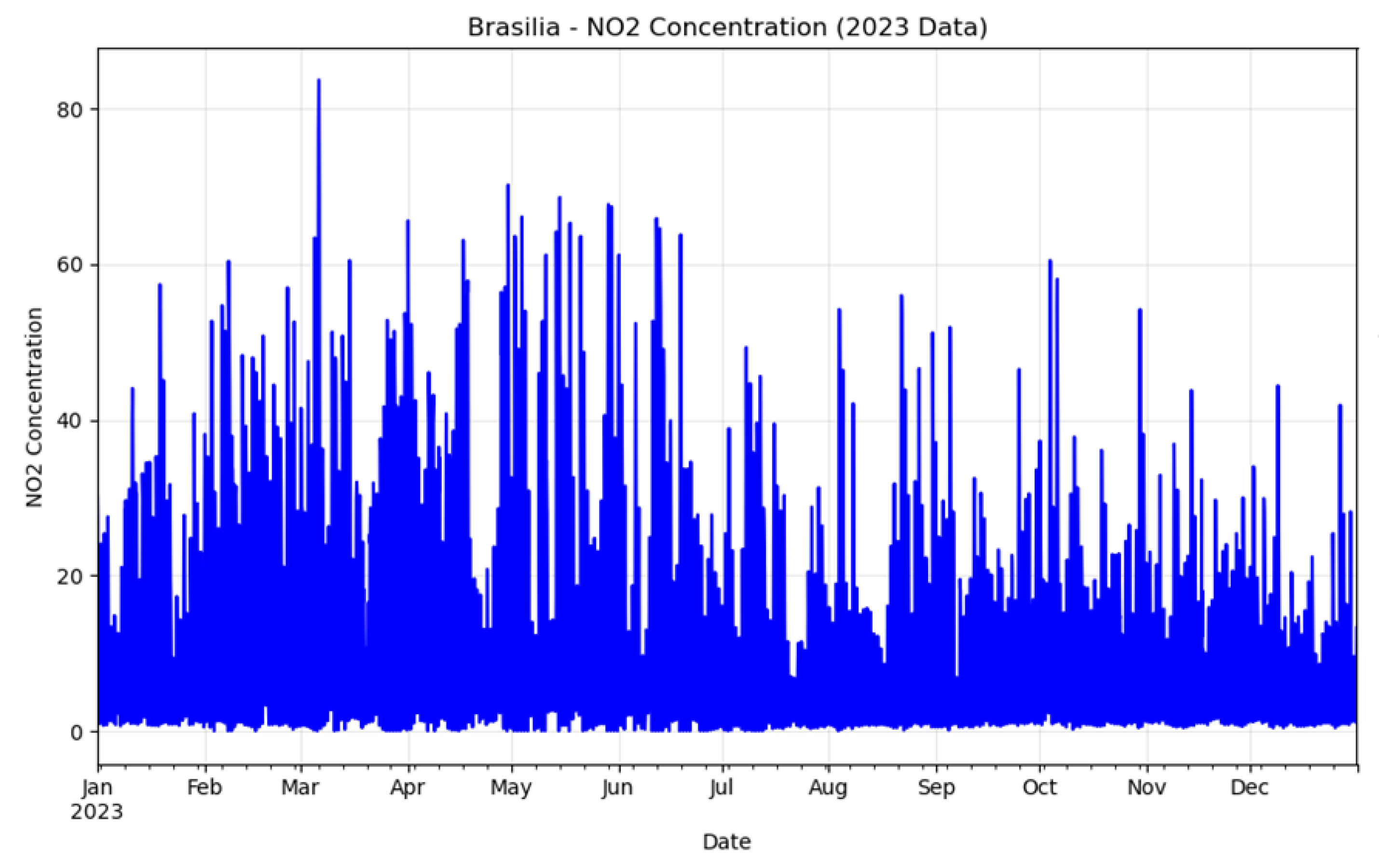
Figure 4. Line chart of CO concentration.

Figure 4. Line chart of CO concentration.

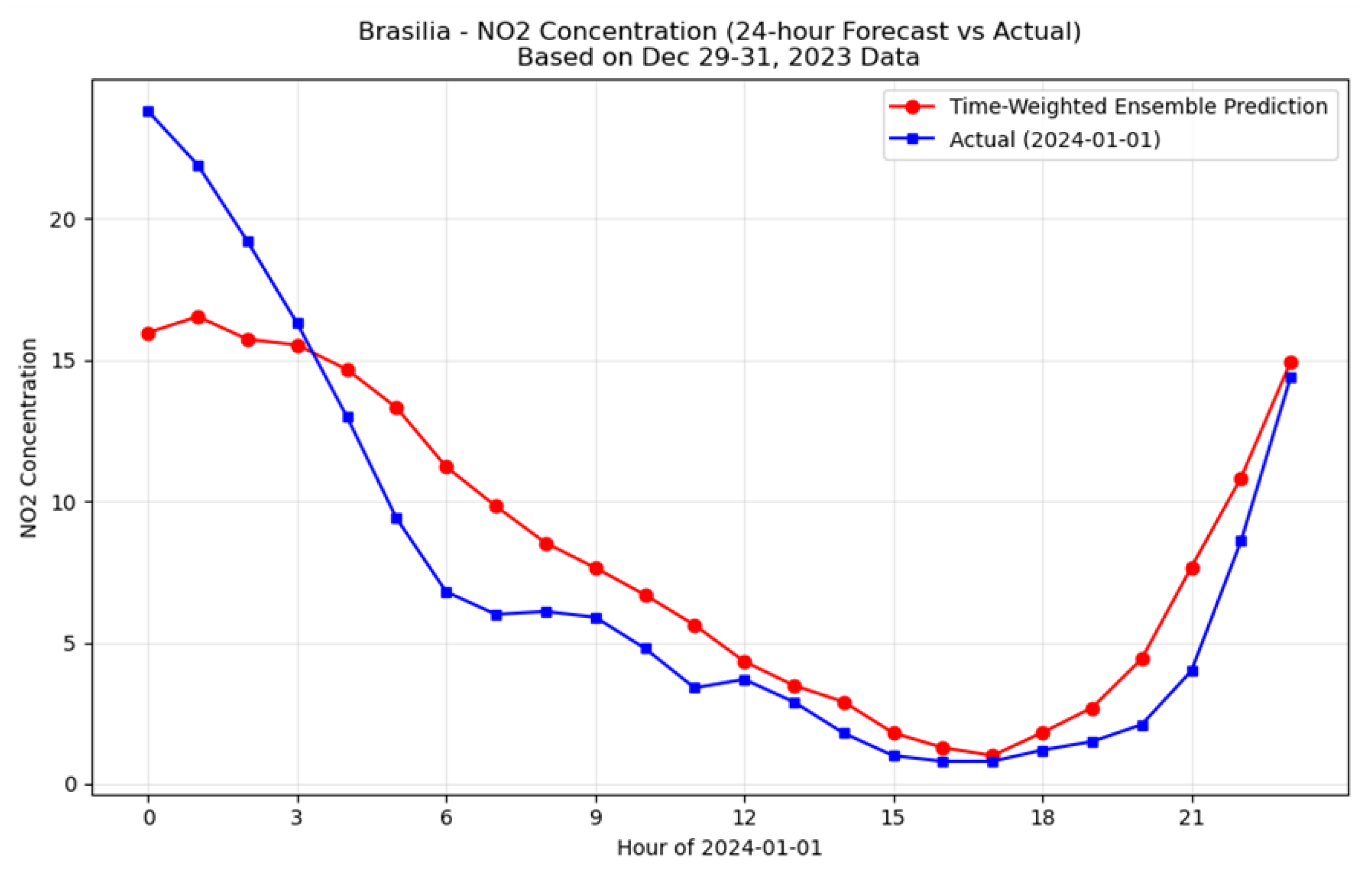
In the predicted results, most of the NO2 concentrations in Brasilia are around 20$\mu \mathrm{g}/{\mathrm{m}}^3$and the maximum concentration is more than 80$\mu \mathrm{g}/{\mathrm{m}}^3$ in March. And the NO2 concentration of 2024.1.1 is decreasing from 15 $\mu \mathrm{g}/{\mathrm{m}}^3$ at 0 o’clock and get the lowest point at around 16 o’clock, then increasing to 14 $\mu \mathrm{g}/{\mathrm{m}}^3$ at the end of the day. Although some values have differences, the two lines decreasing and increasing simultaneously, indicating that the model has good predictive performance. The MAE of this prediction is only 2.25 and the R-squared is up to 0.82.

Afterwards, we draw the comparison graph of 5 models and the actual data. Most of the models can capture the oscillation, the lowest NO2 concentration of forecast result is almost same as the actual data and the highest one is much lower than the acutal data. However, it is easily found that ARIMA has a bad performance in fitting periodicity data, which just captures two oscillation cycles.

Figure 5. NO2 model predictions comparison.

Figure 5. NO2 model predictions comparison.

5. Model Fit Analysis

In order to evaluate the accuracy and precision of the model prediction results, we use the mean absolute error(MAE) and mean absolute percentage error(MAPE) for measurement.

Mean Absolute Error (MAE) is the average absolute difference between predicted and true values, calculated using the following formula:

$$\mathrm{MAE}={\displaystyle \frac{1}{\mathrm{N}}}\underset{\mathrm{i}=1}{\sum ^{\mathrm{N}}}\left|{\mathrm{y}}_{\mathrm{i}}-{\widehat{y}}_{\mathrm{i}}\right|$$

Where, ${\mathrm{y}}_{\mathrm{i}}$ is the actual value, ${\widehat{y}}_{\mathrm{i}}$ is the predicted value, N is the number of sample.[17]

The R-squared (R²), also known as the coefficient of determination, is a statistical measure that represents the proportion of the variance in the dependent variable that is explained by the independent variables in a regression model. Formula for R-squared (R²):

$${\mathrm{R}}^2=1-{\displaystyle \frac{{\sum }_{\mathrm{i}=1}^{\mathrm{n}}{\left({\mathrm{y}}_{\mathrm{i}}-{\widehat{y}}_{\mathrm{i}}\right)}^2}{{\sum }_{\mathrm{i}=1}^{\mathrm{n}}{\left({\mathrm{y}}_{\mathrm{i}}-\mathrm{y}\right)}^2}}$$

Where, ${\mathrm{y}}_{\mathrm{i}}$ is the actual value of the dependent variable for the i-th observation, ${\widehat{y}}_{\mathrm{i}}$ is the predicted value of the dependent variable for the i-th observation, y is the mean of the actual values of the dependent variable, n is the number of observations.[18]

The following two images show the difference between the predicted value and the true value and the distribution of the prediction error.

Figure 6. MAE comparison of five models.

Figure 6. MAE comparison of five models.

Figure 7. R² comparison of five models.

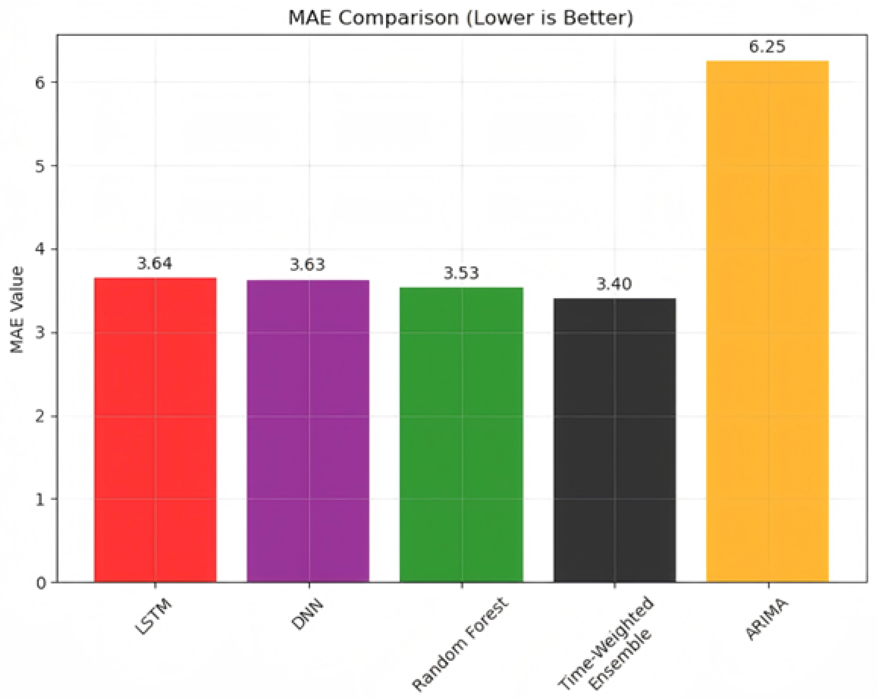
Figure 7. R² comparison of five models.

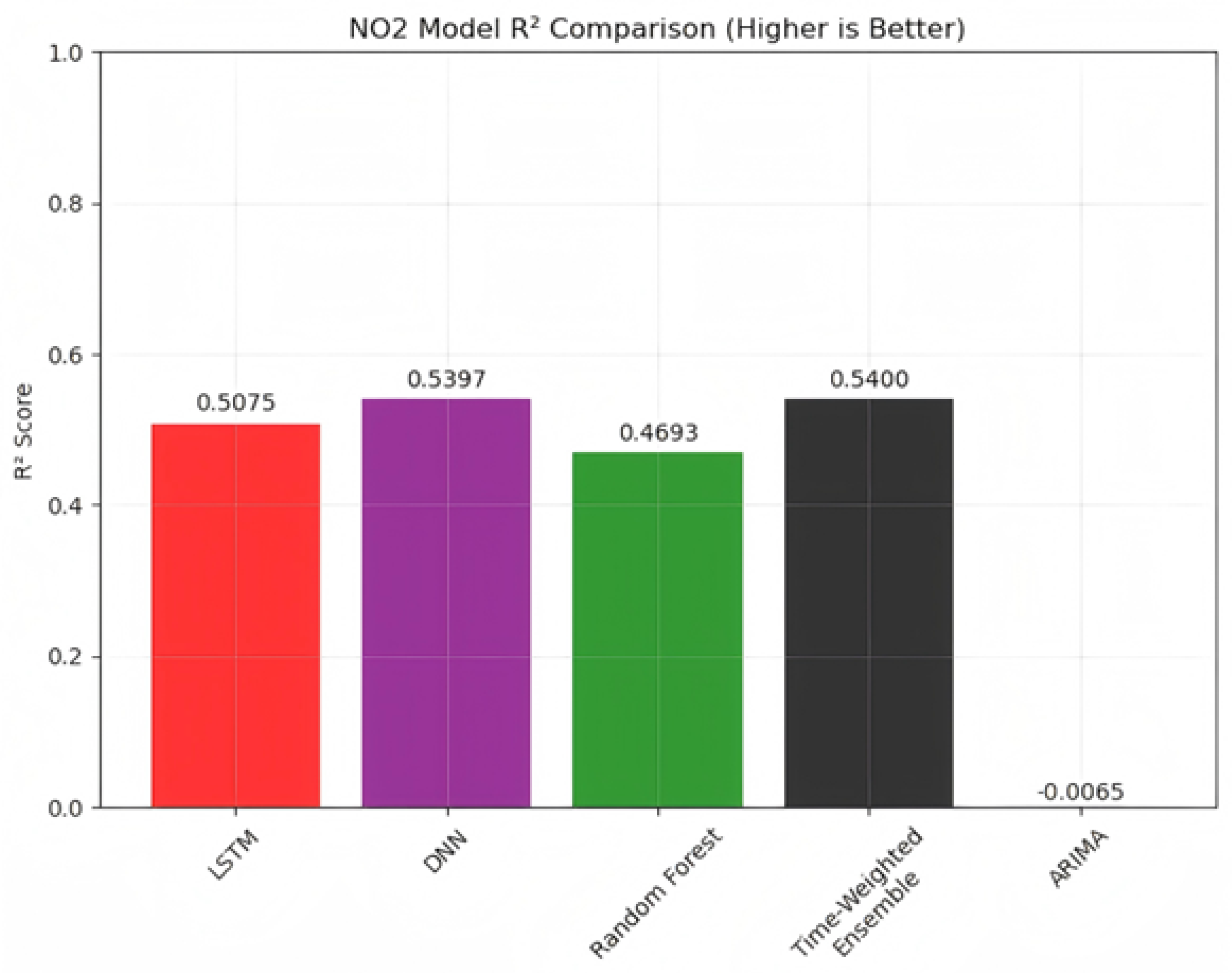
Figure 8. Prediction error distribution.

Figure 8. Prediction error distribution.

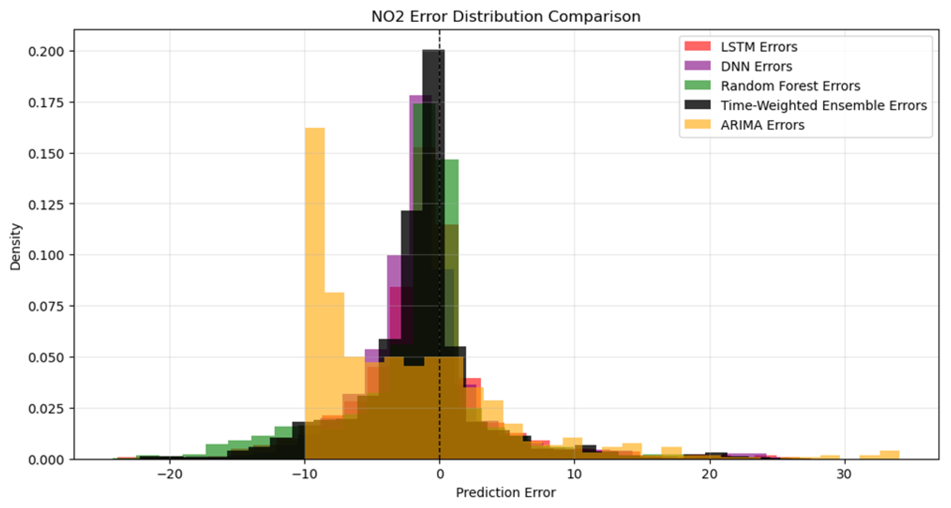
According to the figure, the MAE of Time-Weighted ensemble model is smaller than other 4 model and the ensemble model also has the best performance in R². Most of the error distribution present a normal distribution, but the ARIMA error distribution get highest density around -10, this is because it did not capture the periodic pattern and get a stable prediction result.

Although, air quality prediction is inherently challenging due to the highly dynamic, nonlinear, and multiscale nature of the atmospheric system, The MAE only 3.40 and the R² is 0.54 showing that Time-Weighted ensemble model predicting model still has a good performance in prediction and the error is relatively small.

Figure 9. model performance comparison.

Figure 9. model performance comparison.

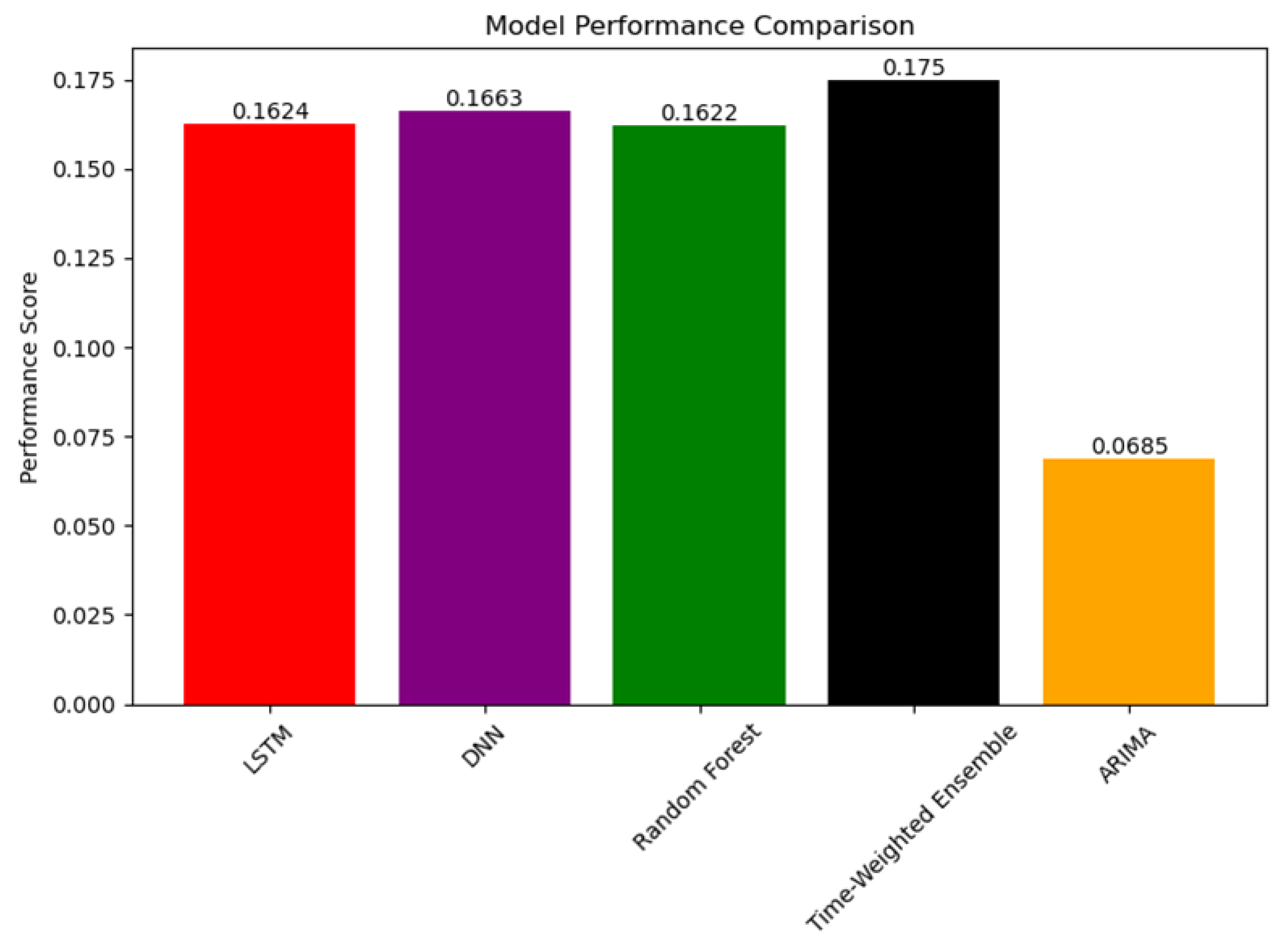
We calculated the model performance score by using the performance score function, Time-Weighted ensemble function get the highest score, which improves by 5.23% compared to a single best model.

In addition, we also recorded the model training process and print the training loss function and validation loss function of two neural network model, which are important components of ensemble model.

Figure 10. training loss and validation loss of LSTM and DNN.

Figure 10. training loss and validation loss of LSTM and DNN.

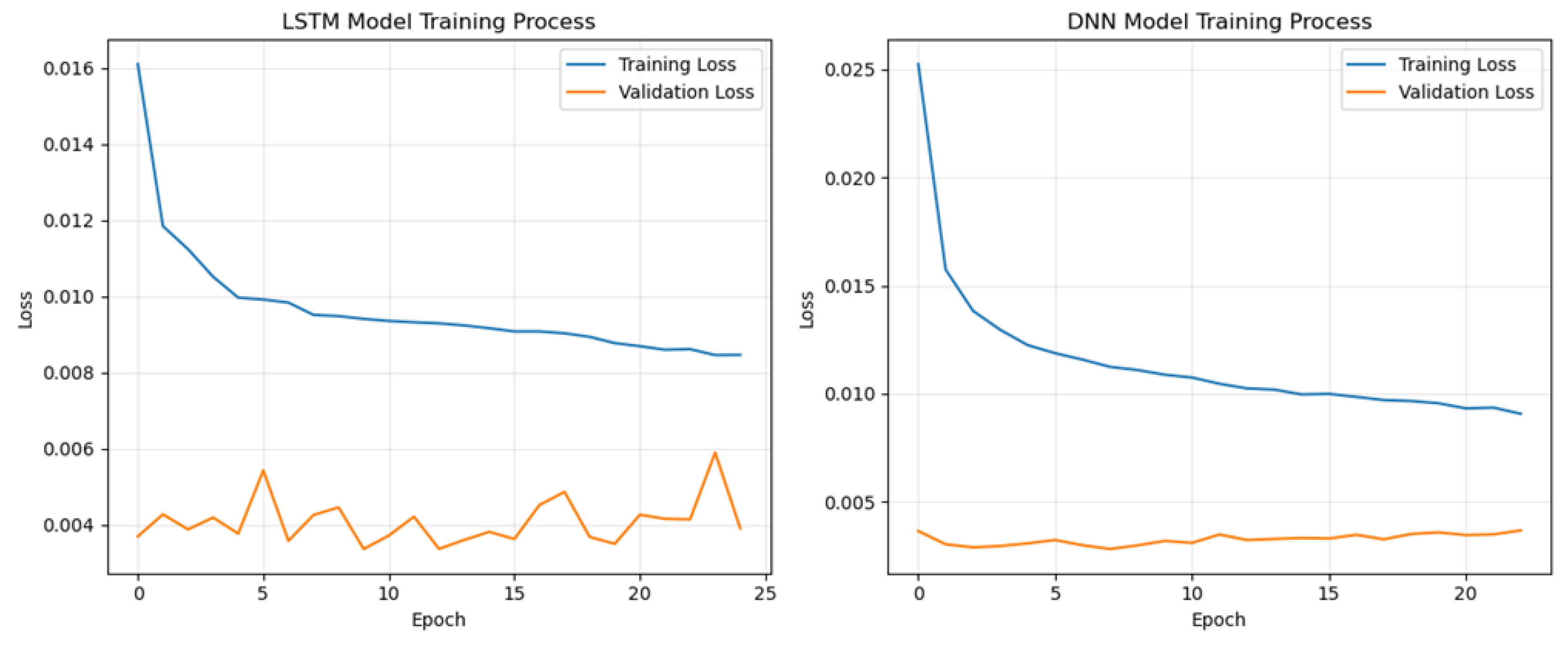
The training loss of LSTM continuously decreases from around 0.016 to approximately 0.009, indicating that the model is effectively learning and fitting the training data, showing a clear convergence trend. The validation loss remains relatively low and stable, within the range of about 0.004 to 0.005, suggesting that the model maintains a small error on the validation set and demonstrates good generalization ability. And the training loss of DNN also decreases dramatically, from 0.025 to 0.009,the validation loss is always less than 0.005.

6. Establishment of Adaptive Air Quality Model

Adaptive air quality model formula:

For every pollutants $\mathrm{p}\in \mathrm{P}$, where $\mathrm{P}=\left\{\mathrm{P}{\mathrm{M}}_{2.5},\mathrm{P}{\mathrm{M}}_{10},{\mathrm{O}}_3,\mathrm{N}{\mathrm{O}}_2,\mathrm{CO},\mathrm{S}{\mathrm{O}}_2\right\}$, considering that the impact of pollutants on human health is non-linear, we assign an influence coefficient and a safety threshold to each pollutant. After exceeding the safety threshold, ${\mathrm{I}}_{\mathrm{p}}$ will exponentially increase. The health impact values of pollutants ${\mathrm{I}}_{\mathrm{p}}$ is defined as:

$${\mathrm{I}}_{\mathrm{p}}=\left\{\begin{array}{cc}{\mathrm{B}}_{\mathrm{p}}\left[{\left({\displaystyle \frac{{\mathrm{C}}_{\mathrm{p}}}{{\mathrm{T}}_{\mathrm{p}}}}\right)}^{{\mathrm{E}}_{\mathrm{p}}}-1\right]\hfill & \mathrm{if}{\mathrm{C}}_{\mathrm{p}}>{\mathrm{T}}_{\mathrm{p}}\\ 0\hfill & \mathrm{otherwise}\end{array}\right.$$

Where, ${\mathrm{C}}_{\mathrm{p}}$ is pollutant concentration, ${\mathrm{T}}_{\mathrm{p}}$ is safety threshold, ${\mathrm{B}}_{\mathrm{p}}$ is basic influence coefficient, ${\mathrm{E}}_{\mathrm{p}}$ is nonlinear index[19]

Table 1. Numerical value of ${\mathrm{T}}_{\mathrm{p}}$, ${\mathrm{B}}_{\mathrm{p}}$ and ${\mathrm{E}}_{\mathrm{p}}$ .

p	${\mathbf{T}}_{\mathbf{p}}$($\mathit{\mu }\mathbf{g}/{\mathbf{m}}^3$)[20]	${\mathbf{B}}_{\mathbf{p}}$[21,22]	${\mathbf{E}}_{\mathbf{p}}$
PM2.5	15	0.35	1.8
PM10	45	0.25	1.6
O3	50	0.30	2.0
NO2	20	0.20	1.7
CO	230	0.15	1.5
SO2	40	0.10	1.9

Table 1. Numerical value of ${\mathrm{T}}_{\mathrm{p}}$, ${\mathrm{B}}_{\mathrm{p}}$ and ${\mathrm{E}}_{\mathrm{p}}$ .

p	${\mathbf{T}}_{\mathbf{p}}$($\mathit{\mu }\mathbf{g}/{\mathbf{m}}^3$)[20]	${\mathbf{B}}_{\mathbf{p}}$[21,22]	${\mathbf{E}}_{\mathbf{p}}$
PM2.5	15	0.35	1.8
PM10	45	0.25	1.6
O3	50	0.30	2.0
NO2	20	0.20	1.7
CO	230	0.15	1.5
SO2	40	0.10	1.9

Considering the synergistic or antagonistic effects between pollutants, we have designed correlation of pollutants adjustment weight which allocates the weights scientifically:

$${{\mathrm{W}}_{\mathrm{p}}}^{\prime }={\mathrm{W}}_{\mathrm{p}}·\left(1+{\mathrm{r}}_{\mathrm{p}}\right)$$

$$r_p={\displaystyle \frac{1}{N-1}}\sum _{q\ne p}{C}_{pq}$$

where, ${\mathrm{W}}_{\mathrm{p}}$ is original weight, ${\mathrm{r}}_{\mathrm{p}}$ is average correlation coefficient, N is the number of air pollution, $C_{pq}$ is the correlation coefficient between pollutant p and q in the comprehensive correlation coefficient matrix. ${{\mathrm{W}}_{\mathrm{p}}}^{\prime }$ is adjust weight.

Adjusted AAQI value is the weighted sum of all pollutant health impact values:

$$\mathrm{AAQI}=\sum _{\mathrm{p}\in \mathrm{P}}{\mathrm{I}}_{\mathrm{p}}·{{\mathrm{W}}^{\prime }}_{\mathrm{p}}$$

Due to the fact that most people are commuting between 7-9 in the morning and 5-7 in the afternoon, and are exposed to more outdoor air pollutants, the impact of air quality on human health is greatest during this period. 10a.m.-16p.m. and 20p.m.-22p.m. are relatively active but generally indoors, while the rest of the time is late at night, mainly during sleep time. They breathe less air and are indoors, so the impact of air quality on human health is minimal during this period. Therefore the time weight factor is defined as:

$${\mathrm{W}}_{\mathrm{t}}=\left\{\begin{array}{cc}1.4\hfill & \mathrm{if}\mathrm{h}\in \left[7,9\right]\mathrm{and}\left[17,19\right]\\ 1.2\hfill & \mathrm{if}\mathrm{h}\in \left[10,16\right]\\ 1.1\hfill & \mathrm{if}\mathrm{h}\in \left[20,22\right]\\ 1.0\hfill & \mathrm{else}\end{array}\right.$$

Where, t represents hour (24 hours per day).

When multiple pollutants coexist, the hazards will be superimposed.[23] We objectively measure the interactions between pollutants using correlation coefficients. The synergistic coefficient is defined as:

$$\mathrm{S}=\left\{\begin{array}{cc}1+0.5·\left|{\displaystyle \frac{1}{\mathrm{N}}}\underset{\mathrm{i}=1}{\sum ^{\mathrm{k}}}\underset{\mathrm{j}=\mathrm{i}+1}{\sum ^{\mathrm{k}}}{\mathrm{r}}_{{\mathrm{p}}_{\mathrm{i}}{\mathrm{p}}_{\mathrm{j}}}\right|\hfill & \mathrm{k}\ge 2\\ 1\hfill & \mathrm{k}<2\end{array}\right.$$

Where, k is the quantity of pollutants exceeding the standard (${\mathrm{C}}_{\mathrm{p}}>{\mathrm{T}}_{\mathrm{p}}$), ${\mathrm{r}}_{{\mathrm{p}}_{\mathrm{i}}{\mathrm{p}}_{\mathrm{j}}}$: correlation coefficient between ${\mathrm{p}}_{\mathrm{i}}$ and ${\mathrm{p}}_{\mathrm{j}}$ , $\mathrm{N}=\left(\begin{array}{c}\mathrm{k}\\ 2\end{array}\right)={\displaystyle \frac{\mathrm{k}\left(\mathrm{k}-1\right)}{2}}$ is the number of combinations of excessive pollutants.

The difference between the correlation coefficient here and the previous one is that S can be flexibly adjusted according to the different correlation coefficients of pollutants in each city, while the previous only focused on the degree of impact of individual pollutants on health.

The final air quality index is:

$$\mathrm{AAQ}{\mathrm{I}}_{\mathrm{final}}=\mathrm{AAQI}·{\mathrm{W}}_{\mathrm{t}}·\mathrm{S}$$

Classification of Air Quality Levels:

Table 2. AAQI range and corresponding level and health proposal .

AAQI range	Level	Health Proposal
[0, 15]	Excellent	Recommed engaging in outdoor acctivities
(15, 30]	Good	Suitable for outdoor activities
(30, 50]	Lightly Polluted	Vulnerable individuals reduce prolonged outdoor activities
(50, 75]	Moderately Polluted	Reduce prolonged outdoor activities
(75, 100]	Heavily Polluted	Avoid outdoor activities
> 100	Hazardous	Stay indoors and use air purifiers

Table 2. AAQI range and corresponding level and health proposal .

AAQI range	Level	Health Proposal
[0, 15]	Excellent	Recommed engaging in outdoor acctivities
(15, 30]	Good	Suitable for outdoor activities
(30, 50]	Lightly Polluted	Vulnerable individuals reduce prolonged outdoor activities
(50, 75]	Moderately Polluted	Reduce prolonged outdoor activities
(75, 100]	Heavily Polluted	Avoid outdoor activities
> 100	Hazardous	Stay indoors and use air purifiers

7. Research Result

By calculating the above AAQI model, the AAQI indicators of Brasilia for the whole year of 2023, are shown in the following figure:

Figure 11. Brasilia 2023 AAQI map.

Figure 11. Brasilia 2023 AAQI map.

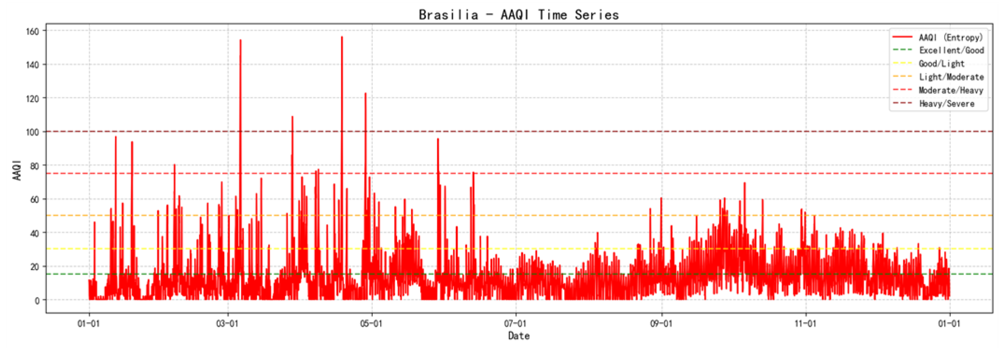
The average AAQI in Brasilia throughout 2023 is 14.11. Furthermore, The biggest numerical value of AAQI in Brasilia is 160 approximately, few of them are more than 30 and most of them are under 15, which shows that Brasilia has excellent air quality and suitable for people to living.

Afterwards, we calculated the average Brasilia 2023 Annual Average Hourly AAQI Index.

Figure 12. Brasilia 2023 Annual Average Hourly AAQI Index.

Figure 12. Brasilia 2023 Annual Average Hourly AAQI Index.

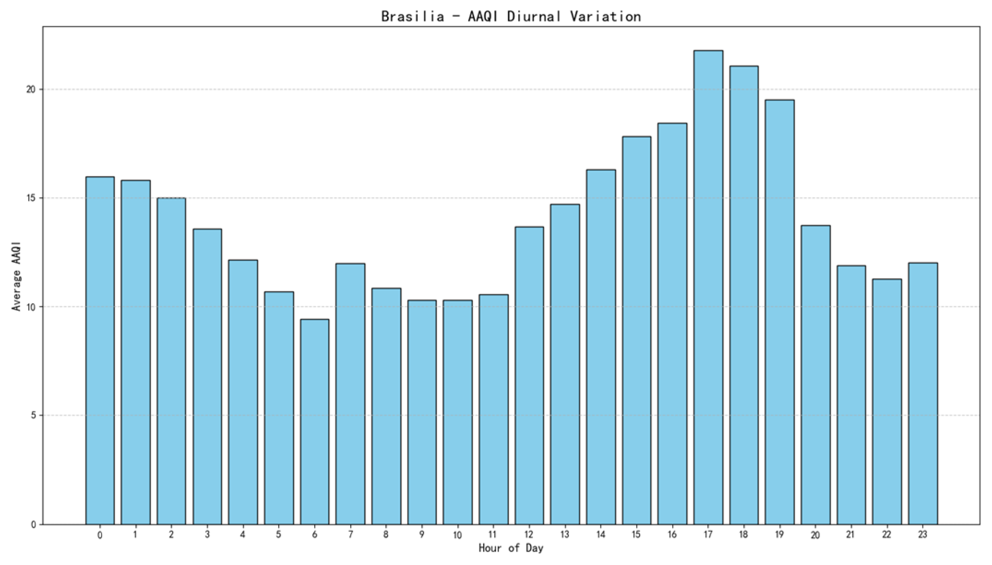
This bar chart shows that Brasilia has good air quality around 5 a.m. to 11a.m., and then AAQI gradually increases, reaching its peak at 17 p.m. After that, AAQI rapidly decreases. It presents the air quality tendency daily.

This study also calculated the proportion of air quality levels in six cities, namely Brasilia, Cairo, Dubai, London, New York, and Sydney, for the whole year of 2023. The results showed that among these six cities, Sydney had the best air quality, with 72.8% of the days having excellent air quality throughout the year, followed by London, Brasilia, New York, and Cairo. Dubai had the worst air quality, with only 0.1% of the days having excellent air quality throughout the year. It also reminded the governors of Dubai and Cairo should pay more attention to the air pollution control.

Figure 13. Proportion of Air Quality Levels in Six Cities in 2023.

Figure 13. Proportion of Air Quality Levels in Six Cities in 2023.

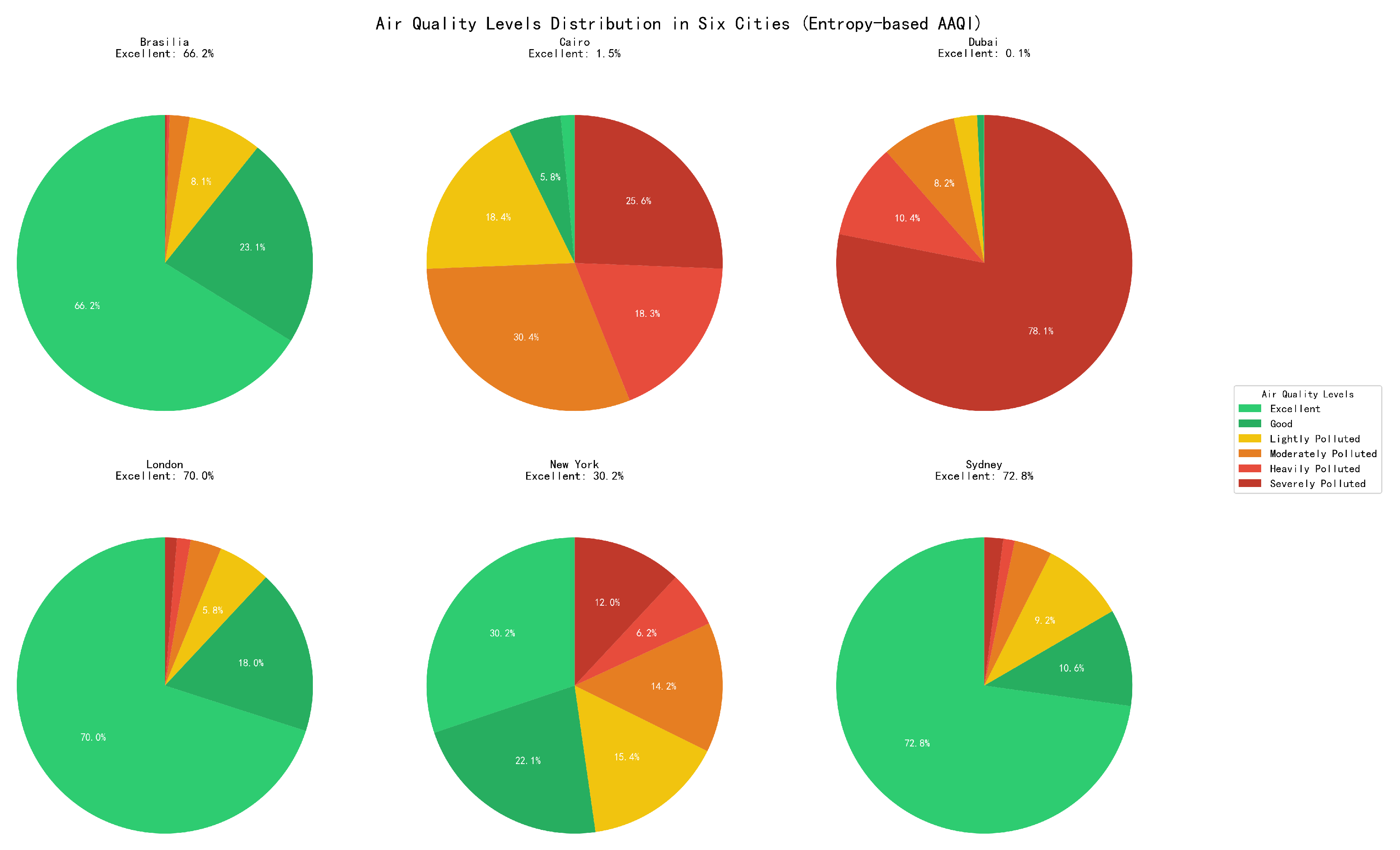
Among them, the deep green air quality level is excellent, the light green air quality level is good, the yellow air quality level is mild pollution, the orange air quality level is moderate pollution, the red air quality level is severe pollution, and the deep red air quality level is dangerous.

8. Conclusion

This study introduced Time-Weighted ensemble model into the air quality prediction model and achieved good results. The prediction results were consistent with reality, and the R-square of prediction is 0.54, which has 5.23% improvement compared to a single best model. Daily forecast result has a better performance, the mean absolute error is 2.25 and the R-squared is up to 0.82. These results offer a practical tool for issuing timely warnings and helping people reduce exposure to air pollution without many data, and the model can be further improved by adding more data sources or extending to multi-site forecasting. It also created the Adaptive Air Quality Index (AAQI), an advanced model that evaluates air quality from four critical dimensions: concentration, correlation, time, and cooperation. By integrating these factors, the AAQI provides a more comprehensive and dynamic assessment than traditional air quality indices. The model not only considers pollutant levels but also the interactions and temporal variations that influence air quality over time. Beyond being an evaluation system, the AAQI serves as an intelligent link between environmental science and public health. Its innovative framework will help establish future air quality management standards, facilitating a shift from reactive monitoring to proactive prevention in environmental health strategies, ensuring more effective and anticipatory protection of public health.

References

- warns severe air pollutions, W. World health organization. Air Quality Guidelines for Europe 2022. [Google Scholar]
- (outdoor) air pollution, A. World health organization. In World Health Organization; 2024. [Google Scholar]
- Li, X.; Peng, L.; Hu, Y. A hybrid model for short-term air quality index forecasting based on mode decomposition and deep learning. Atmospheric Environment 2021, 246, 118096. [Google Scholar]
- Priti, K.; Kumar, P. A critical evaluation of air quality index models (1960–2021). Environmental Monitoring and Assessment 2022, 194. [Google Scholar] [CrossRef] [PubMed]
- Kaggle. Youssef Elebiary. Global Air Quality (2023) - 6 Cities[Data set]. 2024.
- Kaggle. Youssef Elebiary. Global Air Quality (2024) - 6 Cities[Data set]. 2025.
- Taunk, K.; De, S.; Verma, S.; Swetapadma, A. A brief review of nearest neighbor algorithm for learning and classification. 2019 Int Conf Intell Comput Control Syst ICCS 2019, 2019(no. May 2019). [Google Scholar]
- Seinfeld, J.H.; Pandis, S.N. Atmospheric chemistry and physics: from air pollution to climate change; John Wiley & Sons, 2016. [Google Scholar]
- Pedregosa Fabianpedregosa, F.; Michel, V.; Grisel Oliviergrisel, O.; Blondel, M.; Prettenhofer, P.; Weiss, R.; Vanderplas, J.; Cournapeau, D.; Pedregosa, F.; Varoquaux, G.; et al. Scikit-learn: machine learning in Python. [CrossRef]
- Shannon, C.E. A mathematical theory of communication. The Bell system technical journal 1948, 27, 379–423. [Google Scholar] [CrossRef]
- Spearman, C. The proof and measurement of association between two things; 1961. [Google Scholar]
- Kendall, M.G. A new measure of rank correlation. Biometrika 1938, 30, 81–93. [Google Scholar] [CrossRef]
- Hochreiter, S.; Schmidhuber, J. Long short-term memory. Neural computation 1997, 9, 1735–1780. [Google Scholar] [CrossRef] [PubMed]
- LeCun, Y.; Bengio, Y.; Hinton, G. Deep learning. nature 2015, 521, 436–444. [Google Scholar] [CrossRef] [PubMed]
- Breiman, L. Random forests. Machine learning 2001, 45, 5–32. [Google Scholar] [CrossRef]
- Box, G. Box and Jenkins: time series analysis, forecasting and control. In A Very British Affair: Six Britons and the Development of Time Series Analysis During the 20th Century; Springer, 2013; pp. 161–215. [Google Scholar]
- Draper, N.R.; Smith, H. Applied regression analysis; John Wiley & Sons, 1998; Vol. 326. [Google Scholar]
- Neter, J.; Kutner, M.H.; Nachtsheim, C.J.; Wasserman, W.; et al. Applied linear statistical models. 1996. [Google Scholar]
- Miller, N.H.; Molitor, D.; Zou, E. The nonlinear effects of air pollution on health: Evidence from wildfire smoke. Technical report, National Bureau of Economic Research. 2024. [Google Scholar]
- World Health Organization (WHO). Air quality guidelines: Global update 2021. 2021. Available online: https://www.who.int/publications/i/item/9789240034228. [CrossRef]
- Huang, S.; Li, H.; Wang, M.; Qian, Y.; Steenland, K.; Caudle, W.; Liu, Y.; Sarnat, J.; Papatheodorou, S.; ShI, L. Health impacts of long-term exposure to ambient air pollution: A global systematic review and meta-analysis. Science of the Total Environment 2021, 776, 145968. [Google Scholar] [CrossRef] [PubMed]
- Pope, C.A., III; Dockery, D.W. Health effects of fine particulate air pollution: lines that connect. Journal of the air & waste management association 2006, 56, 709–742. [Google Scholar]
- Xia, L.; Zhou, S.; Han, L.; Sun, W.; Sun, H. Joint association of air pollutants on cardiometabolic multimorbidity. Scientific Reports 2024, 14, 26987. [Google Scholar] [CrossRef] [PubMed]
Disclaimer/Publisher’s Note: The statements, opinions and data contained in all publications are solely those of the individual author(s) and contributor(s) and not of MDPI and/or the editor(s). MDPI and/or the editor(s) disclaim responsibility for any injury to people or property resulting from any ideas, methods, instructions or products referred to in the content. |
© 2026 by the authors. Licensee MDPI, Basel, Switzerland. This article is an open access article distributed under the terms and conditions of the Creative Commons Attribution (CC BY) license (http://creativecommons.org/licenses/by/4.0/).
Copyright: This open access article is published under a Creative Commons CC BY 4.0 license, which permit the free download, distribution, and reuse, provided that the author and preprint are cited in any reuse.